Modern Machine Learning for LHC Physicists

Abstract

Modern machine learning is transforming particle physics, faster than we can follow, and bullying its way into our numerical tool box. For young researchers it is crucial to stay on top of this development, which means applying cutting-edge methods and tools to the full range of LHC physics problems. These lecture notes are meant to lead students with basic knowledge of particle physics and significant enthusiasm for machine learning to relevant applications as fast as possible. They start with an LHC-specific motivation and a non-standard introduction to neural networks and then cover classification, unsupervised classification, generative networks, and inverse problems. Two themes defining much of the discussion are well-defined loss functions reflecting the problem at hand and uncertainty-aware networks. As part of the applications, the notes include some aspects of theoretical LHC physics. All examples are chosen from particle physics publications of the last few years. Given that these notes will be outdated already at the time of submission, the week of ML4Jets 2022, they will be updated frequently.

Welcome

These lecture notes are based on lectures in the 2022 Summer term, held at Heidelberg University. These lectures were held on the black board, corresponding to the formula-heavy style, but supplemented with tutorials. The notes start with a very brief motivation why LHC physicists should be interested in modern machine learning. Many people are pointing out that the LHC Run 3 and especially the HL-LHC are going to be a new experiment rather than a continuation of the earlier LHC runs. One reason for this is the vastly increased amount of data and the opportunities for analysis and inference, inspired and triggered by data science as a new common language of particle experiment and theory.

The introduction to neural networks is meant for future particle physicists, who know basic numerical methods like fits or Monte Carlo simulations. All through the notes, we attempt to tell a story through a series of original publications. We start with supervised classification, which is how everyone in particle physics is coming into contact with modern neural networks. We then move on to non-supervised classification, since no ML-application at the LHC is properly supervised, and the big goal of the LHC is to find physics that we do not yet know about. A major part of the lecture notes is then devoted to generative networks, because one of the defining aspects of LHC physics is the combination of first-principle simulations and high-statistics datasets. Finally, we present some ideas how LHC inference can benefit from ML-approaches to inverse problems, a field of machine learning which is less well explored. The last chapter on symbolic regression is meant to remind us that numerical methods are driving much of physics research, but that the language of physics remains formulas, not computer code.

As the majority of authors are German, we would like to add two apologies before we start. First, many of the papers presented in the different sections come from the Heidelberg group. This does not mean that we consider them more important than other papers, but for them we know what we are talking about, and the corresponding tutorials are based on the actual codes used in our papers. Second, we apologize that these lecture notes do not provide a comprehensive list of references beyond the papers presented in the individual chapters. Aside from copyright issues, the idea of these references that it should be easy so switch from a lecture-note mode to a paper-reading mode. For a comprehensive list of references we recommend the Living Review of Machine Learning for Particle Physics [1].

Obviously, these lecture notes are outdated before they even appear on the arXiv. Our plan is to update them regularly, which will also allow us to remove typos, correct wrong arguments and formulas, and improve discussions. Especially young readers who go through these notes from the front to the back, please mark your questions and criticism in a file and send it to us. We will be grateful to learn where we need to improve these notes.

Talking about — we are already extremely grateful to the people who triggered the machine learning activities in our Heidelberg LHC group: Kyle Cranmer, Gregor Kasieczka, Ullrich Köthe, and Manuel Haußmann. We are also extremely grateful to our machine learning collaborators and inspirations, including David Shih, Ben Nachman, Daniel Whiteson, Michael Krämer, Jesse Thaler, Stefano Forte, Martin Erdmann, Sven Krippendorf, Peter Loch, Aishik Ghosh, Eilam Gross, Tobias Golling, Michael Spannowsky, and many others, Next, we cannot thank the ML4Jets community enough, because without those meetings machine learning at the LHC would be as uninspiring as so many other fields, and nothing the unique science endeavor it now is. Finally, we would like to thank all current and former group members in Heidelberg, including Mathias Backes, Marco Bellagente, Lukas Blecher, Sebastian Bieringer, Johann Brehmer, Thorsten Buss, Sascha Diefenbacher, Luigi Favaro, Theo Heimel, Sander Hummerich, Fabian Keilbach, Nicholas Kiefer, Tobias Krebs, Michel Luchmann, Armand Rousselot, Michael Russell, Christof Sauer, Torben Schell, Peter Sorrenson, Natalie Soybelman, Jenny Thompson, and Ramon Winterhalder.

We very much hope that you will enjoy reading these notes, that you will discover interesting aspects, and that you can turn your new ideas into great papers!

Tilman, Anja, Barry, and Claudius

feynman

1 Basics

1.1 Particle physics

Four key ingredients define modern particle physics, for instance at the LHC,

• fundamental physics questions;

• huge datasets;

• full uncertainty control;

• precision simulations from first principles.

What has changed after the first two LHC runs is that we are less and less interested in testing pre-defined models for physics beyond the Standard Model (BSM). The last discovery that followed this kind of analysis strategy was the Higgs boson in 2012. We are also not that interested in measuring parameters of the Standard Model Lagrangian, with very few notable exceptions linked to our fundamental physics questions. What we care about is the particle content and the fundamental symmetry structure, all encoded in the Lagrangian that describes LHC data in its entirety.

The multi-purpose experiments ATLAS and CMS, as well as the more dedicated LHCb experiment are trying to get to this fundamental physics goal. During the LHC Runs 3 and 4, or HL-LHC, they plan to record as many interesting scattering events as possible and understand them in terms of quantum field theory predictions at maximum precision. With the expected dataset, concepts and tools from data science have the potential to transform LHC research. Given that the HL-LHC, planned to run for the next 15 years, will collect 25 times the amount of Run 1 and Run 2 data, such a new approach is not only an attractive option, it is the only way to properly analyze these new datasets. With this perspective, the starting point of this lecture is to understand LHC physics as field-specific data science, unifying theory and experiment.

Before we see how modern machine learning can help us with many aspects of LHC physics, we briefly review the main questions behind an LHC analysis from an ML-perspective.

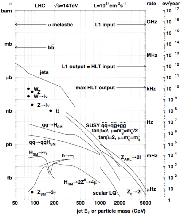
Figure 1: Production rates for the LHC. Figure from Ref. [2].

1.1.1 Data recording

The first LHC challenge is the sheer amount of data produced by ATLAS and CMS. The two proton beams cross each other every 25 ns or at 40 MHz, and a typical event consists of millions of detector channels, requiring 1.6 MB of memory. This data output of an LHC experiments corresponds to 1 PB per second. Triggering is another word for accepting that we cannot write all this information on tape and analyze is later, and we are also not interested in doing that. Most of the proton-proton interactions do not include any interesting fundamental physics information, so in the past we have just selected certain classes of events to write to tape. For model-driven searches this strategy was appropriate, but for our modern approach to LHC physics it is not. Instead, we should view triggering as some kind of data compression of the incoming LHC data, including compressing events, compressing event samples, or selecting events.

In Fig. 1 we see that between the inelastic proton-proton scattering cross section, or rate, of around 600 mb and hard jet production at a rate around $1~{}\mu$b we can afford almost a factor $10^{-6}$ in data reduction, loss-less when it comes to the fundamental physics questions we care about. This is why a first, level-one (L1) trigger can reduce the rate from an input rate of 40 MHz to an output rate around 100 kHz, without losing interesting physics, provided we make the right trigger decisions. To illustrate this challenge, the time a particle or a signal takes to cross a detector at the speed of light is

$$\frac{10~{}\text{m}}{3\cdot 10^{8}~{}\text{m/s}}\approx 3\cdot 10^{-8}~{}\text{s}=30~{}\text{ns}$$ (1.1)

or around one bunch-crossing time. As a starting point, the L1-trigger uses very simple and mostly local information from the calorimeters and the muon system, because at this level it is already hard to combine different regions of the detector in the L1 trigger decision. From a physics point of view this is a problem because events with two forward jets are very different depending on the question of they come with central jets as well. If yes, the event is likely QCD multi-jet production and not that interesting, if no, the event might be electroweak vector boson fusion and very relevant for many Higgs and electroweak gauge boson analyses.

After the L1 hardware trigger there is a second, software-based high-level (HL) or L2 trigger. It takes the L1 trigger output at 100 kHz and reduces the rate to 3 kHz, running on a dedicated CPU farm with more than 10.000 CPU cores already now. After that, for instance ATLAS runs an additional software-based L3 trigger, reducing the data rate from 3 kHz to 200 Hz. For 1.6 MB per event, this means that the experiment records 320 MB per second for the actual physics analyses. Following Fig. 1 a rate of 200 Hz starts to cut into Standard Model jet production, but covers the interesting SM processes as well as typical high-rate BSM signals (not that we believe that they describe nature).

This trigger chain defines the standard data acquisition by the LHC experiments and its main challenges related to the amount of information which needs to be analyzed. The big problem with triggering by selection is that it really is data compression with large losses, based on theoretical inspiration on interesting or irrelevant physics. Or in other words, if theorists are right, triggering by selection is lossless, but the track record of theorists in guessing BSM physics at the LHC is not a success story.

Even for Run 2 there were ways to circumvent the usual triggers and analyze data either by randomly choosing data to be written on tape (prescale trigger) or by performing analyses at the trigger level and without access to the full detector information (data scouting). One aspect that is, for instance, not covered by standard ATLAS and LHC triggers are low-mass di-jet resonances and BSM physics appearing inside jets. The prize we pay for this kind of event-level compression is that again it is not lossless, for instance when we need additional information to improve a trigger-level analysis later. Still, for instance LHCb is running a big program of encoding even analysis steps on programmable chips, FPGAs, to compress their data flow.

Before we apply concepts from modern data science to triggering we should once again think about what we really want to achieve. Reminding ourselves of the idea behind triggering, we can translate the trigger task into deep-learning language as one of two objectives,

• fast identification of events corresponding to a known, interesting class;

• fast identitication of events which are different from our Standard Model expectations;

• compress data such that it can be used best.

The first of these datasets can be used to measure, for example, Higgs properties, while the second dataset is where we search for physics beyond the Standard Model. As mentioned above, we can use compression strategies based on event selection, sample-wise compression, and event-level compression to deal with the increasingly large datasets of the coming LHC runs. Conceptually, it is more interesting to think about the anomaly-detection logic behind the second approach. While it is, essentially, a literal translation of the fundamental goal of the LHC to explore the limitations of the Standard Model and find BSM physics, is hardly explored in the classic approaches. We will see that modern data science provides us with concepts and tools to also implement this new trigger strategy.

1.1.2 Jet and event reconstruction

After recording an event, ATLAS and CMS translate the detector output into information on the particles which leave the interaction points, hadrons of all kind, muons, and electrons. Neutrinos can be reconstructed as missing transverse momentum, because in the azimuthal plane we know the momenta of both incoming partons.

To further complicate things, every bunch crossing at the HL-LHC consists of 150-200 overlapping proton-proton interactions. If we assume that one of them might correspond to an interesting production channel, like a pair of top quarks, a Higgs boson accompanied by a hard jet or gauge boson, or a dark matter particle, the remaining 149-199 interactions are refereed to as pileup and need to be removed. For this purpose we rely on tracking information for charged particles, which allow us to extrapolate particles back to the primary interaction point of the proton-proton collision we are interested in. Because the additional interaction of protons and of partons inside a proton, as well as soft jet radiation, do not have distinctive patterns, we can also get rid of them by subtracting unwanted noise for instance in the calorimeter. Denoising is a standard methodology used in data science for image analyses.

After reconstructing the relevant particles, the hadrons are clustered into jets, corresponding to hard quarks or gluons leaving the interaction points. These jets are traditionally defined by recursive algorithms, which cluster constituents into a jet using a pre-defined order and compute the 4-momentum of the jet which we use as a proxy for the 4-momentum of the quark of gluon produced in the hard interaction. The geometric separation of two LHC objects is defined in terms of the azimuthal angle $\phi_{ij}\in[0,\pi]$ and the difference in rapidity, $\Delta\eta_{ij}=|\eta_{i}-\eta_{j}|$. In the most optimistic scenario the LHC rapidity coverage is $|\eta_{i}|\lesssim 4.5$, for a decent jet reconstruction or $b$-jet identification is around $|\eta_{i}|\lesssim 2.5$. This 2-dimensional plane is what we would see if we unfolded the detector as viewed from the interaction point. We define the geometric separation in this $\eta-\phi$ plane as

$$R_{ij}=\sqrt{(\Delta\phi_{ij})^{2}+(\Delta\eta_{ij})^{2}}\;.$$ (1.2)

Jets can also be formed by hadronically decaying tau leptons or $b$-quarks, or even by strongly boosted, hadronically decaying $W$, $Z$, and Higgs bosons or top quarks. The top quark is the only quark that decays before it hadronizes. In all of these cases we need to construct the energy and momentum of the initial particle and its particle properties from the jet constituents, including the possibility that BSM physics might appear inside jets. Identifying the partonic nature of a jet is called jet tagging. The main information on jets comes from the hadronic and electromagnetic calorimeters, with limited resolution in the $\eta-\phi$ plane. The tracker adds more information at a much better angular resolution, but only for the charged particles in the jet. The combination of calorimeter and tracking information is often referred to as particle flow.

When relating jets of constituents we need to keep in mind a fundamental property of QFT: radiating a soft photon or gluon from a hard electron or quark can, in the limit $E_{\gamma,g}\to 0$, have no impact on any kinematic observable. Similarly, it cannot make a difference if we replace a single parton by a pair of partons arising from a collinear splitting. In both, the soft and collinear limits, the corresponding splitting probabilities described by QCD are formally divergent, and we have to resum these splittings to define a hard parton beyond leading order in perturbation theory. Because any detector has a finite resolution, and the calorimeter resolution is not even that good, these divergences are not a big problem for many standard LHC analyses, but when we define high-level kinematic observables to compare to QFT predictions, these observables should ideally be infrared and collinearly safe. An example for an unsafe observable is the number of particle-flow objects inside a jet.

Finally, details on jets only help us understand the underlying hard scattering through their correlations with other particles forming an event. This means we need to combine the subjet physics information inside a jet with correlations describing all particles in an event. This combination allows us, for instance to reconstructs a Higgs decaying to a pair of bottom quarks or a top decaying hadronically, $t\to W^{+}b\to jjb$, or leptonically $t\to W^{+}b\to\ell^{+}\nu b$. However, fundamentally interesting information requires us to understand complete events like for instance

$$pp\to t\bar{t}H+\text{jets}\to(jjb)\;(\ell^{-}\bar{\nu}\bar{b})\;(b\bar{b})+\text{jets}\;.$$ (1.3)

Again applying a deep-learning perspective, the reconstruction of LHC jets and events includes tasks like

• fast identification of particles through their detector signatures;

• data denoising to extract features of the relevant scattering;

• jet tagging and reconstruction using calorimeter and tracker;

• combination of low-level high-resolution with high-level low-resolution observables.

Event reconstruction and kinematic analyses have been using multivariate analysis methods for a very long time, with great success for example in $b$-tagging. Jet tagging is also the field of LHC physics where we are making the most rapid and transformative progress using modern machine learning, specifically classification networks. The switch to event-level tagging, on the other hand, is an unsolved problem.

1.1.3 Simulations

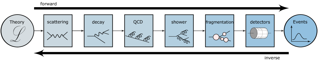
Figure 2: Illustrated simulation chain for LHC physics.

Simulations are the main way we provide theory predictions for the LHC experiments. A Lagrangian encodes the structures of the underlying quantum field theory. For the Standard Model this includes a $SU(3)\times SU(2)\times U(1)$ gauge group with the known fundamental particles, including one Higgs scalar. This theory describes all collider experiments until now, but leaves open cosmological questions like dark matter or the baryon asymmetry of the Universe, which at some point need to be included in our Lagrangian. It also ignores any kind of quantum gravity or cosmological constant. Because we use our LHC simulations not only for background processes, but also for potential signals, the input to an LHC simulation is the Lagrangian. This means we can simulate LHC events in any virtual world, provided we can describe it with a Lagrangian. From this Lagrangian we then extract known and new particles with their masses and all couplings. The universal simulation tools used by ATLAS and CMS are Pythia as the standard tool, Sherpa with its excellent QCD description, Madgraph with its unique flexibility for BSM searches, and Herwig with its excellent hadronization description.

The basic elements of the LHC simulation chain are illustrated in Fig. 2, and many more details can be found in Ref. [3]. Once we define our underlying theory Lagrangian, meaning the Standard Model without or with hypothetical new particles and interactions, we can compute the hard scattering amplitude. Following our $t\bar{t}H$ example in Eq.(1.3) the hard scattering can be defined in terms of top and Higgs, but if we want to include angular correlations in the top decays, the hard process will include the decays and include four $b$-quarks, a lepton, a neutrino, and two light-flavor quarks. If decaying particles contribute to such a phase space signature, we need to regularize the divergent on-shell propagators through a resummation which leads to a Breit-Wigner propagator and introduces a physical particle width to remove the on-shell divergence. Breit-Wigner propagators are one example for localized and strongly peaked feature in the matrix element as a function of phase space. In our $t\bar{t}H$ example process two top resonances, one Higgs resonance, and two $W$-resonances lead to numerical challenges in the phase space description, sampling, and integration. Finally, the transition amplitudes are computed in perturbative QCD. To leading order or at tree level, these amplitudes can be generated extremely fast by our standard generators. Nobody calculates those cross sections by hand anymore, and the techniques used by the automatic generators have little to do with the methods we tend to teach in our QFT courses. At the one-loop or 2-loop level things can still be automized, but the calculation of amplitudes including virtual QCD corrections and additional jet radiation can be time-consuming.

Moving on in Fig. 2, strongly interacting partons can radiate gluons and split off quarks into a collinear phase space. For instance looking at incoming gluons, they are described by parton densities beyond leading order in QCD only once we include this collinear radiation into the definition of the incoming gluons. The same happens for strongly interacting particles in the final state, referred to as fragmentation. For our reference process in Eq.(1.3) we are lucky in that heavy top quarks do not radiate many gluons. The universal initial and final state radiation, described by QCD beyond strict leading order gives rise to the additional jets indicated in Eq.(1.3). If we go beyond leading order in $\alpha_{s}$, we need to include hard jet radiation, which appears at the same order in perturbation theory as the virtual corrections. From a QFT-perspective virtual and real corrections lead to infrared-divergent predictions individually and therefore cannot be treated separately. More precise simulations in perturbation theory also lead to higher-multiplicity final states. From a machine learning perspective this means that LHC simulations cannot be defined in terms of a fixed phase-space dimensionality. In addition, it illustrates how for LHC simulation we can often exchange complexity and precision, which in return means that faster simulation tools are almost automatically more precise.

Hard initial-state and final-state radiation is only one effect of collinear and soft QCD splittings. The splitting of quarks and gluons into each other can be described fairly well by the 2-body splitting kernels, and these kernels describe the leading physics aspects of parton densities. In addition, successive QCD splittings define the so-called parton shower, which means they describes how a single parton with an energy of 100 GeV or more turns into a spray of partons with individual energies down to 1 GeV. There are several approaches to describing the parton shower, which share the simple set of QCD splitting kernels, but differ in the way the collinear radiation is spread out to fill the full phase space and in which order partons split. Improving the precision of parton showers to match the experimental requirements is one of the big challenges in theoretical LHC physics.

Next, the transition from quarks and gluons to mesons and baryons, and the successive hadron decays are treated by hadronization of fragmentation tools. From a QCD perspective those models are the weak spot of LHC simulations, because we are only slowly moving from ad-hoc models to first-principle QCD predictions. A precise theoretical description of many hadronization processes and hadron decays is challenging, so many features of hadron decays are extracted from data. Here we typically rely on the kinematic features of Breit-Wigner resonances combined with continuum spectra and form factors computed in low-energy QCD. The LHC simulation chain up to this point is developed and maintained by theorists.

The finally step in Fig. 2 is where the particles produced in LHC collisions enter the detectors and are analyzed by combining many aspects and channels of ATLAS, CMS, or LHCb. From a physics perspective detectors are described by the interaction of relativistic particles with the more or less massive different detector components. This interaction leads to electromagnetic and hadronic showers, which we need to describe properly if we want to simulate events based on a hypothetical Lagrangian. Because we do not expect to learn fundamental physics from the detector effects, and because detector effects depend on many details of the detector materials and structures, these simulations are in the hands of the experimental collaborations. The standard full simulations are based on the detailed construction plans of the detectors and use the complex and quite slow Geant4 tool for the full simulations. Fast simulations are based on these full simulations, ignore the input of the geometric detector information, and just reproduce the observed signals and measurements for a given particle entering the detector. Historically, they have relied on Gaussian smearing, but modern fast simulations are much more complex and precise.

If we are looking for deep-learning applications, first-principle simulations include challenges like

• optimal phase space coverage and mapping of amplitude features;

• fast and precise surrogate models for expensive loop amplitudes;

• variable-dimensional and high-dimensional phase spaces;

• improved data- and theory-driven hadron physics, like heavy-flavor fragmentation;

Once we can simulate LHC events all the way to the detector output, based on an assumed fundamental Lagrangian, and with high and controlled precision, we can use these simulated events to extract fundamental physics from LHC data. While not all LHC predictions can be included in this forward simulation, the multi-purpose event generators and the corresponding detector simulations are the work horses behind every single LHC analysis. They define LHC physics as much as the fact that the LHC collides two protons (or more), and there are infinitely many ways they can benefit from modern machine learning [4].

1.1.4 Inference

LHC analyses are almost exclusively based on frequentist or likelihood methods, and we are currently observing a slow transition from classic Tevatron-inherited analysis strategies to modern LHC analysis ideas. In an ideal LHC world, we would just compare observed events with simulated events based on a given theory hypothesis. From the Neyman-Pearson lemma we know that the likelihood ratio is the optimal way to compare two hypotheses and decide if a background-only model or a combined signal plus background model describes the observed LHC data better. This means we can assign any LHC dataset a confidence level for the agreement between observations and first-principle predictions and either discover or rule out BSM models with new particles and interactions. The theory-related assumption behind such analyses is that we can provide precise, flexible, and fast event generation for SM-backgrounds and for all signals we are interested in.

If we compare observed and predicted datasets, a key question is how we can set up the analysis such that it provides the best possible measurement. For two hypotheses the Neyman-Pearson lemma tells us that there exists a well-defined solution, because we can construct a likelihood-based observable which combines all available information into a sufficient statistics. The question is how we can first define and then experimentally reconstruct this optimal observable. Going back to our $t\bar{t}H$ example, we can for instance try to measure the top-Higgs Yukawa coupling. This coupling affects the signal rate simply as $\sigma_{\text{tot}}(t\bar{t}H)\propto y_{t}^{2}$ and does not change the kinematics of the signal process, so we can start with a simple $\bar{t}H$ rate measurement. Things get more interesting when we search for a modification of the top-Higgs couplings through a higher-dimensional operator, which changes the Lorentz structure of the coupling and introduces a momentum dependence. In that case the effect of a shifted coupling depends on the phase space position. Because the signal-to-background ratio also changes as a function of phase space, we need to find out which phase space regions work best to extract such an operator-induced coupling shift. The answer will depend on the luminosity, and we need an optimal observable framework to optimize such a full phase-space analysis. Finally, we can try to test fundamental symmetries in an LHC process, for instance the CP-symmetry of the top-Higgs Yukawa coupling. For this coupling, CP-violation would appear as a phase in the modified Yukawa coupling and affect the interference between different Feynman diagrams over phase space. Again, we can define an optimal observable for CP-violation, usually an angular correlation.

From a simulation point of view, illustrated in Fig. 2, the question of how to measure an optimal observable points to a structural problem. While we can assume that such an optimal observable is naturally defined at the parton or hard scattering level, the measurement has to work with events measured by the detector. The challenge becomes how to best link these different levels of the event generation and simulation to define the measurement of a Lagrangian parameter?

If we want to interpret measurements as model-independently as possible and in the long term, we need to report experimental measurements without detector effects. We can assume that the detector effects are independent on the fundamental nature of an event, so we translate a sample of detector-level events into a corresponding sample of events before detector effects and therefore entirely described by fundamental physics. From a formal perspective, we want to use a forward detector simulation to define a detector unfolding as an incompletely defined inverse problem.

Going back to Fig. 2 the possibility of detector unfolding leads to the next question, namely why we do not also unfold other layers of the simulation chain based on the assumption that they will not be affected by the kind of physics beyond the Standard Model we aim for. It is safe to assume that testing fragmentation models will not lead to a discovery of new particles, and the same can be argued (or not) for the parton shower. This is why it is standard to unfold or invert the shower and fragmentation steps of the forward simulations through the recursive jet algorithms mentioned before.

Next, it is reasonable to assume that BSM features like heavy new particles of momentum-dependent effective operators affect heavy particle production in specific phase space regions much more than the well-measured decays of gauge bosons or top quarks. For the $t\bar{t}H$ signal we would then not be interested in the top and Higgs decays, because they are affected with limited momentum transfer, and we can unfold these decays. This method is applied very successfully in the top groups of ATLAS and CMS, while other working groups are less technically advanced.

Finally, we can remind ourselves that what we really want to compute for any LHC process is a likelihood ratio. Modulo prefactors, the likelihood for a given process is just the transition amplitude for the hard process. This means that for example for two model or model-parameter hypotheses based on the same hard process, the likelihood ratio can be extracted easily by inverting the entire LHC simulation chain and extracting the parton-level matrix elements squared for a given observed events. This analysis strategy is called the matrix element method and has in the past been applied to especially challenging signals with small rates.

Altogether, simulation-based inference methods immediately bear the question how we want to compare simulation and data most precisely. If our simulation chain only works in the forward direction, we have no choice but to compare predictions and data at the event level. However, if our simulation chain can be inverted, we generate much more freedom. A very practical consideration might then also be that we are able to provide precision-QCD predictions for certain kinematic observables at the parton level, but not as part of a fast multi-purpose Monte Carlo. In this situation we can choose the point of optimal analysis along the simulation chain shown in Fig. 2.

In a data-oriented language some of the open questions related to modern LHC inference concern

• precision simulations of backgrounds and signals in optimized phase space regions;

• fast and precise event generation for flexible signal hypotheses;

• definition of optimal analysis strategies and optimal observables;

• unfolding or inverted forward simulation using a consistent statistical procedure;

• single-event likelihoods to be used in the matrix element method;

Many of these questions have a long history, starting from LEP and the Tevatron, but for the vast datasets of the LHC experiment we finally need to find conceptual solutions for a systematic inversion of our established and successful simulation chain.

1.1.5 Uncertainties

Uncertainties are extremely serious business in particle physics, because if we ever declare a major discovery we need to be sure that this statement lasts. We define, most generally, two kinds of uncertainties, statistical uncertainties and systematic uncertainties. The first kind is defined by the fact that they vanish for large statistics and are described by Poisson and eventually Gaussian distributions in any rate measurement. The second kind do not vanish with large statistics, because they come from some kind of reference measurement or calibration, because they describe detector effects, or they arise from theory predictions which do not offer a statistical interpretation. Some systematic uncertainties are Gaussian, for example when they describe a high-statistics measurement in a control region. Others just give a range and no preference for a single central value, for instance in the case of theory predictions based on perturbative QCD. Again, the distribution of the corresponding nuisance parameter reflects the nature of the systematic or theory uncertainties.

As a side remark, the machine learning distinguishes between two kinds of uncertainties, aleatoric uncertainties related to the (training) data and epistemic uncertainties related to the model we apply to describe the data. This separation is similar to statistical and systematic uncertainties. One of the issues is that we typically work towards the the limit of a perfectly trained network which reproduce all features of the data. Deviations from this limit are reproduced by the epistemic uncertainty, but the same limit requires increasingly large networks which we need to train on correspondingly large datasets.

Technically, we include uncertainties in a likelihood analysis using hundreds or thousands of nuisance parameters. Any statistical model for a dataset $x$ then depends on nuisance parameters $\nu$ and parameters of interest $\theta$, to define a likelihood $p(x|\nu,\theta)$. Instead of using Bayes’ theorem to extract a probability distribution $p(\theta|x,\nu)$, we use profile likelihood techniques to constrain $\theta$. These techniques do not foresee priors, unless we can describe them reliably as nuisance parameters reflecting measurements or theory predictions with a well-defined likelihood distribution. Whenever nuisance parameters come from a measurement, we expect their distribution to allow for a frequentist interpretations.

If we start with the assumption that the definition of an observable does not induce an uncertainty on the measurement, any observable will first be analyzed using simulations. Here we can ensure its resilience to detector effects, or, if needed, its appropriate QFT definition. In the current LHC strategy, any numerically defined observable, like a kinematic reconstruction, a boosted decision tree, or a neural network will actually be defined on simulated data. In the next step, this observable needs to be calibrated by combining data and simulations. A standard, nightmare task in ATLAS and CMS is the precise calibration of QCD jets. As a function of the many parameters of the jet algorithm this calibration will for instance determine the jet energy scale from controlled reference data like on-shell $Z$-production. Calibration can remove systematic biases, and it always comes with a range of uncertainties in the reference data, which include statistical limitations as well as theory uncertainties from the way the reference data is described by Monte Carlo simulations. We will see that for ML-based observables this second step can and should be considered part of the training, in which case the training has to account for uncertainties.

In the inference, we need to consider all kinds of uncertainties, together with the best choice of observables, to provide the optimal measurement. Because theory predictions are based on perturbative QFT, they always come with an uncertainty which we can sometimes quantify well, and which we sometimes know very little about. What we do know is that this theory uncertainty cannot be defined by a frequentist argument. Similarly, some systematic uncertainties are hard to estimate, for example when they correspond to detector effects which are not Gaussian or when we simply do not know the source of a bias for example in a calibration. Quantifying, controlling, and reducing all uncertainties is the challenge of any LHC analysis.

Finally, the uncertainty in defining an observable might not be part of the uncertainty treatment at the analysis level, but it will affect its optimality. This means that especially for numerically defined observable we need to control underlying uncertainty like the statistics of the training data, systematic affects related to the training, or theoretical aspects related to the definition of an observable. Historically, these uncertainties mattered less, but with the rapidly growing complexity of LHC data and analyses, they should be controlled.

This means that again in the language closer to machine learning we have to work on

• controlled definitions and resilience of observables;

• calibration leading to nuisance parameters for the uncertainty;

• control of the features learned by a neural network;

• uncertainties on all network outputs from classification to generation;

• balance optimal observables with uncertainties.

These requirements are, arguably, the biggest challenge in applying ML-methods to particle physics and the reason for conservative reservations especially in the ATLAS experiment. Given that we have no alternative to thinking of LHC physics as a field-specific application of data science, we have to work on the treatment of uncertainties in modern ML-techniques.

1.2 Deep learning

After setting the physics stage, we will briefly review some fundamental concepts which we need to then talk about machine learning at the LHC. We will not follow the usual line of many introductions to neural networks, but choose a particle physics path. This means we will introduce many concepts and technical terms using multivariate analyses and decision trees, then review numerical fits, and with that basis introduce neural networks with likelihood-based training. We will end this section with a state-of-the-art application of learning transition amplitudes over phase space.

1.2.1 Multivariate classification

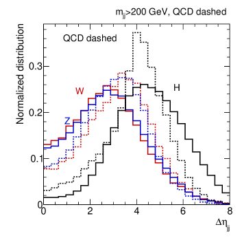
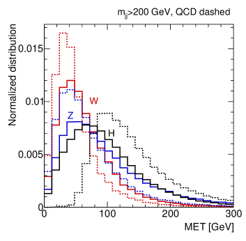
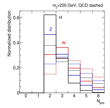
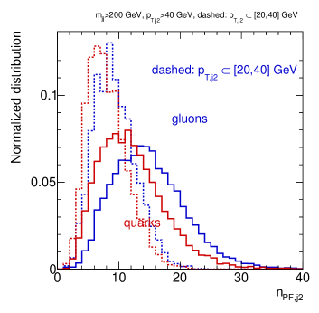
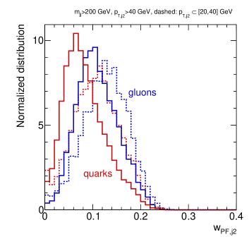
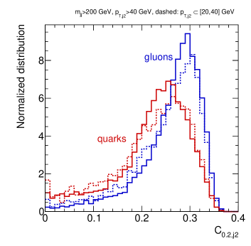
Figure 3: Sample distributions for the WBF kinematics (upper) and quark vs gluon discrimination (lower). Figures from Ref. [5].

Because LHC detector have a very large number of components, and because the relevant analysis questions involve many aspects of a recorded proton-proton collision, experimental analyses rely on a large number of individual measurements. We can illustrate this multi-observable strategy with a standard classification task, the identification of invisible Higgs decays as a dark matter signature. The most promising production process to look for this Higgs decay is weak boson fusion, so our signature consists of two forward tagging jets and missing transverse momentum from the decaying Higgs,

$$qq^{\prime}\to(H\to\text{inv})\;qq^{\prime}\qquad\text{or}\qquad pp\to(H\to\text{inv})\;jj+\text{jets}\;.$$ (1.4)

Following Fig. 2 we start with a $2\to 3$ hard scattering, where the Higgs decay products cannot be observed, two forward tagging jets with high energy and transverse momenta around $p_{T}\sim 30~{}...~{}150$ GeV, and the key feature that the additional jets in the signal process are not central because of fundamental QCD considerations [3]. The main background is $Z$+jets production, where the $Z$ decays to two neutrinos. A typical set of basic kinematic cuts at the event level is

$$p_{T,j_{1,2}} >40\,\text{GeV} \qquad\qquad\qquad|\eta_{j_{1,2}}| <4.5 \qquad\qquad\qquad\hbox to0.0pt{\hbox to7.95831pt{\hfil/\hfil}\hss}E_{T} >140\,\text{GeV}$$

$$\eta_{j_{1}}\;\eta_{j_{2}} <0 |\Delta\eta_{jj}| >3.5 m_{jj} >600\,\text{GeV}$$

$$p_{T,j_{3}} >20\,\text{GeV} \qquad\qquad\qquad|\eta_{j_{3}}| <4.5 \text{(if 3rd jet there)}\;.$$ (1.5)

On the sub-jet level we can exploit the fact that the electroweak signal only includes quark jets, whereas the background often features one gluon in the final state. Kinematic subjet variables which allow us to distinguish quarks from gluons based on particle-flow (PF) objects are

$$n_{\text{PF}} =\sum_{i_{\text{PF}}}1 \qquad\qquad\qquad w_{\text{PF}} =\frac{\sum_{i_{\text{PF}}}\;p_{T,i}\;\Delta R_{i,\text{jet}}}{\sum_{i_{\text{PF}}}\;p_{T,i}}$$

$$p_{T}D =\frac{\sqrt{\sum_{i_{\text{PF}}}\;p_{T,i}^{2}}}{\sum_{i_{\text{PF}}}p_{T,i}} \qquad\qquad\qquad C =\frac{\sum_{i_{\text{PF}},j_{\text{PF}}}\;p_{T,i}p_{T,j}\;\left(\Delta R_{ij}\right)^{0.2}}{\left(\sum_{i_{\text{PF}}}p_{T,i}\right)^{2}}\;.$$ (1.6)

Altogether, there is a sizeable number of kinematic observables which help us extract the signal. They are shown in Fig. 3, and the main message is that none of them has enough impact to separate signal and background on its own. Instead, we need to look at correlations between these observables, including correlations between event-level and subjet observables. Examples for such correlations would be the rapidity of the third jet, $\eta_{j3}$ as a function of the separation of the tagging jets, $\Delta\eta_{jj}$, and combined with the quark or gluon nature of the tagging jets. More formally, what we need is a method to classify events based on a combination of many observables.

As a side remark we can ask why we should limit ourselves to the set of theory-defined observables in Eq.(1.5) and Eq.(1.6). When looking at classification with neural networks in Sec. 2 we will see that modern machine learning allows us to instead use preprocessed calorimeter output, but for now we will stick to the standard, high-level observables in Eqs.(1.5) and (1.6).

To target correlated observables, multivariate classification is an established problem in particle physics. The classical solution for it are or used to be a decision tree. Imagine we want to classify an event $x_{i}$ into the signal or background category based on a set of observables $\mathcal{O}_{j}$. As a basis for this decision we study a sample of training events $\{x_{i}\}$, histogram them for each observable $\mathcal{O}_{j}$, and find the values $\mathcal{O}_{j,\text{split}}$ which give the most successful split between signal and background for each distribution. To define such an optimal split we start with the signal and background probabilities or so-called impurities as a function of the signal event count $S$ and the background event count $B$,

$$p_{S}=\frac{S}{S+B}\equiv p\qquad\qquad\text{and}\qquad\qquad p_{B}=\frac{B}{S+B}\equiv 1-p\;.$$ (1.7)

These probabilities will allow us to define optimal cuts. If we look at a histogrammed normalized observable $\mathcal{O}\in[0~{}...~{}1]$ we can compute $p$ and $1-p$ from number of expected signal and background events following Eq.(1.7). For instance, we can look at a signal which prefers large $\mathcal{O}$-values two background distributions and first compute the signal and background probabilities $p(\mathcal{O})$. We can then decide that a single event is signal-like when its (signal) probability is $p(\mathcal{O})>1/2$, otherwise the event is background,

$$S(\mathcal{O}) =A\mathcal{O} \qquad\qquad B(\mathcal{O}) =A(1-\mathcal{O}) \quad\Rightarrow\quad p(\mathcal{O}) =\mathcal{O} \quad\Rightarrow\quad\mathcal{O}_{\text{split}} =\frac{1}{2}$$

$$S(\mathcal{O}) =A\mathcal{O} \qquad\qquad B(\mathcal{O}) =B \quad\Rightarrow\quad p(\mathcal{O}) =\frac{\mathcal{O}}{\mathcal{O}+\dfrac{B}{A}} \quad\Rightarrow\quad\mathcal{O}_{\text{split}} =\frac{B}{A}\;.$$ (1.8)

The appropriate or optimal splitting point for each observable is then given by

$$\mathcal{O}_{j,\text{split}}=\mathcal{O}_{j}\Big{|}_{p=1/2}\;.$$ (1.9)

To organize our multivariate analysis we then need to evaluate the performance of each optimized cut $\mathcal{O}_{j,\text{split}}$, for example to apply the most efficient cut first or at the top of a decision tree.

For such a construction we start with a a sample $\{x\}$ of events, distributed according to the true or data distribution $p_{\text{data}}(x)$. We then construct a model approximating the true distribution in terms of the model parameters $\theta$, called $p_{\text{model}}(x|\theta)$. Evaluated as a function of $\theta$, the probability distribution $p_{\text{model}}(x|\theta)$ defines a likelihood, and it should agree with $p_{\text{data}}(x)$. The Neyman-Pearson lemma also tells us that the ratio of the two likelihoods is the most powerful test statistic to distinguish the two underlying hypotheses, defined as the smallest false negative error for a given false positive rate. One way to compare two distributions is through the Kullback-Leibler divergence

$$\boxed{D_{\text{KL}}[p_{\text{data}},p_{\text{model}}]=\Bigg{\langle}\log\frac{p_{\text{data}}}{p_{\text{model}}}\Bigg{\rangle}_{p_{\text{data}}}\equiv\int dx\;p_{\text{data}}(x)\;\log\frac{p_{\text{data}}(x)}{p_{\text{model}}(x|\theta)}}\;.$$ (1.10)

It vanishes if two distributions agree everywhere, and we postpone the inverse direction of this argument to Sec. 4. Because the KL-divergence is not symmetric in its two arguments we can evaluate two versions,

$$D_{\text{KL}}[p_{\text{model}},p_{\text{data}}]=\Bigg{\langle}\log\frac{p_{\text{model}}}{p_{\text{data}}}\Bigg{\rangle}_{p_{\text{model}}}\qquad\text{or}\qquad D_{\text{KL}}[p_{\text{data}},p_{\text{model}}]=\Bigg{\langle}\log\frac{p_{\text{data}}}{p_{\text{model}}}\Bigg{\rangle}_{p_{\text{data}}}\;.$$ (1.11)

The first is called forward KL-divergence, the second one is the reverse KL-divergence. The difference between them is which of the two distributions we choose to sample the logarithm from, forward is sampled from simulation, backward is sampled from data, just as one would assume for a forward and an inverse problem. Of the two versions we can choose the KL-divergence which suits us better, and since we are working on an existing, well-defined training dataset it makes sense to use the second definition to find the best values of $\theta$ and make sure our NN-model approximates the training data well,

$$D_{\text{KL}}[p_{\text{data}},p_{\text{model}}]=\Bigg{\langle}\log\frac{p_{\text{data}}(x)}{p_{\text{model}}(x|\theta)}\Bigg{\rangle}_{p_{\text{data}}} =\big{\langle}\log p_{\text{data}}(x)\big{\rangle}_{p_{\text{data}}}-\big{\langle}\log p_{\text{model}}(x|\theta)\big{\rangle}_{p_{\text{data}}}$$

$$=-\big{\langle}\log p_{\text{model}}(x|\theta)\big{\rangle}_{p_{\text{data}}}+\text{const}(\theta)\;.$$ (1.12)

We want to minimize the log-likelihood ratio or KL-divergence as a function of the model parameters $\theta$, so we can ignore the second term and instead work with the so-called cross entropy instead,

$$H[p_{\text{data}},p_{\text{model}}] :=-\big{\langle}\log p_{\text{model}}(x|\theta)\big{\rangle}_{p_{\text{data}}}$$

$$\equiv-\sum_{\{x\}}\;p_{\text{data}}(x)\log p_{\text{model}}(x|\theta)\;.$$ (1.13)

As a probability distribution $p_{\text{model}}(x|\theta)\in[0,1]$, so $H[p_{\text{data}},p_{\text{model}}]>0$. If we construct $p_{\text{model}}(x|\theta)$ by minimizing a KL-divergence or the cross entropy, we refer to the minimized function as the loss function, sometimes also called objective function. The second term in Eq.(1.12) only ensures that the target value of the loss function is zero.

If we want reproduce several distributions simultaneously we can generalize the cross entropy to

$$H[\vec{p}_{\text{data}},\vec{p}_{\text{model}}] =-\sum_{j}\big{\langle}\log p_{\text{model},j}(x|\theta)\big{\rangle}_{p_{\text{data},j}}\equiv-\sum_{j}\sum_{\{x\}}\;p_{\text{data},j}(x)\log p_{\text{model},j}(x|\theta)\;.$$ (1.14)

As a sum of individual cross entropies it becomes minimal when each of the $p_{\text{model},j}$ approximates its respective $p_{\text{data},j}$, unless there is some kind of balance to be found between non-prefect approximations. For signal vs background classification, we want to reproduce the signal and the background distributions defined in Eq.(1.7), giving us the 2-class or 2-label cross entropy

$$H[\vec{p}_{\text{data}},\vec{p}_{\text{model}}] =-\big{\langle}\log p_{\text{model}}(x|\theta)\big{\rangle}_{x\sim p_{\text{data}}}-\big{\langle}\log\left(1-p_{\text{model}}(x|\theta)\right)\big{\rangle}_{x\sim 1-p_{\text{data}}}$$

$$\equiv-\sum_{\{x\}}\;\Big{[}p_{\text{data}}\log p_{\text{model}}+(1-p_{\text{data}})\log(1-p_{\text{model}})\Big{]}\;.$$ (1.15)

To clarify the sampling we again give the actual definition in the second line. We remind ourselves that we need to minimize two conditions simultaneously, $p_{\text{data}}$ and $1-p_{\text{data}}$, with their approximations $p_{\text{model}}$ and $1-p_{\text{model}}$. In cases where we understand the data and know that the simulated and measured histograms agree well, $p\equiv p_{\text{model}}=p_{\text{data}}$, the cross entropy simplifies to

$$H[\vec{p},\vec{p}]=-\sum_{\{x\}}\;\Big{[}p\log p+(1-p)\log(1-p)\Big{]}\;.$$ (1.16)

The simplified cross entropy vanishes for zero for $p=0$ and $p=1$ and is symmetric around the maximum at $H[p=1/2]=\log 2$. This corresponds to the fact that for perfectly understood datasets with only $p(x)=0$ and $p(x)=1$ this entropy as a measure for our ignorance vanishes. If we change the formula in Eq.(1.16) to $\log_{2}$, which means $H[p=1/2]\to 1$, the cross entropy tells us how many bits or how much information we need to say if an event $x$ in a given dataset is signal or background. We will come back to the minimization of the cross entropy and the likelihood ratio in Sec. 4.2.1.

After all this discussion on comparing probability densities, we rephrase Eq.(1.9) in terms of the cross entropy as

$$\mathcal{O}_{j,\text{split}}=\text{argmax}_{\text{splits}}H[\vec{p}(\mathcal{O}),\vec{p}(\mathcal{O})]\;.$$ (1.17)

This argument works for any function with a maximum at $p=1/2$, but the cross entropy will serve another purpose. As mentioned above, to build a decision tree out of our observables we need to compute the best splitting for each observable individually and then choose the observable with the most successful split. To quantify this performance we can follow the argument that a large cross entropy means an impure sample which requires a lot of information to determine if an event is a signal. If we know the cross entropy values for the two subsets after the split we want them both to be as small as possible. More precisely, we want to maximize the difference of the cross entropy before the split and the sum of the cross entropies after the split, called the information gain. This means we choose the observable on top of the decision tree though

$$\max_{j}\Big{[}H_{\text{before split}}[\vec{p},\vec{p}]-H_{\text{after split},1}[\vec{p},\vec{p}]-H_{\text{after split},2}[\vec{p},\vec{p}]\Big{]}\;.$$ (1.18)

A historic illustration for a decision tree used in particle physics is shown in the left panel of Fig. 4. It comes from the first high-visibility application of (boosted) decision trees in particle physics, to identify electron-neutrinos from a beam of muon-neutrinos using the MiniBooNE Cerenkov detector. Each observable defines a so-called node, and the two branches below each node are defined as ‘yes’ vs ‘no’ or as ‘signal-like’ vs ‘background-like’. The first node is defined by the observable with the highest information gain among all the optimal splits. The two branches are based on this optimal split value, found by maximizing the cross entropy. Every outgoing branch defines the next node again through the maximum information gain, and its outgoing branches again reflect the optimal split, etc. Finally, the algorithm needs a condition when we stop splitting a branch by defining a node and instead define a so-called leaf, for instance calling all events ‘signal’ after a certain number of splittings selecting it as ‘signal-like’. Such conditions could be that all collected training events are either signal or background, that a branch has too few events to continue, or simply by enforcing a maximum number of branches.

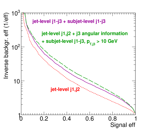
Figure 4: Left: illustration of a decision tree from an early application in particle physics, selecting electron neutrinos to prove neutrino oscillations. Figure from Ref. [6]. Right: signal efficiency vs background rejection for WBF Higgs production and invisible Higgs decays, based on jet-level and additional subjet-level information shown in Tab. 1. Figure from Ref. [5].

No matter how we define the stopping criterion for constructing a decision tree, there will always be signal events in background leaves and vice versa. We can only guarantee that a tree is completely right for the training sample, if each leaf includes one training event. This perfect discrimination obviously does not carry over to an independent test sample, which means our decision tree is overtrained. In general, overtraining means that the performance for instance of a classifier on the training data is so finely tuned that it follows the statistical fluctuations of the training data and does not generalize to the same performance on independent sample of test data.

If we want to further enhance the performance of the decision tree we can focus on the events which are wrongly classified after we define the leaves. For instance, we can add an event weight $w>1$ to every mis-identified event (we care about) and carry this weight through the calculation of the splitting condition. This is the simple idea behind a boosted decision tree (BDT). Usually, the weights are chosen such that the sum of all events is one. If we construct several independent decision trees, we can also combine their output for the final classifier. It is not obvious that this procedure will improve the tree for a finite number of leaves, and it is not obvious that such a re-weighting will converge to a unique or event improved boosted decision tree, but in practice this method has been shown to be extremely powerful.

Set		Variables
jet-level $j_{1}$, $j_{2}$		$p_{T,j_{1}}\quad p_{T,j_{2}}\quad\Delta\eta_{jj}\quad\Delta\phi_{jj}\quad m_{jj}\quad\hbox to0.0pt{\hbox to7.16249pt{\hfil/\hfil}\hss}E_{T}\quad\Delta\phi_{j_{1},\hbox to0.0pt{\hbox to5.01373pt{\hfil/\hfil}\hss}E_{T}}\quad\Delta\phi_{j_{2},\hbox to0.0pt{\hbox to5.01373pt{\hfil/\hfil}\hss}E_{T}}$
subjet-level $j_{1}$, $j_{2}$		$n_{\text{PF},j_{1}}\quad n_{\text{PF},j_{2}}\quad p_{T}D_{j_{1}}\quad p_{T}D_{j_{2}}\quad C_{j_{1}}\quad C_{j_{2}}$
$j_{3}$ angular information		$\Delta\eta_{j_{1},j_{3}}\quad\Delta\eta_{j_{2},j_{3}}\quad\Delta\phi_{j_{1},j_{3}}\quad\Delta\phi_{j_{2},j_{3}}$
jet-level $j_{1}$-$j_{3}$		jet-level $j_{1}$, $j_{2}$  $+$  $j_{3}$ angular information  $+$  $p_{T,j_{3}}$
subjet-level $j_{1}$-$j_{3}$		subjet-level $j_{1}$, $j_{2}$  $+$  $n_{\text{PF},j_{3}}\quad C_{j_{3}}\quad p_{T}D_{j_{3}}$

Table 1: Sets of variables used in a BDT study for a WBF Higgs search with invisible Higgs decays. The subscript $jj$ refers to the two tagging jets, not all events have a third jet. Example from Ref. [5].

Finally, we need to measure the performance of a BDT classification using some kind of success metric. Obviously, a large signal efficiency alone is not sufficient, because the signal-to-background ratio $S/B$ or the Gaussian significance $S/\sqrt{B}$ depend on the signal and background rates. For a simple classification task we can compute four numbers

1. signal efficiency, or true positive rate $\epsilon_{S}\equiv S^{\text{(S-tagged)}}/S^{\text{(truth)}}$;

2. background efficiency, or true negative rate $B^{\text{(B-tagged)}}/B^{\text{(truth)}}$;

3. background mis-identification rate, or false positive rate $\epsilon_{B}\equiv B^{\text{(S-tagged)}}/B^{\text{(truth)}}$;

4. signal mis-identification rate, or false negative rate $S^{\text{(B-tagged)}}/S^{\text{(truth)}}$.

If we tag all events we know the normalization conditions $S^{\text{(truth)}}=S^{\text{(S-tagged)}}+S^{\text{(B-tagged)}}$ and correspondingly for $B^{\text{(truth)}}$. The signal efficiency is also called recall or sensitivity in other fields of research. The background mis-identification rate can be re-phrased as background rejection $1-\epsilon_{B}$, also referred to as specificity. Once we have tagged a signal sample we can ask how many of those tagged events are actually signal, defining the purity or precision $S^{\text{(S-tagged)}}/(S^{\text{(S-tagged)}}+B^{\text{(S-tagged)}})$. Finally, we can ask how many of our decisions are correct and compute $(S^{\text{(S-tagged)}}+B^{\text{(B-tagged)}})/(S^{\text{(truth)}}+B^{\text{(truth)}})$.

In particle physics we usually measure the success of a classifier in the plane $\epsilon_{S}$ vs $\epsilon_{B}$, where for the latter we either write $1-\epsilon_{B}$ of $1/\epsilon_{B}$. In the right panel of Fig. 4 we show such a plane for our invisible Higgs decay example. It is called receiver–operator characteristics (ROC) curve. The different sets of observables are shown in Tab. 1. The lowest ROC curve corresponds to a BDT analysis of the kinematic observables of the two tagging jets and the missing transverse energy vector. For a signal efficiency $\epsilon_{S}=40\%$ it gives a background rejection around $1/\epsilon_{B}=1/10$. If we expect a relatively large signal rate and at the same time need to reject the background more efficiently, we can choose a different working point of the classifier, for instance $\epsilon_{S}=20\%$ and $1/\epsilon_{B}=1/35$.

If a classifier gives us, for example, a continuous measure of signal-ness of an event being signal we can choose different working points by defining a cut on the classifier output. The problem with such any such cut is that we lose information from all those signal events which almost made it to the signal-tagged sample. If we can construct our classifier such that its output is a probability, we can also weight all events by their signal vs background probability score and keep all events in our analysis.

Going back to LHC physics, in Fig. 4 we see that adding information on the potential third jet and subjet observables for all three jets with the additional requirement of $p_{T,j}>10$ GeV improves the background rejection for $\epsilon_{S}=40\%$ to almost $1/\epsilon_{B}=1/20$. Adding information from softer jets only has a small effect. Such ROC curves are the standard tool for benchmarking LHC analyses, reducing them to single performance values like the integral under the ROC curve (AUC) or the background rejection for a given signal efficiency is usually an oversimplification.

To summarize, data analysis without multivariate classification is hard to imagine for particle physicists. Independent of the question if we want to call boosted decision trees machine learning or not, we have shown how they can be constructed or trained for multivariate classification tasks, and we have taken the opportunity to define many technical terms we will need later in these notes. The great advantage of decision trees, in addition to the great performance of BDTs, is that we can follow their definition of signal and background regions fairly easily. We can always look at graphics like the one in the left panel of Fig. 4, at least before boosting, and standard tools like TMVA provide a list of the most powerful observables. The biggest disadvantage of decision trees is that by construction they do not account for correlations properly, they only break up the observable space into many rectangular leaves.

1.2.2 Fits and interpolations

From a practical perspective, we start with the assumption or observation that neural network are nothing but numerically defined functions. As alluded to in the last section, some kind of minimization algorithm on a loss function will allow us to define determine its underlying parameters $\theta$. The simplest case, regression networks are scalar or vector fields defined on some space, approximated by $f_{\theta}(x)$. Assuming that we have indirect or implicit access to the truth $f(x)$ in form of a training dataset $(x,f)_{j}$, we want to construct the approximation

$$\boxed{f_{\theta}(x)\approx f(x)}\;.$$ (1.19)

Usually, approximating a set of functional values for a given set of points can be done two ways. First, in a fit we start with a functional form in terms of a small set of parameters which we also refer to as $\theta$. To determine these model parameters, we maximize the probability for the fit output $f(x_{j})$ to correspond to the training points $f_{j}$, with uncertainties $\sigma_{j}$. This means we maximize the Gaussian likelihood

$$p(x|\theta) =\prod_{j}\frac{1}{\sqrt{2\pi}\sigma_{j}}\exp\left(-\frac{|f_{j}-f_{\theta}(x_{j})|^{2}}{2\sigma_{j}^{2}}\right)$$

$$\Rightarrow\qquad\log p(x|\theta) =-\sum_{j}\frac{|f_{j}-f_{\theta}(x_{j})|^{2}}{2\sigma_{j}^{2}}+\text{const}(\theta)\;.$$ (1.20)

In the Gaussian limit this log-likelihood is often referred to as $\chi^{2}$. In this form the individual Gaussians have mean $f_{j}$, a variance $\sigma_{j}^{2}$, a standard deviation $\sigma_{j}$, and a width of the bell curve of $2\sigma_{j}$. For the definition of the best parameters $\theta$ we can again ignore the $\theta$-independent normalization. The loss function for our fit, i.e.  the function we minimize to determine the fit’s model parameters is

$$\boxed{\mathcal{L}_{\text{fit}}=\sum_{j}\mathcal{L}_{j}=\sum_{j}\frac{|f_{j}-f_{\theta}(x_{j})|^{2}}{2\sigma_{j}^{2}}}\;.$$ (1.21)

The fit function is not optimized to go though all or even some of the training data points, $f_{\theta}(x_{j})\neq f_{j}$. Instead, the log-likelihood loss is a compromise to agree with all training data points within their uncertainties. We can plot the values $\mathcal{L}_{j}$ for the training data and should find a Gaussian distribution of mean zero and standard deviation one, $\mathcal{N}_{\mu=0,\sigma=1}$.

An interesting question arises in cases where we do not know an uncertainty $\sigma_{j}$ for each training point, or where such an uncertainty does not make any sense, because we know all training data points to the same precision $\sigma_{j}=\sigma$. In that case we can still define a fit function, but the loss function becomes a simple mean squared error,

$$\mathcal{L}_{\text{fit}}=\frac{1}{2\sigma^{2}}\sum_{j}|f_{j}-f_{\theta}(x_{j})|^{2}\equiv\frac{1}{2\sigma^{2}}\text{MSE}\;.$$ (1.22)

Again, the prefactor is $\theta$-independent and does not contribute to the definition of the best fit. This simplification means that our MSE fit puts much more weight on deviations for large functional values $f_{j}$. This is often not what we want, so alternatively we could also define the loss in terms of relative uncertainties. In practical applications of machine learning we will instead apply preprocessings of the data,

$$f_{j}\to\log f_{j}\qquad\text{or}\qquad f_{j}\to f_{j}-\langle f_{j}\rangle\qquad\text{or}\qquad f_{i}\to\frac{f_{i}}{\langle f_{i}\rangle}\cdots$$ (1.23)

In cases where we expect something like a Gaussian distribution a standard scaling would preprocess the data to a mean of zero and a standard deviation of one. In an ideal world, such preprocessings should not affect our results, but in reality they almost always do. The only way to avoid preprocessings is to add information like the scale of expected and allowed deviations for the likelihood loss in Eq.(1.21).

The second way of approximating a set of functional values is interpolation, which ensures $f_{\theta}(x_{j})=f_{j}$ and is the method of choice for datasets without noise. Between these training data points we choose a linear or polynomial form, the latter defining a so-called spline approximation. It provides an interpolation which is differentiable a certain number of times by matching not only the functional values $f_{\theta}(x_{j})=f_{j}$, but also the $n$th derivatives $f_{\theta}^{(n)}(x\uparrow x_{j})=f_{\theta}^{(n)}(x\downarrow x_{j})$. In the machine learning language we can say that the order of our spline defines an implicit bias for our interpolation, because it defines a resolution in $x$-space where the interpolation works. A linear interpolation is not expected to do well for widely spaced training points and rapidly changing functional values, while a spline-interpolation should require fewer training points because the spline itself can express a non-trivial functional form.

The main difference between a fit and an interpolation is their respective behavior on unknown dataset. For both, a fit and an interpolation we expect our model $f_{\theta}(x)$ to describe the training data. To measure the quality of a fit beyond the training data we can compute the loss function $\mathcal{L}$ or the point-wise contributions to the loss $\mathcal{L}_{j}$ on an independent test dataset. If a fit does not generalize from a training to a test dataset, it is usually because it has learned not only the smooth underlying function, but also the statistical fluctuation of the training data. While a test dataset of the same size will have statistical fluctuations of the same size, they will not be in the same place, which means the loss function evaluated on the training data will be much smaller than the loss function evaluated on the test data. This failure mode is called over-fitting or, more generally, overtraining. For interpolation this overtraining is a feature, because we want to reproduce the training data perfectly. The generalization property is left to choice of the interpolation function. As a side remark, manipulating the training dataset while performing one fit after the other is an efficient way to search for outliers in a dataset, or a new particle in an otherwise smooth distribution of invariant masses at the LHC.

More systematically, we can define a set of errors which we make when targeting a problem by constructing a fit function through minimizing a loss on a training dataset. First, an approximation error is introduced when we define a fit function, which limits the expressiveness of the network in describing the true function we want to learn. Second, an estimation or generalization error appears when we approximate the true training objective by a combination of loss function and training data set. In practice, these errors are related. A justified limit to the expressiveness of a fit function, or implicit bias, defines useful fits for a given task. In many physics applications we want our fit to be smooth at a given resolution. When defining a good fit, increasing the class of functions the fit represents leads to a smaller approximation error, but increases the estimation error. This is called the bias-variance trade off, and we can control it by limiting or regularizing the expressiveness of the fit function and by ensuring that the loss of an independent test dataset does not increase while training on the training dataset. Finally, any numerical optimization comes with a training error, representing the fact that a fitted function might just live, for instance, in a sufficiently good local minimum of the loss landscape. This error is a numerical problem, which we can solve though more efficient loss minimization. While we can introduce these errors for fits, they will become more relevant for neural networks.

1.2.3 Neural networks

One way to think about a neural network is as a numerically defined fit function, often with a huge number of model parameters $\theta$, and written just like the fit of Eq.(1.19),

$$f_{\theta}(x)\approx f(x)\;.$$ (1.24)

As mentioned before, we minimize a loss function numerically to determine the neural network parameters $\theta$. This procedure us called network training and requires a training dataset $(x,f)_{j}$ representing the target function $f(x)$. To control and avoid overtraining, we can compare the values of the loss function between the training dataset and an independent test dataset.

We will skip the usual inspiration from biological neurons and instead ask our first question, which is how to describe an unknown function in terms of a large number of model parameters $\theta$ without making more assumptions than some kind of smoothness on the relevant scales. For a simple regression task We can write the mapping as

$$x\to f_{\theta}(x)\qquad\text{with}\quad x\in\mathbb{R}^{D}\quad\text{and}\quad f_{\theta}\in\mathbb{R}\;.$$ (1.25)

The key is to think of this problem in terms of building blocks which we can put together such that simple functions require a small number of modules or building blocks, and model parameters, and complex functions require larger and larger numbers of those building blocks. We start by defining so-called layers, which in a fully connected or dense network transfer information from all $D$ entries of the vector $x$ defining one layer to all vector entries of the layer to its left,

$$x\to x^{(1)}\to x^{(2)}\cdots\to x^{(N)}\equiv f_{\theta}(x)$$ (1.26)

Counting the input $x$ this means our network consist of $N+1$ layers, including one input layer, one output layer, and $N-1$ hidden layers. If a vector entry $x_{j}^{(n+1)}$ collects information from all $x^{(n)}_{j}$, we can try to write each step of this chain as

$$x^{(n-1)}\to x^{(n)}:=W^{(n)}x^{(n-1)}+b^{(n)}\;,$$ (1.27)

where the $D\times D$ matrix $W$ is referred to as the network weights and the $D$-dimensional vector $b$ as the bias. In general, neighboring layers do not need to have the same dimension, which means $W$ does not have to be a diagonal matrix. In our simple regression case we already know that over the layers we need to reduce the width of the network from the input vector dimension $D$ to the output scalar $x^{(N)}=f_{\theta}(x)$.

Splitting the vector $x^{(n)}$ into its $D$ entries defines the nodes which form our network layer

$$x_{i}^{(n)}=W_{ij}^{(n)}x_{j}^{(n-1)}+b_{i}^{(n)}\;.$$ (1.28)

For a fully connected network a node takes $D$ components $x_{j}^{(n-1)}$ and transforms them into a single output $x_{i}^{(n)}$. For each node the $D+1$ network parameters are $D$ matrix entries $W_{ij}$ and one bias $b_{i}$. If we want to compute the loss function for a given data point $(x_{j},f_{j})$, we follow the arrows in Eq.(1.26), use each data point as the input layer, $x=x_{j}$, go through the following layers one by one, compute the network output $f_{\theta}(x_{j})$, and compare it to $f_{j}$ though a loss function.

The transformation shown in Eq.(1.27) is an affine transformation. Just like linear transformations, affine transformations form a group. This is equivalent to saying that combining affine layers still gives us an affine transformation, just encoded in a slightly more complicated manner. This means our network defined by Eq.(1.27) can only describe linear functions, albeit in high-dimensional spaces.

To describe non-linear functions we need to introduce some kind of non-linear structure in our neural network. The simplest implementation of the required nonlinearity is to apply a so-called activation function to each node. Probably the simplest 1-dimensional choice is the so-called rectified linear unit

$$\text{ReLU}(x_{j}):=\max(0,x_{j})=\begin{cases}0&x_{j}\leq 0\\ x_{j}&x_{j}>0\end{cases}\;,$$ (1.29)

giving us instead of Eq.(1.28)

$$\boxed{x^{(n-1)}\to x^{(n)}:=\text{ReLU}\left[W^{(n)}x^{(n-1)}+b^{(n)}\right]}\;,$$ (1.30)

Here we write the ReLU transformation of a vector as the vector of ReLU-transformed elements. This non-linear transformation is the same for each node, so all our network parameters are still given by the affine transformations. But now a sufficiently deep network can describe general, non-linear functions, and combining layers adds complexity, new parameters, and expressivity to our network function $f_{\theta}(x)$. There are many alternatives to ReLU as the source of non-linearity in the network setup, and depending on our problem they might be helpful, for example by providing a finite gradient over the $x$-range. However, throughout this lecture we always refer to a standard activation function as ReLU.

This brings us to the second question, namely, how to determine a correct or at least good set of network parameters $\theta$ to describe a training dataset $(x,f)_{j}$. From our fit discussion we know that one way to determine the network or model parameters is by minimizing a loss function. For simplicity, we can think of the MSE loss defined in Eq.(1.22) and ignore the normalization $1/(2\sigma^{2})$. To minimize the loss we have to compute its derivative with respect to the model parameters. If we ignore the bias for now, for a given weight in the last network layer we need to compute

$$\frac{d\mathcal{L}}{dW^{(N)}_{1j}} =\frac{\partial\left|f-\text{ReLU}[W^{(N)}_{1k}x^{(N-1)}_{k}]\right|^{2}}{\partial\text{ReLU}[W^{(N)}_{1k}x^{(N-1)}_{k}]}\;\frac{\partial\text{ReLU}[W^{(N)}_{1k}x^{(N-1)}_{k}]}{\partial[W^{(N)}_{1k}x^{(N-1)}_{k}]}\;\frac{\partial[W^{(N)}_{1k}x^{(N-1)}_{k}]}{\partial W^{(N)}_{1j}}$$

$$=-2\left|f-\text{ReLU}[W^{(N)}_{1k}x^{(N-1)}_{k}]\right|\times 1\times\delta_{jk}x^{(N-1)}_{k}$$

$$\equiv-2\sqrt{\mathcal{L}}\;x^{(N-1)}_{j}\;,$$ (1.31)

provided $W^{(N)}_{ij}x_{j}>0$, otherwise the partial derivative vanishes. This form implies that the derivative of the loss with respect to the weights in the $N$th layer is a function of the loss itself and of the previous layer $x^{(N-1)}$. If we ignore the ReLU derivative in Eq.(1.31) and still limit ourselves to the weight matrix in Eq.(1.30) we can follow the chain of layers and find

$$\frac{d\mathcal{L}}{dW^{(n)}_{ij}} =\frac{\partial\left|f-\text{ReLU}[W^{(N)}_{1k}x^{(N-1)}_{k}]\right|^{2}}{\partial[W^{(N)}_{1k}x^{(N-1)}_{k}]}\;\frac{\partial[(W^{(N)}\cdots W^{(n+1)})_{1k}W^{(n)}_{k\ell}x^{(n-1)}_{\ell}}{\partial W^{(n)}_{ij}}$$

$$=-2\sqrt{\mathcal{L}}\;\left(W^{(N)}\cdots W^{(n+1)}\right)_{1i}x_{j}^{(n-1)}\;.$$ (1.32)

This means we compute the derivative of the loss with respect to the weights in the reverse direction as the network evaluation shown in Eq.(1.26). We have shown this only for the network weights, but it works for the biases the same way. This back-propagation is the crucial step in defining appropriate network parameters by numerically minimizing a loss function. The simple back-propagation might also give a hint to why the chain-like network structure of Eq.(1.26) combined with the affine layers of Eq.(1.27) have turned out so successful as a high-dimensional representation of arbitrary functions.

The output of the back-propagation in the network training is the expectation value of the derivative of the loss function with respect to a network parameter. While we could evaluate this expectation value over the full training dataset. Especially for large datasets, it becomes impossible to compute this expectation value, so instead we evaluate the same expectation value over a small, randomly chosen subset of the training data. This method is called stochastic gradient descent, and the subsets of the training data are called minibatches or batches

$$\Bigg{\langle}\frac{\partial\mathcal{L}}{\partial\theta_{j}}\Bigg{\rangle}_{\text{minibatch}}\qquad\text{with}\quad\theta_{j}\in\{b,W\}\;.$$ (1.33)

Even through the training data is split into batches and the network training works on these batches, we still follow the progress of the training and the numerical value of the loss as a function of epochs, defined as the number of batch trainings required for the network to evaluate the full training sample.

After showing how to compute the loss function and its derivative with respect to the model parameters, the final question is how we actually do the minimization. For a given network parameter $\theta_{j}$, we first need to scan over possible values widely, and then tune it precisely to its optimal value. In other words, we first scan the parameter landscape globally, identify the global minimum or at least a local minimum close enough in loss value to the global minimum, and then descend into this minimum. This is a standard task in physics, including particle physics, and compared to many applications of Markov Chains Monte Carlos the standard ML-minimization is not very complicated. We start with the naive iterative optimization in time steps

$$\theta_{j}^{(t+1)}=\theta_{j}^{(t)}-\alpha\Bigg{\langle}\frac{\partial\mathcal{L}^{(t)}}{\partial\theta_{j}}\Bigg{\rangle}\;.$$ (1.34)

The minus sign means that our optimization walks against the direction of the gradient, and $\alpha$ is the learning rate. From our description above it is clear that the learning rate should not be constant, but should follow a decreasing schedule.

One of the problems with the high-dimensional loss optimization is that far away from the minimum the gradients are small and not reliable. Nevertheless, we know that we need large steps to scan the global landscape. Once we approach a minimum, the gradients will become larger, and we want to stay within the range of the minimum. An efficient adaptive strategy is given by

$$\theta_{j}^{(t+1)}=\theta_{j}^{(t)}-\alpha\frac{\Big{\langle}\dfrac{\partial\mathcal{L}^{(t)}}{\partial\theta_{j}}\Big{\rangle}}{\epsilon+\sqrt{\Big{\langle}\dfrac{\partial\mathcal{L}^{(t)}}{\partial\theta_{j}}\Big{\rangle}^{2}}}\;.$$ (1.35)

Away from the minimum, this form allows us to enhance the step size even for small gradients by choosing a sizeable value $\alpha$. However, whenever the gradient grows too fast, the step size remains below the cutoff $\alpha/\epsilon$. Finally, we can stabilize the walk through the loss landscape by mixing the loss gradient at the most recent step with gradients from the updates before,

$$\Bigg{\langle}\frac{\partial\mathcal{L}^{(t)}}{\partial\theta_{j}}\Bigg{\rangle}\;\to\;\beta\Bigg{\langle}\frac{\partial\mathcal{L}^{(t)}}{\partial\theta_{j}}\Bigg{\rangle}+(1-\beta)\Bigg{\langle}\frac{\partial\mathcal{L}^{(t-1)}}{\partial\theta_{j}}\Bigg{\rangle}$$ (1.36)

This strategy is called momentum, and now the complicated form of the denominator in Eq.(1.35) makes sense, and serves as a smoothing of the denominator for rapidly varying gradients. A slightly more sophisticated version of this adaptive scan of the loss landscape is encoded in the widely used Adam optimizer.

Note that for any definition of the step size we still need to schedule the learning rate $\alpha$. A standard choice for such a learning rate scheduling is an exponential decay of $\alpha$ with the batch or epoch number. An interesting alternative is a one-cycle learning rate where we first increase $\alpha$ batch after batch, with a dropping loss, until the loss rapidly explodes. This point defines the size of the minimum structure in the loss landscape. Now we can choose the step size at the minimum loss value to define a suitable constant learning rate for our problem, potentially leading to much faster training. Finally, we need to mention that the minimization of the loss function for a neural network only ever uses first derivatives, differently from the optimization of a fit function. The simple reason is that for the large number of network parameters $\theta$ the simple scaling of the computational effort rules out computing second derivatives like we would normally do.

Going back to the three error introduced in the last section, they can be translated directly to neural networks. The approximation error is less obvious than for the choice of fit function, but also the expressiveness of neural network is limited through the network architecture and the set of hyperparameters. The training error becomes more relevant because we now minimize the loss over an extremely high-dimensional parameter space, where we cannot expect to find the global minimum and will always have to settle for a sufficiently good local minimum. To define a compromise between the approximation and generalization errors we usually divide a ML-related dataset into three parts. The main part is the training data, anything between 60% and 80% of the data. The above-mentioned test data is then 10% to 20% of the complete dataset, and we use it to check how the network generalizes to unseen data, test for overtraining, or measure the network performance. The validation data can be used to re-train the network, optimize the architecture or the different settings of the network. The crucial aspect is that the test data is completely independent of the network training.

1.2.4 Bayesian networks and likelihood loss

After we have understood how we can construct and train a neural network in complete analogy to a fit, let us discuss what kind of network we actually need for simple physics applications. We start from the observation that in a scientific application we are not only interested in single network output or a set of network parameters $\theta$, but need to include the corresponding uncertainty. Going back to fits, any decent fit approach provides error bands for each of the fit parameters, ideally correlated. With this uncertainty aspect in mind, a nice and systematic approach are so-called Bayesian neural networks. This kind of network is a naming disaster in that there is nothing exclusively Bayesian about them [7], while in particle physics Bayesian has a clear negative connotation. The difference between a deterministic and a Bayesian network is that the latter allow for distributions of network parameters, which then define distributions of the network output and provide central values $f(x)$ as well as uncertainties $\Delta f(x)$ by sampling over $\theta$-space. The corresponding loss function follows a clear statistics logic in terms of a distribution of network parameters.

Let us start with a simple regression task, computing the a scalar transition amplitude as a function phase space points,

$$f_{\theta}(x)\approx f(x)\equiv A(x)\qquad\text{with}\quad x\in\mathbb{R}^{D}\;.$$ (1.37)

The training data consists of pairs $(x,A)_{j}$. We define $p(A)\equiv p(A|x)$ as the probability distribution for possible amplitudes at a given phase space point $x$ and omit the argument $x$ from now on. The mean value for the amplitude at the point $x$ is

$$\langle\,A\,\rangle=\int dA\;A\;p(A)\qquad\text{with}\qquad p(A)=\int d\theta\;p(A|\theta)\;p(\theta|x_{\text{train}})\;.$$ (1.38)

Here $p(\theta|x_{\text{train}})$ are the network parameter distributions and $x_{\text{train}}$ is the training dataset. We do not know the closed form of $p(\theta|x_{\text{train}})$, because it is encoded in the training data. Training the network means that we approximate it as a distribution using variational approximation for the integrand in the sense of a distribution and test function

$$p(A)=\int d\theta\;p(A|\theta)\;p(\theta|x_{\text{train}})\approx\int d\theta\;p(A|\theta)\;q(\theta|x)\equiv\int d\theta\;p(A|\theta)\;q(\theta)\;.$$ (1.39)

As for $p(A)$ we omit the $x$-dependence of $q(\theta|x)$. This approximation leads us directly to the BNN loss function. We define the variational approximation using the Kullback-Leibler divergence introduced in Eq.(1.10),

$$D_{\text{KL}}[q(\theta),p(\theta|x_{\text{train}})]=\Bigg{\langle}\log\frac{q(\theta)}{p(\theta|x_{\text{train}})}\Bigg{\rangle}_{q}=\int d\theta\;q(\theta)\;\log\frac{q(\theta)}{p(\theta|x_{\text{train}})}\;.$$ (1.40)

There are many ways to compare two distributions, defining a problem called optimal transport. We will come back to alternative ways of combining probability densities over high-dimension spaces in Sec. 4. Using Bayes’ theorem we can write the KL-divergence as

$$D_{\text{KL}}[q(\theta),p(\theta|x_{\text{train}})] =\int d\theta\;q(\theta)\;\log\frac{q(\theta)p(x_{\text{train}})}{p(\theta)p(x_{\text{train}}|\theta)}$$

$$=D_{\text{KL}}[q(\theta),p(\theta)]-\int d\theta\;q(\theta)\;\log p(x_{\text{train}}|\theta)+\log p(x_{\text{train}})\int d\theta\;q(\theta)\;.$$ (1.41)

The prior $p(\theta)$ describes the model parameters before training. The model evidence $p(x_{\text{train}})$ guarantees the correct normalization of $p(\theta|x_{\text{train}})$ and is usually intractable. If we implement the normalization condition for $q(\theta)$ by construction, we find

$$D_{\text{KL}}[q(\theta),p(\theta|x_{\text{train}})] =D_{\text{KL}}[q(\theta),p(\theta)]-\int d\theta\;q(\theta)\;\log p(x_{\text{train}}|\theta)+\log p(x_{\text{train}})\;.$$ (1.42)

The log-evidence in the last term does not depend on $\theta$, which means that it will not be adjusted during training and we can ignore when constructing the loss. However, it ensures that $D_{\text{KL}}[q(\theta),p(\theta|x_{\text{train}})]$ can reach its minimum at zero. Alternatively, we can solve the equation for the evidence and find

$$\log p(x_{\text{train}}) =D_{\text{KL}}[q(\theta),p(\theta|x_{\text{train}})]-D_{\text{KL}}[q(\theta),p(\theta)]+\int d\theta\;q(\theta)\;\log p(x_{\text{train}}|\theta)$$

$$>\int d\theta\;q(\theta)\;\log p(x_{\text{train}}|\theta)-D_{\text{KL}}[q(\theta),p(\theta)]$$ (1.43)

This condition is called the evidence lower bound (ELBO), and the evidence reaches this lower bound exactly when our training condition in Eq.(1.10) is minimal. Combining all of this, we turn Eq.(1.42) or, equivalently, the ELBO into the loss function for a Bayesian network,

$$\boxed{\mathcal{L}_{\text{BNN}}=-\int d\theta\;q(\theta)\;\log p(x_{\text{train}}|\theta)+D_{\text{KL}}[q(\theta),p(\theta)]}\;.$$ (1.44)

The first term of the BNN loss is a likelihood sampled according to $q(\theta)$, the second enforces a (Gaussian) prior. This Gaussian prior acts on the distribution of network weights. The network output is constructed in a non-linear way with a large number of layers, to we can assume that Gaussian weight distributions do not limit us in terms of the uncertainty on the network output. The log-likelihood $\log p(x_{\text{train}}|\theta)$ implicitly includes the sum over all training points. At this stage we emphasize that from a practical perspective a good prior can help the network converge more efficiently, but any prior should give the correct results and we always need to test the effect of different priors.

Before we discuss how we evaluate the Bayesian network in the next section, we want to understand more about the BNN setup and loss. First, let us look at the deterministic limit of our Bayesian network loss. This means we want to look at the loss function of the BNN in the limit

$$q(\theta)=\delta(\theta-\theta_{0})\;.$$ (1.45)

The easiest way to look at this limit is to first assume a a Gaussian form of the network parameter distributions, as given in Eq.(1.20)

$$q_{\mu,\sigma}(\theta)=\frac{1}{\sqrt{2\pi}\sigma_{q}}e^{-(\theta-\mu_{q})^{2}/(2\sigma_{q}^{2})}\;,$$ (1.46)

and correspondingly for $p(\theta)$. The KL-divergence has a closed form,

$$D_{\text{KL}}[q_{\mu,\sigma}(\theta),p_{\mu,\sigma}(\theta)] =\frac{\sigma_{q}^{2}-\sigma_{p}^{2}+(\mu_{q}-\mu_{p})^{2}}{2\sigma_{p}^{2}}+\log\frac{\sigma_{p}}{\sigma_{q}}\;.$$ (1.47)

We can now evaluate this KL-divergence in the limit of $\sigma_{q}\to 0$ and finite $\mu_{q}(\theta)\to\theta_{0}$ as the one remaining $\theta$-dependent parameter,

$$D_{\text{KL}}[q_{\mu,\sigma}(\theta),p_{\mu,\sigma}(\theta)]\to\frac{(\theta_{0}-\mu_{p})^{2}}{2\sigma_{p}^{2}}+\text{const}\;.$$ (1.48)

We can write down the deterministic limit of Eq.(1.44),

$$\boxed{\mathcal{L}_{\text{BNN}}=-\log p(x_{\text{train}}|\theta_{0})+\frac{(\theta_{0}-\mu_{p})^{2}}{2\sigma_{p}^{2}}}\;.$$ (1.49)

While the first terms is again the likelihood defining the correct network parameters, the second terms ensures that network parameters do not become too large. Because it include the squares of the network parameters, it is referred to as an L2-regularization. While for the Bayesian network the prefactor of this regularization term is fixed, we can generalize this idea and apply an L2-regularization to any network with an appropriately chosen pre-factor.

Sampling the likelihood following a distribution of the network parameters, as it happens in the first term of the Bayesian loss in Eq.(1.44), is something we can also generalize to deterministic networks. Let us start with a toy model where we sample over network parameters by either including them in the loss computation or not. When we include an event, the network weight is set to $\theta_{0}$, otherwise $q(\theta)=0$. Such a random sampling between two discrete possible outcomes is described by a Bernoulli distribution. If the two possible outcomes are zero and one, we can write the distribution in terms of the expectation value $\rho\in[0,1]$,

$$P_{\text{Bernoulli},\rho}(x)=\rho^{x}(1-\rho)^{1-x}\qquad\text{for}\quad x=0,1\;.$$ (1.50)

We can include it as a test function for our integral over the log-likelihood $\log p(x_{\text{train}}|\theta)$ and find for the corresponding loss

$$\mathcal{L}=-\int dx\;\left[\rho^{x}(1-\rho)^{1-x}\right]_{x=0,1}\;\log p(x_{\text{train}}|\theta)=-\rho\;\log p(x_{\text{train}}|\theta_{0})$$ (1.51)

Such an especially simple sampling of weights by removing nodes it called dropout and is commonly used to avoid overfitting of networks. For deterministic networks $\rho$ is a free hyperparameter of the network training, while for Bayesian networks this kind of sampling is a key result from the construction of the loss function.

1.2.5 Amplitude regression

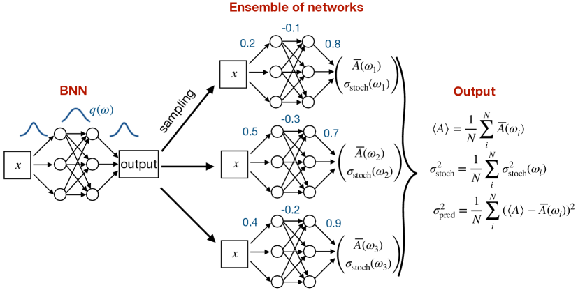
Figure 5: Illustration of a Bayesian network. Figure from Ref. [8].

After training the Bayesian network using its likelihood loss in Eq.(1.44) we still have to extract the mean and the uncertainty for the predicted function, in this case the amplitude $A$ over phase space. To evaluate the network we first exchange the two integrals in Eq.(1.38) and use the variational approximation to write the mean prediction $\overline{A}$ for a given phase space point as

$$\langle A\rangle =\int dAd\theta\;A\;p(A|\theta)\;p(\theta|x_{\text{train}})$$

$$=\int dAd\theta\;A\;p(A|\theta)\;q(\theta)$$

$$\equiv\int d\theta\;q(\theta)\;\overline{A}(\theta)\qquad\qquad\text{with $\theta$-dependent mean}\qquad\overline{A}(\theta)=\int dA\;A\;p(A|\theta)\;.$$ (1.52)

We can interpret this formula as a sampling over network parameters, provided we assume uncorrelated variations of the individual network parameters. Strictly speaking, this is an assumption we make. For a network with perfect $x$-resolution or perfect interpolation properties we can replace $q(\theta)\to\delta(\theta-\theta_{0})$, so $p(A|\theta)$ returns the one correct value for the amplitude. For noisy or otherwise limited training the probability distribution $p(A|\theta)$ describes a spectrum of amplitude labels for each phase space point. Corresponding to the definition of the $\theta$-dependent mean $\overline{A}$, the variance of $A$ is

$$\sigma_{\text{tot}}^{2} =\int dAd\theta\;\left(A-\langle A\rangle\right)^{2}\;p(A|\theta)\;q(\theta)$$

$$=\int dAd\theta\;\left(A^{2}-2A\langle A\rangle+\langle A\rangle^{2}\right)\;p(A|\theta)\;q(\theta)$$

$$=\int d\theta\;q(\theta)\left[\int dA\;A^{2}\;p(A|\theta)-2\langle A\rangle\;\int dA\;Ap(A|\theta)+\langle A\rangle^{2}\;\int dA\;p(A|\theta)\right]$$ (1.53)

For the three integrals we can generalize the notation for the $\theta$-dependent mean as in Eq.(1.52) and write

$$\sigma_{\text{tot}}^{2} =\int d\theta\;q(\theta)\left[\overline{A^{2}}(\theta)-2\langle A\rangle\overline{A}(\theta)+\langle A\rangle^{2}\right]$$

$$=\int d\theta\;q(\theta)\left[\overline{A^{2}}(\theta)-\overline{A}(\theta)^{2}+\overline{A}(\theta)^{2}-2\langle A\rangle\overline{A}(\theta)+\langle A\rangle^{2}\right]$$

$$=\int d\theta\;q(\theta)\left[\overline{A^{2}}(\theta)-\overline{A}(\theta)^{2}+\left(\overline{A}(\theta)-\langle A\rangle\right)^{2}\right]\equiv\sigma_{\text{stoch}}^{2}+\sigma_{\text{pred}}^{2}\;.$$ (1.54)

For this transformation we keep in mind that $\langle A\rangle$ is already integrated over $\theta$ and $A$ and can be pulled out of the integrals. This expression defines two contributions to the variance or uncertainty. First, $\sigma_{\text{pred}}$ is defined in terms of the $\theta$-integrated expectation value $\langle A\rangle$

$$\sigma_{\text{pred}}^{2} =\int d\theta\;q(\theta)\;\Big{[}\overline{A}(\theta)-\langle A\rangle\Big{]}^{2}\;.$$ (1.55)

Following the definition in Eq.(1.52), it vanishes in the limit of perfectly narrow network weights, $q(\theta)\to\delta(\theta-\theta_{0})$. If we assume precise training data, this limit also requires perfect training, which means that $\sigma_{\text{pred}}$ decreases with more and better training data. In that sense it represents a statistical uncertainty. In contrast, $\sigma_{\text{stoch}}$ already occurs without sampling the network parameters and does not vanish for $q(\theta)\to\delta(\theta-\theta_{0})$

$$\sigma_{\text{stoch}}^{2}\equiv\langle\sigma_{\text{stoch}}(\theta)^{2}\rangle =\int d\theta\;q(\theta)\;\sigma_{\text{stoch}}(\theta)^{2}$$

$$=\int d\theta\;q(\theta)\;\Big{[}\overline{A^{2}}(\theta)-\overline{A}(\theta)^{2}\Big{]}\;.$$ (1.56)

While this uncertainty receives contributions for instance from too little training data, it only approaches a plateau for perfect training. This plateau value can reflect a stochastic training sample, limited expressivity of the network, not-so-smart choices of hyperparameters etc, in the sense of a systematic uncertainty. To avoid mis-understanding we can refer to it as a stochastic or as model-related uncertainty,

$$\sigma_{\text{stoch}}\equiv\sigma_{\text{model}}\equiv\langle\sigma_{\text{model}}(\theta)^{2}\rangle\;.$$ (1.57)

To understand these two uncertainty measures better, we can look at the $\theta$-dependent network output and read Eq.(1.52) and (1.56) as the Bayesian network sampling $\overline{A}(\theta)$ and $\sigma_{\text{model}}(\theta)^{2}$ over a network parameter distribution $q(\theta)$ for each phase space point $x$

$$\boxed{\text{BNN}:x,\theta\to\begin{pmatrix}\overline{A}(\theta)\\ \sigma_{\text{model}}(\theta)\end{pmatrix}}\;.$$ (1.58)

If we follow Eq.(1.44) and assume $q(\theta)$ to be Gaussian, we now have a network with twice as many parameters as a standard network to describe two outputs. For a given phase space point $x$ we can then compute the three global network predictions $\langle A\rangle$, $\sigma_{\text{model}}$, and eventually $\sigma_{\text{pred}}$. Unlike the distribution of the individual network weights $q(\theta)$, the amplitude output is not Gaussian.

The evaluation of a BNN is illustrated in Fig. 5. From that graphics we see that a BNN works very much like an ensemble of networks trained on the same data and producing a spread of outputs. The first advantage over an ensemble is that the BNN is only twice as expensive as a regular network, and less if we assume that the likelihood loss leads to an especially efficient training. The second advantage of the BNN is that it learns a function and its uncertainty together, which will give us some insight into how advanced networks learn such densities in Sec. 4.3.3. The disadvantage of Bayesian networks over ensembles is that the Bayesian network only cover local structures in the loss landscape.

While we usually do not assume a Gaussian uncertainty on the Bayesian network output, this might be a good approximation for $\sigma_{\text{model}}(\theta)$. Using this approximation we can write the likelihood $p(x_{\text{train}}|\theta)$ in Eq.(1.44) as a Gaussian and use the closed form for the KL-divergence in Eq.(1.47), so the BNN loss function turns into

$$\mathcal{L}_{\text{BNN}} =\int d\theta\;q_{\mu,\sigma}(\theta)\;\sum_{\text{points $j$}}\left[\frac{\left|\overline{A}_{j}(\theta)-A_{j}^{\text{truth}}\right|^{2}}{2\sigma_{\text{model},j}(\theta)^{2}}+\log\sigma_{\text{model},j}(\theta)\right]$$

$$+\frac{\sigma_{q}^{2}-\sigma_{p}^{2}+(\mu_{q}-\mu_{p})^{2}}{2\sigma_{p}^{2}}+\log\frac{\sigma_{p}}{\sigma_{q}}\;.$$ (1.59)

As always, the amplitudes and $\sigma_{\text{model}}$ are functions of phase space $x$. The loss is minimized with respect to the means and standard deviations of the network weights describing $q(\theta)$. This interesting aspect of this loss function is that, while the training data just consists of amplitudes at phase space points and does not include the uncertainty estimate, the network constructs a point-wise uncertainty from the variation of the network parameters. This means we can rely on a well-defined likelihood loss rather than some kind of MSE loss even for our regression network training, this is fudging genius!

For some applications we might want to use this advantage of the BNN loss in Eq.(1.59), but without sampling the network parameters $\theta$. In complete analogy to a fit we can then use a deterministic network like in Eq.(1.47), described by $q(\theta)=\delta(\theta-\theta_{0})$ inserted into the Gaussian BNN loss in Eq.(1.59) to define

$$\mathcal{L}_{\text{heterostedastic}}=\sum_{\text{points $j$}}\left[\frac{\left|\overline{A}_{j}(\theta_{0})-A_{j}^{\text{truth}}\right|^{2}}{2\sigma_{\text{model},j}(\theta_{0})^{2}}+\log\sigma_{\text{model},j}(\theta_{0})\right]+\frac{(\theta_{0}-\mu_{p})^{2}}{2\sigma_{p}^{2}}\;.$$ (1.60)

The interplay between the first two terms works in a way that the first term can be minimized either by reproducing the data and minimizing the numerator, or by maximizing the denominator. The second term penalizes the second strategy, defining a correlated limit of $\overline{A}$ and $\sigma_{\text{model}}$ over phase space. Compared to the full Bayesian network this simplified approach has two disadvantages: first, we implicitly assume that the uncertainty on the amplitudes is Gaussian. Second, $\sigma_{\text{model}}$ only captures noisy amplitude values in the training data. Extracting a statistical uncertainty, as encoded in $\sigma_{\text{pred}}$, requires us to sample over the weight space. Obviously, this simplification cannot be interpreted as an efficient network ensembling.

For a specific task, let us look at LHC amplitudes for the production of two photons and a jet [9],

$$gg\to\gamma\gamma g(g)$$ (1.61)

The corresponding transition amplitude $A$ is a real function over phase space, with the detector-inspired kinematic cuts

$$p_{T,j} >20~{}\text{GeV} \qquad\qquad\qquad|\eta_{j}| <5 \qquad\qquad\qquad R_{jj,j\gamma,\gamma\gamma}>0.4$$

$$p_{T,\gamma} >40,30~{}\text{GeV} \qquad\qquad\qquad|\eta_{\gamma}| <2.37\;.$$ (1.62)

The jet 4-momenta are identified with the gluon 4-momenta through a jet algorithm. The standard computer program for this calculation is called NJet, and the same amplitudes can also be computed with the event generator Sherpa at one loop. This amplitude has to be calculated at one loop for every phase space point, so we want to train a network once to reproduce its output much faster. Because these amplitude calculations are a key ingredient to the LHC simulation chain, the amplitude network needs to reproduce the correct amplitude distributions including all relevant features and with a reliable uncertainty estimate.

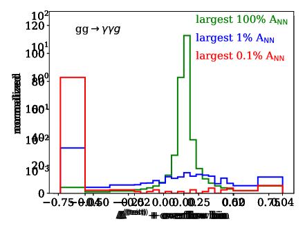
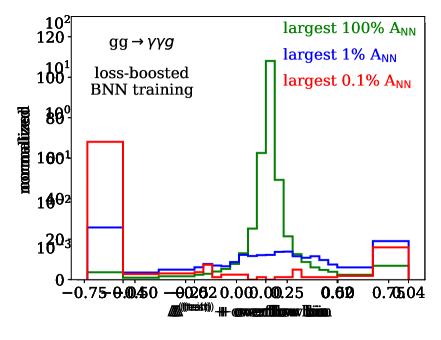
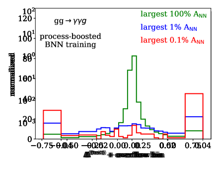
Figure 6: Performance of the BNN, loss-boosted BNN, and process-boosted BNN, in terms of the precision of the generated amplitudes, defined in Eq.(1.63) and evaluated on the training (upper) and test datasets. Figures from Ref. [10].

For one gluon in the final state, the most general phase space has $5\times 4=20$ dimensions. We could simplify this phase space by requiring momentum conservation and on-shell particles in the initial and final state, but for this test we leave these effects for the network to be learned. Limiting ourselves to one jet, this means we train a regression network to learn a real number over a 20-dimensional phase space. To estimate the precision of the network we can compute the relative deviation between the training or test data with the network amplitudes,

$$\Delta_{j}^{\text{(train/test)}}=\frac{\langle A\rangle_{j}-A_{j}^{\text{train/test}}}{A_{j}^{\text{train/test}}}$$ (1.63)

In the upper left panel of Fig. 6 we show the performance of a well-trained Bayesian network in reproducing the training dataset. While the majority of phase space points are described very precisely, a problem occurs for the phase space points with the largest amplitudes. The reason for this shortcoming is that there exist small phase space regions where the transition amplitude increase rapidly, by several orders of magnitude. The network fails to learn this behavior in spite of a $\log$-scaling following Eq.(1.23), because the training data in these regions is sparse. For an LHC simulation this kind of bias is a serious limitation, because exactly these phase space regions need to be controlled for a reliable rate prediction. This defines our goal of an improved amplitude network training, namely to identify and control outliers in the $\Delta$-distribution of Eq.(1.63).

The likelihood loss in Eq.(1.59) with its $\sigma_{\text{model}}(\theta)$ has a great advantage, because we can test the required Gaussian shape of the corresponding pull variable for the truth and NN-amplitudes,

$$\frac{\overline{A}_{j}(\theta)-A_{j}^{\text{truth}}}{\sigma_{\text{model},j}(\theta)}\;,$$ (1.64)

as part of the training. For the initial BNN run it turns out that this distribution indeed looks like a Gaussian in the peak region, but with too large and not exponentially suppressed tails. We can improve this behavior using an inspiration from the boosting of a decision tree. We enhance the impact of critical phase space points through an increased event weight, leading us to a boosted version of the BNN loss,

$$\mathcal{L}_{\text{BBNN}} =\int d\theta\;q_{\mu,\sigma}(\theta)\;\sum_{\text{points $j$}}n_{j}\times\left[\frac{\left|\overline{A}_{j}(\theta)-A_{j}^{\text{truth}}\right|^{2}}{2\sigma_{\text{model},j}(\theta)^{2}}+\log\sigma_{\text{model},j}(\theta)\right]$$

$$+\frac{\sigma_{q}^{2}-\sigma_{p}^{2}+(\mu_{q}-\mu_{p})^{2}}{2\sigma_{p}^{2}}+\log\frac{\sigma_{p}}{\sigma_{q}}\;.$$ (1.65)

This boosted or feedback training will improve the network performance both, in the precision of the amplitude prediction and in the learned uncertainty on the network amplitudes. If we limit ourselves to self-consistency arguments, we can select the amplitudes with $n_{j}>1$ through large pull values, as defined in Eq.(1.64). It turns out that this loss-based boosting significantly improves the uncertainty estimate. However, in the upper right panel of Fig. 6 we see that the effect on the large amplitudes is modest, large amplitudes still lead to too many outliers in the network precision, and we also tend to systematically underestimate those large amplitudes.

To further improve the performance of our network we can target the problematic phase space points directly, by increasing $n_{j}$ based on the size of the amplitudes. This process-specific boosting goes beyond the self-consistency of the network and directly improves a specific task beyond just learning the distribution of amplitudes over phase space. In the lower panels of Fig. 6 we see that at least for the training data the $\Delta$-distribution looks the same for small and large amplitudes. Going back to Eq.(1.2.2), we can interpret the boosted loss for large values of $n_{j}$ as a step towards interpolating the corresponding amplitudes. While for small amplitudes the network still corresponds to a fit, we are forcing the network to reproduce the amplitudes at some phase space points very precisely. Obviously, this boosting will lead to issues of overtraining. We can see this in the lower right panel of Fig. 6, where the improvement through process boosting for the test dataset does not match the improvement for the training dataset. However, as long as the performance of the test dataset improves, even if it is less than for the training dataset, we improve the network in spite of the overtraining. The issue with this overtraining is that it becomes harder to control the uncertainties, which might require some kind of alternating application of loss-based and process boosting.

This example illustrates three aspects of advanced regression networks. First, we have seen that a Bayesian network allows us to construct a likelihood loss even if the training data does not include an uncertainty estimate. Second, we can improve the consistency of the network training by boosting events selected from the pull distribution. Third, we can further improve the network through process-specific boosting, where we force the network from a fit to an interpolation mode based on a specific selection of the input data. For the latter the benefits do not fully generalize from the training to the test dataset, but the network performance does improve on the test dataset, which is all we really require.

1.2.6 Parton density regression

A peculiar and challenging feature of hadron collider physics is that we can compute scattering rates for quarks and gluons, but not relate them to protons based on first principles. Lattice simulations might eventually change this, but for now we instead postulate that all LHC observables are of the form

$$\sigma(s)=\sum_{\text{partons}\;k,l}\int_{0}^{1}dx_{1}\int_{0}^{1}dx_{2}\;f_{k}(x_{1})f_{l}(x_{2})\;\hat{\sigma}_{kl}(x_{1}x_{2}s)\;,$$ (1.66)

where $s$ is the squared energy of the hadronic scattering, and the two partons carry the longitudinal momentum fractions $x_{1,2}$ of the incoming proton. The partonic cross section $\hat{\sigma}_{ij}$ is what we calculate in perturbative QCD. In our brief discussion we omit the additional dependence on the unphysical renormalization scale and instead treat the parton densities $f_{i}(x)$ as mathematical distributions which we need to compute hadronic cross sections. There are a few constraints we have, for example the condition that the momenta of all partons in the proton have to add to the proton momentum,

$$\int_{0}^{1}dx\;x\;\left[f_{g}(x)+\sum_{\text{quarks}}f_{q}(x)\right]=1\;.$$ (1.67)

We can also relate the fact that the proton consists of three valence quarks, $(uud)$, to the relativistic parton densities through the sum rules

$$\int_{0}^{1}dx\;\left[f_{u}(x)-f_{\bar{u}}(x)\right]=2\qquad\text{and}\qquad\int_{0}^{1}dx\;\left[f_{d}(x)-f_{\bar{d}}(x)\right]=1\;.$$ (1.68)

Beyond this, the key assumption in extracting and using these parton densities is that they are universal, which means that in the absence of a first-principle prediction we can extract them from a sufficiently large set of measurements, covering different colliders, final states, and energy ranges.

To extract an expression for the parton densities, for instance the gluon density, the traditional approach would be a fit to a functional form. Parton densities have been described by an increasingly complex set of functions, for example for the gluon in the so-called CTEQ parametrization, defined at a given reference scale,

$$f_{g}(x) =x^{a_{1}}\;(1-x)^{a_{2}}$$

$$\to a_{0}\;x^{a_{1}}(1-x)^{a_{2}}\left(1+a_{3}x^{a_{4}}\right)$$

$$\to x^{a_{1}}(1-x)^{a_{2}}\left[a_{3}(1-\sqrt{x})^{3}+a_{4}\sqrt{x}(1-\sqrt{x})^{2}+(5+2a_{1})x(1-\sqrt{x})+x^{3/2}\right]\;.$$ (1.69)

We know such fits from Sec. 1.2.2, including the loss function we use to extract the model parameters $a_{j}$ from data, including an uncertainty. The problem with fits is that any ansatz serves as an implicit bias, and such an implicit bias limits the expressivity of the network and leads to an underestimate of the uncertainties. For instance, when we describe a gluon density with the first form of Eq.(1.69) and extract the parameters $a_{1,2}$ with their respective error bars, these error bars define a set of functions $f_{g}(x)$. However, it turns out that if we instead describe the gluon density with the more complex bottom formula in Eq.(1.69), this function will not be covered by the range of allowed versions of the first ansatz. Even for the common parameters $a_{1,2}$ the error bars for the more complex form are likely to increase, because the better parametrization is more expressive and describes the data with higher resolution and more potential features.

Because uncertainty estimates are key to all LHC measurements, parton densities are an example where some implicit bias might be useful, but too much of it is dangerous. In 2002, neural network parton densities (NNPDF) were introduced as a non-parametric fit, to allow for a maximum flexibility and conservative uncertainty estimates. It replaces the explicit parametrization of Eq.(1.69) with

$$f_{g}(x)=a_{0}\;x^{a_{1}}(1-x)^{a_{2}}\;f_{\theta}(x)\;,$$ (1.70)

and similarly for the other partons. NNPDF was and is the first and leading AI-application to LHC physics [11].

While parton densities are, technically, just another regression problem, two aspects set it apart from the amplitudes discussed in Sec. 1.2.5. First, the sum in Eq.(1.66) indicates that densities for different partons are strongly correlated, which means that any set of parton densities comes with a full correlation or covariance matrix. Going back to the definition of the $\chi^{2}$ or Gaussian likelihood loss function in Eq.(1.21) we modify it to include correlations between data points,

$$\boxed{\mathcal{L}_{\text{NNPDF}}=\frac{1}{2}\sum_{i,j}(f_{i}-f_{\theta}(x_{i}))\Sigma_{ij}^{-1}(f_{j}-f_{\theta}(x_{j}))}\;.$$ (1.71)

The form of the covariance matrix $\Sigma$ is given as part of the dataset. Because the inverse of a diagonal matrix is again diagonal, we see how the diagonal form $\Sigma=\text{diag}(\sigma_{j}^{2})$ reproduces the sum of independent logarithmic Gaussians given in Eq.(1.21). With the correlated loss function we should be able to train networks describing the set of parton densities. The minimization algorithm used for the earlier NNPDF version is genetic annealing. It has the advantage that it does can cover different local minima in the loss landscape and is less prone to implicit bias from the choice of local minima. For the new NNPDF4 approach it has been changed to standard gradient descent.

It is common to supplement a loss function like the NNPDF loss in Eq.(1.71) with additional conditions. First, it can be shown that using dimensional regularization and the corresponding $\overline{\text{MS}}$ factorization scheme the parton densities are positive, a condition that can be added to Eq.(1.71) by penalizing negative values of the parton densities,

$$\mathcal{L}_{\text{NNPDF}}\to\mathcal{L}_{\text{NNPDF}}+\sum_{\text{parton}\;k}\sum_{\text{data}\;i}\lambda_{k}\;\text{ELu}\left(-f_{k}(x_{i})\right)\qquad\text{with}\qquad\text{ELu}(x)=\begin{cases}\epsilon(e^{-|x|}-1)\approx-\epsilon|x|&x<0\\ x&x>0\;,\end{cases}$$ (1.72)

with $\epsilon\ll 1$. For $f_{k}(x_{i})<0$ this additional term increases the loss linearly. Just like a Lagrangian multiplier, finite values of $\lambda_{i}$ force the network training to minimize each term in the combined loss function. A balance between different loss terms is not foreseen, we will discuss such adversarial loss functions in Sec. 4.2, for now we assume $\lambda_{i}>0$. The ELu function can also be used as an activation function, similar to ReLU defined in Eq.(1.29).

Another condition arises from the momentum sum rule in Eq.(1.67), which requires all densities, especially the gluon density, to scale like $x^{2}f(x)\to 0$ for soft partons, $x\to 0$. Similarly, the valence sum rules in Eq.(1.68) require $xf(x)\to 0$ in the same limit. The condition on the valence sum rule is again included an additional loss term

$$\mathcal{L}_{\text{NNPDF}}\to\mathcal{L}_{\text{NNPDF}}+\sum_{\text{parton}\;k}\sum_{\text{soft data}\;i}\lambda_{k}\;\left[xf_{k}(x_{i})\right]^{2}\;.$$ (1.73)

Constructing loss functions with different, independent terms is standard in machine learning. Whenever possible, we try to avoid this approach, because the individual coefficients need to be tuned. This is why we prefer an L2 regularization as given by the Bayesian network, Eq.(1.49), based on a likelihood loss. Parton densities and the super-resolution networks discussed in Sec. 4.2.6 are examples where a combined loss function is necessary and successful.

The architecture of the NNPDF network is illustrated in Fig. 7. All parton densities are described by the same, single network. The quark or gluon nature of the parton is given to the network as an additional condition, a structural element we will systematically explore for generative networks in Sec.4.2.6 and then starting with Sec. 4.3.3. The parametrization describing the parton densities follows Eq.(1.70), where the prefactors $a_{0}$ are determined through sum rules like the momentum sum rule and the valence sum rules. Usually, this parametrization would be considered preprocessing, with the goal of making it easier for the network to learn all patterns. In the NNPDF training, the parameters $a_{1,2}$ are varied from instance to instance in the toy dataset, to ensure that there is no common implicit bias affecting all toy densities in a correlated manner. Uniquely to the NNPDF structure, the input is given to the network through two channels $x$ and $\log x$. The data is split into bins $i$ for a given kinematic observable $n$, which has to be computed using the parton densities encoded in the network, before we can compute the loss functions for the training and validation data. FK indicates the tabulated kinematic data.

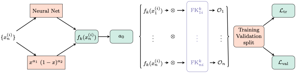
Figure 7: Structure of the NNPDF architecture. Figure slightly modified from Ref. [12].

However, the network architecture is not what makes the NNPDF approach unique in modern machine learning. The second aspects that makes network parton densities special is that they are distributions, similar to but not quite probability distributions, which means they are only defined stochastically. Even for arbitrarily precise data $\sigma$ and predictions $\hat{\sigma}_{ij}$, the best-fit parton densities will fluctuate the same way that solutions of incomplete inverse problems will fluctuate. The NNPDF approach distinguishes between three sources of uncertainty in this situation:

1. even ignoring uncertainties on the data, we cannot expect that the unique minimum in data space translates into a unique minimum in the space of of parton densities. This means the extracted parton densities will fluctuate between equally good descriptions the training data;

2. once we introduce an uncertainty on the data, we can fix the mean values in the data distribution to the truth and introduce an uncertainty through the toy datasets. Now the the minimum in data space is smeared around the true value above, adding to the uncertainty in PDF space;

3. finally, the data is not actually distributed around the truth, but it is stochastic. This again adds to the uncertainties and it adds noise to the set of extracted parton densities.

In the categorization of uncertainties in Sec. 1.2.5 we can think of the first uncertainty as an extreme case of model uncertainty, in the sense that the network is so expressive that the available training data does not provide a unique solution. This problem might be alleviated when adding more precise training data, but it does not have to. This is a standard problem in defining and solving inverse problems, as we will discuss in Sec. 5. The second uncertainty is statistical in the sense that it would vanish in the limit of an infinitely large training dataset. The third uncertainty is the stochastic uncertainty introduced before, again not vanishing for larger training datasets.

Another problem of how to account for all these uncertainties in the extracted parton densities is that they require a forward simulation, followed by a comparison of generated kinematic distributions to data. The solution applied by NNPDF is to replace the dataset and its uncertainties by a sample of data replicas, with a distribution which reproduces the actual data, in the Gaussian limit the mean and the standard deviation for each data point. Each of these toy datasets is then used to train a NNPDF parton density, and the analysis of the parton densities, for instance their correlations and uncertainties, can be performed based on this set of non-parametric NNPDFs. The same method is applied to other global analyses at the LHC, typically when uncertainties or measurements are correlated and likelihood distributions are not Gaussian. A way to check the uncertainty treatment is to validate it starting from a known set of pseudo-data and apply closure tests.

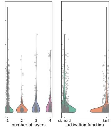
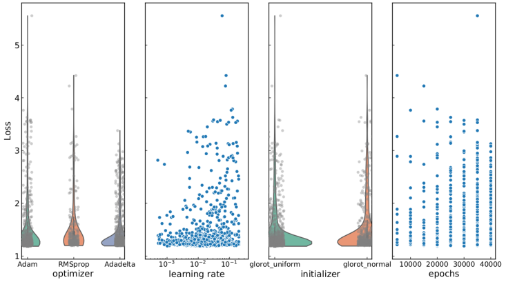
Figure 8: Hyperparameter scan for a test of the NNPDF stability, based on data from photon–proton and electron–proton scattering only. The $y$-axis shows the average of the test and validations losses. Figure from Ref. [13].

As the final step of accounting for uncertainties, NNPDF systematically tests for unwanted systematic biases through the choice of network architecture and hyperparameters. For a precision non-parametric fit, where the implicit bias or the smooth interpolation properties of a network play the key role, it is crucial that the network parameters do induce an uncontrolled bias. For instance, a generic $x$-resolution determined by the network hyper-parameters could allow the network to ignore certain features and overtrain on others. In Fig. 8 we see the dependence of the network performance on some network parameters tested in the NNPDF scan. Each panel shows the loss as a function of the respective network parameter for 2000 toy densities, specifically the average of the test and validation losses. These figures are based on a fit only to data from single-proton interactions with electrons or (virtual) photons. The violin shape is a visualization of the density of points as a function of the loss. The different shapes show how the network details have a sizeable effect on the network performance.

The final NNPDF network architecture and parameters are determined through an automatic hyperoptimization. Because the training and validation datasets are already used in the network training shown in Fig. 7, the hyperoptimization requires another dataset. At the same time, we do not want to exclude relevant data from the final determination of the parton densities, and the result of the hyperoptimization will also depend on the dataset used. The best way out is to use $k$-folding to generate these datasets. Here we divide the dataset into $n_{\text{fold}}$ partitions, and for each training we remove one of the folds. The final loss for each hyperparameter value is then given by the combination of the losses of the $n_{\text{fold}}$ individual trainings,

$$\mathcal{L}_{\text{hyperopt}}=\frac{1}{n_{\text{fold}}}\sum_{k}\mathcal{L}_{k}\;,$$ (1.74)

where the individual losses are given above. Using the sum of the individual losses turns out to be equivalent to using the maximum of the individual losses.

An especially interesting question to ask is what progress we have made in understanding parton densities over the last decade, both from a data perspective and based on the generalized fit methodology. The density to use for this study is the gluon density, because its growth at small $x$-values is poorly controlled by theory arguments and assumed fit functions, which means our description of $f_{g}(x\ll 1)$ is driven by data and an unbiased interpretation of the data. In Fig. 9 we show this gluon density for three different datasets: (i) pre-HERA data consists or fixed-target or beam-on-target measurements of two kinds, photon–proton or electron–proton, and proton-proton interactions; (ii) Pre-LHC data adds HERA measurements of electron–proton scattering at small $x$-values and Tevatron measurements of weak boson production in proton–antiproton scattering; (iii) NNPDF data then adds a large range of LHC measurements. The difference between the NNPDF3.1 and NNPDF4.0 datasets is largely the precision on similar kinematic distributions.

In the two panels of Fig. 9 we first see that the NNPDF3.1 and NNPDF4.0 descriptions of pre-HERA data give an unstable gluon density for $x<10^{-2}$, where this dataset is simply lacking information. The gluon density in this regime is largely an extrapolation, and we already know that neural networks are interpolation tools and not particularly good at magic or extrapolation. From an LHC physics perspective, very small $x$-values are not very relevant, because we can estimate the minimum typical $x$-range for interesting central processes as

$$x_{1}x_{2}\sim\frac{m_{W,Z,H}^{2}}{(14~{}\text{TeV})^{2}}\sim\frac{1}{140^{2}}\qquad\Leftrightarrow\qquad x_{1}\sim x_{2}\sim 7\cdot 10^{-3}\;.$$ (1.75)

Adding HERA data constrains this phase space region down to $x\sim 10^{-3}$ and pushes the central value of the gluon density to a reasonable description. Finally, adding LHC data only has mild effects on the low-$x$ regime, but makes a big difference around $x>0.05$, where we measure the top Yukawa coupling in $t\bar{t}H$ production or test higher-dimensional operators in boosted $t\bar{t}$ production. Comparing the left and right panels of Fig. 9 shows that the new NNPDF methodology leads to extremely small uncertainties for the gluon density for the entire range $x=10^{-2}~{}...~{}1$, where a large number of LHC processes with their complex correlations make the biggest difference. The quoted uncertainties account for the historic increase of the dataset faithfully, except for the pre-HERA guess work.

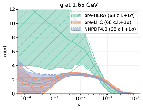
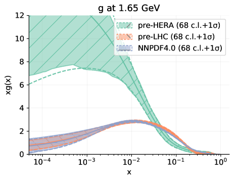
Figure 9: Historic pre-HERA and pre-LHC gluon densities with the NNPDF3.1 (left) and the NNPDF4.0 methodologies, compared with the full respective datasets of the two methodologies. Ref. [12].

2 Classification

After the short introduction to the simpler regression networks, we come back to classification as the standard problem in LHC physics. Whenever we look at a jet or an event, the first question will be what kind of particles gave us that final state configuration. This is not trivial, given that jets are complex objects which can come from a light quark or a gluon, but also from quarks that decay through the electroweak interaction at the hadron level, like charm or bottom quarks. They can also come from a tau lepton, decaying to quarks and a neutrino, or from boosted gauge bosons or Higgs bosons or top quarks. Even when we are looking for apparently simple electrons, we need to be sure that they are not one of the many charged pions which can look like electrons especially in the forward detector. Similarly, photons are not trivial to separate from neutral pions when looking at the electromagnetic calorimeter. Really, the only particle which we can identify fairly reliably at the LHC are muons.

At the event level we ask the same question again, usually in the simple form signal vs background. As an example, we want to extract $t\bar{t}H$ events with an assumed decay $H\to b\bar{b}$, as mentioned in Eq.(1.3), from a sample which is dominated by the $t\bar{t}b\bar{b}$ continuum background and $t\bar{t}jj$ events where we mis-tagged a light-flavor quark or gluon jet as a $b$-quark. Once we have identified $t\bar{t}H$ events we can use them to measure for example the value of the top Yukawa coupling or see if this coupling respects the CP-symmetry or comes with a complex phase. All of this is classification, and from our experience with BDTs for jet and event classification, it is clear that modern neural networks can improve their performance. Of course, the really interesting part is where we turn our expertize in these standard classification task into new ideas, methods, or tools. So the first ML-chapter of these lecture notes will be on classification with modern neural networks.

We have already introduced many of the underlying concepts and technical terms for classification tasks for BDTs in Sec. 1.2.1, especially the fact that we need to minimize the sampled log-likelihood ratio of the data and model densities as described in Eqs.(1.10) and (1.12). We also know from Sec. 1.2.4 that the key ingredient to any neural network and its training is the loss function. We can now put these two things together, implying that for NN-classification we want to learn a signal and a background distribution by minimizing two KL-divergences through our likelihood-ratio loss

$$\mathcal{L}_{\text{class}} =\sum_{j=S,B}D_{\text{KL}}[p_{\text{data},j},p_{\text{model},j}]$$

$$=\Big{\langle}\log p_{\text{data},S}-\log p_{\text{model},S}\Big{\rangle}_{p_{\text{data},S}}+\Big{\langle}\log p_{\text{data},B}-\log p_{\text{model},B}\Big{\rangle}_{p_{\text{data},B}}$$

$$=-\Big{\langle}\log p_{\text{model},S}\Big{\rangle}_{p_{\text{data},S}}-\Big{\langle}\log p_{\text{model},B}\Big{\rangle}_{p_{\text{data},B}}+\text{const}(\theta)$$

$$\Rightarrow\qquad \boxed{\mathcal{L}_{\text{class}}=-\sum_{\{x\}}\;\Big{[}p_{\text{data},S}\log p_{\text{model},S}+p_{\text{data},B}\log p_{\text{model},B}\Big{]}}\;.$$ (2.1)

We consistently omit the arguments $x$ and $\theta$ which we included in Sec. 1.2.1. If we take into account that every jet or event has to either signal or background, $p_{S}+p_{B}=1$, this is just the cross entropy given in Eq.(1.15), but derived as a likelihood loss for classification networks. Looking back at Eq.(1.11) this simple form of the classification loss tells us that we made the right choice of KL-divergence.

To mimic the training procedure, we can do variation calculus to describe the minimization of the loss with respect to $\theta$,

$$\theta_{\text{trained}}=\text{argmin}_{\theta}\mathcal{L}_{\text{class}}=\text{argmin}_{\theta}\sum_{j=S,B}D_{\text{KL}}[p_{\text{data},j}(x),p_{\text{model},j}(x|\theta)]\;.$$ (2.2)

We then replace $p_{B}=1-p_{S}$ and do a variation with respect to the $\theta$-dependent model distribution

$$0 \stackrel{{\scriptstyle!}}{{=}}-\frac{\delta}{\delta p_{\text{model},S}}\sum_{\{x\}}\;\Big{[}p_{\text{data},S}\log p_{\text{model},S}+(1-p_{\text{data},S})\log(1-p_{\text{model},S})\Big{]}$$

$$=-\sum_{\{x\}}\;\Bigg{[}\frac{p_{\text{data},S}}{p_{\text{model},S}}-\frac{1-p_{\text{data},S}}{1-p_{\text{model},S}}\Bigg{]}\qquad\qquad\Leftrightarrow\qquad\qquad\boxed{p_{\text{data},S}=p_{\text{model},S}}$$ (2.3)

If we work under the assumption that a loss function should be some kind of log-probability or log-likelihood, we can ask if our minimized loss function corresponds to some kind of statistical distribution. Again using $p_{B}=1-p_{S}$ as the only input in addition to the definition of Eq.(2.1) we find

$$\mathcal{L}_{\text{class}} =-\sum_{\{x\}}\;\Big{[}p_{\text{data},S}\log p_{\text{model},S}+(1-p_{\text{data},S})\log(1-p_{\text{model},S})\Big{]}$$

$$=-\sum_{\{x\}}\;\log\Big{[}p_{\text{model},S}^{p_{\text{data},S}}\;(1-p_{\text{model},S})^{1-p_{\text{data},S}}\Big{]}\;.$$ (2.4)

We can compare the term in the brackets with the Bernoulli distribution in Eq.(1.50), which gives the probability distributions for two discrete outcomes. We find that an interpretation in terms of the Bernoulli distribution requires for the outcomes and the expectation value

$$p_{\text{data},S}=x\in\{0,1\}\qquad\text{and}\qquad p_{\text{model},S}=\rho$$ (2.5)

This means that our learned probability distribution has a Bernoulli form and works on signal or background jets and events, encoding the signal vs background expectation value encoded in the trained model.

If we follow this line of argument, our classification network should encode and return a signal probability for a given jet or event, which means the final network layer has to ensure that the network output is $f_{\theta}(x)\in[0,1]$. For usual networks this is not the case, but we can easily enforce this by replacing the ReLU activation function in the network output layer with a sigmoid function,

$$\text{Sigmoid}(x)=\frac{1}{1+e^{-x}}\qquad\Leftrightarrow\qquad\text{Sigmoid}^{-1}(x)\equiv\text{Logit}(x)=\log\frac{x}{1-x}\;.$$ (2.6)

The activation function(s) inside the network only work as a source of non-linearity and can be considered just another hyper-parameter of the network. The sigmoid guarantees that the output of the classification network is automatically constrained to a closed interval, so it can be interpreted as a probability without the network having to learn this property. With the loss function of Eq.(2.1) and the sigmoid activation of Eq.(2.6) we are ready to tackle classification tasks.

The final set of naming conventions we need to introduce is the structure of the training data, for example for classification. If we train a network to distinguish, for instance, light-flavor QCD jets from boosted top quarks, the best training data should be jets for which we know the truth labels. In LHC physics we can produce such datasets using precision simulations, including full detector simulations. We call network training on fully labeled data (fully) supervised learning. The problem with supervised learning at the LHC is that it has to involve Monte Carlo simulations. We will discuss below how we can define dominantly top jet samples. However, no sample is ever 100% pure. This means that training on LHC data will at best start from a relatively pure signal and background samples, for which we also know the composition from simulations and a corresponding analysis. Training a classifier on samples with known signal and background fractions is called weakly supervised learning, and whenever we talk about supervised learning on LHC data we probably mean weakly supervised learning with almost pure samples. An interesting question is how we would optimize a network training between purity and statistics of the training data. Of course, we can find compromises, for instance training a network on a combination of labeled and unlabeled data. This trick is called semi-supervised learning and can increase the training statistics, but there seems to be no good example where this helps at the LHC. One of the reasons might be that training statistics is usually not a problem in LHC applications. Finally, we can train a network without any knowledge about the labels, as we will see towards the end of this section. Here the questions we can ask are different from the usual classification, and we refer to this as unsupervised learning. This category is exciting, because it goes beyond the usual LHC analyses, which tend to be based on likelihood methods, hypothesis testing, and applications of the Neyman-Pearson lemma. Playing with unsupervised learning is the ultimate test of how well we understand a dataset, and we will discuss some promising methods in Sec. 3.

2.1 Convolutional networks

Modern machine learning, or deep learning, has become a standard numerical method in essentially all aspects of life and research. Two applications dominate the applications of modern networks, image recognition and natural language recognition. It turns out that particle physics benefits mostly from image recognition research. The most active field applying such image-based methods is subjet physics. It has, for a while, been a driving field for creative physics and analysis ideas at the LHC. An established subjet physics task like identifying the parton leading to an observed jet, is ideal to develop ML-methods to beat standard methods. The classic, multivariate approach has two weaknesses. First, it only uses information preprocessed into theory-inspired and high-level observables. This can be cured in part by using the more low-level observables shown in Eq.(1.6). However, when we just pile up observables we need to ask how well a BDT can capture the correlations. Altogether we need to ask the question is we cannot systematically exploit low-level information about a jet to identify its partonic nature.

2.1.1 Jet images and top tagging

A standard benchmark for jet classification is to separate boosted, hadronically decaying top quarks from QCD jets. Tops are the only quarks which decay through their electroweak interactions before can form hadrons,

$$t\to bW^{+}\to b\ell^{+}\nu_{\ell}\qquad\text{or}\qquad t\to bW^{+}\to bu\bar{d}\;.$$ (2.7)

Most top quarks are produced in pairs and at low transverse momentum. However, even in the Standard Model a fraction of top quarks will be produced at large energies. For heavy resonances, like a new $Z^{\prime}$ gauge boson decaying to top quarks, the tops will receive transverse momenta around

$$p_{T,t}\sim p_{T,\bar{t}}\sim\frac{m_{Z^{\prime}}}{2}-m_{t}\;.$$ (2.8)

For a 2-prong jet we can compute the typical angular separation between the two decay jets as a function of the mass and the transverse momentum, for example in case of a hadronic Higgs decay

$$R_{b\bar{b}}\approx\frac{1}{\sqrt{z(1-z)}}\;\frac{m_{H}}{p_{T,H}}>\frac{2m_{H}}{p_{T,H}}\;.$$ (2.9)

The parameter $z$ describes how the energy is divided between the two decay subjets. Because $R$ is a purely angular separation, it can become large if one of the two decay products becomes soft. A single decay jet is most collimated if the energy is split evenly between the two decay products, which is also the most likely outcome for most decays. For a 3-prong decay like the top quark we leave it at an order-of-magnitude estimate of a fat top jet,

$$R_{bjj}\gtrsim\frac{m_{t}}{p_{T,t}}\;.$$ (2.10)

The inverse dependence can easily be seen when we simulate top decays. For a standard jet size of $R\sim 0.8$ this relation means we can tag top jets for $p_{T,t}\gtrsim 300$ GeV, corresponding to decaying resonances with $m_{Z^{\prime}}>1$ TeV. Given the typical reach of the LHC in resonance searches, this value of $m_{Z^{\prime}}$ as introduced in Eq.(2.8) is actually small, which means that many resonance searches with hadronic decays nowadays rely on boosted final states and fat jets from heavy particle decays.

Before we go into the details of ML-based jet tagging we need to briefly introduce the standard method to define and analyze jets. Acting on calorimeter output in the usual $\Delta\eta$ vs $\Delta\phi$ plane, we usually employ QCD-based algorithms to determine the partonic origin of a given configuration. Such jet algorithms link physical objects, for instance calorimeter towers or particle flow objects, to more or less physical objects, namely partons from the hard process. In that sense, jet algorithms invert the statistical forward processes of QCD splittings, hadronization, and hadron decays, shown in Fig. 2. Recombination algorithms try to identify soft or collinear partners amongst the jet constituents, because we know from QCD that parton splitting are dominantly soft or collinear. We postpone a more detailed discussion to Secs. 3.1 and 5.2.2 and instead just mention that in the collinear limit we can describe QCD splittings again in terms of the energy fraction $z$ of the outgoing hard parton. For example, a quark radiates a gluon following the splitting pattern

$$\hat{P}_{q\leftarrow q}(z)\propto\frac{1+z^{2}}{1-z}\;.$$ (2.11)

To decide if two subjets come from one parton leaving the hard process we have to define a geometric measure capturing the collinear and soft splitting patterns. Such a measure should include the distance $R_{ij}$ defined in Eq.(1.2) and the transverse momentum of one subjet with respect to another or to the beam axis. The three standard measures are

$$k_{T}\qquad\qquad y_{ij} =\frac{R_{ij}}{R}\;\min\left(p_{T,i},p_{T,j}\right)\qquad\qquad\qquad y_{iB} =p_{T,i}$$

C/A $$y_{ij} =\frac{R_{ij}}{R} y_{iB} =1$$

$$\text{anti-}k_{T} y_{ij} =\frac{R_{ij}}{R}\min\left(p_{T,i}^{-1},p_{T,j}^{-1}\right) y_{iB} =p_{T,i}^{-1}\;.$$ (2.12)

The parameter $R$ only balances competing jet–jet and jet–beam distances. In an exclusive jet algorithm we define two subjets as coming from one jet if $y_{ij}<y_{\text{cut}}$, where $y_{\text{cut}}$ is an input resolution parameter. The jet algorithm then consists of the steps

• (1) for all combinations of two subjets find $y^{\text{min}}=\text{min}_{ij}(y_{ij},y_{iB})$

• (2a) if $y^{\text{min}}=y_{ij}<y_{\text{cut}}$ merge subjets $i$ and $j$ and their momenta, keep only the new subjet $i$, go back to (1)

• (2b) if $y^{\text{min}}=y_{iB}<y_{\text{cut}}$ remove subjet $i$, call it beam radiation, go back to (1)

• (2c) if $y^{\text{min}}>y_{\text{cut}}$ keep all subjets, call them jets, done

Alternatively, we can give the algorithm the minimum number of physical jets and stop there. As determined by their power dependence on the transverse momenta in Eq.(2.12), three standard algorithms start with soft constituents ($k_{T}$), purely geometric (Cambridge–Aachen), or hard constituents (anti-$k_{T}$) to form a jet. While for the $k_{T}$ and the $C/A$ algorithms the clustering history has a physical interpretation and can be associated with some kind of time, it is not clear what the clustering for the anti-$k_{T}$ algorithm means.

Once we understand the clustering history of a jet, we can try to determine its partonic content. At this point we are most interested in finding out if we are looking at the decay jet of a massive particle or at a regular QCD jets. For this purpose we start with the observables given in Eq.(1.6). For massive decays we can supplement this set by dedicated tagging observables. For instance, we construct a proper measure for the number of prongs in a jet in terms of the $N$-subjettiness variables

$$\tau_{N}=\frac{1}{R\sum_{k}p_{T,k}}\sum_{k}p_{T,k}\;\min\left(R_{1,k},R_{2,k},\cdots,R_{N,k}\right)^{\beta}\;.$$ (2.13)

It starts with $N$ so-called $k_{T}$-axes, and a reference distance $R$ combined with a typical power $\beta=1$, and matches the jet constituents to a given number of axes. A small value $\tau_{N}$ indicates consistency with $N$ or less substructure axes, so an $N$-prong decay returns a small ratio $\tau_{N}/\tau_{N-1}$, like $\tau_{2}/\tau_{1}$ for $W$-boson or Higgs tagging, or $\tau_{3}/\tau_{2}$ for top tagging. To identify boosted heavy particles decaying hadronically we we can also use a mass drop in the jet clustering history,

$$\max(m_{1},m_{2})<0.8\;m_{1+2}\;.$$ (2.14)

If we approximate the full kinematics in the transverse plane, we can replace the mass drop with a drop in transverse momentum, such that we search for electroweak decays by requiring $\min(p_{T1},p_{T2})>p_{T1+2}$. We can improve the tagging by correlating the two conditions, on the one hand an enhanced $p_{T}$-drop and on the other hand two decay subjets boosted together. This defines the SoftDrop criterion,

$$\frac{\min(p_{T1},p_{T2})}{p_{T1}+p_{T2}}>0.2\left(\frac{R_{12}}{R}\right)^{\beta}\;,$$ (2.15)

for instance with $\beta=1$. It allows us to identify decays through the correlation given in Eq.(2.9). All of these theory-inspired observables, and more, can be applied to jets and define multivariate subjet analysis tools. Here we typically use the boosted decision trees introduced in Sec. 1.2.1. The question is how modern neutral networks, like CNNs, working on jet representations like the jet images of Fig. 10, will perform on such an established jet tagging task.

There are a few reasons why top tagging has become the Hello World of classic or ML-based subjet physics. First, as discussed above, the distinguishing features or top jets are theoretically well defined. Top decays are described by perturbative QCD, and the corresponding mass drop and 3-prong structure can be defined in a theoretically consistent manner without issues with a soft and collinear QCD description. Second, top tagging is a comparably easy task, given that we can search two mass drops, three prongs, and an additional $b$-tag within the top jet. Third, in Sec. 2 we mentioned that it is possible to define fairly pure top-jet samples using the boosted production process

$$pp\to t\bar{t}\to(bu\bar{d})\;(\bar{b}\ell^{-}\bar{\nu})\qquad\text{with}\qquad p_{T,t}\sim p_{T,\bar{t}}\gtrsim 500~{}\text{GeV}\;.$$ (2.16)

We trigger on the hard and isolated lepton, reconstruct the leptonically decaying top using the $W$-mass constraint to replace the unknown longitudinal momentum of the neutrino, and then work with the hadronic recoil jet to, for instance, train or calibrate a classification network on essentially pure samples.

The idea of an image-based top tagger is simple — if we look at the ATLAS or CMS calorimeters from the interaction point, they look like the shell of a barrel, which can be unwrapped into a 2-dimensional plane with the coordinates rapidity $\eta\approx-4.5~{}...~{}4.5$ and azimuthal angle $\phi=0~{}...~{}2\pi$, with the distance measure $R$ defined in Eq.(1.2). If we encode the transverse energy deposition in the calorimeter cells as color or grey-scale images, we can use standard image-recognition techniques to study jets or events. The network architecture behind the success of ML-image analyses are convolutional networks, and their application to LHC jet images started with Ref. [14]. We show a set of average jet images for QCD jets and boosted top decays in Fig. 10. The image resolution of, in this case $40\times 40$ pixels is given by the calorimeter resolution of $0.04\times 2.25^{\circ}$ in rapidity vs azimuthal angle. A single jet image looks nothing like these average images. For a single jet image, only 20 to 50 of the 1600 pixels have sizeable $p_{T}$-entries, making even jet images sparse at the 1% or 2% level, not even talking about full event images. Nevertheless, we will see that standard network architectures outperform all established methods used in subjet physics.

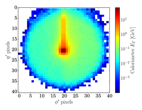
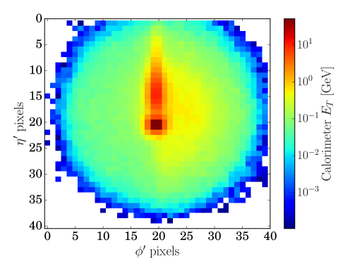
Figure 10: Averaged and preprocessed jet images for a QCD jet (left) and a boosted top decay (right) in the rapidity vs azimuthal plane plane. The preprocessing steps are introduced in the next section. Figures from Ref. [15].

2.1.2 Architecture

The basic idea of convolutional networks is to provide correlations between neighboring pixels, rather than asking the network to learn that pixels 1 and 41 of a jet image lie next to each other. In addition, learning every image pixel independently would require a vast number of network parameters, which typically do not correspond to the actual content of an image. Alternatively, we can try to learn structures and patterns in an image under the assumption that a relatively small number of such patterns encode the information in the image. In the simplest case we assume that image features are translation-invariant and define a learnable matrix-like filter which applies a convolution and replaces every image pixel with a modified pixel which encodes information about the 2-dimensional neighborhood. This filter is trained on the entire image, which means that it will extract the nature and typical distance of 2-dimensional features. To allow for some self-similarity we can then reduce the resolution of the image pixels and run filters with a different length scale. A sizeable number of network parameters is then generated through so-called feature maps, where we run several filters over the same image. Of course, this works best if the image is not sparse and translation-invariant. For example, an image with diagonal features will lead to a filter which reflects the diagonal structure.

In Fig. 11 we illustrate a simple architecture of a convolutional network (CNN) applied to classify calorimeter images of LHC jets. The network input is the 2-dimensional jet image, $(n\times n)$-dimensional matrix-valued inputs $x$ just like in Eq.(1.26), and illustrated in Fig. 10. It then uses a set of standard operations:

• Zero padding $(n\times n)\to(n+1\times n+1)$: It artificially increases the image size by adding zeros to be able to use a filter for the pixels on the boundaries

  $$x_{ij}\;\to\;\begin{pmatrix}0&\cdots&0\\ \vdots&x_{ij}&\vdots\\ 0&\cdots&0\end{pmatrix}\;.$$ (2.17)

• Convolution $(n\times n)\to(n\times n)$: To account for locality of the images in more than one dimension and to limit the number of network parameters, we convolute an input image with a learnable filter of size $n_{\text{c-size}}\cdot n_{\text{c-size}}$. These filters play the role of the nodes in Eq.(1.28),

  $$\boxed{x^{\prime}_{ij}=\sum_{r,s}W_{rs}\;x_{i+r,j+s}+b\to\text{ReLU}(x^{\prime}_{ij})}\;.$$ (2.18)

  As for any network we also apply a non-linear element, for example the ReLU activation function defined in Eq.(1.29).

• Feature maps $n_{\text{f-maps}}\times(n\times n)\to n_{\text{f-maps}}\times(n\times n)$: Because a single learned filter for each convolutional layer defines a small number of network parameters and may also be unreliable in capturing the features correctly, we introduce a set of filters which turn an image into $n_{\text{f-maps}}$ feature maps. The convolutional layer now returns a feature map $x^{\prime(k)}$ which mixes information from all input maps

  $$x^{\prime(k)}_{ij}=\sum_{l=0}^{n_{\text{f-maps}}-1}\quad\sum_{r,s}W^{(kl)}_{rs}\;x^{(l)}_{i+r,j+s}+b^{(k)}\qquad\text{for}\quad k=0,...,n_{\text{f-maps}}-1\;.$$ (2.19)

  Zero padding and convolutions of a number of feature maps define a convolutional layer. We stack $n_{\text{c-layer}}$ of them. Each $n_{\text{c-block}}$ block keeps the size of the feature maps, unless we use the convolutional layer to slowly reduce their size.

  

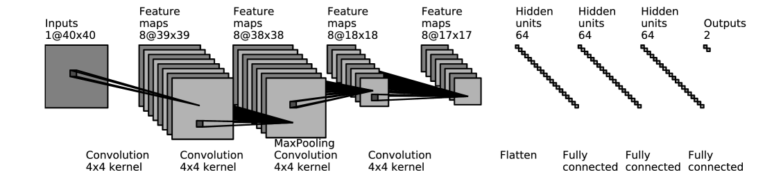
  Figure 11: Simple CNN architecture for the analysis of jet images. Figure from Ref. [15], for a more competitive version see Ref. [16].

• Pooling $(n\times n)\to(n/p\times n/p)$: We can reduce the size of the feature map through a downsampling algorithm. For pooling we divide the input into patches of fixed size $p\times p$ and assign a single value to each patch, for example a maximum or an average value of the pixels. A set of pooling steps reduces the dimension of the 2-dimensional image representation towards a compact network output. An alternative to pooling are stride convolutions, where the center of the moving convolutional filter skips pixels. In Sec. 4.2.6 we will also study the inverse, upsampling direction.

• Flattening $(n\times n)\to(n^{2}\times 1)$: Because the classification task requires, two distinct outputs, we have to assume that the 2-dimensional correlations are learned and transform the pixel matrix into a 1-dimensional vector,

  $$x=\left(x_{11},\dots,x_{1n},\dots,x_{n1},\dots,x_{nn}\right)\;.$$ (2.20)

  This vector can then be transformed into the usual output of the classification network.

• Fully connected layers $n^{2}\to n_{\text{d-node}}$: On the pixel vectors we can use a standard fully connected network as introduced in Eq.(1.26) with weights, biases, and ReLU activation,

  $$x^{\prime}_{i}=\text{ReLU}\left[\sum_{j=0}^{n^{2}-1}W_{ij}x_{j}+b_{i}\right]\;.$$ (2.21)

  The deep network part of our classifier comes as a number of fully connected layers with a decreasing number of nodes per layer. Finally, we use the classification-specific sigmoid activation of Eq.(2.6) in the last layer, providing a 2-dimensional output returning the signal and background probability for a given jet image.

In this CNN structure it is important to remember that the filters are learned globally, so they do not depend on the position of the central pixel. This means the size of the CNN does not scale with the number of pixels in the input image. Second, a CNN with downsampling automatically encodes different resolutions or fields of vision of the filters, so we do not have to tune the filter size to the features we want to extract. One way to increase the expressivity of the network is a larger number of feature maps, where each feature map has access to all feature maps in the previous layer. The number of network parameters then scales like

$$\#_{\text{CNN-parameters}}\sim n_{\text{c-size}}^{2}\times n_{\text{f-maps}}\times n_{\text{c-layer}}\ll n^{2}\;.$$ (2.22)

Of course, CNNs can be defined in any number of dimensions, including a 1-dimensional time series where the features are symmetric under time shifts. For a larger number of dimensions the scaling of Eq.(2.22) becomes more and more favorable.

As always, we can speed up the network training through preprocessing steps. They are based on symmetry properties of the jet images, as we will discuss them in more detail in Sec. 2.3.3. For jet images the preprocessing has already happened in Fig. 10. First, we define a central reference point, for instance the dominant energy deposition or some kind of main axis or center of gravity. Second, we can shift the image such that the main axis is in its center. Third, we use the rotational symmetry of a single jet by rotating the image such that the second prong is at 12 o’clock. Finally, we flip the image to ensure the third maximum is in the right half-plane. This is the preprocessing applied to the averaged jet images shown in Fig. 10. In addition, we can apply the usual preprocessing steps for the pixel entries from Eq.(1.23), plus a unit normalization of the sum of all pixels in an image.

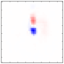
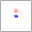
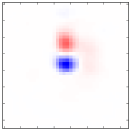
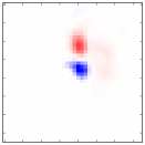
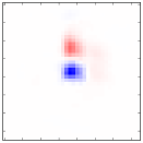
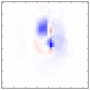
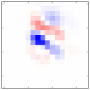
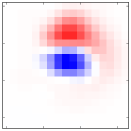
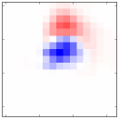
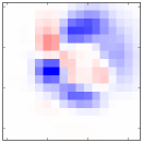
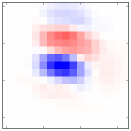
Figure 12: Averaged signal minus background for a simple CNN top tagger. The rows correspond to CNN layers, max-pooling reduces the number of pixels by roughly a factor four. The columns show different feature maps Red areas indicate signal-like regions, blue areas indicate background-like regions. Figure from Ref. [15].

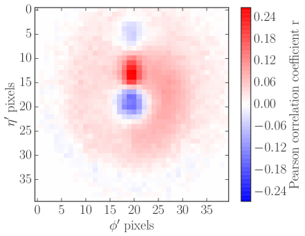
Figure 13: Pearson correlation coefficient for 10,000 signal and background images each. The corresponding jet image is illustrated in figure 10. Red areas indicate signal-like regions, blue areas indicate background-like regions. Figure from Ref. [15].

To these jet images we can apply a standard CNN, as illustrated in Fig. 11. Before we show the performance of a CNN-based top tagger we can gain some intuition for what is happening inside the trained CNN by looking at the output of the different layers in the case of fully preprocessed images. In Fig. 12 we show the difference of the averaged output for 100 signal-like and 100 background-like images. Each row illustrates the output of a convolutional layer. Signal-like red areas are typical for top decays, while blue areas are typical for QCD jets. The feature maps in the first layer consistently capture a well-separated second subjet, and some filters of the later layers also capture a third signal subjet in the right half-plane. While there is no one-to-one correspondence between the location in feature maps of later layers and the pixels in the input image, these feature maps still show that it is possible to see what a CNN learns. One can try a similar analysis for the fully connected network layers, but it turns out that we learn nothing.

To measure the impact of the pixels of the preprocessed jet image impact on the extracted signal vs background label, we can correlate the deviation of a pixel $x_{ij}$ from its mean value $\bar{x}_{ij}$ with the deviation of the signal probability $y$ from its mean value $\bar{y}$. The correlation for a given set of combined signal and background images is given by the Pearson correlation coefficient

$$r_{ij}=\frac{\sum_{\text{images}}\left(x_{ij}-\bar{x}_{ij}\right)\left(y-\bar{y}\right)}{\sqrt{\sum_{\text{images}}\left(x_{ij}-\bar{x}_{ij}\right)^{2}}\sqrt{\sum_{\text{images}}\left(y-\bar{y}\right)^{2}}}\;.$$ (2.23)

Positive values of $r_{ij}$ indicate signal-like pixels. In Fig. 13 we show this correlation coefficient for a simple CNN. A large energy deposition in the center leads to classification as background. A secondary energy deposition at 12 o’clock combined with additional energy in the right half-plane means top signal, consistent with Fig. 10.

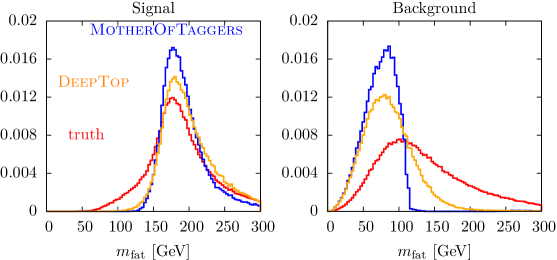
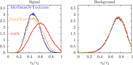
Figure 14: Kinematics observables $m_{\text{fat}}$ and $\tau_{3}/\tau_{2}$ for events correctly determined to be signal or background by the DeepTop CNN and the MotherOfTaggers BDT, as well as Monte Carlo truth. Figure from Ref. [15].

Both, for the CNN and for a traditional BDT tagger we can study signal-like learned patterns in actual signal events by cutting on the output label $y$. Similarly, we can use background-like events to test if the background patterns are learned as expected. In addition, we can compare the kinematic distributions in both cases to the Monte Carlo truth. In Fig. 14 we show the distributions for the fat jet mass $m_{\text{fat}}$ and $\tau_{3}/\tau_{2}$ defined in Eq.(2.13). The CNN and the classic BDT learn essentially the same structures. Their results are even more signal-like than the Monte Carlo truth, because of the stiff cut on $y$. For the CNN and BDT tagger cases this cut removes events where the signal kinematic features is less pronounced. The BDT curves for the signal are more peaked than the CNN curves because these two high-level observables are BDT inputs, while for the neural network they are derived quantities.

Going back to the CNN motivation, it turns our that preprocessed jet images are not translation-invariant, and they are extremely sparse. This means they are completely different from the kind of images CNNs were developed to analyze. While the CNNs work very well for image-based jet classification this raises the question if there are other, better-suited network architectures for jet taggers.

2.1.3 Top tagging benchmark

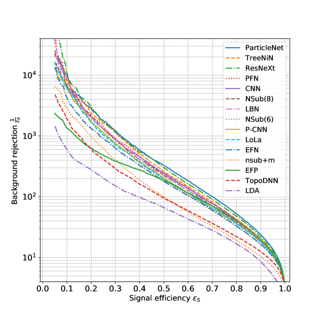
Figure 15: ROC curves for all top-tagging algorithms evaluated on the standard test sample. Figure from Ref. [17].

As common in machine learning, standard datasets are extremely helpful to benchmark the state of the art and develop new ideas. For top tagging, the standard dataset consists of 1M top signal and 1M mixed quark-gluon background jets, produced with the Pythia8 event generator and the simplified detector simulation Delphes. The are divided into 60% training, 20% validation, and 20% test data. The fat jet is defined through the anti-$k_{T}$ algorithm with size $R=0.8$, which means its boundaries in the jet plane are smooth. The dataset only uses the leading jet in each $t\bar{t}$ or di-jet event and requires

$$p_{T,j}=550~{}....~{}650~{}\text{GeV}\qquad\text{and}\qquad|\eta_{j}|<2\;.$$ (2.24)

From Eq.(2.10) we know that we can require a parton-level top and all its decay partons to be within $\Delta R=0.8$ of the jet axis for the signal jets. The jet constituents are extracted through the Delphes energy-flow algorithm, which combines calorimeter objects with tracking output. The dataset includes the 4-momenta of the leading 200 constituents, which can then be represented as images for the CNN application. Particle information is not included, so $b$-tagging cannot be added as part of the top tagging, and any quoted performance should not be considered realistic. The dataset is easily accessible as part of a broader physics-related reference datasets [18].

Two competitive versions of the image-base taggers were benchmarked on this dataset, an updated CNN tagger and the standard ResNeXt network. While the toy CNN shown in Fig. 11 is built out of four successive convolutional layers, with eight feature maps each, and its competitive counterpart comes with four convolutions layers and 64 feature maps, professional CNNs include 50 or 100 convolutional layers. For networks with this depth a stable training becomes increasingly hard with the standard convolutions defined in Eq.(2.19). This issue can be targeted with a residual network, which is built out of convolutional layers combined with skip connections. In the conventions of Eq.(1.27) these skip connections come with the additional term

$$x^{(n-1)}\to x^{(n)}=W^{(n)}x^{(n-1)}+b^{(n)}+x^{\text{(earlier layer)}}\;,$$ (2.25)

where the last term can point to any previous layer. Obviously, we can apply the same structure to the convolutional layer of Eq.(2.18)

$$x^{(n)}_{ij}=\sum_{r,s=0}^{n_{\text{c-size}}-1}W^{(n)}_{rs}\;x^{(n-1)}_{i+r,j+s}+b^{(n)}+x_{ij}^{\text{(earlier layer)}}\;.$$ (2.26)

Again, we suppress the sum over the feature maps. These skip connections are a standard method to improve the training and stability of very deep networks, and we will come across them again.

In Fig. 15 we see that the deep ResNeXt is slightly more powerful than the competitive version of the CNN introduced in Sec. 2.1.2. First, in this study it uses slightly higher resolution with $64\times 64$ pixels. In addition, it is much more complex with 50 layers translating into almost 1.5M parameters, as compared to the 610k parameters of the CNN. Finally, it uses skip connections to train this large number of layers. The sizes of the ResNeXt and the CNN illustrate where some of the power of neural networks are coming from. They can use up to 1.5M network parameters to describe a training dataset consisting of 1M signal and background images each. Each of these sparse calorimeter images includes anything between 20 and 50 interesting active pixels. Depending on the physics question we are asking, the leading 10 pixels might encode most of the information, which translates into 20M training pixels to train 1.5M network parameters. That is quite a complexity, for instance compared to standard fits or boosted decision trees. This complexity also motivates an efficient training, including the back propagation idea, an appropriately chosen loss function, and numerical GPU power. Finally, it explains why some people might be sceptical about the black ox nature of neural networks, bringing us back to the question how we can control what networks learn and assign error bars to their output.

2.1.4 Bayesian CNN

Since we know from Sec. 1.2.4 how to train a network to not only encode some kind of function $f_{\theta}(x)$ but also an uncertainty $\sigma_{\theta}(x)$. We can apply this method to our jet classification task, because it makes a difference if a jet comes with $(60\pm 20)\%$ or $(60\pm 1)\%$ signal probability. Bayesian classification networks provide this information jet by jet. For jet classification this uncertainty could for example come from (i) finite, but perfectly labeled training samples; (ii) uncertainties in the labelling of the training data; and (iii) systematic differences between the training and test samples.

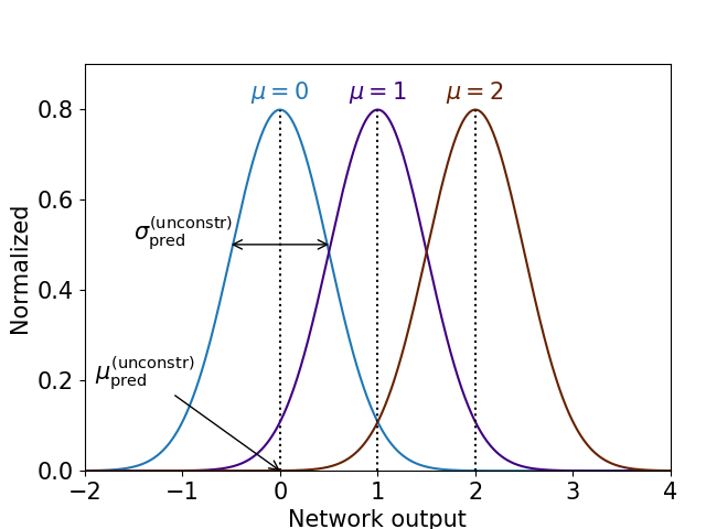
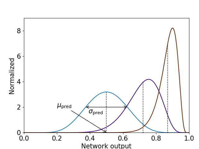
Figure 16: Effect of the sigmoid transformation on Gaussians with the same but different means. Figure from Ref. [19].

The main difference between a regression network and a classification network is that the probability outputs requires us to map unbounded network outputs to the closed interval $[0,1]$ through the final, sigmoid layer given in Eq.(2.6). Such a sigmoid layer will change the assumed Gaussian distribution of the Bayesian network weights. We illustrate this behavior in Fig. 16, where we start from three Gaussians with the same width but different means and apply a sigmoid transformation. The results is that the distributions on the closed interval become asymmetric, to accommodate the fact that even in the tails of the distributions the functional value can never exceed one. The Jacobian of the sigmoid transformation is given by

$$\frac{d\;\text{Sigmoid}(x)}{dx} =\frac{d}{dx}\big{[}1+e^{-x}\big{]}^{-1}=-\frac{1}{\big{[}1+e^{-x}\big{]}^{2}}\frac{d}{dx}\big{[}1+e^{-x}\big{]}=\frac{e^{-x}}{\big{[}1+e^{-x}\big{]}^{2}}$$

$$=\frac{1}{1+e^{-x}}\frac{1+e^{-x}-1}{1+e^{-x}}$$

$$=\text{Sigmoid}(x)\Big{[}1-\text{Sigmoid}(x)\Big{]}\;.$$ (2.27)

We can approximate the standard deviation for example of a Gaussian after the sigmoid transformation assuming a simple linearized form

$$\frac{\sigma_{\text{pred}}^{\text{(sigmoid)}}}{\sigma_{\text{pred}}}\approx\frac{d\sigma_{\text{pred}}^{\text{(sigmoid)}}}{d\sigma_{\text{pred}}}\approx\frac{d\mu_{\text{pred}}^{\text{(sigmoid)}}}{d\mu_{\text{pred}}}=\mu_{\text{pred}}^{\text{(sigmoid)}}\big{[}1-\mu_{\text{pred}}^{\text{(sigmoid)}}\big{]}\;..$$ (2.28)

After the sigmoid transformation the uncorrelated parameters $\mu$ and $\sigma$ turn into a correlated mean and standard deviation; for a transformed mean $\mu_{\text{pred}}^{\text{(sigmoid)}}$ going to zero or one, the corresponding width $\sigma_{\text{pred}}^{\text{(sigmoid)}}$ will vanish. This correlation of the two Bayesian network output is specific to a classification task. This kind of behavior is not new, if we remember how we need to replace the Gaussian by a Poisson distribution, which has the same cutoff feature towards zero count rates.

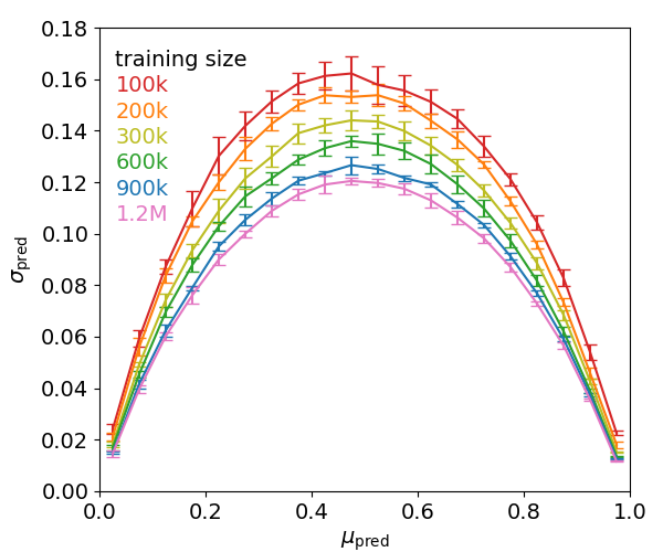
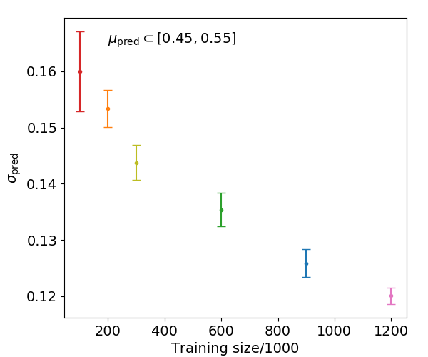
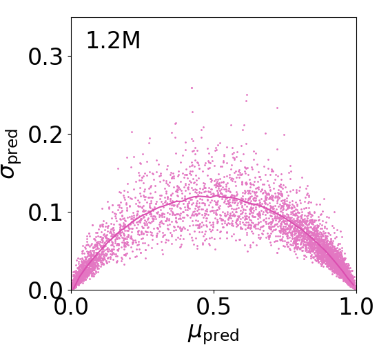
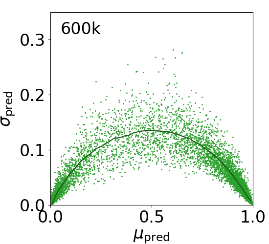
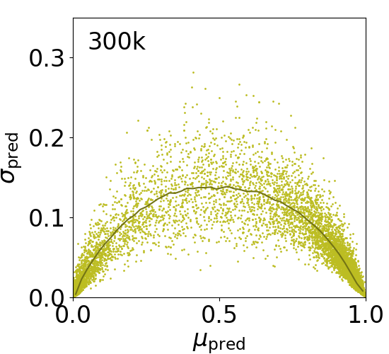
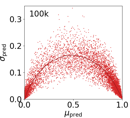
Figure 17: Correlation between predictive mean and standard deviation. The right panel shows the predictive standard deviation for $\mu_{\text{pred}}=0.45~{}...~{}0.55$ as a function of the size of the training sample with the same error bars from different trainings. The lower panels instead show the statistical spread for 10k jets, signal and background combined. Figure from Ref. [19].

To see these correlations we can look at a simple source of statistical uncertainties, a limited number of training jets. In the upper left panel of Fig. 17 we show the correlation between the predictive mean and the predictive standard deviation from the Bayesian CNN. For a single correlation curve we evaluate the network on 10k jets, half signal and half background, and show the mean values of the 10k jets in slices of $\mu_{\text{pred}}$, after confirming that their distributions have the expected Gaussian-like shape. The leading feature is the inverse parabola shape, induced by the sigmoid transform, Eq.(2.28). This is combined with a physics feature, namely that probability outputs around 0.1 or 0.9 correspond to clear cases of signal and background jets, where we expect the predictive standard deviation to be small. In the upper right panel we illustrate the improvement of the network output with an increasing amount of training data for the slice $\mu_{\text{pred}}=0.45~{}...~{}0.55$. The improvement is significant compared to the error bars, which correspond to different training and testing samples. The corresponding spread of these 10k signal and background jets is illustrated in the four lower panels, with a matching color code.

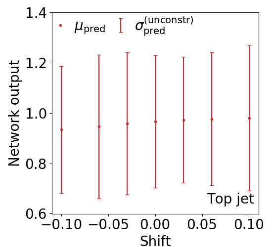
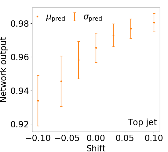
Figure 18: Effect of a shifted energy scale for the hardest constituent on the top tagging, showing the network output before the sigmoid transformation (left) and the classification output (right). Figure from Ref. [19].

One of the great advantages of LHC physics is that we can study the behavior of neural networks on Monte Carlo, before we train or at least use them on data. This also means that we can extend the uncertainty treatment of BNNs to also include systematic uncertainties, as long as we can describe them using data augmentation. An example is the jet or calorimeter energy scale, which is determined through reference measurements and then included in all jet measurements as a function of the detector geometry. Because hard and soft pixels encode different physics information and the calibration of soft pixels is strongly correlated with pile-up removal, we can see what happens for a top tagger when we change the pixel calibration. As a side remark, for this study we do not use the standard CNN, because here the pixel entries are usually normalized. To see an effect on the classification output we shift the energy of the leading jet constituent by up to 10%. In the left panel of Fig. 18 we see that this shift has hardly any effect on the network output before we apply the sigmoid activation. In the right panel we see what happens after the sigmoid activation: depending on the sign of the systematic shift the network is systematically less or more sure that a top jets corresponds to a signal. From a physics perspective this is expected, because top jets are more hierarchical, owed to the weak decays and the mass drop. Changing the calibration of the hard constituent(s) then acts like an adversarial attack on the classification network — a change exactly in the feature that dominates the classification output.

Finally, as mentioned above, using neural networks beyond black-box mode requires to control if the network has captured the underling feature(s) correctly and then assign an error bar to the network output. These two aspects have to be separated, because networks fall into the same trap as people — not knowing anything they tend to underestimate their uncertainty by ignoring unknown unknowns. For Bayesian classification we can tackle this problem: first, we use the correlation of the two outputs $(\mu_{\text{pred}},\sigma_{\text{pred}})$ of the Bayesian classification network for control. A poorly trained network will not reproduce the quadratic correlation of Eq.(2.28) and reveal its fundamental ignorance. Once we have convinced ourselves that the network behaves as expected, we can use the predictive jet-wise uncertainty as an input to the actual analysis.

2.2 Capsules

As we have seen, CNNs are great tools to analyze jet images at the LHC, even though jet images do not look at all like the kind of images these networks were developed for. However, at the LHC we are only interested in jets as an, admittedly extremely interesting, part of a collision event. This leads to the general question is how we can combine information at the event level with the subjet information encoded in each jet. For images this means we move from already sparse jet images to extremely sparse events. For this task, a natural extension of CNNs are capsule networks or CapsNets. They allow us to analyze structures of objects and their geometric layout simultaneously. At the LHC we would like them to combine subjet information with the event-level kinematics of jets and other particles.

The idea of capsules as a generalization of CNNs follows from the observation that CNNs rely on a 1-dimensional scalar representation of images. The idea behind capsules is to represent the entries of the feature maps as vectors in signal or background feature space, depending on which a given capsule describes. Only the absolute value of the capsule encodes the signal vs background classification. The direction of the vectors can track the actual geometric position and orientation of objects, which is useful for images containing multiple different objects. In particle physics, an event image is a perfect example of such a problem, so let us see what we can do when we replaces this single number with vectors extracted from the feature maps.

2.2.1 Architecture

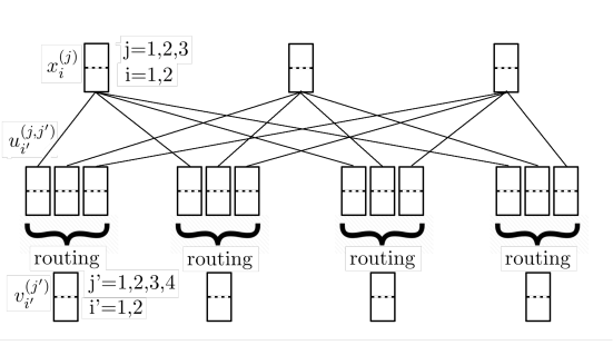
Figure 19: Sketch of a CapsNet module with two simple capsule layers. Figure from Ref. [20].

Just like a scalar CNN, a CapsNet starts with a pixelized image, for instance the calorimeter image of a complete event with $180\times 180$ pixels. It is analyzed with a convolutional filter, combined with pooling or stride convolutions to reduce the size of the feature maps. The CapsNet’s convolutional layers are identical to a scalar CNN. The new idea is to transform the feature maps after the convolution into pixel-wise vectors. Each layer then consists of a number of capsule vectors, for example 24 feature maps with $40\times 40$ entries each can be represented as 1600 capsule-vectors of dimension 24, or 3200 capsules of dimension 12, or 4800 capsules of dimension 8, etc.

The capsules have to transfer information matching their vector property. In Fig. 19 we illustrate a small, 2-layer CapsNet with three initial 2-dimensional capsules $\vec{x}^{(j)}$ linked through routing by agreement to four 2-dimensional capsules $\vec{v}^{(j^{\prime})}$. For deeper networks the dimensionality of the resulting capsule vector can, and should, be larger than the incoming capsule vector. We can write the complete matrix transformation from the input $x$ to the output $v$ as

$$v_{i^{\prime}}^{(j^{\prime})}=\sum_{j=1,2,3}\sum_{i=1,2}\left(C\;W\right)_{i^{\prime}i}^{(j^{\prime}j)}x_{i}^{(j)}\;.$$ (2.29)

The connecting matrix has two sets of indices and size,$2\times 2$ in $i$ and $3\times 4$ in $j$. We can reduce the number of parameters by factorizing the two steps. To get from three to four capsules we first define four combinations of the three initial capsules with the entries $u^{(j,j^{\prime})}_{i^{\prime}}$, related to the initial capsule vectors $\vec{x}^{(j)}$ through trainable weight matrices,

$$u^{(j,j^{\prime})}_{i^{\prime}}=\sum_{i=1,2}W^{(j,j^{\prime})}_{i^{\prime}i}\;x^{(j)}_{i}\qquad\qquad\text{for $j=1,2,3$ and $j^{\prime}=1,2,3,4$}\;.$$ (2.30)

Next, we contract the original index $j$ to define the four outgoing capsules using another set of trainable weights,

$$v_{i^{\prime}}^{(j^{\prime})}=\sum_{j=1,2,3}C^{(j^{\prime},j)}\;u^{(j,j^{\prime})}_{i^{\prime}}\qquad\text{with}\qquad\sum_{j^{\prime}=1,2,3,4}C^{(j,j^{\prime})} =1\quad\forall j\;.$$ (2.31)

The normalization ensures that the contributions from one capsule in the former to each capsule in the current layer add up to one. Furthermore, a squashing step after each capsule layer ensures that the length of every capsule vector remains between 0 and 1,

$$\vec{v}\to\vec{v}^{\prime} =\frac{|\vec{v}|}{\sqrt{1+|\vec{v}|^{2}}}\;\hat{v}\;,$$ (2.32)

with $\hat{v}$ defined as the unit vector in $\vec{v}$-direction.

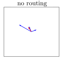
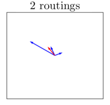
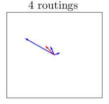
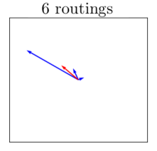
Figure 20: Effects of the routing/squashing combination. In blue we show the intermediate vectors, in red we show the output vector after squashing. Figure from Ref. [20].

Up to now we have constructed a set of four capsules from a set of three capsules through a number of trainable weights, but not enforced any kind of connection between the two sets of capsule vectors. We can extend the transformation in $j$-space, Eq.(2.31), to consecutively align the vectors $\vec{u}^{(j,j^{\prime})}$ and $\vec{v}^{(j^{\prime})}$ through a re-definition of the weights $C^{(j,j^{\prime})}$. This means we compute the scalar product between the vector $\vec{u}^{(j,j^{\prime})}$ and the squashed vector $\vec{v}^{(j^{\prime})}$ and replace in Eq.(2.31)

$$C^{(j,j^{\prime})}\longrightarrow C^{(j,j^{\prime})}+\vec{u}^{(j,j^{\prime})}\cdot\vec{v}^{(j^{\prime})}\;.$$ (2.33)

We can iterate this additional condition and construct a series of vectors $v^{(j^{\prime})}$, which has converged once $\vec{u}^{(j,j^{\prime})}$ and $\vec{v}^{(j^{\prime})}$ are parallel. It is called routing by agreement and is illustrated in Fig. 20, where the blue vectors represent the three $\vec{u}^{(j,j^{\prime})}$ in each set and the red vector is the output $\vec{v}^{(j^{\prime})}$. With each routing iteration the vectors parallel to $\vec{v}^{(j^{\prime})}$ become longer while the others get shorter.

Unlike the CNN, the CapsNet can now encode information in the length and the direction of the output vectors. We typically train the network such that the length of the output vectors provide the classification. Just like for the scalar CNN we differentiate between signal and background images using two output capsules. The more likely the image is to be signal or background, the longer the corresponding capsule vector will be. For simple classification the capsule-specific part of the loss function consists of a 2-terms margin loss

$$\boxed{\mathcal{L}_{\text{CapsNet}}=\max\left(0,m_{+}-|\vec{v}^{(1)}|\right)^{2}+\lambda\max\left(0,|\vec{v}^{(2)}|-m_{-}\right)^{2}}\;.$$ (2.34)

The first term vanishes if the length of the signal vectors $\vec{v}^{(1)}$ exceeds $m_{+}$. The second term vanishes for background vectors $\vec{v}^{(2)}$ shorter than $m_{-}$. Typical target numbers $m_{+}=0.9$ and $m_{-}=0.1$ can sum up to one, nothing forces the actual length of all capsules in a prediction to do the same.

2.2.2 Jets and events

If we want to use CapsNets to analyze full events including subjet information, we can apply them to extract the signal process

$$pp\to Z^{\prime}\to t\bar{t}\to(bjj)\;(\bar{b}jj)$$ (2.35)

with $m_{Z^{\prime}}=1$ TeV from two backgrounds

$$pp\to t\bar{t}\qquad\qquad\text{and}\qquad\qquad pp\to jj\;,$$ (2.36)

all with $p_{T,j}>350$ GeV and $|\eta_{j}|<2.0$. As usual, we transform the calorimeter hits into a 2-dimensional image, now including with $180\times 180$ pixels to covering the entire detector with $|\eta|<2.5$ and $\phi=0~{}...~{}2\pi$.

If we want to extract a signal from two backgrounds we can train the classifier network either on two or on three classes. It often depends on the details of the network architecture and performance what the best choice is. In the case of capsules it turns out that the QCD background rejection benefits from the 3-class setup, because a first capsule can focus on separating the signal from the $t\bar{t}$ continuum background while a dedicated QCD capsule extracts the subjet features. On the other hand, we need to remember is that training multi-class networks require more data to learn all relevant features reliably.

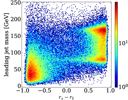
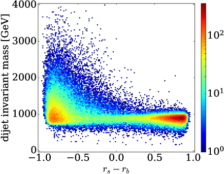
Figure 21: Correlation between capsule outputs $r_{S}-r_{B}$ and the leading jet mass, the di-jet $m_{jj}$, and $\Delta\eta_{jj}$ for true signal and background events. Finally we show the correlation of the signal $\varphi$ vs the the mean $\eta_{j}$ for true signal events. Figure from Ref. [20].

As one advantage of capsules we will see that they can combine jet tagging with event kinematics, a problem for regular CNNs. To simplify our study we train the CapsNet to only separate the $Z^{\prime}(\to t\bar{t})$ signal from QCD di-jet events, so the signal and background differs in event-level kinematics and in jet substructure. We then define a signal-background discriminator

$$r_{S}-r_{B}\equiv|\vec{v}^{(S)}|-|\vec{v}^{(B)}|=\begin{cases}+1&\text{signal events}\\ -1&\text{background events}\end{cases}$$ (2.37)

Confronting this value with two key observables in Fig. 21, we first confirm that the network associates a large jet mass with the top signal, where the secondary peak in the leading jet mass arises from cases where the jet image only includes two of the three top decay jets and learns either $m_{W}$ or the leading $m_{jb}\approx m_{W}$. We also see that the capsules learn to identify the peak in the di-jet invariant mass at approximately 1 TeV as a signal feature, different from the falling spectrum for background-like events.

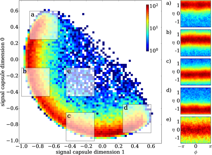
Figure 22: Distribution of the two entries in the 2-dimensional signal capsule for signal events. Right: average event images in the $\eta-\phi$ plane. Figure from Ref. [20].

The second advantage of capsules is that they organize features in their vector structure, so we can understand what the CapsNet has learned. Only a certain combination of the vector entries is required to separate signal and background, the rest of them is free to learn a convenient representation space. This representation can cover patterns which affect the classification output, or not. Again, the two output capsules correspond to the $Z^{\prime}$ signal and the light-flavor QCD background, with two dimensions each, making it easy to visualize the output capsules. The classification output is then mapped back into the image space for visualization purposes.

In Fig. 22 we show the density of the two output entries in the 2-dimensional signal capsule for true signal events. Each event corresponds to a point in the 2-dimensional plane. Because the classification output is proportional to the length of the capsule vector, it corresponds to the distance of each point from the origin. Correctly identified signal events sit on the boundary of the circle segment. The rotation of the circle segment is not fixed a priori, and nothing forces the network to fill the full circle In this 2-dimensional capsule plane we select five representative regions indicated by semi-transparent squares. For each region we identify the contributing events and super-impose their detector images in the $\eta-\phi$ plane in the right panels of Fig. 22. For our signal events we observe bands in rapidity, smeared out in the azimuthal angle. This indicates that the network learns an event-level correlation in the two $\eta_{j}$ as an identifying feature of the signal.

As we can see, the CapsNet architecture is a logical and interesting extension of the CNN, especially when we are interested in combining event-level and jet-level information and in understanding the classification outcome. Capsules define a representation or latent space, which we will come back to in Sec. 2.4. All of this means that CapsNets are extremely interesting conceptually. The problem in particle physics applications is still, that extremely sparse jet or calorimeter images are not the ideal representation, and in Fig. 15 we have seen that other architectures are more promising. So we will leave CapsNets behind, but keep in mind their structural advantages.

2.3 Graphs

In the last section we have argued the case to move from jet images to full event information. Event images work for this purpose, but their increasingly sparse structure cuts into their original motivation. The actual data format behind LHC jets and events are not images, but a set of 4-vectors with additional information on the particle content. These 4-vectors include energy measurements from the calorimeter and momentum measurements from the tracker. The difference between the two is that calorimeters observe neutral and charges particles, while tracking provides information on the charged particles with extremely high angular resolution. Calorimeter and tracking information are combined through dedicated particle flow algorithms, which is probably the better option than combining sparse jet images of vastly different resolution. Now, we could switch from image recognition to natural language recognition networks, but those do not reflect the main symmetry of 4-vectors or other objects describing LHC collisions, the permutation symmetry. Instead, we will see there are image-based concepts which work extremely well with the LHC data format.

2.3.1 4-Vectors and point clouds

The basic constituents entering any LHC analysis are a set of $C$ measured 4-vectors sorted by $p_{T}$, for example organized as the matrix

$$(k_{\mu,i})=\begin{pmatrix}k_{0,1}&k_{0,2}&\cdots\\ k_{1,1}&k_{1,2}&\cdots\\ k_{2,1}&k_{2,2}&\cdots\\ k_{3,1}&k_{3,2}&\cdots\end{pmatrix}\;,$$ (2.38)

where for now we ignore additional information on the particle identification. Such a high-dimensional data representation in a general and often unknown space is called a point cloud. If we assume that all constituents are approximately massless, a typical jet image would encode the relative phase space position to the jet axis and the transverse momentum of the constituent,

$$k_{\mu,i}\quad\to\quad\begin{pmatrix}\Delta\eta_{i}\\ \Delta\phi_{i}\\ p_{T,i}\end{pmatrix}\;.$$ (2.39)

For the generative networks we will introduce in Sec. 4 we implement this transformation as preprocessing, but for the simpler classification network it turns out that we can just work with the 4-vectors given in Eq.(2.38).

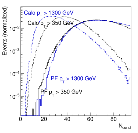
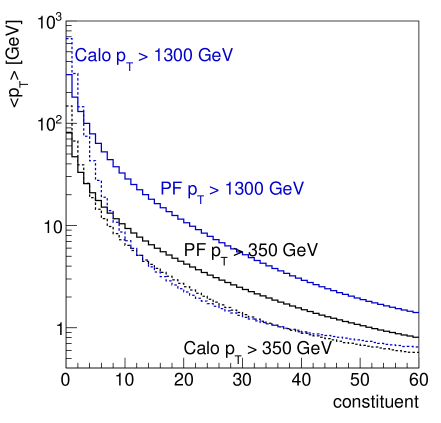
Figure 23: Number of top jet constituents (left) and mean of the transverse momentum (right) of the ranked constituent 4-vectors in Eq.(2.38). We show information from jet images (dashed) and from the combined through particle flow (solid). Figure from Ref. [21].

To illustrate the difference between the image representation and the 4-vector representation we replace our standard top tagging dataset of Eq.(2.24) with two distinct samples, corresponding to moderately boosted tops from Standard Model processes and highly boosted tops from resonance searches,

$$p_{T,j}=350~{}...~{}450~{}\text{GeV}\qquad\text{and}\qquad p_{T,j}=1300~{}...~{}1400~{}\text{GeV}\;.$$ (2.40)

In the left panel of Fig. 23 we show the number of calorimeter-based and particle-flow 4-vectors $k_{\mu,i}$ available for our analysis, $N_{\text{const}}$. We see that including tracking information roughly doubles the number of available 4-vectors and reduces the degradation towards higher boost. In the right panel we show the mean transverse momentum of the $p_{T}$-ordered 4-vectors, indicating that the momentum fraction carried by the charged constituents is sizeable. The fact that the calorimeter-based constituents do not get harder for higher boost indicates a serious limitation from their resolution. In practice, we know that the hardest 40 constituents tend to saturate tagging performances, while the remaining entries will typically be much softer than the top decay products and hence carry little signal or background information from the hard process. Comparing this number to the calorimeter-based on particle flow distributions motivates us to go beyond calorimeter images.

As a starting point, we introduce a simple constituent-based tagger which incorporates some basic physics structure. First, we mimic a jet algorithm and multiply the 4-vectors from Eq.(2.38) with a matrix $C_{ij}$ and return a set of combined 4-vectors $\tilde{k}_{j}$ as linear combinations of the input 4-vectors,

$$k_{\mu,i}\stackrel{{\scriptstyle\text{CoLa}}}{{\longrightarrow}}\widetilde{k}_{\mu,j}=k_{\mu,i}\;C_{ij}\;.$$ (2.41)

The explicit form of the matrix $C$ defining this combination layer (CoLa) ensures that the $\tilde{k}_{j}$ include each original momentum $k_{i}$ as well as a trainable set of $M-C$ linear combinations. These $\tilde{k}_{j}$ could be analyzed by a standard, fully connected or dense network.

However, we already known that the relevant distance measure between two substructure objects, or any two 4-vectors sufficiently far from the closest black hole, is the Minkowski metric. This motivates a Lorentz layer, which transforms the $\tilde{k}_{j}$ into the same number of measurement-motivated invariants $\hat{k}_{j}$,

$$\tilde{k}_{j}\stackrel{{\scriptstyle\text{LoLa}}}{{\longrightarrow}}\hat{k}_{j}=\begin{pmatrix}m^{2}(\tilde{k}_{j})\\ p_{T}(\tilde{k}_{j})\\ \Box_{m}w^{(E)}_{jm}\,E(\tilde{k}_{m})\\ \Box_{m}w^{(d)}_{jm}\,d^{2}_{jm}\\ \end{pmatrix}\;.$$ (2.42)

The first two $\hat{k}_{j}$ map individual $\tilde{k}_{j}$ onto their invariant mass and transverse momentum, using the Minkowski distance between two four-momenta,

$$d^{2}_{jm} =(\tilde{k}_{j}-\tilde{k}_{m})_{\mu}\;g^{\mu\nu}\;(\tilde{k}_{j}-\tilde{k}_{m})_{\nu}\;.$$ (2.43)

In case the invariant masses and transverse momenta are not sufficient to optimize the classification network, the additional weights $w_{jm}$ are trainable. The third entry in Eq.(2.42) constructs a linear combination of all energies, evaluated with one of several possible aggregation functions

$$\Box\in\left\{\text{max},\text{sum},\text{mean},\cdots\right\}\;.$$ (2.44)

Similarly, the fourth entry combines all Minkowski distances of $\tilde{k}_{m}$ with a fixed $\tilde{k}_{j}$. Again, we can sum over or minimize over the internal index $m$ while keeping the external index $j$ fixed.

A technical challenge related to the Minkowski metric for example in a graph convolutional network (GCN) language is that it combines two different features: two subjets are Minkowski-close if they are collinear or when one of them is soft ($k_{i,0}\to 0$). Because these two scenarios correspond to different, but possibly overlapping phase space regions, they are hard to learn for the network. To see how the network does and what kind of structures drive the network output, we turn the problem around and ask the question if the Minkowski metric is really the feature distinguishing top decays and QCD jets. This means we define the invariant mass $m(\tilde{k}_{j})$ and the distance $d_{jm}^{2}$ in Eq.(2.42) with a trainable diagonal metric and find

$$g=\text{diag}( \quad 0.99\pm 0.02,$$

$$-1.01\pm 0.01,-1.01\pm 0.02,-0.99\pm 0.02)\;,$$ (2.45)

where the errors are given by five independently trained copies. This means that for top tagging the appropriate space to relate the 4-vector data of Eq.(2.41) is defined by the Minkowski metric. Obviously, this is not going to be true for all analysis aspects. For instance, at the event level the rapidities or the scattering angles include valuable information on decay products from heavy resonance compared to the continuum background induced by the form of the parton densities. Still, the LoLa tagger motivates the question how we can combine a data representation as 4-vectors with an appropriate metric for these objects.

In Fig. 15 we see that the CoLa-LoLa network does not provide the leading performance. One might speculate that its weakness is that it is a little over-constructed with too much physics bias, with the positive side effect that the network only needs 127k parameters.

The fact that we can extract the Minkowski metric as the relevant metric for top-tagging based on 4-vectors leads us to the concept of graphs. Here we assume that our point-cloud data populates a space for which we can extract some kind of metric or geometry. The optimal metric in this space depends on the task we are training the network to solve. This becomes obvious when we extend the 4-vectors of jet constituents or event objects with entries encoding details from the tracker, like displaced vertices, or particle identification. The question is how we can transform such a point cloud into a structure which allows us to perform the kind of operations we have seen for the CoLa-LoLa tagger, but in an abstract space.

2.3.2 Graph convolutional network

The first problem with the input 4-vectors given in Eq.(2.38) is that we do not know which space they live in. The structure that generalizes our CoLa-LoLa approach to an abstract space is, first of all, based on defining nodes, in our case the vectors describing a jet constituent. These nodes have to be connected in some way, defining an edge between each pair of nodes. The LoLa ansatz in Eq.(2.42) already assumes that these edges have to go beyond the naive Minkowski metric. The object defined by a set of nodes and their edges is called a graph.

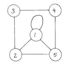
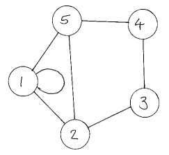
Figure 24: Example for a simple graph.

The basic object for analyzing a graph with $C$ nodes is the $C\times C$ adjacency matrix. It encodes the $C^{2}$ edges, where we allow for self-interactions of nodes. In the simplest case where we are just interested in the question if two nodes actually define a relevant edge, the adjacency matrix includes zeros and ones. In the graph language such an adjacency matrix defines an undirected — edges do not depend on their direction between two nodes — and unweighted. Even for this simple case this matrix can be useful. Let us look at an example of $C=5$ nodes with the six edges

$$A=\begin{pmatrix}2&1&0&0&1\\ 1&0&1&0&1\\ 0&1&0&1&0\\ 0&0&1&0&1\\ 1&1&0&1&0\end{pmatrix}\;.$$ (2.46)

This graph is illustrated in Fig. 24, skipping the 6th node in the image. Because the graph is undirected, the adjacency matrix is symmetric. Only the first node has a self-interaction, which we count twice because it can be used in two directions. Now we can compute powers of the adjacency matrix, like

$$A^{2}=\begin{pmatrix}6&3&1&1&3\\ 3&3&0&2&1\\ 1&0&2&0&2\\ 1&2&0&2&0\\ 3&1&2&0&3\end{pmatrix}\qquad\text{and}\qquad A^{3}=\begin{pmatrix}18&10&4&4&10\\ 10&4&5&1&8\\ 4&5&0&4&1\\ 4&1&4&0&5\\ 10&8&1&5&4\end{pmatrix}\;.$$ (2.47)

The matrix $A^{n}$ encodes the number of different paths of length $n$ which we can take between the two nodes given by the matrix entry. For instance, we can define four length-3 connections between the node and and itself, two different loops each with two directions. Once we have defined a set of edges we can use the existence of an edge, or a non-zero entry in $A$, to define neighboring nodes, and neighboring nodes is what we need for operations like filter convolutions, the basis of a graph-convolutional network.

Once we have defined our set of nodes and their adjacency matrix, the simplest way to use a filter is to go over all nodes and train a universal filter for their respective neighbors. We already know that our nodes are not just a simple number, but a collection of different features. In that case we can define each node with a feature vector $x_{i}^{(k)}$ for the nodes $i=1~{}...~{}C$. In analogy to the feature maps of Eq.(2.19) we can then define a filter $W_{j}^{(kl)}$ where $j$ goes through the neighboring nodes of $i$ and matrix entries match the size of the central and neighboring feature vectors. This means neighboring pixels of Eq.(2.19) become nodes with edges, and feature maps turn into feature vectors. A convolutional network working on one node now returns

$$x^{\prime(k)}_{i}=\sum_{\text{features}\;l}\sum_{\text{neighbors}\;j}W^{(kl)}_{ij}\;x_{j}^{(l)}\equiv\sum_{\text{features}\;l}\sum_{\text{nodes}\;j,j^{\prime}}W^{(kl)}_{ij^{\prime}}A_{j^{\prime}j}\;x_{j}^{(l)}\;,$$ (2.48)

where in the second form we have used the adjacency matrix to define the neighbors. When using such graph convolutions we can add a normalization factor to this adjacency matrix. Obviously, we also need to apply the usual non-linear activation unction, so the network will for instance return $\text{ReLU}(x^{\prime}_{i})$. Finally, for the definition of the universal filter it will matter how we order the neighbors of each node.

Instead of following the convolution explicitly, as in Eq.(2.48), we can define a more general transformation than in Eq.(2.19), namely a vector-valued function of two feature vectors $x_{i,j}$, and with the same number of dimensions as the feature vector $x_{i}$,

$$x^{\prime}_{i}=\sum_{\text{neighbors}\;j}W_{\theta}(x_{i},x_{j})$$ (2.49)

The sum runs over the neighboring nodes, and we omit the explicit sum in feature space. If we consider the strict form of Eq.(2.48) a convolutional prescription, and its extension to $W^{(kl)}_{ij}\to W^{(kl)}_{ij}(x_{i},x_{j})$ as an attention-inspired generalization, the form in Eq.(2.49) is often referred as the most general message passing. Looking at this prescription and comparing it for instance with Eq.(2.42), it is not clear why we should sum over the neighboring nodes, so we can define more generally

$$\boxed{x^{\prime}_{i}=\Box_{j}\;W_{\theta}(x_{i},x_{j})}\;,$$ (2.50)

with the aggregation functions $\Box_{j}$ defined in Eq.(2.44). The corresponding convolutional layer is called an edge convolution. Just like a convolutional filter, the function $W$ is independent of the node position $i$, which means it will scale as economically as the CNN. The form of $W$ allows us to implement symmetries like

$$W_{\theta}(x_{i},x_{j}) =W_{\theta}(x_{i}-x_{j})$$ translation symmetry

$$W_{\theta}(x_{i},x_{j}) =W_{\theta}(|x_{i}-x_{j}|)$$ rotation symmetry

$$W_{\theta}(x_{i},x_{j}) =W_{\theta}(x_{i},x_{i}-x_{j})$$ translation symmetry conditional on center. (2.51)

The most important symmetry for applications in particle physics is the permutation symmetry of the constituents in a jet or the jets in an event. The edge convolution is symmetric as long as $W_{\theta}$ does not spoil such a symmetry and the aggregation function is chosen like in Eq.(2.50).

Going back to the point clouds describing LHC jets or events, we first need to transform the set of possibly extended 4-vectors into a graph with nodes and edges. Obviously, each extended 4-vector of an input jet can become a node described by a feature vector. Edges are defined in terms of an adjacency matrix. We already know that we will modify the adjacency matrix as the initial form of the edges through edge convolutions, so we can just define a reasonably first set of neighbors for each node. We can do that using standard nearest-neighbor algorithms, defining the input to the first edge-convolution layer. When stacking edge convolutions, each layer produces a new set of feature vectors or nodes. This leads to a re-definition of the adjacency matrix after each edge convolution, removing the dependence on the ad-hoc first choice. This architecture is referred to as a Dynamic Graph Convolutional Neural Network (DGCNN). The structure of the edge convolution is shown in the left panel of Fig. 25. It combines the nearest-neighbor definition for the graph input with a series of linear edge convolutions and a skip connection as introduced in Eq.(2.25).

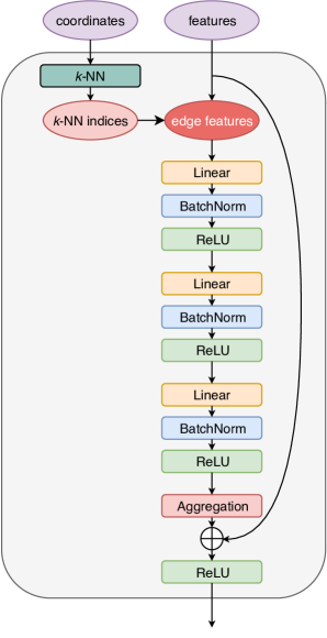
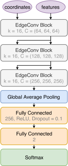
Figure 25: Architectures of an edge convolution block (left) and the ParticleNet implementation for jet tagging. In the right panel, $k$ is the number of nearest neighbors considered and $C$ the number of channels per edge convolution layer. Figure from Ref. [22].

One reason to introduce the dynamic GCN is that it provides the best jet tagging results in Fig. 15. The ParticleNet tagger is based on the third ansatz for the filter function in Eq.(2.51) with the simple linear combination

$$\Box_{j}\;W_{\theta}(x_{i},x_{j})=\text{mean}_{j}\Big{[}\theta_{\text{diff}}\cdot(x_{i}-x_{j})+\theta_{\text{local}}\cdot x_{i}\Big{]}$$ (2.52)

This is the form of the linear convolution referred to in the left panel of Fig. 25. Batch normalization is a way to improve the training of deep networks in practice. It evaluates the inputs to a given network layer for a minibatch defined in Eq.(1.33) and changes their normalization to mean zero and standard deviation one. It is known to improve the network training, even though there seems to be no good physics or other reason for that improvement.

In the right panel of Fig. 25 we show the architecture of the network. After the edge convolutions we need to collect all information in a single vector, which in this case is constructed by average-pooling over all nodes for each of the channels. The softmax activation function of the last layer is the multi-dimensional version of the sigmoid defined in Eq.(2.6), required for a classification network. It defines a vector of the same size as its input, but such that all entries are positive and sum to one,

$$\text{Softmax}_{i}(x)=\frac{e^{x_{i}}}{\sum_{j}e^{x_{j}}}\;.$$ (2.53)

If we only look at our standard classification setup with two network outputs, where the first gives a signal probability, the softmax function becomes a scalar sigmoid

$$\text{Softmax}_{1}(x)=\frac{e^{x_{1}}}{e^{x_{1}}+e^{x_{2}}}=\frac{1}{1+e^{x_{2}-x_{1}}}\equiv\text{Sigmoid}(x_{2}-x_{1})\;,$$ (2.54)

for the difference of the inputs, as defined in Eq.(2.6). Just as we can use the cross entropy combined with a sigmoid layer to train a network to give us the probability of a binary classification, we can use the multi-class cross entropy combined with the softmax function to train a network for a multi-label classification. Maybe I will show this in an updated version of these notes, but not in the first run.

The fact that for top tagging the GCN outperforms all its competitors indicates that graphs with their permutation invariance are a better representation of jet than images. The number of network parameters is 500k, similar in size to the CNN used for the top-tagging challenge, but leading to the best tagging performance of all architectures.

2.3.3 Transformer

Now that the graph network can construct an appropriate task-dependent space for neighboring nodes, we can tackle the second problem with the input 4-vectors given in Eq.(2.38), namely that we do not know how to order permutation-invariant nodes. We can use graphs to solve this problem by removing the adjacency matrix and instead relating all nodes to all nodes, constructing a fully connected graph. A modern alternative, which ensures permutation invariance and can be applied to point clouds, are transformers. Their origin is language analysis, where they provide a structure to analyze how words compose sentences in different languages, where the notion of neighboring works does not really mean anything. Their key feature is attention, or more specifically, self-attention. Attention is an operation which allows an element of the set to assign weights to other elements, or, mathematically, a square matrix with an appropriate normalization. These weights are then multiplied with some other piece of information from the elements, so that more ‘attention’ is placed on those elements which achieve a high weight. It is the natural extension of an adjacency matrix, as shown in Eq.(2.46), where a zero means that no information from that node will enter the graph analysis.

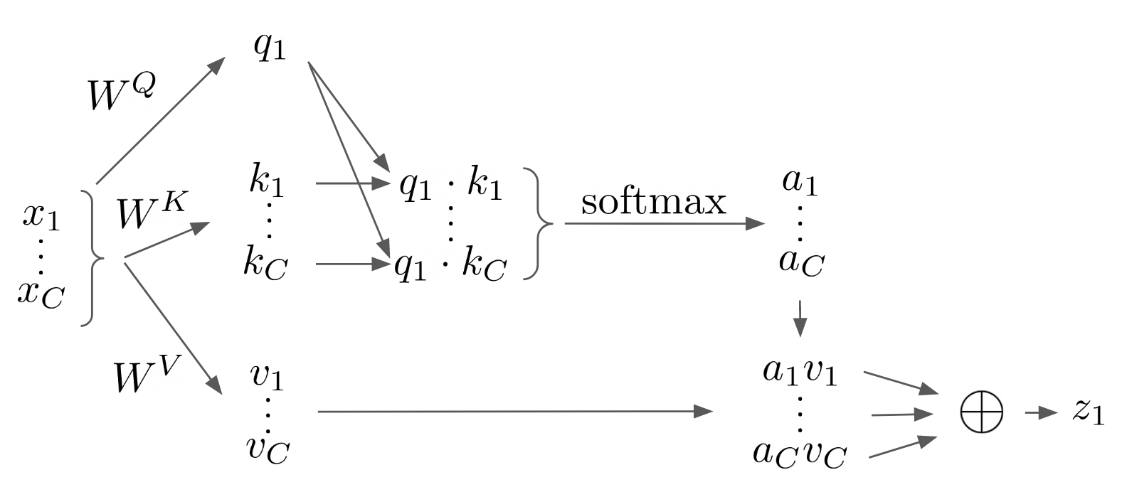
Figure 26: Illustration of single-headed self-attention. Figure from Ref. [23].

We start with single-headed self-attention illustrated in Fig. 26. Let us assume that we are again analyzing $C$ jet constituents, so the vector $x_{1}$ describes the phase space position for the first constituent in an unordered list. If we stick to an image-like representation, the complete vector $x$ will be $C$ copies of the 3-dimensional phase space vector given in Eq.(2.39). First, we define a latent or query representation of $x_{1}$ through a learned weight matrix $W^{Q}$,

$$q_{1}=W^{Q}x_{1}\;.$$ (2.55)

If we cover all constituents, $W^{Q}$ becomes a block-diagonal matrix of size $3C$. Next, to relate all constituents $x_{1}~{}...~{}x_{C}$ to $x_{1}$, we define a learned key matrix

$$\begin{pmatrix}k_{1}\\ \vdots\\ k_{C}\end{pmatrix}=W^{K}\begin{pmatrix}x_{1}\\ \vdots\\ x_{C}\end{pmatrix}$$ (2.56)

We then project all keys $k_{1}~{}...~{}k_{C}$ onto the latent representation of $x_{1}$, namely $q_{1}$, using a scalar product. Modulo some details this defines a set of, in our case, 3-dimensional vectors like

$$\begin{pmatrix}a_{1}^{(1)}\\ \vdots\\ a_{C}^{(1)}\end{pmatrix}=\text{Softmax}\begin{pmatrix}(q_{1}\cdot k_{1})\\ \vdots\\ (q_{1}\cdot k_{C})\end{pmatrix}\qquad\text{with}\quad a_{i}^{(1)}\in[0,1]\qquad\sum_{i}a_{i}^{(1)}=1\;,$$ (2.57)

all in reference to $x_{1}$. Finally, we transform the complete set of inputs $x_{1}~{}...~{}x_{C}$ into a latent value representation, in complete analogy to the constrained query form of Eq.(2.55), but allowing for full correlations,

$$\begin{pmatrix}v_{1}\\ \vdots\\ v_{C}\end{pmatrix}=W^{V}\begin{pmatrix}x_{1}\\ \vdots\\ x_{C}\end{pmatrix}\;,$$ (2.58)

through a third learned matrix $W^{V}$. This latent representation of the entire jet is then weighted with the $x_{1}$-specific vector $a^{(1)}$ to define the network output. Generalizing from $x_{1}$ to $x_{j}$ this gives us the output vector for the transformer-encoder layer

$$z_{j} =\sum_{i=1}^{3C}a_{i}^{(j)}v_{i}=\sum_{i}\text{Softmax}_{i}\Big{[}(W^{Q}x_{j})\cdot(W^{K}x_{i})\Big{]}\;(W^{V}x)_{i}\;.$$ (2.59)

This form can be thought of as constructing a new basis $v_{i}$, where the coefficients are given by $\text{Softmax}(q_{1},k_{i})$. The same operation applied to all $x_{j}$ defines the $3C$-dimensional output vector $z$. This formula also shows that the matrices $W^{Q}$ and $W^{K}$ do not have to be quadratic and can define internal representations $Wx$ with any number of dimensions. The size of $W^{V}$ defines the dimension of the output vector $z$. By construction, each output of our transformer-encoder $z_{i}$ is invariant to the permutation of the other elements of the set.

A practical problem with the self-attention described above is that each element tends to attend dominantly to itself, which means that in Eq.(2.57) the diagonal entries $a_{j}^{(j)}$ dominate. This numerical problem can be cured by extending the network to multiple heads, which means we perform several self-attention operations in parallel, each with separate learned weight matrices, and concatenate the outputs before applying a final linear layer. This might seem not efficient in computing time, but in practice we can do the full calculation for all constituents, all attention heads, and an entire batch in parallel with tensor operations, so it pays off.

Because a transformer can be viewed as a preprocessor for the jet constituents, enforcing permutation invariance before any kind of NN application, we can combine with it any other preprocessing step. For instance, we know that constituents with small $p_{T}$ just represent noise, either from QCD or from pileup, and they should have no effect on the physics of the subjet constituents. We can implement this constraint in a IR-safe transformer, where we add a correction factor to Eq.(2.57),

$$a_{j}^{(1)}=\text{Softmax}[(q_{i}\cdot k_{j})+\beta\log p_{T}]\;.$$ (2.60)

For small $p_{T}$ the second contribution ensures that constituents with $p_{T}\to 0$ do not contribute to the attention weights $a_{j}$. In addition, we replace $z_{j}\to p_{T,j}z_{j}$ in the transformer output.

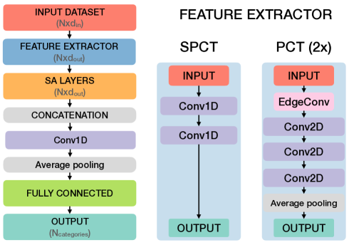
Figure 27: Network architecture and feature extractors for the top tagging application of the point cloud transformer. Figure from Ref. [24].

The transformer-encoder layer can then be used as part of different network architectures, for example to analyze jets. The output $z$ of a stack of transformer layers can be fed into a classification network directly, or it can be combined with the input features $x$, in the spirit of the skip connections discussed in Sec. 2.1.3, to define an offset-attention. In Fig. 27 we illustrate the combination of the transformer with two different feature extractors, a set of 1-dimensional convolutional layers running over the features $x$ of each constituent (SPCT), and an edge convolution as introduced in Sec. 2.3.2 (PCT). The edge convolution uses a large number of $k=20$ nearest neighbors and is followed by 2-dimensional convolutions. The output of the transformer layers is then concatenated to an expanded feature dimension and fed through a fully connected network to provide the usual classification output. This way the SPCT is an transformer-enhanced fully connected network and the PCT combines a simplified GCN structure with a transformer-encoder. The performance of the simple SCPT network matches roughly the standard CNN or LoLa results shown in Fig. 15, but with only 7k network parameters. The PCT performs almost as well as the leading ParticleNet architecture, but with only 200k instead of almost 500k network parameters. So while transformers with their different learned matrices appear parameter-intensive, they are actually efficient in reducing the size of the standard networks while ensuring permutation invariance as the key ingredient to successful jet tagging. The challenge of the transformer preprocessing is their long training time.

2.3.4 Deep sets

Motivated by the same argument of permutation invariance as the transformers, another approach to analyzing LHC jets and events is based on the mathematical observation that we can approximate any observable of 4-vectors using a combination of per-particle mappings and a continuous pooling function,

$$\{k_{\mu,i}\}\to F_{\theta}\left(\sum_{i}\Phi_{\theta}(k_{\mu,i})\right)$$ (2.61)

where $\Phi\in\mathbb{R}^{\ell}$ is a latent space representation of each input 4-vector or extended particle information. Latent spaces are abstract, intermediate spaces constructed by neural networks. By some kind of dedicated requirement, they organize the relevant information and form the basis for example of all generative networks discussed in Sec. 4. As a side remark, the observable $F$ can be turned infrared and collinear safe by replacing $\Phi(k_{\mu,i})\to p_{T,i}\Phi$, where $\Phi$ now only depends on the angular information of the $k_{\mu}$. This is the same strategy as the IR-safe transformer in Eq.(2.60). Such an IR-safe energy flow network (EFN) representation is an additional restriction, which means it will weaken the distinguishing power of the discriminative observable, but it will also make it consistent with perturbative QFT. In Tab. 2 we show a few such representations, including subjet observables from Eq.(1.6).

A particle flow network (PFN) implementation of the deep sets architecture is, arguably, the simplest way to analyze point clouds by using two networks. The first network constructs the latent representations respecting the permutation symmetry of the inputs. It is a simple, fully connected network relating the 4-vectors and the particle-ID, for the PFN-ID version, to a per-vector $\ell$-dimensional latent representation $\Phi_{\theta}(k_{\mu})\in\mathbb{R}^{\ell}$. The second, also fully connected network, sums the $\Phi_{\theta}$ for all 4-vectors just like the graph aggregation function in Eq.(2.50), and feeds them through a fully connected classification network with a softmax or sigmoid activation function as its last layer. The entire classification network is trained though a cross-entropy loss.

For the competitive top tagging results shown in Fig. 15 the energy flow network (EFN) and the particle flow network (PFN) only require 82k parameters in the two fully connected networks, with a 256-dimensional latent space. The suppression of QCD jets for a given top tagging efficiency is roughly 20% smaller when we require soft-collinear safety from the EFN rather than using the full information in the PFN.

		$\Phi$	$F$
mass	$m$	$p^{\mu}$	$F(x^{\mu})=\sqrt{x^{\mu}x_{\mu}}$
multiplicity	$n_{\text{PF}}$	$1$	$F(x)=x$
momentum dispersion	$p_{T}D$	$(p_{T},p_{T}^{2})$	$F(x,y)=\sqrt{y}/x$

Table 2: Example for observables decomposed into per-particle maps $\Phi$ and functions $F$ according to Eq.(2.61). In the last column, the arguments of $F$ are placeholders for the summed output of $\Phi$. Table from Ref. [25].

Just like for the graph network in Sec. 2.3.2 it is also clear how one would add information on the identified particles in a jet or an event. The question is how to best add additional entries to the $k_{\mu}$ introduced in Eq.(2.38). In analogy to the preprocessing of jet images, described in Sec. 2.1.2, we would likely use the $\eta$ and $\phi$ coordinates relative to the jet axis, combined with the (normalized) transverse momentum $p_{T}$. A fourth entry could then be the mass of the observed particle, if non-zero. The charge could simply be a fifth entry added to $k_{\mu}$. Particle identification would then tell us if a jet constituent is a

$$\gamma,e^{\pm},\mu^{\pm},\pi^{0},\pi^{\pm},K_{L},K^{\pm},n,p\cdots$$ (2.62)

One way to encode such categorical data would be to assign a number between zero and one for each of these particles and add a sixth entry to the 4-momentum. This is equivalent to assigning the particle code an integer number and then normalizing this entry of the feature vector. To learn the particle-ID the network then learns the ordering in the corresponding direction.

The problem with this encoding becomes obvious when we remind ourselves that a loss function forms a scalar number out of the feature vector, so the network needs to learn some kind of filter function to extract this information. This means combining different categories into one number is not helping the network. Another problem is a possible bias from the network architecture or loss function, leading to an enhanced sensitivity of the network to larger values of the particle-ID vector. Some ranges in the ID-directions might be preferred by the network, bringing us back to permutation invariance, the theme of this section. Instead, we can encode the particle-ID in a permutation-invariant manner, such that a simple unit vector in all directions can extract the information. Using one-hot encoding the phase space vector of Eq.(2.39) becomes

$$k_{\mu}\quad\to\quad\begin{pmatrix}\Delta\eta\\ \Delta\phi\\ p_{T}\\ m\\ \delta_{\text{ID}=\gamma}\\ \delta_{\text{ID}=e}\\ \vdots\end{pmatrix}\;.$$ (2.63)

The additional dimensions can only have entries zero and one. This method looks like a waste of dimensions, until we remind ourselves that a high-dimensional feature space is actually a strength of neural networks and that this kind of information is particularly easy to extract and de-correlate from the feature space.

2.4 Symmetries and contrastive learning

After observing the power of networks respecting permutation invariance, we can think about symmetries and neural network architectures more generally. Since Emmy Noether we know that symmetries are the most basic structure in physics, especially in particle physics. LHC physics is defined by an extremely complex symmetry structure, starting with LHC data, the detector geometry, to the relativistic space-time symmetries and local gauge symmetries defining the underlying QFT. If we want to use machine learning we need to embrace these symmetries. For instance, the jet or calorimeter images introduced in Sec. 2.1 are defined in rapidity vs azimuthal angle, observables inspired by Lorentz transformations and by the leading symmetry of the LHC detectors. The preprocessing of jet images exploits the rotation symmetry around the jet axis. The rather trivial case of permutation symmetry is driving all of the network architectures presented in Sec. 2.3. Theoretical invariances under infrared transformations motivated the IR-safe transformer and the energy flow networks.

From a structural perspective, there are two ways symmetries can affect neural networks. First, we call a network equivariant if for a symmetry operation $S$ and a network output $f_{\theta}(x)$ we have

$$f_{\theta}(S(x))=S(f_{\theta}(x))\;.$$ (2.64)

It means we can recover a symmetry operation $S$ on the data $x$ as a symmetry operation of an equivariant network output. For example, if we shift all pixels in an input image to a CNN in one direction, the training of the convolutional filters will not change and the feature maps inside the network will just be shifted as well, so the CNN is equivariant under translations. We would not want the network to be completely invariant to translations, because the main question in jet tagging is always where features appear relative to a fixed jet axis. An equivalent definition of an equivariant network is that for two different inputs with the same output, two transformed inputs also give the same output,

$$f_{\theta}(x_{1})=f_{\theta}(x_{2})\qquad\Rightarrow\qquad f_{\theta}(S(x_{1}))=S(f_{\theta}(x_{1}))=S(f_{\theta}(x_{2}))=f_{\theta}(S(x_{2}))\;.$$ (2.65)

A stronger symmetry requirement is an invariant network, namely

$$\boxed{f_{\theta}(S(x))=f_{\theta}(x)}\;.$$ (2.66)

The rotation step of the jet image preprocessing in Sec. 2.1.2 ensures the hard way that the classification network is rotation-invariant. Similarly, the goal of the Lorentz layer in Eq.(2.42) is to guarantee a Lorentz-invariant definition of the classification network. Finally, the goal of the graph-inspired networks discussed in Sec. 2.3 is to provide a network architecture which guarantees that the classification outcome is permutation invariant.

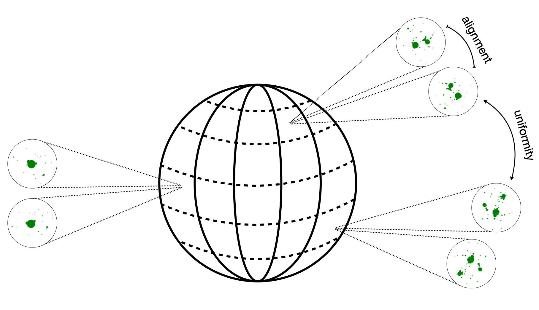
Figure 28: Illustration of the uniformity and alignment concepts behind the contrastive learning. Figure from Ref. [23].

For particle physics applications, it would be extremely cool to have a training procedure and loss function which ensures that the latent or representation space is invariant to pre-defined symmetries or invariances and still retains discriminative power. This means we could implement any symmetry requirement either through symmetric training data or through symmetric data augmentations. A way to achieve this is contrastive learning of representations (CLR). The goal of such a network is to map, for instance, jets $x_{i}$ described by their constituents to a latent or representation space,

$$f_{\theta}:\quad x_{i}\rightarrow z_{i}\;,$$ (2.67)

which is invariant to symmetries and theory-driven augmentations, and remains discriminative for the training and test datasets.

As usually, our jets $x_{i}$ are described by $n_{C}$ massless constituents and their phase space coordinates given in Eq.(2.39), so the jet phase space is $3n_{C}$-dimensional. We first take a batch of jets $\{x_{i}\}$ from the dataset and apply one or more symmetry-inspired augmentations to each jet. This generate an augmented batch $\{x_{i}^{\prime}\}$. We then pair the original and augmented jets into two datasets

positive pairs: $$\qquad\qquad\{(x_{i},x_{i}^{\prime})\}$$

negative pairs: $$\qquad\qquad\{(x_{i},x_{j})\}\cup\{(x_{i},x_{j}^{\prime})\}\quad\text{for}\quad i\neq j\;.$$ (2.68)

Positive pairs are symmetry-related and negative are not. The goal of the network training is to map positive pairs as close together in representation space as possible, while keeping negative pairs far apart. Simply pushing apart the negative pairs allows our network to encode any kind of information in their actual position in the latent space. Labels, for example indicating if the jets are QCD or top, are not used in this training strategy, which is referred to as self-supervised training. The trick to achieve this split in the representation space is to replace vectors $z_{i}$, which the network outputs, by their normalized counterparts,

$$f_{\theta}(x_{i})=\frac{z_{i}}{|z_{i}|}\qquad\text{and}\qquad f_{\theta}(x_{i}^{\prime})=\frac{z_{i}^{\prime}}{|z_{i}^{\prime}|}\;.$$ (2.69)

This way the jets are represented on a compact hypersphere, on which we can define the similarity between two jets as

$$s(z_{i},z_{j})=\frac{z_{i}\cdot z_{j}}{|z_{i}||z_{j}|}\in[-1,1]\;,$$ (2.70)

which is just the cosine of the angle between the jets in the latent space. This similarity is not a proper distance metric, but we could instead define an angular distance in terms of the cosine, such that it satisfies the triangle inequality. Based on this similarity we construct a contrastive loss. It can be understood in terms of alignment versus uniformity on the unit hypersphere, illustrated in Fig. 28. Starting with negative pairs, a loss term like

$$\boxed{\mathcal{L}_{\text{CLR}}\supset\sum_{j\neq i\in\text{batch}}\left[e^{s(z_{i},z_{j})/\tau}+e^{s(z_{i},z_{j}^{\prime})/\tau}\right]}$$ (2.71)

will be push them apart, preferring $s\to-1$, but on the compact hypersphere they cannot be pushed infinitely far apart. This means our loss will be minimal when the unmatched jets are uniformly distributed. To map the jets to such a uniform distribution in a high-dimensional space, the mapping will identify features to discriminate between them and map them to different points. We have seen this self-organization effect for the capsule networks in Sec. 2.2. Next, we want the loss to become minimal when for the positive pairs all jets and their respective augmented counterparts are aligned in the same point, $s\to 1$. This additional condition induces the invariance with respect to augmentations and symmetries. The contrastive loss is given by a sum of the two corresponding conditions

$$\mathcal{L}_{\text{CLR}} =-\sum_{i\in\text{batch}}\frac{s(z_{i},z_{i}^{\prime})}{\tau}+\sum_{i\in\text{batch}}\log\sum_{j\neq i\in\text{batch}}\left[e^{s(z_{i},z_{j})/\tau}+e^{s(z_{i},z_{j}^{\prime})/\tau}\right]$$

$$=-\sum_{i\in\text{batch}}\log\frac{e^{s(z_{i},z_{i}^{\prime})/\tau}}{\sum_{j\neq i\in\text{batch}}\left[e^{s(z_{i},z_{j})/\tau}+e^{s(z_{i},z_{j}^{\prime})/\tau}\right]}\;,$$ (2.72)

The so-called temperature $\tau>0$ controls the relative influence of positive and negative pairs. The first term sums over all positive pairs and reaches its minimum in the alignment limit. The negative pairs contribute to the second term, and the expression in brackets is summed over all negative-pair partners of a given jet. If such a solution were possible, the loss would force all individual distances to their maximum. For the spherical latent space the best the network can achieve is the smallest average $s$-value for a uniform distribution.

Next, we can apply contrastive learning to LHC jets, to see if the network learns an invariant representation and defines some kind of structure through the uniformity requirement. Before applying symmetry transformations and augmentations we start preprocessing the jets as described in Sec.2.1.2 and ensure that the $p_{T}$-weighted centroid is at the origin in the $\eta-\phi$ plane. Now, rotations around the jet axes are a very efficient symmetry we can impose on our representations. We apply them to a batch of jets by rotating each jet by angles sampled from $0~{}...~{}2\pi$. Such rotations in the $\eta-\phi$ plane are not Lorentz transformations and do not preserve the jet mass, but for narrow jets with $R\lesssim 1$ the corrections to the jet mass can be neglected. As a second symmetry we implement translations in the $\eta-\phi$ plane. Here, all constituents in a jet are shifted by the same random distance, where shifts in each direction are limited to $-1~{}...~{}1$.

In addition to (approximate) symmetries, we can also use theory-inspired augmentations. QFT tells us that soft gluon radiation is universal and factorizes from the hard physics in the jet splittings. To encode this invariance in the latent representation, we augment our jets by smearing the positions of the soft constituents, in $\eta$ and $\phi$ using from a Gaussian distribution centered on the original coordinates

$$\eta^{\prime}\sim\mathcal{N}\left(\eta,\frac{\Lambda_{\text{soft}}}{p_{T}}\right)\qquad\text{and}\qquad\phi^{\prime}\sim\mathcal{N}\left(\phi,\frac{\Lambda_{\text{soft}}}{p_{T}}\right)\;,$$ (2.73)

with a $p_{T}$-suppression in the variance relative to $\Lambda_{\text{soft}}=100$ MeV. Secondly, collinear splittings lead to divergences in perturbative QFT. In practice. they are removed through the finite angular resolution of a detector, which cannot resolve two constituents with $p_{T,a}$ and $p_{T,b}$ at vanishing $\Delta R_{ab}\ll 1$. We introduce collinear augmentations by splitting individual constituents such that the total $p_{T}$ in an infinitesimal region of the detector is unchanged,

$$p_{T}\to p_{T,a}+p_{T,b}\qquad\text{with}\qquad\eta_{a}=\eta_{b}=\eta\qquad\phi_{a}=\phi_{b}=\phi\;.$$ (2.74)

These soft and collinear augmentations will enforce a learned IR-safety in the jet representation, unlike the modified versions of the transformer or the EFPs.

Finally, we include the permutation symmetry among the constituents, for instance through a transformer-encoder. The combination of contrastive loss and a permutation-invariant network architecture defines the JetCLR approach.

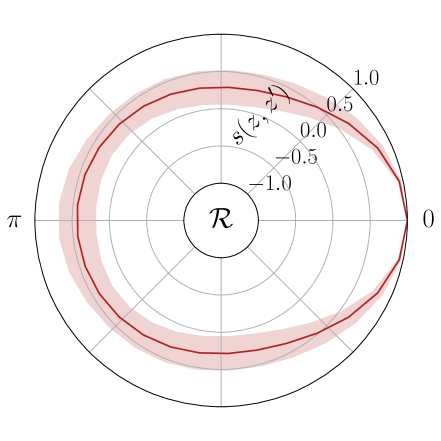
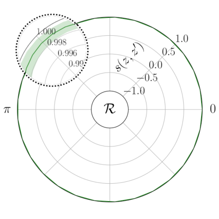
Figure 29: Visualization of the rotational invariance in representation space, where $s(z,z^{\prime})=1$ indicates identical representations. We compare JetCLR representations trained without (left) and with (right) rotational transformations. Figure from Ref. [23].

For a test sample of jets we can check if our JetCLR network indeed encodes symmetries. To illustrate the encoded rotation symmetry we show how the representation is invariant to actual rotations of jets. We start with a batch of 100 jets, and produce a set of rotated copies for each jet, with rotation angles evenly spaced in $0~{}...~{}2\pi$. We then pass each jet and its rotated copy through the JetCLR network, and calculate their similarity in the latent representation, Eq.(2.70). In Fig. 29 we show the mean and standard deviation of the similarity as a function of the rotation angle without and with the rotational symmetry included in the JetCLR training. In the left panel the similarity varies between $0.5$ and $1.0$ as a function of the rotation angle, while in the right panel the JetCLR representation is indeed rotationally invariant. From the scale of the radial axis $s(z,z^{\prime})$ we see that the representations obtained by training JetCLR with rotations are very similar to the original jets.

Augmentation	$\epsilon^{-1}(\epsilon_{s}\!=\!0.5)$	AUC
none	15	0.905
translations	19	0.916
rotations	21	0.930
soft+collinear	89	0.970
combined	181	0.979

Table 3: JetCLR classification results for different symmetries and augmentations and $S/B\!=\!1$. The combined setup includes translation and rotation symmetries, combined with soft and collinear augmentations. Table from Ref. [23].

Before using the JetCLR construction for an explicit task, we can can analyze the effect of the different symmetries and theory augmentations using a linear classifier test (LCT). For this test we train a linear neural network with a binary cross-entropy loss to distinguish top and QCD jets, while our JetCLR training does not know about these labels. This means the LCT tells us if the uniformity condition has encoded some kind of feature which we assume to be correlated with the difference between QCD and top jets. A high AUC from the LCT points to a well-structured latent representation. From first principles, it is not clear which symmetries and augmentations work best for learning representations. In Tab. 3 we summarize the results after applying rotational and translational symmetry transformations and soft+collinear augmentations. It turns our that, individually, the soft+collinear augmentation works best. Translations and rotations are less powerful individually, but the combination defines by far the best-ordered representations.

3 Non-supervised classification

Searches for BSM physics at the LHC traditionally start with a theory hypothesis, such that we can compare the expected signature with the Standard Model background prediction for a given phase space region using likelihood methods. The background hypothesis might be defined through simulation or through an extrapolation from a background into a signal region. This traditional approach has two fundamental problems which we will talk about in this section and which will take us towards a more modern interpretation of LHC searches.

First, we can generalize classification, for example of LHC events, to the situation where our training data is measured data and therefore does not come with event-wise labels. However, a standard assumption of essentially any experimental analysis is that signal features are localized in phase space, which means we can define background regions, where we assume that there is no signal, and signal regions, where there still are background, but accompanied by a sizeable signal fraction. This leads us to classification based on weakly supervised learning.

Second, any searches based on hypothesis testing does not generalize well in model space, because we can never be sure that our model searches actually cover an existing anomaly or sign of physics beyond the Standard Model. We can of course argue that we are performing such a large number of analyses that it is very unlikely that we will miss an anomaly, but this approach is at the very least extremely inefficient. We also need to remind ourselves that ruling out some parameter space in a pre-defined model is not really a lasting result. This means we should find ways to identify for example anomalous jets or events in the most model-independent way. Such a method can be purely data-driven or rely on simulations, but in either case we only work with background data to extract an unknown signal, a method refereed to as unsupervised learning.

3.1 Classification without labels

Until now we have trained classification networks on labelled, pure datasets. Following the example of top tagging in Sec. 2.1.1, such training data can be simulations or actual data which we understand particularly well. The problem is that in most cases cases we do not understand a LHC dataset well enough to consider it fully labelled. What is much easier is to determine the relative composition of such a dataset with the help of simulations, for instance 80% top jets combined with 20% QCD jets on the one hand and 10% top jets combined with 90% QCD jets on the other.

Let us go back to Sec. 1.2.1 where we looked at phase space distributions of signal and background jets or events $p_{S,B}(x)$. What we observe are not labelled signal and background samples, but two mixed samples with global signal fractions $f_{1,2}$ and background fractions $1-f_{1,2}$ in our two training datasets. The mixed phase space densities $p_{1,2}$ are related to the pure densities as

$$\begin{pmatrix}p_{1}(x)\\ p_{2}(x)\end{pmatrix} =\begin{pmatrix}f_{1}&1-f_{1}\\ f_{2}&1-f_{2}\end{pmatrix}\begin{pmatrix}p_{S}(x)\\ p_{B}(x)\end{pmatrix}$$

$$\Leftrightarrow\qquad\begin{pmatrix}p_{S}(x)\\ p_{B}(x)\end{pmatrix} =\frac{1}{f_{1}-f_{2}}\begin{pmatrix}1-f_{2}&f_{1}-1\\ -f_{2}&f_{1}\end{pmatrix}\begin{pmatrix}p_{1}(x)\\ p_{2}(x)\end{pmatrix}$$

$$\Rightarrow\qquad\;\frac{p_{S}(x)}{p_{B}(x)} =\frac{(1-f_{2})p_{1}(x)+(f_{1}-1)p_{2}(x)}{-f_{2}p_{1}(x)+f_{1}p_{2}(x)}\;.$$ (3.1)

The last line implies that, if we know $f_{1,2}$ and can also extract the mixed densities $p_{1,2}(x)$ of the two training datasets, we can compute the signal and background distributions and with them the likelihood ratio as the optimal test statistics.

Next, we can ask the question how the likelihood ratios for signal vs background classification, $p_{S}/p_{B}$, and the separation of the two mixed samples, $p_{1}/p_{2}$, are related. This will lead us to a shortcut in our classification task,

$$\frac{p_{1}(x)}{p_{2}(x)} =\frac{f_{1}p_{S}(x)+(1-f_{1})p_{B}(x)}{f_{2}p_{S}(x)+(1-f_{2})p_{B}(x)}=\frac{f_{1}\dfrac{p_{S}(x)}{p_{B}(x)}+1-f_{1}}{f_{2}\dfrac{p_{S}(x)}{p_{B}(x)}+1-f_{2}}$$

$$\frac{d}{d(p_{S}/p_{B})}\frac{p_{1}(x)}{p_{2}(x)} =\frac{f_{1}\left[f_{2}\dfrac{p_{S}(x)}{p_{B}(x)}+1-f_{2}\right]-f_{2}\left[f_{1}\dfrac{p_{S}(x)}{p_{B}(x)}+1-f_{1}\right]}{\left[f_{2}\dfrac{p_{S}(x)}{p_{B}(x)}+1-f_{2}\right]^{2}}=\frac{f_{1}-f_{2}}{\left[f_{2}\dfrac{p_{S}(x)}{p_{B}(x)}+1-f_{2}\right]^{2}}\;.$$ (3.2)

The sign of this derivative is a global $\text{sign}(f_{1}-f_{2})$ and does not change if we vary the likelihood ratios. This means the two likelihood ratios are linked through a monotonous function, which means that we can exchange them as a test statistics at no cost. In other words, if we are interested in an optimal classifier we can skip the translation into $p_{S}/p_{B}$ and just use the classifier between the two mixed samples, $p_{1}/p_{2}$, instead. This is an attractive option, because it means that we do not need to know $f_{1,2}$ if we are just interested in the likelihood ratio.

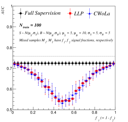
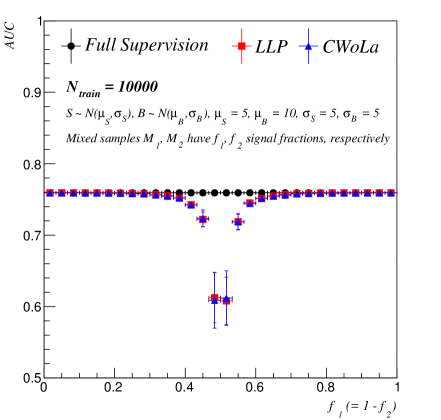
Figure 30: Performance of the CWoLa method for the double-Gaussian toy example as a function of the signal fraction in one of the training datasets for 100 (left) and 10000 (right) training points. Figure from Ref. [26].

While this classification without labels (CWoLa) does not require use to know the signal and background fractions and is therefore, strictly speaking, an unsupervised method, we always work under the assumption that we have a background-dominated and a signal-dominated dataset. Moreover, any such analysis tool needs to be calibrated. If the classification outcome is not a signal or background probability, as discussed in Sec. 2, we need to define a working point for our classifier and determine its signal and background efficiencies. From Eq.(3.1) we see that we only need two samples with known signal and background fractions to extract $p_{S}(x)$ and $p_{B}(x)$ for any given working point.

We illustrate the unsupervised method using the original toy model of a 1-dimensional, binned observable $x$ and Gaussian signal and background distributions $p_{S,B}(x)=\mathcal{N}(x)$. We have three options to train a classifier on this dataset, which means we can

1. compute the full supervised likelihood ratio $p_{S}/p_{B}(x)$ from the truth distributions;

2. use Eq.(3.1) to compute the likelihood ratio from $p_{1,2}(x)$ and known label proportions $f_{1,2}$ (LLP);

3. follow the CWoLa method and use $p_{1}/p_{2}(x)$ to separate signal and background instead of the two samples.

The AUC values for the three methods are shown in Fig. 30 as a function of the signal fraction of one of the two samples, chosen the same as the background fraction for the second sample. The horizontal dashed line indicates the fully-supervised AUC with infinite training statistics. By construction, the AUC for full supervision is independent of $f_{1}$. The weakly supervised and unsupervised methods start coinciding with the fully supervised method as long as we stay away from

$$f_{1}\approx f_{2}\approx\frac{1}{2}\;.$$ (3.3)

We can see the problem with this parameter point in Eq.(3.1), where a matrix inversion is not possible. Similarly, in Eq.(3.2) the linear dependence of the two likelihood ratios vanishes in the same parameter point.

For jet tagging the CWoLa method becomes relevant when we cannot construct pure training samples for either experimental or theoretical reasons. As discussed above, the standard top tagging benchmark is chosen to be well defined theoretically and experimentally. This is different for quark vs gluon tagging. However, quark–gluon tagging is experimentally extremely attractive, because it would for instance allow us to suppress backgrounds to the weak-boson-fusion processes discussed in Sec. 1.2.1. On the theory side, we know that partons split into pairs of collinear daughter partons with a probability described by the unregularized splitting kernels

$$\hat{P}_{g\leftarrow g}(z) =N_{c}\;\left[\frac{z}{1-z}+\frac{1-z}{z}+z(1-z)\right] \qquad\hat{P}_{q\leftarrow g}(z) =\frac{1}{2}\;\big{[}z^{2}+(1-z)^{2}\big{]}$$

$$\hat{P}_{g\leftarrow q}(z) =\frac{N_{c}^{2}-1}{2N_{c}}\;\frac{1+(1-z)^{2}}{z} \qquad\hat{P}_{q\leftarrow q}(z) =\frac{N_{c}^{2}-1}{2N_{c}}\;\frac{1+z^{2}}{1-z}$$ (3.4)

where $z$ is the energy fraction carried by the harder of the two daughter partons which also describes the splitting $\hat{P}_{j\leftarrow i}$. The off-diagonal splitting probabilities imply that partonic quarks and gluons are only defined probabilistically, which means any kind of quark-gluon tagging at the LHC will at most be weakly supervised. Another theoretical complication is that quarks pairs coming for example from a large-angle gluon splitting $g\to q\bar{q}$ and from an electroweak decay $Z\to q\bar{q}$ have different color-correlations, so they are not really identical at the single-quark level. Experimentally, it is also impossible to define pure quark vs gluon jets samples. While most LHC jets at moderate energies are gluons, we can use $W$ and $Z$ decays to collect quark jets, but some of those decays actually include three or more jets, $Z\to q\bar{q}g$, which again leads us to learn from mixed samples.

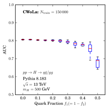
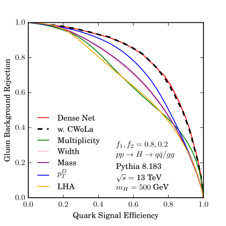
Figure 31: Performance of the CWoLa method for quark-gluon tagging as a function of the signal fraction (left), and the corresponding ROC curve (right). Figure from Ref. [26].

We can apply CWoLa to quark-gluon tagging, using a very simple classification network based on five substructure observables like those shown in Eq.(1.6). To simplify things, the jets are generated from hypothetical Higgs decays with $m_{H}=500$ GeV

$$pp\to H\to qq\;/\;q\bar{q}\;.$$ (3.5)

Again we train the network on two mixed samples and show the results in Fig. 31. In this example, we do not extract the likelihood ratio, but train a standard classifier to separate the two training samples by minimizing the cross entropy. We then apply the classifier to split signal and background, so we rely on the fact that our network knows the Neyman-Pearson lemma. For the exact relation between a trained discriminator and the likelihood ratio we refer to Sec. 4.2.1. In the left panel we see that the AUC is again stable as long as we stay away from equally mixed training samples. In the right panel we see that the performance of the network is as good as the same network trained on labelled data.

Another application of CWoLa would be event classification, where we associate a signal with a specific phase space configuration which can also be generated by background processes. This is an example for LHC analyses not based on detailed hypothesis tests. A search with a minimal model dependence is a bump hunt in the invariant mass of a given pair of particles. Looking for a resonance decaying to two muons or jets we get away with minimum additional assumptions, for example on the underlying production process or correlations with other particles in the final state, by letting a mass window slide through the invariant mass distribution and searching for a feature in this smooth observable. Technically, we can analyse a binned distribution by fitting a background model, taking out individual bins, and checking if $\chi^{2}$ changes. The reason why this method works is that we have many data points in the background regions and a localized signal region, which can be covered by the background model through interpolation. This analysis idea is precisely what we have in mind for an enhanced classification network with weakly supervised or unsupervised training.

Looking at our usual reference process, there exists no point in the signal phase space for the process

$$pp\to t\bar{t}H\to t\bar{t}\;(b\bar{b})$$ (3.6)

which is not also covered by the $t\bar{t}b\bar{b}$ continuum background. The only difference is that in background regions like $m_{bb}=50~{}...~{}100$ GeV or $m_{bb}>150$ GeV there will be hardly any signal contamination while under the Higgs mass peak $m_{bb}\sim 125$ GeV the signal-to-background ratio will be sizeable. This separation might appear trivial, but the mass selection will propagate into the entire phase space. This means we can use sidebands to extract the number of background events expected in the signal region and subtract the background from the combined $m_{bb}$ distribution. If we want to subtract the background event by event over the entire phase space, we need to include additional information from the remaining phase space directions, ideally encoded in an event-by-event classifier.

For a signal-background separation using the kind of likelihood-based classifier described above we need two mixed training samples. We can use the $m_{bb}$ distribution to define two event samples, one with almost only background events and one with an enhanced signal fraction. The challenge of such a construction is that over the entire phase space the mixed samples need to be based on the same underlying signal and background distributions $p_{S,B}(x)$, just with different signal fractions $f_{1,2}$, as introduced in Eq.(3.1). This means that if we assume that the distribution of all phase space features $x$, with the exception of $m_{bb}$, are the same for signal and background, a CWoLa classifier will detect the signal correctly. This is a strong assumption, and we will revisit this challenge in Sec. 5.3.2 in the context of density estimation.

Finally, on a slightly philosophical note we can argue that it is difficult to separate signal from background events in a situation where both processes are defined though transition amplitudes over phase space and will interfere. Still, in this case we can define a background label for all events which remain in the limit of zero signal strength and a signal label to the pure signal and the interference with the background. Note that the interference can be constructive or destructive for a given phase space point.

3.2 Anomaly searches

The main goal of the LHC is to search for new and interesting effects which would require us to modify our underlying theory. If BSM physics is accessible to the LHC, but more elusive than expected, we should complement our hypothesis-based search strategies with more general approaches. For example, we can search for jets or events which stick out by some measure, turning them into prime candidates for a BSM physics signature. If we assume that essentially all events or jets at the LHC are described well by the Standard Model and the corresponding simulations, such an outlier search is equivalent to searching for the most non-SM instances. The difference between these two statements is that the first is based on unlabeled data, while the second refers to simulations and hence pure SM samples. They are equivalent if the data-based approach effectively ignores the outliers in the definition of the background-like sample and its implicitly underlying phase space density.

3.2.1 (Variational) autoencoders

For the practical task of anomaly searches, autoencoders (AEs) are the simplest unsupervised ML-tool. In the AE architecture an encoder compresses the input data into a bottleneck, encoding each instance of the dataset in an abstract space with a dimension much smaller than the dimension of the input data. A decoder then attempts to reconstruct the input data from the information encoded in the bottleneck. This architecture is illustrated in the upper left panel of Fig. 32 and works for jets using an image or 4-vector representation. The loss function for such an AE can be the MSE defined in Eq.(1.22), quantifying the agreement of the pixels in an input jet image $x$ and the average jet image output $x^{\prime}$, summed over all pixels,

$$\mathcal{L}_{\text{MSE}}=\frac{1}{N}\sum_{i=1}^{N}\;\left|x_{i}-x_{i}^{\prime}\right|^{2}\;.$$ (3.7)

This sum is just an expectation value over a batch of jet images sampled from the usual data distribution $p_{\text{data}}(x)$,

$$\boxed{\mathcal{L}_{\text{MSE}}=\Big{\langle}\left|x-x^{\prime}\right|^{2}\Big{\rangle}_{p_{\text{data}}}}\;.$$ (3.8)

The idea behind the anomaly search is that the AE learns to compress and reconstruct the training data very well, but different test data passed through the AE results in a large loss.

Because AEs do not induce a structure in latent space, we have no choice but to use this reconstruction error or loss also as the anomaly score. This corresponds to a definition of anomalies as an unspecific kind of outliers. Using the latent loss as an anomaly score leads to a conceptual weakness when we switch the standard and anomalous physics hypothesis. For example, QCD jets with a limited underlying physics content of the massless parton splittings given in Eq.(3.4) can be described by a small bottleneck. An AE trained on QCD jets will not be able to describe top-decay jets with their three prongs and massive decays. Turning the problem around, we can train the AE on top jets, in which case it will be able to describe multi-prong topologies as well as frequently occurring single-prong topologies in the top sample. QCD jets are now just particularly simple top jets, which means that they will not lead to a large anomaly score. This bias towards identifying more complex data is also what we expect from the standard use of a bottleneck for data compression.

Moving beyond purely reconstruction-based autoencoders, variational autoencoders (VAEs) add structure to the latent bottleneck space, again illustrated in Fig. 32. In the encoding step, a high-dimensional data representation is mapped to a low-dimensional latent distribution, from which the decoder learns to generate the original, high-dimensional objects. The latent bottleneck space then contains structured information which might not be apparent in the high-dimensional input representation. This means the VAE architecture consists of a learnable encoder with the output distribution $z\sim E_{\theta}(z|x)$ mapping the phase space $x$ to the latent space $z$, and a learnable decoder with the output distribution $x\sim D_{\theta}(x|z)$. The loss combines two terms

$$\boxed{\mathcal{L}_{\text{VAE}}=\Big{\langle}-\big{\langle}\log D_{\theta}(x|z)\big{\rangle}_{E_{\theta}(z|x)}+\beta_{\text{KL}}D_{\text{KL}}[E_{\theta}(z|x),p_{\text{latent}}(z)]\Big{\rangle}_{p_{\text{data}}}}\;.$$ (3.9)

The first terms is the reconstruction loss, where we compute the likelihood of the output of the decoder $D_{\theta}(x|z)$ and given the encoder $E_{\theta}(z|x)$, evaluated on batches sampled from $p_{\text{data}}$. We get back the MSE version serving as the AE reconstruction loss in Eq.(3.8) when we approximate the decoder output $D_{\theta}(x|z)$ as a Gaussian with a constant width. The second term is a latent loss, comparing the latent-space distribution from the encoder to a prior $p_{\text{latent}}(z)$, which defines the structure of the latent space.

For a Gaussian prior we use the so-called re-parametrization trick to pretend to sample from any multi-dimensional Gaussian with mean $\mu$ and standard deviation $\sigma$ by instead sampling from a standard Gaussian

$$z=\mu+\sigma\;\epsilon\qquad\text{with}\qquad\epsilon\sim\mathcal{N}_{\mu=0,\sigma=1}\;.$$ (3.10)

For such a standard Gaussian prior $p_{\text{latent}}(z)$ and a Gaussian encoder output $E_{\theta}(z|x)$ the KL-divergence defined in Eq.(1.10) turns into the form of Eq.(1.47)

$$D_{\text{KL}}[E_{\theta}(z|x),\mathcal{N}_{0,1}]=\frac{1}{2n}\sum_{i=1}^{n}\left(\sigma_{i}^{2}+\mu_{i}^{2}-1-2\log\sigma_{i}\right),$$ (3.11)

where $\sigma_{i}$ and $\mu_{i}$ replace the usual $n$-dimensional encoder output $z$ for a given $x$. Combining the simple MSE-reconstruction loss of Eq.(3.7) with this form of the latent loss gives us an explicit form of the VAE loss for a batch of events or jet images.

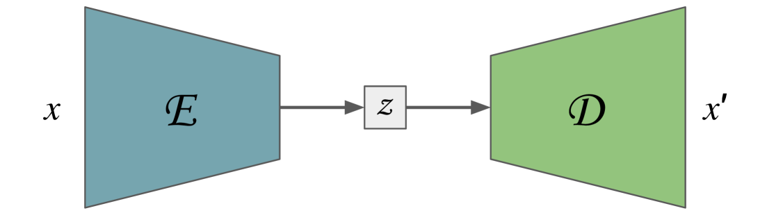
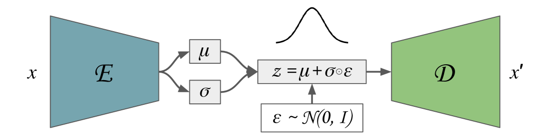
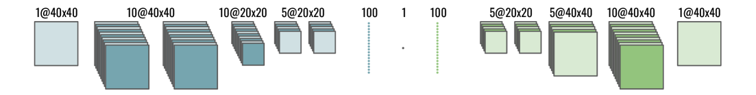
(a) Encoder and decoder

Figure 32: Architectures used for AE (left) and VAE (right) networks. All convolutions use a 5x5 filter size and all layers use PReLU activations. Downsampling from 40x40 to 20x20 is achieved by average pooling, while upsampling is nearest neighbor interpolation. Figure from Ref. [27].

Because of the structured bottleneck we now have a choice of anomaly scores, either based on the reconstruction or the latent space. This way the VAE can avoid the drawbacks of the AE by using an alternative anomaly score to the reconstruction error. We can compare the alternative choices using the standard QCD and top jet-images with a simple preprocessing described in Sec. 2.1.2. To force the network to learn the class the jet belongs to and to be able to visualize this information, we restrict the bottleneck size to one dimension. In the VAE case this gives us a useful probabilistic interpretation, since the mapping to the encoded space is performed by a probability distribution $E_{\theta}(z|x)$. To simplify the training of the classifier, we train on a sample with equal numbers of top and QCD jets. We are interested in three aspects of the VAE classifiers: (i) performance as a top-tagger, (ii) performance as a QCD-tagger, (iii) stable encoding in the latent space. Some results are shown in Fig. 33. Compared to the AE results, the regularisation of the VAE latent space generates as relatively stable and structured latent representation, even converging to a representation in which the top jets are clustered slightly away from the QCD jets. On the other hand, the separation in the VAE latent space is clearly not sufficient to provide a competitive anomaly score.

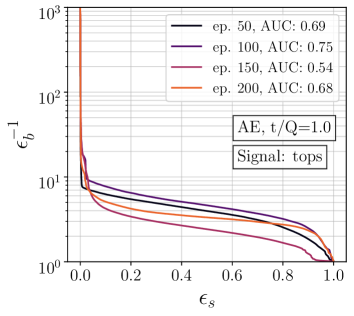
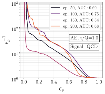
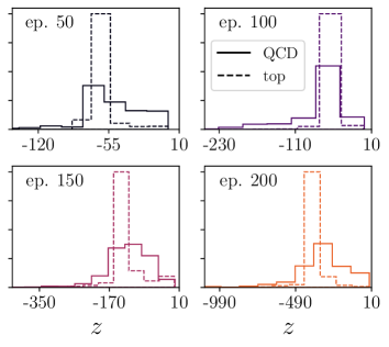
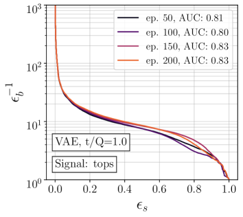
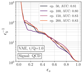
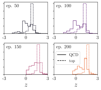
Figure 33: Symmetric performance of the toy-AE (upper) and toy-VAE (lower). In the large panels we show the ROC curves for tagging top and QCD as signals. In the small panels we show the distributions of top and QCD jets in the 1-dimensional latent space. Figure from Ref.[27].

For an unsupervised signal vs background classification a natural assumption for the latent space would be a bi-modal or multi-model structure. This is not possible for a VAE with a unimodal Gaussian prior, but we can try imposing an uncorrelated Gaussian mixture prior on the $n$-dimensional latent space. The GMVAE then minimizes the same loss as the VAE given in Eq.(3.9). However, for the regularization term we cannot calculate the KL-divergence analytically anymore. Instead, we estimate it using Monte Carlo integration and start by re-writing it according to its definition in Eq.(1.10)

$$D_{\text{KL}}[E_{\theta}(z|x),p_{\text{latent}}(z)]=\big{\langle}\log E_{\theta}(z|x)\big{\rangle}_{E_{\theta}(z|x)}-\big{\langle}\log p_{\text{latent}}(z)\big{\rangle}_{E_{\theta}(z|x)}\;.$$ (3.12)

For an arbitrary number of Gaussians the combined likelihood prior is given by

$$p_{\text{latent}}(z) =\sum_{r}p(z;r)\;p_{r}$$

$$\text{with}\qquad p(z;r) =\prod_{i=1}^{n}\;\frac{1}{\sqrt{2\pi}\sigma_{r,i}}\;\exp\left(-\frac{(z_{i}-\mu_{r,i})^{2}}{2\sigma^{2}_{r,i}}\right)$$ (3.13)

where $p_{r}$ is the weight of the respective mixture component $\mu_{r,i}$ is the mean of mixture component $r=1~{}...~{}R$ in dimension $i$, and $\sigma^{2}_{r,i}$ is the corresponding variance. All means, variances, and mixture weights are learned network parameters.

The problem with the GMVAE is that it does not work well for unsupervised classification. When training a 2-component mixture prior on our jet dataset the mixture components tend to collapse onto a single mode. To prevent this, we need to add a repulsive force between the modes, calculated as a function of the Ashman distance between two Gaussian distributions in one dimension,

$$D^{2}=\frac{2(\mu_{1}-\mu_{2})^{2}}{\sigma^{2}_{1}+\sigma^{2}_{2}}\;.$$ (3.14)

A value of $D>2$ indicates a clear mode separation. We encourage bi-modality in our latent space by adding the loss term

$$\mathcal{L}_{\text{GMVAE}}=\mathcal{L}_{\text{VAE}}-\lambda\tanh\frac{D}{2}\;.$$ (3.15)

The tanh function is meant to eventually saturate and stop pushing apart the modes. To cut the long story short, the Gaussian mixture prior will shape the latent space for the top vs QCD application and lead to a stable training. However, there is no increase in performance in going from the VAE to the GMVAE. The reason for this is that while the top jets occupy just one mode in latent space, the QCD jets occupy both. The mode assignment is mostly based on the amount of pixel activity within the jet, rather than on specific jet features. This means we need to go beyond the GMVAE in that we need a network which distributes the signal and background into the two different modes.

3.2.2 Dirichlet-VAE

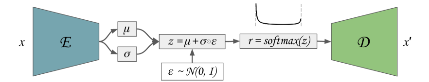
Figure 34: Architecture for the Dirichlet VAE. The approximate Dirichlet prior is indicated by the softmax step and the bi-modal distribution shown above it. Figure from Ref.[27].

The motivation, but ultimate failure of the GMVAE leads us to another way of defining a VAE with a geometry that leads to a mode separation. We can use the Dirichlet distribution, a family of continuous multivariate probability distributions, as the latent space prior,

$$\mathcal{D}_{\alpha}(r)=\frac{\Gamma(\sum_{i}\alpha_{i})}{\prod_{i}\Gamma(\alpha_{i})}\;\prod_{i}r_{i}^{\alpha_{i}-1},\qquad\text{with}\;i=1~{}...~{}R\;.$$ (3.16)

This $R$-dimensional Dirichlet structure is defined on an $R$-dimensional simplex, which means that all but one of the $r$ vector components are independent and $\sum_{i}r_{i}=1$. In our simple example with $R=2$ the latent space is described by $r_{1}\in[0,1]$, with $r_{0}=1-r_{1}$. The weights $\alpha_{i}>0$ can be related to the expectation values for the sampled vector components,

$$\langle r_{i}\rangle=\frac{\alpha_{i}}{\sum_{j}\alpha_{j}}\;,$$ (3.17)

which means that the Dirichlet prior it will create a hierarchy among different mixture components. An efficient way to generate numbers following a Dirichlet distributions is through a softmax-Gaussian approximation,

$$r\sim\text{softmax}\,\mathcal{N}(z;\tilde{\mu},\tilde{\sigma}) \approx\mathcal{D}_{\alpha}(r)$$

$$\text{with}\quad\tilde{\mu}_{i} =\log\alpha_{i}-\frac{1}{R}\sum_{i}\log\alpha_{i}$$

$$\tilde{\sigma}_{i} =\frac{1}{\alpha_{i}}\left(1-\frac{2}{R}\right)+\frac{1}{R^{2}}\sum_{i}\frac{1}{\alpha_{i}}\;.$$ (3.18)

The loss function of the Dirichlet-VAE (DVAE) includes the usual reconstruction loss and latent loss. For the higher-dimensional reconstruction loss we can use the cross-entropy between the inputs and the outputs, while the latent loss is given by the KL-divergence between the per-jet latent space representation and the Dirichlet prior. This is easily calculated for the Gaussians in the softmax approximation of the Dirichlet distribution and the Gaussians defined by the encoder output

$$\boxed{\mathcal{L}_{\text{DVAE}}=\Big{\langle}-\big{\langle}\log D_{\theta}(x|r)\big{\rangle}_{E_{\theta}(r|x)}+\beta_{\text{KL}}D_{\text{KL}}[E_{\theta}(r|x),\mathcal{D}_{\alpha}(r)]\Big{\rangle}_{p_{\text{data}}}}\;,$$ (3.19)

where the KL-divergence can be evaluated using Eq.(1.47). This way, training the DVAE is essentially equivalent to the standard VAE with its loss given in Eq.(3.9).

With a Dirichlet latent space the sampled $r_{i}$ can be interpreted as mixture weights of mixture components describing the jets. If we view the DVAE as a classification tool for a multinomial mixture model, these mixture components correspond to probability distributions over the image pixels. These distributions enter into the likelihood function of the model, which is parameterised by the decoder network. For our 2-dimensional example, the pure component distributions are given by $D_{\theta}(x|r_{1}=0)$ and $D_{\theta}(x|r_{1}=1)$, and any output for $r_{1}\in[0,1]$ is a combination of these two distributions. Our simple decoder architecture exactly mimics this scenario.

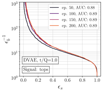
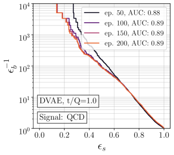
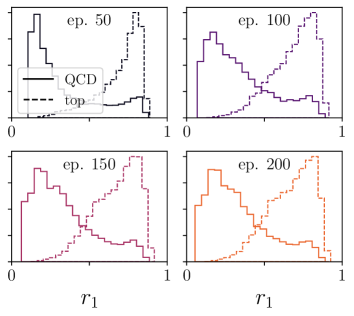
Figure 35: Results for the DVAE with $\alpha_{1,2}=1$. In the large panels we show the ROC curves for tagging top and QCD as signal. In the small panels we show the distributions of the top and QCD jets in the latent space developed over the training. Figure from Ref.[27].

To compare with the AE and VAE studies in Fig. 33 we can again train the DVAE on a mixture of QCD and top jets. We look for symmetric patterns in QCD and top tagging and show the latent space distributions in Fig. 35. First of all, the DVAE combined with its latent-space anomaly score identifies anomalies in both directions. The reason for this can be seen in the latent space distributions, which quickly settles into a bi-modal pattern with equal importance given to both modes. The QCD mode peaks at $r_{1}=0$, indicating that the $D_{\theta}(x|r_{1}=0)$ mixture describes QCD jets, while the top mode peaks at $r_{1}=1$, indicating that the $D_{\theta}(x|r_{1}=1)$ mixture describes top jets. This means that a DVAE indeed solves the fundamental problem of detecting anomalies symmetrically and without the complexity bias of the standard AE architecture.

3.2.3 Normalized autoencoder

The problem with AE and VAE applications to anomaly searches leads us to the question what it means for a jet to be anomalous. While the AE only relies on a bottleneck and the compressibility of the jet features, the DVAE adds the notion of a properly defined latent space. However, Eq.(3.19) still combines an MSE-like reconstruction loss with a shaped latent space, falling short of the kind of likelihood losses or probabilistically interpretable losses we have learned to appreciate. A normalised autoencoder (NAE) goes one step further and constructs a statistically interpretable latent space, a bridge from an out-of-distribution definition of anomalies to density-based anomalies.

We start by introducing energy-based models (EBMs), a class of models which can estimate probability densities especially well. They are defined through a normalizable energy function, which is minimized during training. The energy function can be chosen as any non-linear mapping of a phase space point to a scalar value,

$$E_{\theta}(x):\;\mathbb{R}^{D}\rightarrow\mathbb{R}\;,$$ (3.20)

where $D$ is the dimensionality of the phase space. This kind of mapping of a complex and often noisy distribution to a single system energy can be motivated from statistical physics. The EBM uses this energy function to define the loss based on a Boltzmann distribution describing the probability density over phase space

$$p_{\theta}(x)=\frac{e^{-E_{\theta}(x)}}{Z_{\theta}}\qquad\text{with}\qquad Z_{\theta}=\int_{x}dxe^{-E_{\theta}(x)}\;,$$ (3.21)

with the partition function $Z_{\theta}$. The Boltzmann distribution can be singled out as the probability distribution $p_{\theta}(x)$ which gives the largest entropy

$$S=-\int dx\;p_{\theta}(x)\log p_{\theta}(x)\;,$$ (3.22)

translating into a large model flexibility. The main practical feature of a Boltzmann distribution is that low-energy states have the highest probability. The EBM loss or loss of our normalized autoencoder is the negative logarithmic probability

$$\boxed{\mathcal{L}_{\text{NAE}}=-\big{\langle}\log p_{\theta}(x)\big{\rangle}_{p_{\text{data}}}=\big{\langle}E_{\theta}(x)+\log Z_{\theta}\big{\rangle}_{p_{\text{data}}}}\;,$$ (3.23)

where we define the total loss as the expectation over the per-sample loss. Unlike for the VAE, the loss really minimizes the posterior of the data distribution to be correct, as a function of the model parameters $\theta$; this is nothing but a likelihood loss. The difference between the EBM and typical implementations of likelihood-ratio losses is that we do not use Bayes’ theorem and a prior, so the normalization term depends on $\theta$ and becomes part of the training.

To train the network we want to minimize the loss in Eq.(3.23), so we have to compute the gradient of the full probability,

$$-\nabla_{\theta}\log p_{\theta}(x) =\nabla_{\theta}E_{\theta}(x)+\nabla_{\theta}\log Z_{\theta}$$

$$=\nabla_{\theta}E_{\theta}(x)+\frac{1}{Z_{\theta}}\nabla_{\theta}\int_{x}dxe^{-E_{\theta}(x)}$$

$$=\nabla_{\theta}E_{\theta}(x)-\int_{x}dx\frac{e^{-E_{\theta}(x)}}{Z_{\theta}}\nabla_{\theta}E_{\theta}(x)$$

$$=\nabla_{\theta}E_{\theta}(x)-\Big{\langle}\nabla_{\theta}E_{\theta}(x)\Big{\rangle}_{p_{\theta}}\;.$$ (3.24)

The first term in this expression can be obtained using automatic differentiation from the training sample, while the second term is intractable and must be approximated. Computing the expectation value over $p_{\text{data}}(x)$ allows us to rewrite the gradient of the loss as the difference of two energy gradients

$$\Big{\langle}-\nabla_{\theta}\log p_{\theta}(x)\Big{\rangle}_{p_{\text{data}}}=\Big{\langle}\nabla_{\theta}E_{\theta}(x)\Big{\rangle}_{p_{\text{data}}}-\Big{\langle}\nabla_{\theta}E_{\theta}(x)\Big{\rangle}_{p_{\theta}}\;.$$ (3.25)

The first term samples from the training data, the second from the model. According to the sign of the energy in the loss function, the contribution from the training dataset is referred to as positive energy and the contribution from the model as negative energy. One way to look at the second term is as a normalization which ensures that the loss vanishes for $p_{\theta}(x)=p_{\text{data}}(x)$, similar to the usual likelihood ratio loss of Eq.(1.12). Another way is to view it as inducing a background structure into the minimization of the likelihood minimization, because unlike for the likelihood ratio the normalization has to be constructed as part of the training.

Looking at the loss in Eq.(3.25) we can identify the training as a minmax problem, where we minimize the energy (or MSE) of the training samples and maximize the energy (or MSE) of the modelled samples. While the energy of training data points is pushed downwards, the energy of points sampled from the model distribution will be pushed upwards. For instance, if $p_{\theta}(x)$ reproduces $p_{\text{data}}(x)$ over most of the phase space $x$, but $p_{\theta}(x)$ includes an additional mode, the phase space region corresponding to this extra mode will be assigned large $E_{\theta}(x)$ through the minimization of the loss. This process of adjusting the energy continues until the model reaches the equilibrium in which the model distribution is identical to the training data distribution.

One practical way of sampling from $p_{\theta}(x)$ is to use Markov-Chain Monte Carlo (MCMC). The NAE uses Langevin Markov Chains, where the steps are defined by drifting a random walk towards high probability points according to

$$x_{t+1}=x_{t}+\lambda_{x}\nabla_{x}\log p_{\theta}(x)+\sigma_{x}\epsilon_{t}\qquad\text{with}\qquad\epsilon_{t} \sim\mathcal{N}_{0,1}\;.$$ (3.26)

Here, $\lambda$ is the step size and $\sigma$ the noise standard deviation. When $2\lambda=\sigma^{2}$ the equation resembles Brownian motion and gives exact samples from $p_{\theta}(x)$ in the limit of $t\rightarrow+\infty$ and $\sigma\rightarrow 0$.

For ML applications working on images, the high dimensionality of the data makes it difficult to cover the entire physics space $x$ with Markov chains of reasonable length. For this reason, it is common to use shorter chains and to choose $\lambda$ and $\sigma$ to place more weight on the gradient term than on the noise term. If $2\lambda\neq\sigma^{2}$, this is equivalent to sampling from the distribution at a different temperature

$$T=\frac{\sigma^{2}}{2\lambda}\;.$$ (3.27)

By upweighting $\lambda$ or downweighting $\sigma$ we are effectively sampling from the distribution at a low temperature, thereby converging more quickly to the modes of the distribution.

Despite the well-defined algorithm, training EBMs is difficult due to instabilities arising from (i) the minmax optimization, with similar dynamics to balancing a generator and discriminator in a GAN; (ii) potentially biased sampling from the MCMC due to a low effective temperature; and (iii) instabilities in the LMC chains. Altogether, stabilizing the training during its different phases requires serious effort.

Because the EBM only constructs a normalized probability loss based on whatever energy function we give it, we can upgrade a standard AE with the encoder-decoder structure,

$$f_{\theta}(x):\;\mathbb{R}^{D}\rightarrow\mathbb{R}^{D_{z}}\rightarrow\mathbb{R}^{D}\;.$$ (3.28)

The training minimizes the per-pixel difference between the original input and its mapping, so we upgrade the AE to a probabilistic NAE by using the MSE as the energy function in Eq.(3.20)

$$\boxed{E_{\theta}(x)=\text{MSE}=\left|x-f_{\theta}(x)\right|^{2}}\;.$$ (3.29)

By using the reconstruction error as the energy, the model will learn to poorly reconstruct inputs not in the training distribution. This way it guarantees the behavior of the model all over phase space, especially in the region close to but not in the training data distribution. We cannot give such a guarantee for a standard autoencoder, which only sees the training distribution and could assign arbitrary reconstruction scores to data outside this distribution.

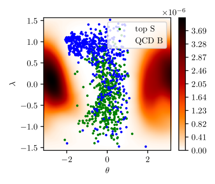
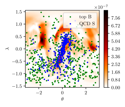
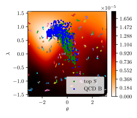
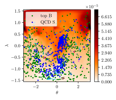
Figure 36: Equirectangular projection of the latent space after pre-training (upper) and after NAE training (lower). The $x$- and $y$-axis are the longitude and latitude on the latent sphere. We train on QCD jets (left) and on top jets (right). The lines represent the path of the LMCs in the current iteration. Figure from Ref. [28].

For the training of the NAE, specifically the estimation of the normalization $Z_{\theta}$ we complement the standard MCMC in phase space with the mapping between latent and phase spaces provided by the autoencoder. If we accept that different initializations of the MCMC defined in Eq.(3.26) lead to different results, we can tune $\lambda_{x}$ and $\sigma_{x}$ in such a way that we can use a sizeable number of short, non-overlapping Markov chains. Next, we apply On-Manifold Initialization (OMI). It is motivated by the observation that sampling the full data space is inefficient due to its high dimensionality, but the training data lies close to a low-dimensional manifold embedded in the data space $x$. All we need to do is to sample close to this manifold. Since we are using an autoencoder this manifold is defined implicitly as the image of the decoder network, meaning that any point in the latent space $z$ passed through the decoder will lie on the manifold. This means we can first focus on the manifold by taking samples from a suitably defined distribution in the low-dimensional latent space, and then map these samples into data space via the decoder. After that, we perform a series of MCMC steps in the full ambient data space to allow the Markov chains to minimize the loss around the manifold. During the OMI it is crucial that we cover the entire latent space, thus a compact latent space is preferable. Just like for the contrastive learning in Sec. 2.4 we normalize the latent vectors so that they lie on the surface of a hypersphere $\mathbb{S}^{D_{z}-1}$, allowing for a uniform sampling of the initial batch in the latent space.

As usual, we apply the NAE to unsupervised top tagging, after training on QCD jets only, and vice versa. For the latent space dimension we use $D_{z}=3$, which allows us to visualize the latent space nicely. Before starting the NAE training we pre-train the network using the standard AE procedure with the standard MSE loss. In the upper panels of Fig. 36 we show a projection of the latent space after training the usual AE. In the left panels we train on the simpler QCD background, which means that the latent space has a simple structure. The QCD jets are distributed widely over the low-energy region, while the anomalous top jets cluster slightly away from the QCD jets. This changes when we train on the more complex top jets, as shown in the right panels. The latent MSE-landscape reflects this complex structure with many minima, and top jets spread over most of the sphere. After the NAE training, only the regions populated by training data have a low MSE. The sampling procedure has shaped the decoder manifold to correctly reconstruct only training jet images. For both training directions, the Markov chains move from a uniform distribution to mostly cover the region with low MSE, leading to an improved separation of the respective backgrounds and signals.

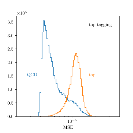
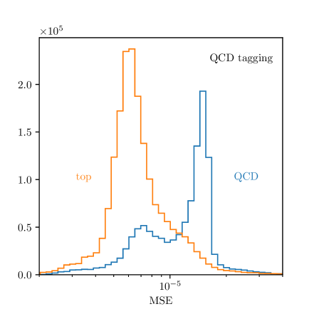
Figure 37: Distribution of the MSE after training on QCD jets (left) and on top jets (right). We show the MSE for QCD jets (blue) and top jets (orange) in both cases. Figure from Ref. [28].

To show how the NAE works symmetrically for anomalous tops and for anomalous QCD jets, we can look at the respective MSE distributions. In the left panel of Fig. 37 we first see the result after training the NAE on QCD jets. The MSE values for the background are peaked strongly, cut off below $4\cdot 10^{-5}$ and with a smooth tail towards larger MSE values. The MSE distribution for top jets is peaked at larger values, and again with an unstructured tail into the QCD region. Alternatively, we see what happens when we train on top jets and search for the simpler QCD jets as an anomaly. In the right panel of Fig. 37 the background MSE is much broader, with a significant tail also towards small MSE values. The QCD distribution develops two distinct peaks, an expected peak in the tail of the top distribution and an additional peak under the top peak. The fact that the NAE manages to push the QCD jets towards larger MSE values indicates that the NAE works beyond the compressibility ordering of the simple AE. However, the second peak shows that a fraction of QCD jets look just like top jets to the NAE.

The success of the NAE shows that anomaly searches at the LHC are possible, but we need to think about the definition of anomalous jets and are naturally lead to phase space densities. This is why we will leave the topic of anomaly searches for now, work on methods for density estimation, and return to the topic in Sec. 5.3.2.

4 Generation and simulation

In the previous chapters we have discussed mainly classification using modern machine learning, using all kinds of supervised and unsupervised training. We have seen how this allows us to extract more complete information and significantly improve LHC analyses. However, classification is not the same as modern analyses in the sense that particle physics analyses have to be related to some kind of fundamental physics question. This means we can either measure a fundamental parameters of the Standard Model Lagrangian, or we can search for physics beyond the Standard Model. Measuring a Wilson coefficient or coupling of the effective field theory version of the Standard Model is the modern way to unify these two approaches. To interpret LHC measurements in such a theory framework the central tool are simulations — how do we get from a Lagrangian to a prediction for observed LHC events in one of the detectors?

Simulations, or event generation based on perturbative QFT is where modern machine learning benefits the theory side of particle physics most. Their input to our simulations is a Lagrangian, from which we can extract Feynman rules, which describe the interactions of the particles we want to produce at the LHC. Using these Feynman rules we then compute the transition amplitudes for the partonic LHC process at a given order in perturbation theory. We have learned how to approximate these amplitudes with NN-surrogates in Sec. 1.2.5. As illustrated in Fig. 2 this includes the production and decays, if we want to separate them, as well as the additional jet radiation from the partons in the initial and final states. Just as the parton splittings forming jets, discussed in Sec. 2.1.1, this part of the simulation is described by the QCD parton splittings. Fragmentation, of the formation and decay of hadrons out of partons is, admittedly, the weak spot of perturbative QCD when it comes to LHC predictions. Finally, we need to describe the detector response through a precision simulation, which is historically in the hands of the experimental collaborations. For theory studies we rely on fast detector simulations, like Delphes, as mentioned in our discussion of the top tagging dataset in Sec. 2.1.3. It turns out that from an ML-perspective event generation and detector simulations are similar tasks, requiring the same kind of generative networks introduced in this section.

The concept which allows us to apply modern machine learning to LHC event generation and simulations is generative networks. To train them, we start with a dataset which implicitly encodes a probability density over a physics or phase space. A generative network learns this underlying density and maps it to a latent space from which we can then sample using for example flat or Gaussian random numbers,

$$r\sim p_{\text{latent}}(r)\quad\to\quad x=f_{\theta}(r)\sim p_{\text{model}}(x)\approx p_{\text{data}}(x)\;.$$ (4.1)

Generative networks allow us to produce samples following a learned distribution. The generated data should then have the same form as the training data, in which case the generative network will produce statistically independent samples reproducing the implicit underlying structures of the training data. Because we train on a distribution of events and there are no labels or any other truth information about the learned phase space density, generative network training is considered unsupervised.

If the network is trained to learn a phase space density, we expect generative networks to require us to compare different distributions, for instance the training distributions $p_{\text{data}}(x)$ and the encoded density $p_{\text{model}}(x)\equiv p_{\text{model}}(x|\theta)$. We already know one way to compare the actual and the modelled phase space density from Eq.(1.11). However, the KL-divergence is only one way to compare such a probability distributions and part of a much bigger field called optimal transport. We remind ourselves of the definition of the KL-divergence,

$$D_{\text{KL}}[p_{\text{data}},p_{\text{model}}]=\Bigg{\langle}\log\frac{p_{\text{data}}(x)}{p_{\text{model}}(x)}\Bigg{\rangle}_{p_{\text{data}}}=\int dx\;p_{\text{data}}(x)\;\log\frac{p_{\text{data}}(x)}{p_{\text{model}}(x)}\;,$$ (4.2)

The KL-divergence between two identical distributions is zero. A disadvantages of this measure is that it is not symmetric, which in the above form means that phase space regions where we do not have data will not contribute to the comparison of the two probability distributions. Two distributions with zero overlap have infinite KL-divergence. If the asymmetric form of the KL-divergence turns out to be a problem, we can easily repair it by introducing the Jensen-Shannon divergence

$$D_{\text{JS}}[p_{\text{data}},p_{\text{model}}] =\frac{1}{2}\left[D_{\text{KL}}\left[p_{\text{data}},\frac{p_{\text{data}}+p_{\text{model}}}{2}\right]+D_{\text{KL}}\left[p_{\text{model}},\frac{p_{\text{data}}+p_{\text{model}}}{2}\right]\right]$$

$$=\frac{1}{2}\left[\int dx\;p_{\text{data}}(x)\;\log\frac{2p_{\text{data}}(x)}{p_{\text{data}}(x)+p_{\text{model}}(x)}+\int dx\;p_{\text{model}}(x)\;\log\frac{2p_{\text{model}}(x)}{p_{\text{data}}(x)+p_{\text{model}}(x)}\right]$$

$$=\frac{1}{2}\int dx\;\left[p_{\text{data}}(x)\;\log\frac{p_{\text{data}}(x)}{p_{\text{data}}(x)+p_{\text{model}}(x)}+p_{\text{model}}(x)\;\log\frac{p_{\text{model}}(x)}{p_{\text{data}}(x)+p_{\text{model}}(x)}\right]+\log 2$$

$$\equiv\frac{1}{2}\Bigg{\langle}\log\frac{p_{\text{data}}(x)}{p_{\text{data}}(x)+p_{\text{model}}(x)}\Bigg{\rangle}_{p_{\text{data}}}+\frac{1}{2}\Bigg{\langle}\log\frac{p_{\text{model}}(x)}{p_{\text{data}}(x)+p_{\text{model}}(x)}\Bigg{\rangle}_{p_{\text{model}}}+\log 2\;.$$ (4.3)

The JS-divergence between two identical distributions also vanishes, but because it samples from both, $p_{\text{data}}$ and $p_{\text{model}}$, it will not explode when the distributions have zero overlap. Instead, we find in this limit

$$D_{\text{JS}}[p_{\text{data}},p_{\text{model}}]\to\frac{1}{2}\int dx\;\left[p_{\text{data}}(x)\;\log\frac{p_{\text{data}}(x)}{p_{\text{data}}(x)}+p_{\text{model}}(x)\;\log\frac{p_{\text{model}}(x)}{p_{\text{model}}(x)}\right]+\log 2=\log 2\;.$$ (4.4)

On thing the KL-divergence and the JS-divergence have in common is that they calculate the difference between two distributions based on the log-ratio of two functional values. Consequently, they reach their maximal values for two distributions with no overlap in $x$, no matter how the two distributions look. This is counter-intuitive, because a distance measure should notice the difference between two identical and two very different distributions with vanishing overlap, for instance a two Gaussians vs a Gaussian and a double-Gaussian. This brings us to the next distance measure, which is meant to work horizontally in the sense that it guarantees for example

$$W[p_{\text{data}}(x),p_{\text{model}}(x)=p_{\text{data}}(x-a)]\approx a\;.$$ (4.5)

This Wasserstein distance or earth mover distance can be most easily defined for weighted sets of points defining each of the two distributions $p_{\text{data}}(x)$ and $p_{\text{model}}(y)$ in a discretized description

$$M_{\text{data}}=\sum_{i=1}^{N_{1}}p_{\text{data},i}\delta_{x_{i}}\qquad\text{and}\qquad M_{\text{model}}=\sum_{j=1}^{N_{2}}p_{\text{model},j}\delta_{y_{j}}\;.$$ (4.6)

We then define a preserving transport strategy as a matrix relating the two sets, namely

$$\pi_{ij}\geq 0\qquad\text{with}\qquad\frac{1}{N_{2}}\sum_{j}\pi_{ij}=p_{\text{data},i}\qquad\frac{1}{N_{1}}\sum_{i}\pi_{ij}=p_{\text{model},j}\;.$$ (4.7)

The first normalization condition ensures that all entries in the model distributions $j$ combined with the data entry $i$ reproduce the full data distribution, the second normalization condition works the other way around. We define the distance between the two represented distributions as

$$W[p_{\text{data}},p_{\text{model}}]=\min_{\pi}\frac{1}{N_{1}N_{2}}\sum_{i,j}|x_{i}-y_{j}|\;\pi_{ij}\;,$$ (4.8)

where the minimum condition implies that we choose the best transport strategy. For our example from Eq.(4.5) with two identical functions this strategy would give $x_{i}-y_{j}=a$. Alternatively, we can write the Wasserstein distance as an expectation value of the distance between two points. This distance has to be sampled over the combined probability distributions and then minimized over the so-called transport plan,

$$W[p_{\text{data}},p_{\text{model}}]=\min\Big{\langle}|x-y|\Big{\rangle}_{p_{\text{data}}(x),p_{\text{model}}(y)}$$ (4.9)

From the algorithmic definition we see that computing the Wasserstein distance is expensive and scales poorly with the number of points in our samples. We will see that these three different distances between distributions can be used for different generative networks, to learn and then sample from an underlying phase space distribution.

4.1 Variational autoencoders

We introduced autoencoders and variational autoencoders already in Sec. 3.2.1, with the idea to map a physics space onto itself with an additional bottleneck (AE) and an induced latent space structure in this bottleneck (VAE). Looking at their network architecture from a generative network point of view, we can also sample from this latent space with corresponding random numbers, for instance with a multi-dimensional Gaussian distribution. In that case the decoder part of the VAE will generate events corresponding to the properties translated from the input phase space to the latent space through the encoder. This means we already know one simple generative model.

In Sec. 3.2.1 we introduced the two-term VAE loss function somewhat ad hoc and without any reference to a probability distribution or a stochastic justification. Let us now tackle it a little more systematically. We start by assuming that we know the data $x$ and its probability distribution $p_{\text{data}}(x)$. This means that given some latent distribution, called $p_{\text{latent}}(r)$ for generative networks, we know the conditional distribution $D(x|r)$ to sample into phase space $x$. To construct this latent distribution, we need the inverse conditional distribution $D(r|x)$. It will eventually define the encoder, and from Bayes’ theorem we know that

$$D(r|x)=\frac{D(x|r)p_{\text{latent}}(r)}{p_{\text{data}}(x)}\;.$$ (4.10)

To construct this encoder and with it the latent representation we resort to the variational approximation, as introduced in Sec. 1.2.4, specifically Eq.(1.39). The goal is to construct a network function $E(r|x)$ which approximates $D(r|x)$ and is controlled by a prior, just like in Eq.(1.39). As before, we construct this approximation using the KL-divergence of Eq.(1.10),

$$D_{\text{KL}}[E(r|x),D(r|x)] =\Bigg{\langle}\log\frac{E(r|x)}{D(r|x)}\Bigg{\rangle}_{E(r|x)}$$

$$=\Bigg{\langle}\log E(r|x)-\log\frac{D(x|r)p_{\text{latent}}(r)}{p_{\text{data}}(x)}\Bigg{\rangle}_{E(r|x)}$$

$$=-\Big{\langle}\log D(x|r)\Big{\rangle}_{E(r|x)}+\Big{\langle}\log E(r|x)-\log p_{\text{latent}}(r)\Big{\rangle}_{E(r|x)}+\log p_{\text{data}}(x)$$

$$=-\Big{\langle}\log D(x|r)\Big{\rangle}_{E(r|x)}+D_{\text{KL}}[E(r|x),p_{\text{latent}}(r)]+\log p_{\text{data}}(x)\;.$$ (4.11)

The evidence $p_{\text{data}}$ is, as before, independent of our network training, which means we can use $D_{\text{KL}}[E(r|x),D(r|x)]$ modulo the last term as the VAE loss function. Also denoting that everything is always evaluated on batches of events from the training dataset we reproduce Eq.(3.9), namely

$$\boxed{\mathcal{L}_{\text{VAE}}=\Big{\langle}-\big{\langle}\log D(x|r)\big{\rangle}_{E(r|x)}+\beta_{\text{KL}}D_{\text{KL}}[E(r|x),p_{\text{latent}}(r)]\Big{\rangle}_{p_{\text{data}}}}\;.$$ (4.12)

We introduce the parameter $\beta_{\text{KL}}$ to allow for a little more flexibility in balancing the two training tasks. Just like the Bayesian network, the VAE loss function derived through the variational approximation includes a KL-divergence as a regularization.

As mentioned above, the structure of the latent space $r$, from which we sample, is introduced by the prior

$$p_{\text{latent}}(r)=\mathcal{N}_{0,1}\;.$$ (4.13)

If we control the $r$-distribution, we can consider the conditional decoder $D(x|r)$ a generative network producing events with the probability we desire. The problem with variational autoencoders in particle physics is that they rely on the assumption that all features in the data can be compressed into a low-dimensional and limited latent space. In the mix of expressivity and achievable precision VAEs are usually not competitive with the other generative network architectures we will discuss next. An exception might be detector simulations, where the underlying physics of calorimeter showers is simple enough to be encoded in a low-dimensional latent space, while the space of detector output channels is huge.

4.2 Generative Adversarial Networks

In our discussion of the VAE we have seen that generative networks are structurally more complex then regression or classification networks. In the language of probability distributions and likelihood losses, we need a generator or decoder network which relies on a conditional probability $E(x|r)$ for the target phase space distribution $x$ given the distribution of the incoming random numbers $r$. For the VAE we used the variational inference trick to construct this latent representation.

An alternative way to learn the underlying density is to combine two networks with adversarial training. Adversarial training means we combine two loss functions

$$\boxed{\mathcal{L}_{\text{adv}}=\mathcal{L}_{1}-\lambda\mathcal{L}_{2}}\;,$$ (4.14)

where the first loss can for example train a classifier and the second term can compute an observable we want to decorrelate. The second network uses the information from the first, classifier network. Because of the negative sign the two sub-networks will now play with each other to find a combined minimum of the loss function. An excellent classifier with small $\mathcal{L}_{1}$ will use and correctly reproduce the to-be-decorrelation variable, implying also a small $\mathcal{L}_{2}$. However, for large enough $\lambda$ the two networks can also work towards a smaller combined loss, where the classifier becomes less ambitious, indicated by a finite $\mathcal{L}_{1}$, but compensated by an even larger $\mathcal{L}_{2}$. This balanced gain works best if the classifier is trained as well as possible, but leaving out precisely the aspects which allow for large values of $\mathcal{L}_{2}$. The two networks playing against each other will then find a compromise where variables entering $\mathcal{L}_{2}$ are ignored in the classifier training represented by $\mathcal{L}_{1}$.

Mathematically, the constructive balance or compromise of two players is called a Nash equilibrium. Varying the coupling $\lambda$ we can strengthen and weaken either of the two sub-networks, a stable Nash equilibrium means that without much tuning of $\lambda$ the two networks settle into a combined minimum. This does not have to be the case, a combination of two networks can of course be unstable in the sense that depending on the size of $\lambda$ either $\mathcal{L}_{1}$ or $\mathcal{L}_{2}$ wins. Another danger in adversarial training is that the adversary network might force the original network to construct nonsense solutions, which we have not thought about, but which formally minimize the combined loss. In the beginning of Sec. 4 we have observed a mechanism which can lead to such poor solution, where the KL-divergence is insensitive to a massive disagreement between data and model, as long as the distribution we sample from in Eq.(4.2) vanishes. In this section we will use adversarial training to construct a generative network.

4.2.1 Architecture

Similar to the VAE structure, the first element of a generative adversarial network (GAN) is the learned generator which replaces the VAE decoder,

$$D(x|r)\Bigg{|}_{p_{\text{latent}}(r)=\mathcal{N}_{0,1}}\quad\longrightarrow\quad G(x|r)\;,$$ (4.15)

where we replace the latent space $r$ with a random number generator $r$ following some simple Gaussian or flat distribution. The argument $x$ is the physical phase space of a jet, a scattering process at the LHC, or a detector output. We remind ourselves that (unweighted) events are nothing but positions in phase space. The difference to the VAE is that we do not train the generator as an inversion or encoder, but use an adversarial loss function like the one shown in Eq.(4.14). The GAN architecture is illustrated in Fig. 38.

Figure 38: Schematic diagram for a GAN. The input $\{r\}$ describes a batch of random numbers, $\{x\}$ denotes a batch of phase space points sampled either from the generator or the training data.

We know from Sec. 2 that it is not hard to train a classification network for jets or events, which means that given a reference dataset $p_{\text{data}}(x)$ and a generated dataset $p_{\text{model}}(x)$ we can train a discriminator or classification network to tell apart the true data and the generated data phase space point by phase space point. This discriminator network is trained to give

$$D(x)=\begin{cases}0&\qquad\text{generated data}\\ 1&\qquad\text{true data}\\ \end{cases}$$ (4.16)

and values in between otherwise. If our discriminator is set up as a proper classification network, its output can be interpreted as the probability of an event being true data. Given a true dataset and a generated dataset, we can train the discriminator to minimize any combination of

$$\big{\langle}1-D(x)\big{\rangle}_{p_{\text{data}}}\qquad\text{and}\qquad\big{\langle}D(x)\big{\rangle}_{p_{\text{model}}}\;.$$ (4.17)

For a perfectly trained discriminator both terms will vanish. On the other hand, we know from Eq.(1.15) that the loss function for such classification task should be the cross entropy, which motivates the discriminator loss

$$\mathcal{L}_{D} =\big{\langle}-\log D(x)\big{\rangle}_{p_{\text{data}}}+\big{\langle}-\log[1-D(x)]\big{\rangle}_{p_{\text{model}}}$$

$$=-\int dx\Big{[}p_{\text{data}}(x)\log D(x)+p_{\text{model}}(x)\log(1-D(x))\Big{]}\;.$$ (4.18)

Comparing this form to the two objectives in Eq.(4.17) we simply enhance the sensitivity by replacing $1-D\to-\log D$. The loss is always positive, and a perfect discriminator will produce zeros for both contributions. From the discriminator loss, we can compute the optimal discriminator output

$$\frac{\delta}{\delta D}\Big{[}p_{\text{data}}(x)\log D+p_{\text{model}}(x)\log(1-D)\Big{]}=\frac{p_{\text{data}}(x)}{D}-\frac{p_{\text{model}}(x)}{1-D} =0$$

$$\Leftrightarrow\qquad D_{\text{opt}}(x)\;p_{\text{model}}(x) =(1-D_{\text{opt}}(x))\;p_{\text{data}}(x)$$

$$\Leftrightarrow\qquad D_{\text{opt}}(x) =\frac{p_{\text{data}}(x)}{p_{\text{data}}(x)+p_{\text{model}}(x)}\;,$$ (4.19)

assuming that the maximum of the integrand also maximizes the integral because of the positive probability distributions.

To train the generator network $G(x|r)$ we now use our adversarial idea. The trained discriminator encodes the agreement of the true and modelled datasets, and all we need to do is evaluate it on the generated dataset

$$\boxed{\mathcal{L}_{G}=\big{\langle}-\log D(x)\big{\rangle}_{p_{\text{model}}}}\;.$$ (4.20)

This loss will vanish when the discriminator (wrongly) identifies all generated events as true events with $D=1$.

In our GAN application this discriminator network gets successively re-trained for a fixed true dataset and evolving generated data. In combination, training the discriminator and generator network based on the losses of Eq.(4.18) and (4.20) in an alternating fashion forms an adversarial problem which the two networks can solve amicably. The Nash equilibrium between the losses implies, just like in Eq.(4.14), that a perfectly trained discriminator cannot tell apart the true and generated samples. To match the literature, we can combine the two GAN losses into one formula by writing them in terms of the generator output $p_{\text{model}}(x)\sim G(r)$ where $r$ follows a random number distribution $p_{\text{latent}}(r)$ as indicated in Eq.(4.15),

$$\mathcal{L}_{D} =\big{\langle}-\log D(x)\big{\rangle}_{p_{\text{data}}}+\big{\langle}-\log[1-D(G(r))]\big{\rangle}_{p_{\text{latent}}}$$

$$\mathcal{L}_{G} =\big{\langle}-\log D(G(r))\big{\rangle}_{p_{\text{latent}}}\;\sim\;\big{\langle}\log[1-D(G(r))]\big{\rangle}_{p_{\text{latent}}}\;.$$ (4.21)

For the generator loss we use the fact that minimizing $-\log D$ is the same as maximizing $\log D$, which is again the same as minimizing $\log(1-D)$ in the range $D\in[0,1]$. The $\sim$ indicates that the two functions will lead to the same result in the minimization, but we will see later that they differ by a finite amount.

After modifying the generator loss we can write the two optimizations for the discriminator and generator training as a min-max game

$$\boxed{\min_{G}\max_{D}\;\big{\langle}\log D(x)\big{\rangle}_{p_{\text{data}}}+\big{\langle}\log[1-D(G(r))]\big{\rangle}_{p_{\text{latent}}}}\;.$$ (4.22)

Finally, we can evaluate the discriminator and generator losses in the limit of the optimally trained discriminator given in Eq.(4.19),

$$\mathcal{L}_{D} \to-\big{\langle}\log D_{\text{opt}}(x)\big{\rangle}_{p_{\text{data}}}-\big{\langle}\log[1-D_{\text{opt}}(x)]\big{\rangle}_{p_{\text{model}}}$$

$$=-\Bigg{\langle}\log\frac{p_{\text{data}}(x)}{p_{\text{data}}(x)+p_{\text{model}}(x)}\Bigg{\rangle}_{p_{\text{data}}}-\Bigg{\langle}\log\frac{p_{\text{model}}(x)}{p_{\text{data}}(x)+p_{\text{model}}(x)}\Bigg{\rangle}_{p_{\text{model}}}$$

$$\equiv-2D_{\text{JS}}[p_{\text{data}},p_{\text{model}}]+2\log 2\;,$$ (4.23)

just inserting the definition in Eq.(4.3). It shows where the GAN will be superior to the KL-divergence-based VAE, because the JS-divergence is more efficient at detecting a mismatch between generated and training data. For the same optimal discriminator the modified generator loss from Eq.(4.21) becomes

$$\mathcal{L}_{G} \to\big{\langle}\log(1-D_{\text{opt}}(x))\big{\rangle}_{p_{\text{model}}}$$

$$=\Bigg{\langle}\log\frac{2p_{\text{model}}(x)}{p_{\text{data}}(x)+p_{\text{model}}(x)}\Bigg{\rangle}_{p_{\text{model}}}-\log 2$$

$$\equiv D_{\text{KL}}\left[p_{\text{model}},\frac{p_{\text{data}}+p_{\text{model}}}{2}\right]-\log 2\;.$$ (4.24)

For a perfectly trained discriminator and generator the Nash equilibrium is given by

$$p_{\text{data}}(x)=p_{\text{model}}(x)\qquad\Rightarrow\qquad\mathcal{L}_{D}=2\log 2\qquad\text{and}\qquad\mathcal{L}_{G}=-\log 2\;$$ (4.25)

We can find the same result from the original definitions of Eq.(4.18) and (4.20), using our correct guess that the perfect discriminator in the Nash equilibrium is constant, namely

$$D(x)=\frac{1}{2}\qquad\Rightarrow\qquad\mathcal{L}_{D} =-\log\frac{1}{2}-\log\frac{1}{2}=2\log 2$$

$$\mathcal{L}_{G} =-\log\frac{1}{2}=\log 2\;.$$ (4.26)

The difference in the value for the generator loss correspond to the respective definitions in Eq.(4.21).

The fact that the GAN training searches for a generator minimum given a trained discriminator, which is different from the generator-alone training, leads to the so-called mode collapse. Starting from the generator loss, we see in Eq.(4.20) that it only depends on the discriminator output evaluated for generated data. This means the generator can happily stick to a small number of images or events which look fine to a poorly trained discriminator. In the discriminator loss in Eq.(4.18) the second term will, by definition, be happy with this generator output as well. From our discussion of the KL-divergence we know that the first term in the discriminator loss will also be fine if large gradients of $\log D(x)$ only appear in regions where the sampling through the training dataset $p_{\text{data}}(x)$ is poor, which means for example unphysical regions.

After noticing that the JS-divergence of the GAN discriminator loss improves over the KL-divergence-base VAE, we can go one step further and use the Wasserstein distance between the distributions $p_{\text{data}}$ and $p_{\text{model}}$. The Wasserstein distance of two non-intersecting distributions grows roughly linearly with their relative distance, leading to a stable gradient. According to the Kantorovich-Rubinstein duality, the Wasserstein distance between the training and generated distributions is given by

$$W(p_{\text{data}},p_{\text{model}})=\max_{D}\left[\big{\langle}D(x)\big{\rangle}_{p_{\text{data}}}-\big{\langle}D(x)\big{\rangle}_{p_{\text{model}}}\right]\;.$$ (4.27)

For the WGAN the discriminator is also called critic. The definition of the Wasserstein distance involves a maximization in discriminator space, so the discriminator has to be trained multiple times for each generator update. A 1-Lipschitz condition can be enforced through a maximum value of the discriminator weights. It can be be replaced by a gradient penalty, as it is used for regular GANs.

4.2.2 Event generation

Figure 39: Schematic diagram for an event-generation GAN. It corresponds to the generic GAN architecture in Fig. 38, but adds the external masses to the input and the MMD loss defined in Eq.(4.32).

As discussed in Sec. 1.1.3, event generation is at the heart of LHC theory. The standard approach is Monte Carlo simulation, as indicated in Fig. 2, and in this section we will describe how it can be supplemented by a generative network. There are several motivations for training a generative network on events: (i) we can use such a network to efficiently encode and ship standard event samples, rather than re-generating them every time a group needs them; (ii) we will see in Sec 4.2.3 that we can typically produce several times as many events using a generative network than used for the training; (iii) understanding generative networks for events allows us to test different ML-aspects which can be used for phase space integration and generation; (iv) we can train generative network flexibly at the parton level or at the jet level; (v) finally, we will describe potential applications in the following sections and use generative networks to construct inverse networks.

The training dataset for event-generation networks are unweighted events, in other words phase space points whose density represents a probability distribution over phase space. One of the standard reference processes is top pair production including decays,

$$pp\to t^{*}\bar{t}^{*}\to(bW^{+*})\;(\bar{b}W^{-*})\to(bu\bar{d})\;(\bar{b}\bar{u}d)$$ (4.28)

The star indicates on-shell intermediate particles, described by a Breit-Wigner propagator and shown in the Feynman diagrams

(120,90) arrow_len2mm curly_len3mm wiggly_len3mm i1,i2 oj11,oj12,ob1,ob2,oj21,oj22 fermion,tension=1.0,width=0.6,label=$q$,lab.side=righti1,vp1 fermion,tension=1.0,width=0.6,label=$\bar{q}$,lab.side=rightvp1,i2 gluon,tension=2.0,width=0.5vp1,vp2 fermion,tension=1.0,width=0.6ob1,vd11 fermion,tension=1.5,width=0.6,label=$t$,lab.side=leftvd11,vp2 fermion,tension=1.5,width=0.6,label=$t$,lab.side=leftvp2,vd21 fermion,tension=1.0,width=0.6vd21,ob2 photon,tension=1.0,width=0.6,label=$W$,lab.side=rightvd11,vd12 photon,tension=1.0,width=0.6,label=$W$,lab.side=leftvd21,vd22 fermion,tension=0.5,width=0.6oj12,vd12,oj11 fermion,tension=0.5,width=0.6oj22,vd22,oj21 $\bar{d}$oj11 $u$oj12 $b$ob1 $b$ob2 $\bar{u}$oj21 $d$oj22                    (130,100) arrow_len2mm curly_len3mm wiggly_len3mm i1,i2 oj11,oj12,ob1,ob2,oj21,oj22 gluon,tension=1.0,width=0.6,label=$g$,lab.side=righti1,vp1 gluon,tension=1.0,width=0.6,label=$g$,lab.side=rightvp2,i2 fermion,tension=0.7,width=0.5vp1,vp2 fermion,tension=1.0,width=0.6ob1,vd11 fermion,tension=1.5,width=0.6,label=$t$,lab.side=leftvd11,vp1 fermion,tension=1.5,width=0.6,label=$t$,lab.side=leftvp2,vd21 fermion,tension=1.0,width=0.6vd21,ob2 photon,tension=1.0,width=0.6,label=$W$,lab.side=rightvd11,vd12 photon,tension=1.0,width=0.6,label=$W$,lab.side=leftvd21,vd22 fermion,tension=0.5,width=0.6oj12,vd12,oj11 fermion,tension=0.5,width=0.6oj22,vd22,oj21 $\bar{d}$oj11 $u$oj12 $X$ob1 $b$ob2 $\bar{u}$oj21 $d$oj22

For intermediate on-shell particles the denominator of the respective propagator is regularized by extending it into the complex plane, with a finite imaginary part [3]

$$\left|\frac{1}{s-m^{2}+im\Gamma}\right|^{2}=\frac{1}{(s-m^{2})^{2}+m^{2}\Gamma^{2}}\;.$$ (4.29)

By cutting the corresponding self-energy diagrams, $\Gamma$ can be related to the decay width of the intermediate particle. In the limit $\Gamma\ll m$ we reproduce the factorization into production rate and branching ratio, combined with the on-shell phase space condition

$$\lim_{\Gamma\to 0}\frac{\Gamma_{\text{part}}}{(s-m^{2})^{2}+m^{2}\Gamma^{2}}=\Gamma_{\text{part}}\;\frac{\pi}{\Gamma}\;\delta(s-m^{2})=\pi\text{BR}_{\text{part}}\;\delta(s-m^{2})$$ (4.30)

For a decay coupling $g$ the width scales like $\Gamma\sim mg^{2}$, so weak-scale electroweak particles have widths in the GeV-range, which means means the Breit-Wigner propagators for top pair production define four sharp features in phase space.

As a first step we ignore additional jet radiation, so the phase space dimensionality of the final state is constant. Each particle in the final state is described by a 4-vector, which means the $t\bar{t}$ phase space has $6\times 4=24$ dimensions. If we are only interested in generating events, we can ignore the detailed kinematics of the initial state, as it will be encoded in the training data. However, we can simplify the phase space because all external particles are on their mass shells and we can compute their energies from their momenta,

$$p^{2}=E^{2}-m^{2}\qquad\Leftrightarrow\qquad E=\sqrt{p^{2}+m^{2}}\;,$$ (4.31)

leaving us with an 18-dimensional phase space and six final-state masses as constant input to the network training. Another possible simplification would be to use transverse momentum conservation combined with the fact that the incoming partons have no momentum in the azimuthal plane. We will now use this additional condition in the network training and instead use it to test the precision of the network. A symmetry we could use is the global azimuthal angle of the process and replacing the azimuthal angles of all final state particle with an azimuthal angle difference to one reference particle.

The main challenge of training a GAN to learn and produce $t\bar{t}$ events is that the Breit-Wigner propagators strongly constrain four of the 18 phase space dimensions, but those directions are hard to extract from a generic parametrization of the final state. To construct the invariant mass of each of the tops the discriminator and generator have to probe a 9-dimensional part of the phase space, where each direction covers several 100 GeV to reproduce a top mass peak with its width $\Gamma_{t}=1.5$ GeV. For a given LHC process and its Feynman diagrams we know which external momenta form a resonance, so we can construct the corresponding invariant mass and give it to the neural network to streamline the comparison between true and generated data. This is much less information than we usually use in Monte Carlo simulations, where we define an efficient phase space mapping from the known masses and widths of every intermediate resonance.

One way to focus the network on a low-dimensional part of the phase space is the maximum mean discrepancy (MMD) combined with a kernel-based method to compare two samples drawn from different distributions. Using one batch of training data points and one batch of generated data points, it computes a distance between the distributions as

$$\text{MMD}^{2}(p_{\text{data}},p_{\text{model}}) =\big{\langle}k(x,x^{\prime})\big{\rangle}_{x,x^{\prime}\sim p_{\text{data}}}+\big{\langle}k(y,y^{\prime})\big{\rangle}_{y,y^{\prime}\sim p_{\text{model}}}-2\big{\langle}k(x,y)\big{\rangle}_{x\sim p_{\text{data}},y\sim p_{\text{model}}}\;,$$ (4.32)

where $k(x,y)$ can be any positive definite, narrow kernel function. Two identical distributions lead to $\text{MMD}(p,p)=0$ given enough statistics. Inversely, if $\text{MMD}(p_{\text{data}},p_{\text{model}})=0$ for randomly sampled batches, the two distributions have to be identical $p_{\text{data}}(x)=p_{\text{model}}(x)$. The shape of the kernels determines how local the comparison between the two distributions is evaluated, for instance though a Gaussian kernel with exponentially suppressed tails or a Breit-Wigner with larger tails. The kernel width becomes a resolution hyperparameter of the combined network. We can include the MMD loss to the generator loss of Eq.(4.20),

$$\mathcal{L}_{G}\to\mathcal{L}_{G}+\lambda_{\text{MMD}}\,\text{MMD}^{2}\;,$$ (4.33)

with a properly chosen coupling $\lambda$, similar to the parton density loss introduced in Sec. 1.2.6. The modified GAN setup for event generation is illustrated in Fig. 39.

To begin with, we can look at relatively flat distributions like energies, transverse momenta, or angular correlations. In Fig. 40 we see that they are learned equally well for final-state and intermediate particles. In the kinematic tails we see that the bin-wise difference of the two distributions increases to around 20%. To understand this effect we estimate the impact of limited training statistics per 1024-event batch through the relative statistical uncertainty on the number of events $N_{\text{tail}}(p_{T})$ in the tail above the quoted $p_{T}$ value. For the $p_{T,b}$-distribution the GAN starts deviating at the 10% level around 150 GeV. Above this value we expect around 25 events per batch, leading to a relative statistical uncertainty of 20%. The top kinematics is slightly harder to reconstruct, leading to a stronger impact from low statistics.

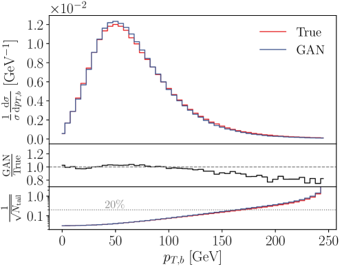
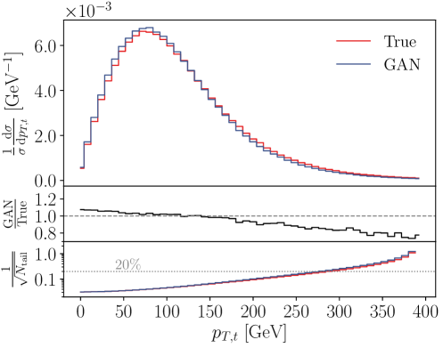
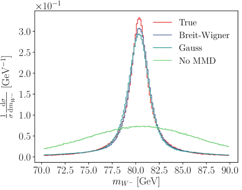
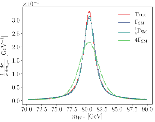
Figure 40: Upper: transverse momentum distributions of the final-state $b$-quark and the decaying top quark for MC truth and the GAN. The lower panels give the bin-wise ratios and the relative statistic uncertainty on the cumulative number of events in the tail of the distribution for our training batch size. Lower: comparison of different kernel functions and varying widths for reconstructing the invariant $W$-mass. Figure from Ref.[29].

Next, we can look at sharply peaked kinematic distributions, specifically the invariant masses which we enhance using the MMD loss. In the lower panels of Fig. 40 we show the effect of the additional MMD loss on learning the invariant $W$-mass distribution. Without the MMD in the loss, the GAN barely learns the correct mass value. Adding the MMD loss with default kernel widths of the Standard Model decay widths drastically improves the results. We can also check the sensitivity on the kernel form and width and find hardly any effect from decreasing the kernel width. Increasing the width reduces the resolution and leads to too broad mass peaks.

In the following sections we will first discuss three aspects of generative networks and statistical limitations in the training data. First, in Sec. 4.2.3 we study how GANs add physics information to a problem similar to a fit to a small number of training data points. Second, in Sec. 4.2.4 we apply generative networks to subtracting event samples, a problem where the statistical uncertainties scales poorly. Third, in Sec. 4.2.5 we use a GAN to unweight events, again a problem where the standard method is known to be extremely inefficient. Finally, in Sec. 4.2.6 we use GANs to enhance the resolution of jet images, again making use of an implicit bias orthogonal to the partonic nature of the jets.

4.2.3 GANplification

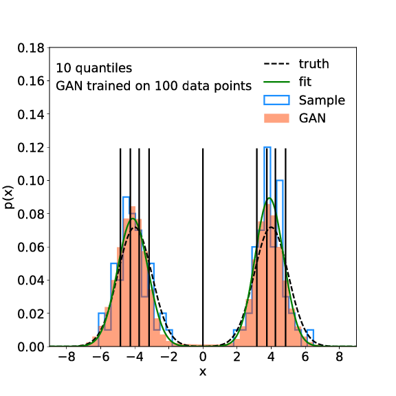
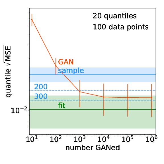
Figure 41: Left: 1-dimensional camel back function, we show the true distribution (black), a histogram with 100 sample points (blue), a fit to the samples data (green), and a high-statistics GAN sample (orange). Right: quantile error for sampling (blue), 5-parameter fit (green), and GAN (orange), shown for 20 quantiles. Figure from Ref. [30].

An interesting question for neural networks in general, and generative networks in particular, is how much physics information the networks include in addition to the information from a statistically limited training sample. For a qualitative answer we can go back to our interpretation of the network as a non-parametric fit. For a fit, nobody would ever ask if a function fitted to a small number of training points can be used to generate a much larger number of points. Also for a network it is clear that the network setup adds information. This is a positive effect of an implicit bias. For neural networks applied to regression tasks we use such an implicit bias, namely that the relevant functions $f(x)$ which we want to approximate are smooth and do not include features below a certain $x$-resolution. Such a smoothness argument also applies to generative networks and the underlying phase space density, the question becomes how much this implicit bias accounts for in terms of events we can generate, compared to the number of training events.

A simple, but instructive toy example is a one-dimensional camel back function, two Gaussians defined by two means, two widths, and a relative normalization, shown in the left panel of Fig. 41. We divide the $x$-axis is into $n_{\text{quant}}$ quantiles, which means that for each bin $j$ we expect the same number of events $\bar{x}_{j}$. To quantify the amount of information in the training data we compute the average quantile error

$$\text{MSE}=\frac{1}{n_{\text{quant}}}\;\sum_{j=1}^{n_{\text{quant}}}\left(x_{j}-\bar{x}_{j}\right)^{2}=\frac{1}{n_{\text{quant}}}\;\sum_{j=1}^{n_{\text{quant}}}\left(x_{j}-\frac{1}{n_{\text{quant}}}\right)^{2}\;,$$ (4.34)

corresponding to the MSE defined in Eq.(1.22). Here $x_{j}$ is the estimated probability for an event to end up in each of the $n_{\text{quant}}$ quantiles, and $\bar{x}_{j}=1/n_{\text{quant}}$ is the constant reference value. In the right panel of Fig. 41 we show this MSE for 100 training points statistically distributed over 20 quantiles. The uncertainty indicated by the shaded region corresponds to the standard deviation from 100 statistically independent sample.

Next, we apply a simple 5-parameter fit to the two means, the two standard deviations, and the relative normalization of the camel back. As expected, the MSE for the fit is much smaller than the MSE for the training data, because the fit function defines a significant implicit bias and is solidly over-constrained by the 100 data points. Again, the error bar corresponds to 100 independent fits. Quantitatively, we find that the fitted function is statistically worth around 500 events instead of the 100-event sample. This means, the fit leads to a statistical amplification by a factor five. If we define an amplification factor for matched MSEs we can write our result as

$$\boxed{A_{\text{fit}}=\frac{N_{\text{sampled}}(\text{MSE}=\text{MSE}_{\text{fit}})}{N_{\text{train}}}\approx 5}\;.$$ (4.35)

Finally, we train a very simple GAN for the 1-dimensional target space on the same 100 data points which we used for the fit. For the first 100 GANned events we find that the MSE corresponds to the 100 training events. This means that the training and generated samples of the same size include the same kind of information. This shows that the properties of the training data are correctly encoded in the network. However, we can use the trained GAN to generate many more events, and in Fig. 41 we see that the MSE improves up to $10^{4}$ events. After that the MSE reaches a plateau and does not benefit from the additional statistics. This curve reflects two effects. First, while the first 100 generated events carry as much information, per event, as the training data, the next 900 events only carry the same amount of information as the next 100 training events. The full information encoded in the network is less than 300 training events, which means additional generated events carry less and less information. Second, the GAN does include roughly as much information as 300 training events, implying an amplification factor

$$A_{\text{GAN}}=\frac{N_{\text{sampled}}(\text{MSE}=\text{MSE}_{\text{GAN}})}{N_{\text{train}}}\approx 3\;,$$ (4.36)

surprisingly close to the parametric fit. This confirms our initial picture of a neural network as a non-parametric fit also for the underlying density learned by a generative network.

This kind of behavior can be observed generally for sparsely populated and high-dimensional phase space, and the amplification factor increases with sparseness. While a quantitative result on achievable amplification factors of generative networks in LHC simulations will depend on many aspects and parameters, this result indicates that using generative networks in LHC simulations can lead to an increase in precision.

4.2.4 Subtraction

The basis of all generative network is that we can encode the density, for instance over phase space, implicitly in a set of events. For particle physics simulations, we can learn the density of a given signal or background process from Monte Carlo simulations, possibly enhanced or augmented by data or in some other way. Most LHC searches include a signal and several background processes, so we have to train a generative network on the combination of background samples. This is not a problem, because the combined samples will describe the sum of the two phase space densities.

The problem becomes more interesting when we instead want to train a generative network to describe the difference of two phase space densities, both given in terms of event samples. There are at least two instances, where subtracting event samples becomes relevant. First, we might want to study signal events based on one sample that includes signal and background and one sample that includes background only. For kinematic distributions many analyses subtract a background distribution from the combined signal plus background distribution. Obviously, this is not possible for individual events, where we have to resort to event weights representing the probability that a given event is signal. Second, in perturbative QCD not all contributions to a cross section prediction are positive. For instance, we need to subtract contributions included in the definition of parton densities from the scattering process in the collinear phase space regions. We also might want to subtract on-shell contributions described by a higher-order simulation code from a more complex but lower-order continuum production, for example in top pair production. In both cases, we need to find a way to train a generative network on two event samples, such that the resulting events follow the difference of their individual phase space densities.

Following the GANplification argument from Sec. 4.2.3, extracting a smooth phase space density for the difference of two samples also has a statistical advantage. If we subtract two samples using histograms we are not only limited in the number of phase space dimensions, we also generate large statistical uncertainties. Let us start with $S+B$ events and subtract $B\gg S$ statistically independent events. The uncertainty on the resulting event number per bin is then

$$\Delta_{S} =\sqrt{\Delta_{S+B}^{2}+\Delta_{B}^{2}}$$

$$=\sqrt{(S+B)+B}\approx\sqrt{2B}\gg\sqrt{S}\;.$$ (4.37)

The hope is that the uncertainty on learned signal density turns out smaller than this statistical uncertainty, because the neural network with its implicit bias constructs smooth distributions for $S+B$ and for $B$ before subtracting them.

Figure 42: Structure of the subtraction GAN. The training data is given by labelled events $\{x_{S,B}\}$ and $\{x_{B}\}$. The label $c$ encodes the category of the generated events. Figure from Ref. [31].

We start with a simple 1-dimensional toy model, i.e.  events which are described by a single real number $x$. We define a combined distribution $p_{S+B}$ and a subtraction distribution $p_{B}$ as

$$p_{S+B}(x)=\frac{1}{x}+0.1\qquad\text{and}\qquad p_{B}(x)=\frac{1}{x}\;.$$ (4.38)

The distribution we want to extract is

$$p_{S}=0.1\;.$$ (4.39)

The subtraction GAN is trained to reproduce the labelled training datasets $\{x_{S+B}\}$ and $\{x_{B}\}$ simultaneously. The architecture is shown in Fig. 42. It consists of one generator and two independent discriminators. The losses for the generator and the two discriminators follow the standard GAN setup in Eq.(4.21). The generator maps random numbers $\{r\}$ to samples $\{x_{G},c\}$, where $x_{G}$ stands for an event and $c=S,B$ for a label. To encode the class label $c$ there are different options. First, we can assign integer values, for instance $c=0$ for background and $c=1$ for signal. The problem with an integer or real label is that the network has to understand this label relative to a background metric. Such a metric will not be symmetric for the two points $c=0,1$. Instead, we can use one-hot encoding by assigning 2-dimensional vectors, just as in Eq.(2.63)

$$c^{\text{one-hot}}_{S}=\begin{pmatrix}1\\ 0\end{pmatrix}\qquad\text{and}\qquad c^{\text{one-hot}}_{B}=\begin{pmatrix}0\\ 1\end{pmatrix}$$ (4.40)

This representation can be generalized to many labels, again without inducing an ordering and breaking the symmetry of the encoding.

In Fig. 42 we see that for the class $\mathcal{C}_{B}$ and the union of $\mathcal{C}_{S}$ with $\mathcal{C}_{B}$ we train two discriminators to distinguish between events from the respective input samples and the labelled generated events. This training forces the events from class $\mathcal{C}_{B}$ to reproduce $p_{B}$ and all events to reproduce $p_{S+B}$. If we then normalize all samples correctly, the events labelled as $\mathcal{C}_{S}$ will follow $p_{S}$. The additional normalization first requires us to assign labels to each event and then to encode them into a counting function based on the one-hot label encoding $I(c)$. This counting function allows us to define a loss term which ensures the correct relative weights of signal and background events,

$$\mathcal{L}_{G}\to\mathcal{L}_{G}+\lambda_{\text{norm}}\left(\dfrac{\sum_{c\in\mathcal{C}_{i}}I(c)}{\sum_{c\in\mathcal{C}_{S+B}}I(c)}-\dfrac{\sigma_{i}}{\sigma_{S+B}}\right)^{2}\;.$$ (4.41)

The individual rates $\sigma_{i}$ are input parameters for example from Monte Carlo simulations.

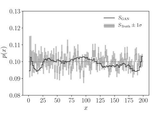
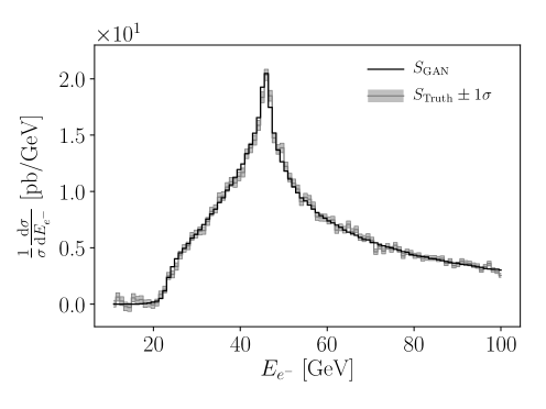
Figure 43: Illustration of the subtraction GAN for 1-dimensional toy events (top) and Drell–Yan events at the LHC. Left: Generated (solid) and true (dashed) events for the two input distributions and the subtracted output. Right: distribution of the subtracted events, true and generated, including the error envelope propagated from the input statistics. Figures from Ref. [31].

In the left panel of Fig. 43 we show the input distributions of Eq.(4.38), as well as the true and generated subtracted distribution. The dotted lines show the training dataset, the full lines show the generated distributions. This comparison confirms that the GAN learns the input information correctly. We also see that the generated subtracted or signal events follow Eq.(4.39). In the right panel we zoom into the subtracted sample to compare the statistical uncertainties from the input data with the generated signal events. The truth uncertainty for the subtracted sample is computed from Eq.(4.37). Indeed, the GAN delivers more stable results than what we expect from the bin-by-bin statistical noise of the training data. The GANned distribution shows systematic deviations, but also at a visibly smaller level than the statistical fluctuation of the input data.

After illustrating ML-subtraction of event samples on a toy model, we need to show how this method works in a particle physics context with 4-momenta of external particles as unweighted events. A simple LHC example is the Drell–Yan process, with a continuum photon contributions and a $Z$-peak. The task is to subtract the photon background from the full process and generate events only for the on-shell $Z$-exchange and the interference with the background,

$$S+B:\qquad pp \to\mu^{+}\mu^{-}$$

$$B:\qquad pp \to\gamma\to\mu^{+}\mu^{-}\;.$$ (4.42)

Aside from the increased dimension of the phase space the subtraction GAN has exactly the same structure as shown in Fig.(42). In the lower panels of Fig. 43 we see how the subtraction clearly extracts the $Z$-mass peak in the lepton energy of the full sample, compared with the feature-less photon continuum in the subtraction sample. The subtracted curve should describe the on-shell $Z$-pole and its interference with the continuum. It vanishes for small lepton energies, where the interference is negligible. In contrast, above the Jacobian peak from the on-shell decay a finite interference remains as a high-energy tail. In the right panel we again show the subtracted curve including the statistical uncertainties from the input samples. Obviously, our subtraction of the background to a di-electron resonance is not a state-of-the-art problem in LHC physics, but it illustrates how neural networks can be used to circumvent conceptual and statistical limitations.

4.2.5 Unweighting

A big technical problem in LHC simulations is how to get from, for example, cross section predictions over phase space to predicted events. Both methods can describe a probability density over phase space, but using different ways of encoding this information:

1. Differential cross sections are usually encoded as values of the probability density for given phase space points. The points themselves follow a distribution, but this distribution has no relevance for the density and only ensures that all features of the distribution are encoded with the required resolution.

2. Events are just phase space points without weights, and the phase space density is encoded in the density of these unweighted events.

Obviously, it is possible to combine these two extreme choices and encode a phase space density using weighted events for which the phase space distribution matters.

If we want to compare simulated with measured data, we typically rely on unweighted events on both sides. There is a standard approach to transform a set of weighted events to a set of unweighted events. Let us consider an integrated cross section of the form

$$\sigma=\int dx\,\frac{d\sigma}{dx}\equiv\int dx\,w(x)\;.$$ (4.43)

The event weight $w(x)$ is equivalent to the probability for a single event $x$. To compute this integral numerically we draw events $\{x\}$ and evaluate the expectation value. If we sample with a flat distribution in $x$ this means

$$\sigma\approx\left\langle\frac{d\sigma}{dx}\right\rangle_{\text{flat}}\equiv\big{\langle}w(x)\big{\rangle}_{\text{flat}}\;.$$ (4.44)

For flat sampling, the information on the cross section is again included in the event weights alone. We can then transform the weighted events $\left\{x,w\right\}$ into unweighted events $\left\{x\right\}$ using a hit-or-miss algorithm. Here, we rescale the weight $w$ into a probability to keep or reject the event $x$,

$$w_{\text{rel}}=\frac{w}{w_{\text{max}}}<1\;,$$ (4.45)

and then use a random number $r\in[0,1]$ such that the event is kept if $w_{\text{rel}}>r$. A shortcoming of this method is that we lose many events, for a given event sample the unweighting efficiency is

$$\epsilon_{\text{uw}}=\frac{\langle w\rangle}{w_{\text{max}}}\ll 1\;.$$ (4.46)

We can improve sampling and integration with a suitable coordinate transformations

$$x\to x^{\prime}\qquad\Rightarrow\qquad\sigma=\int dx\,w(x)=\int dx^{\prime}\,\left|\frac{\partial x}{\partial x^{\prime}}\right|\,w(x^{\prime})\equiv\int dx^{\prime}\;\tilde{w}(x^{\prime})\;.$$ (4.47)

Ideally, the new integrand $\tilde{w}(x^{\prime})$ is nearly constant and the structures in $w(x)$ are fully absorbed by the Jacobian. In this case the unweighting efficiency becomes

$$\tilde{\epsilon}_{\text{uw}}=\frac{\langle\tilde{w}\rangle}{\tilde{w}_{\text{max}}}\approx 1\;.$$ (4.48)

This method of choosing an adequate coordinate transformation is called importance sampling, and the standard tool in particle physics is Vegas.

An alternative approach is to train a generative model to produce unweighted events after training the network on weighted events. We start with the standard GAN setup and loss defined in Eq.(4.21). For weighted training events, the information in the true distribution factorizes into the distribution of sampled events $p_{\text{data}}$ and their weights $w(x)$. To capture this combined information we replace the expectation values from sampling $p_{\text{data}}$ with weighted means,

$$\boxed{\mathcal{L}_{D}=\frac{\big{\langle}-w(x)\,\log D(x)\big{\rangle}_{p_{\text{data}}}}{\langle w(x)\rangle_{p_{\text{data}}}}+\big{\langle}-\,\log[1-D(G(r))]\big{\rangle}_{p_{\text{latent}}}}\;.$$ (4.49)

The generator loss is not affected by this change,

$$\mathcal{L}_{G}=\big{\langle}-\log D(G(r))\big{\rangle}_{p_{\text{latent}}}\;,$$ (4.50)

and because it still produces unweighted events, their weighted means reduce to the standard expectation value of Eq.(4.21).

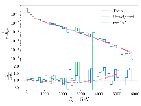
Figure 44: Kinematic distributions for the Drell-Yan process based on 500k weighted training events, 1k unweighted events using standard unweighting, and 30M unweighted events generated with the GAN. Figure from Ref.[32].

As in Sec. 4.2.4, we use weights describing the Drell–Yan process

$$pp\to\mu^{+}\mu^{-}\;,$$ (4.51)

now with a minimal acceptance cut

$$m_{\mu\mu}>50~{}\text{GeV}\;.$$ (4.52)

We can generate weighted events with a naive phase space mapping and then apply the unweighting GAN to those events. For a training dataset of 500k events the weights range from $10^{-30}$ to $10^{-4}$, even if we are willing to ignore more than 0.1% of the generated events. Effects contributing to this vast range are the $Z$-peak, the strongly dropping $p_{T}$-distributions, and our deliberately poor phase space mapping. The classic unweighting efficiency defined by Eq.(4.46) is 0.22%, a high value for state-of-the-art tools applied to LHC processes.

In Fig. 44 we show a set of kinematic distributions, including the deviation from a high-precision truth sample. First, the training dataset describes $E_{\mu}$ all the way to 6 TeV and $m_{\mu\mu}$ beyond 250 GeV with deviations below 5%, albeit with statistical limitation in the low-statistics tail of the $m_{\mu\mu}$ distribution. The sample after hit-and-miss unweighting is limited to 1000 events. Correspondingly, these events only cover $E_{\mu}$ to 1 TeV and $m_{\mu\mu}$ to 110 GeV. In contrast, the unweighting GAN distributions reproduce the truth information, if anything, better than the fluctuating training data. Unlike for most GAN applications, we now see a slight overestimate of the phase space density in the sparsely populated kinematic regions. For illustration purpose we can translate the reduced loss of information into a corresponding size of a hypothetical hit-and-miss training sample, for instance in terms of rate and required event numbers, and find up to an enhancement factor around 100. While it is not clear that an additional GAN-unweighting is the most efficient way of accelerating LHC simulations, it illustrates that generative networks can bridge the gap between unweighted and weighted events. We will further discuss this property for normalizing flow networks in Sec. 4.3.2.

4.2.6 Super-resolution

One of the most exciting applications of modern machine learning in image analysis is super-resolution networks. The simple question is if we can train a network to enhance low-resolution images to higher resolution images, just exploiting general features of the objects in the images. While super-resolution of LHC objects is ill-posed in a deterministic sense, it is well-defined in a statistical sense and therefore completely consistent with the standard analysis techniques at the LHC. Looking at a given analysis object or jet, we would not expect to enhance the information stored in a low-dimensional image by generating a corresponding high-resolution image. However, if we imaging the problem of having to combine two images at different resolution, it should be beneficial to first apply a super-resolution network and then combine the images at high resolution, rather than downsampling the sharper image, losing information, and then combining the two images. Beyond this obvious application, we could ask the question if implicit knowledge embedded in the architecture of the super-resolution network can contribute information in a manner similar as we have seen in Sec. 4.2.3.

Related to the combination of images with different resolution, super-resolution networks will be used in next-generation particle flow algorithms [33]. A related question on the calorimeter level alone is the consistent combination of different calorimeter layers or to ensure an optimal combination of calorimeter and tracking information for charged and neutral aspects of an event. Such approaches are especially promising when both sides of the up-sampling, for instance low-resolution calorimeter data and high-resolution tracking data, are available from data rather than simulations.

We can apply super-resolution to jet images and use the top-tagging dataset described in Sec. 2.1.3 to test the model dependence. The task is then to generate a high-resolution (HR), super-resolved (SR) version of a given low-resolution (LR) image. This kind of question points towards conditional generative networks, which use their sampling functionality to generate events or jets for or under the condition of a fixed event or jet starting point. As before, our QCD and top jet images are generated in the boosted and central kinematic regime with

$$p_{T,j}=550~{}...~{}650~{}\text{GeV}\qquad\text{and}\qquad|\eta_{j}|<2\;,$$ (4.53)

including approximate detector effects. The jet images consist of roughly 50 active pixels, which means a sparsity of 99.8% for $160\times 160$ images. For each jet image we include two representations, one encoding $p_{T}$ in the pixels and one including a power-rescaled $p_{T}^{0.3}$. The first image will efficiently encode the hard pixels, while the second image gains sensitivity for softer pixels especially for QCD jets. This allows the network to cover peaked patterns as well as more global information. The training dataset consists of paired LR/HR images, generated by down-sampling the HR image with down-scaling factors 2, 4, and 8.

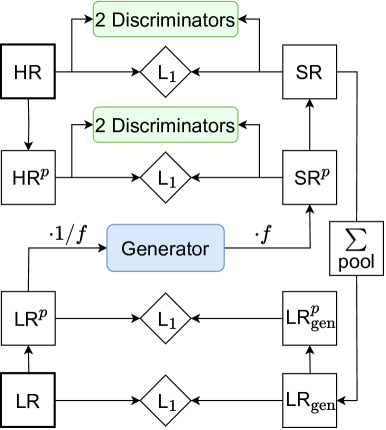
Figure 45: Training process for super-resolution jet images. Figure from Ref. [34].

The main building block of the super-resolution network, illustrated in Fig. 45, is an image generator, following the enhanced super-resolution GAN (ESRGAN) architecture. It converts a LR image into a SR image using a convolutional network. Upsampling a 2-dimensional image works in complete analogy to the downsampling using a convolutional filter, described in Sec. 2.1. For simplicity, let us assume that we want to triple the size of an image using a ($3\times 3$)-filter, which is globally trained. We can then replace every LR-pixel by $3\times 3$ SR pixels multiplying the original pixel with the filter, referred to as a patch. If we want to use the same filter to upsample only by a factor two, we just sum all SR pixel contributions form the LR image. This method is called transposed convolutions, and it can incorporate the same aspects like padding or strides as the regular convolution. An alternative upsampling method is pixel-shuffle. It uses the, in our case 64 feature maps. To double the resolution two dimensions we combine four feature maps and replace each LR pixel with $2\times 2$ SR pixels, one from each feature map. For jet images it turns out that up to three steps with an upsampling factor of two works best if we alternate between pixel-shuffle and transposed convolutions.

The discriminator network is a simple convolutional network. It measures how close the generated SR dataset is to the HR training data and is trained through the usual loss function from Eq.(4.21).

$$\mathcal{L}_{D}=\langle-\log D(x)\rangle_{p_{\text{data}}}+\langle-\log[1-D(G(r))]\rangle_{p_{\text{latent}}}\;.$$ (4.54)

To improve the sensitivity of the discriminator, we also include two versions of it, one trained continuously and one where we erase the memory by resetting all parameters after a certain number of batches.

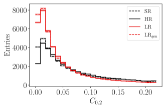
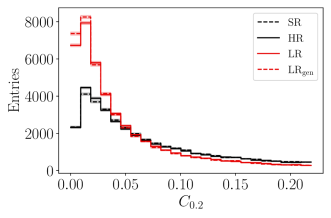
Figure 46: Performance of a super-resolution network trained on QCD jets and applied to QCD jets. We show averaged HR and SR images, average patches for the SR and the HR images, pixel energies, and high-level observables. In the bottom row we show results after training on top jets. Figure from Ref. [34].

The super-resolution generator loss include some additional functionalities. We can start with the usual generator loss from Eq.(4.21). To ensure that the generated SR images and the true HR images really resemble one another, we aid the discriminator by adding a specific term $\mathcal{L}_{\text{HR}}(\text{SR},\text{HR})$ to the generator loss. Similarly, we can downsample the generates SR images and compare this $\text{LR}_{\text{gen}}$ image to the true LR image pixel by pixel. The corresponding contribution to the generator loss is $\mathcal{L}_{\text{LR}}(\text{LR}_{\text{gen}},\text{LR})$. Finally, when upsampling the LR image we need to distribute each LR pixel energy over the appropriate number of SR pixels, a so-called patch. We force the network to spread the LR pixel energy such that the number of active pixels corresponds to the HR truth through the loss contribution $\mathcal{L}_{\text{patch}}(\text{patch(SR)},\,\text{patch(HR)})$, to avoid artifacts. The combined generator loss over the standard and re-weighted jet images is then

$$\boxed{\mathcal{L}_{G}\to\sum_{p=0.3,1}\lambda_{p}\left(\lambda_{\text{HR}}\,\mathcal{L}_{\text{HR}}+\lambda_{\text{LR}}\,\mathcal{L}_{\text{LR}}+\lambda_{G}\,\mathcal{L}_{G}+\lambda_{\text{patch}}\,\mathcal{L}_{\text{patch}}\right)}\;,$$ (4.55)

This loss adds a sizeable number of hyperparameters to the network, which we can tune for example by looking at the set of controlled subjet observables given in Eq.(1.6).

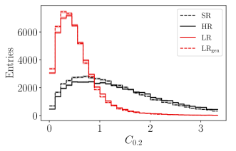
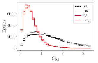
Figure 47: Performance of a super-resolution network trained on top jets and applied to top jets. We show averaged HR and SR images, average patches for the SR and the HR images, pixel energies, and high-level observables. In the bottom row we show results after training on QCD jets. Figure from Ref. [34].

In a first test, we train and test the super-resolution network on QCD jets, characterized by a few central pixels. In Fig. 46 we compare the HR and SR images for QCD jets, as well as the true LR image with their generated $\text{LR}_{\text{gen}}$ counterpart. In addition to average SR and HR images and the relevant patches, we show some pixel energy spectra and high-level observables defined in Eq.(1.6). In the pixel distributions we see how the LR image resolution reaches its limits when, like for QCD jets, the leading pixel carries most of the energy. For the 10th leading pixel we see how the QCD jet largely features soft noise. This transition between hard structures and noise is the weak spot of the SR network. Finally, we show some of the jet substructure observables defined in Eq.(1.6). The jet mass peaks around the expected 50 GeV, for the LR and for the HR-jet alike, and the agreement between LR and $\text{LR}_{\text{gen}}$ on the one hand and between HR and SR on the other is better than the agreement between the LR and HR images. A similar picture emerges for the $p_{T}$-weighted girth $w_{\text{PF}}$, which describes the extension of the hard pixels. The pixel-to-pixel correlation $C_{0.2}$ also shows little deviation between HR and SR on the one hand and LR and $\text{LR}_{\text{gen}}$ on the other.

The situation is different for top jets, which are dominated by two electroweak decay steps. Comparing Figs. 47 with 46 we see that the top jets are much wider and their energy is distributed among more pixels. From a SR point of view, this simplifies the task, because the network can work with more LR-structures. Technically, the original generator loss becomes more important, and we can balance the performance on top-quark jets vs QCD jets using $\lambda_{G}$. Looking at the ordered constituents, the mass drop structure is learned very well. The leading four constituents typically cover the three hard decay sub-jets, and they are described better than in the QCD case. Starting with the 4th constituent, the relative position of the LR and HR peaks changes towards a more QCD-like structure, so the network starts splitting one hard LR-constituent into hard HR-constituents. This is consistent with the top-quark jet consisting of three well-separated patterns, where the QCD jets only show this pattern for one leading constituent. Among the high-level observables, the SR network shifts the jet mass peak by about 10 GeV and does well on the girth $w_{\text{PF}}$, aided by the fact that the jet resolution has hardly any effect on the jet size. As for QCD-jets, $C_{0.2}$ is no challenge for the up-sampling.

The ultimate goal for jet super-resolution is to learn general jet structures, such that SR images can be used to improve multi-jet analyses. In practice, such a network would be trained on any representative jet sample and applied to QCD and top jets the same. This means we need to test the model dependence by training and testing our network on the respective other samples. In the bottom panels of Fig. 46 and 47 we see that this cross-application works almost as well as the consistent training and testing. This means that the way the image pixels are distributed over patches is universal and hardly depends on the partonic nature of the jet.

4.3 Normalizing flows and invertible networks

After discussing the generative VAE and GAN architectures we remind ourselves that controlling networks and uncertainty estimation are really important for regression and classification networks. So the question is if we can apply the recipes from Sec. 1.2.4 to capture statistical or systematic limitations of the training data for generative networks. In LHC applications we would want to know the uncertainties on phase space distributions, for example when we rely on simulations for the background $p_{T}$-distribution in mono-jet searches for dark matter. If we generate large numbers of events, saturating the GANplification effect from Sec. 4.2.3, uncertainties on generated LHC distributions are uncertainties on the precision with which our generative network has learned the underlying phase space distribution it then samples from. There exist, at least, three sources of uncertainty. First, $\sigma_{\text{stat}}(x)$ arises from statistical limitations of the training data. Two additional terms, $\sigma_{\text{sys}}(x)$ and $\sigma_{\text{th}}(x)$ reflect our ignorance of aspects of the training data, which do not decrease when we increase the amount of training data. If we train on data, a systematic uncertainty could come from a poor calibration of particle energy in certain phase space regions. If we train on Monte Carlo, a theory uncertainty will arise from the treatment of large Sudakov logarithms of the kind $\log(E/m)$ for boosted phase space configurations. Once we know these uncertainties as a function of phase space, we can include them in the network output as additional event entries, for instance supplementing

$$\text{ev}=\begin{pmatrix}\{x_{\mu,j}\}\\ \{p_{\mu,j}\}\end{pmatrix}\quad\longrightarrow\quad\begin{pmatrix}\sigma_{\text{stat}}/p\\ \sigma_{\text{syst}}/p\\ \sigma_{\text{th}}/p\\ \{x_{\mu,j}\}\\ \{p_{\mu,j}\}\end{pmatrix}\;,\qquad\text{for each particle $j$.}$$ (4.56)

The first challenge is to extract $\sigma_{\text{stat}}$ without binning, which leads us to introduce normalizing flows directly in the Bayesian setup, in analogy to our first regression network in Secs. 1.2.4 and 1.2.5.

4.3.1 Architecture

To model complex densities precisely and sample from them in a controlled manner, normalizing flows are extremely useful. They transform a random variable

$$r\;\to\;x=G_{\theta}(r)\;,$$ (4.57)

using a bijective mapping. The physical phase space density and the latent density are then related as

$$dx\;p_{\text{model}}(x|\theta) =dr\;p_{\text{latent}}(r)$$

$$\Leftrightarrow \qquad p_{\text{latent}}(r) =p_{\text{model}}(x|\theta)\left|\frac{\partial G_{\theta}(r)}{\partial r}\right|=p_{\text{model}}\big{(}G_{\theta}(r)|\theta\big{)}\left|\frac{\partial G_{\theta}(r)}{\partial r}\right|$$

$$\Leftrightarrow \qquad p_{\text{model}}(x|\theta) =p_{\text{latent}}(r)\left|\frac{\partial G_{\theta}(r)}{\partial r}\right|^{-1}=p_{\text{latent}}\big{(}\overline{G}_{\theta}(x)\big{)}\left|\frac{\partial\overline{G}_{\theta}(x)}{\partial x}\right|$$ (4.58)

where $\overline{G}_{\theta}(x)$ denotes the inverse transformation to $G_{\theta}(r)$ defined in Eq.(4.57). Given a sample $r$ from the latent distribution, we can use $G$ to generate a sample from the target distribution. Alternatively, we can use a sample $x$ from the target distribution to compute its density using the inverse direction. This bijective mapping provides us with a powerful generative pipeline to model the phase space density,

$$\text{latent $r\sim p_{\text{latent}}$}\quad\stackrel{{\scriptstyle[}}{{\leftarrow}}\;\overline{G}_{\theta}(x)]{G_{\theta}(r)\rightarrow}{\xleftrightarrow{\hskip 42.67912pt}}\quad\text{phase space $x\sim p_{\text{data}}$}\;.$$ (4.59)

For this to be a useful approach, we require the latent distribution $p_{\text{latent}}$ to be known and simple enough to allow for efficient sample generation, $G_{\theta}$ to be flexible enough for a non-trivial transformation, and its Jacobian determinant to be efficiently computable. We start by choosing a multivariate Gaussian with mean zero and an identity matrix as the covariance at the distribution $p_{\text{latent}}$ in the unbounded latent space. The INN we will use is a special variant of a normalizing flow network, inspired by the RealNVP architecture, which guarantees a

• bijective mapping between latent space and physics space;

• equally fast evaluation in both direction;

• tractable Jacobian, also in both directions.

The construction of $G_{\theta}$ relies on the usual assumption that a chain of simple invertible nonlinear maps gives us a complex map. This means we transform the latent space into phase space with several transformation layers, for which we need to know the Jacobians. For instance, we can use affine coupling layers as building blocks. Here, the input vector $r$ is split in half, $r=(r_{1},r_{2})$, allowing us to compute the output $x=(x_{1},x_{2})$ of the layer as

$$\begin{pmatrix}x_{1}\\ x_{2}\end{pmatrix}=\begin{pmatrix}r_{1}\odot e^{s_{2}(r_{2})}+t_{2}(r_{2})\\ r_{2}\odot e^{s_{1}(x_{1})}+t_{1}(x_{1})\end{pmatrix}\qquad\Leftrightarrow\qquad\begin{pmatrix}r_{1}\\ r_{2}\end{pmatrix}=\begin{pmatrix}(x_{1}-t_{2}(r_{2}))\odot e^{-s_{2}(r_{2})}\\ (x_{2}-t_{1}(x_{1}))\odot e^{-s_{1}(x_{1})}\end{pmatrix}\;.,$$ (4.60)

where $s_{i},t_{i}$ ($i=1,2$) are arbitrary functions, and $\odot$ is the element-wise product. In practice each of them will be a small multi-layer network. The Jacobian of the transformation $G$ is an upper triangular matrix, and its determinant is just the product of the diagonal entries.

$$\frac{\partial G_{\theta}(r)}{\partial r} =\begin{pmatrix}\partial x_{1}/\partial r_{1}&\partial x_{1}/\partial r_{2}\\ \partial x_{2}/\partial r_{1}&\partial x_{2}/\partial r_{2}\end{pmatrix}=\begin{pmatrix}\text{diag}\left(e^{s_{2}(r_{2})}\right)&\text{finite}\\ 0&\text{diag}\left(e^{s_{1}(x_{1})}\right)\end{pmatrix}$$

$$\qquad\Rightarrow\qquad\left|\frac{\partial G_{\theta}(r)}{\partial r}\right| =\prod e^{s_{2}(r_{2})}\;\prod e^{s_{1}(x_{1})}\;.$$ (4.61)

Such a Jacobian determinant is computationally inexpensive and still allows for complex transformations. We refer to the sequence of coupling layers as $G_{\theta}(r)$, collecting the parameters of the individual nets $s$, $t$ into a joint $\theta$.

Given the invertible architecture we proceed to train our network via a maximum likelihood loss. It relies on the assumption that we have access to a dataset which encodes the intractable phase space distribution $p_{\text{data}}(x)$ and want to fit our model distribution $p_{\text{model}}(x|\theta)$ via $G_{\theta}$. The maximum likelihood loss for the INN is

$$\boxed{\mathcal{L}_{\text{INN}}=-\Big{\langle}\log p_{\text{model}}(x|\theta)\Big{\rangle}_{p_{\text{data}}}=-\Bigg{\langle}\log p_{\text{latent}}\big{(}\overline{G}_{\theta}(x)\big{)}+\log\left|\frac{\partial\overline{G}_{\theta}(x)}{\partial x}\right|\Bigg{\rangle}_{p_{\text{data}}}}\;.$$ (4.62)

The first term ensures that the latent representation remains, for instance, Gaussian, while the second term constructs the correct transformation to the phase space distribution. Given the structure of $\overline{G}_{\theta}(x)$ and the latent distribution $p_{\text{latent}}$, both terms can be computed efficiently. As in Eq.(1.10), one can view this maximum likelihood approach as minimizing the KL-divergence between the true but unknown phase space distribution $p_{\text{data}}(x)$ and our approximating distribution $p_{\text{model}}(x|\theta)$.

While the INN provides us with a powerful generative model of the underlying data distribution, it does not account for an uncertainty in the network parameters $\theta$. However, because of its bijective nature with the known Jacobian, the INN allows us to meaningfully switch from deterministic sub-networks $s_{1,2}$ and $t_{1,2}$ to their Bayesian counterparts. Here we follow exactly the same setup as in Sec. 1.2.4 and recall that we can write the BNN loss function of Eq.(1.44) as

$$\mathcal{L}_{\text{BNN}}=-\Big{\langle}\log p_{\text{model}}(x|\theta)\Big{\rangle}_{\theta\sim q}+D_{\text{KL}}[q(\theta),p(\theta)]\;.$$ (4.63)

We now approximate the intractable posterior $p(\theta|x_{\text{train}})$ with a mean-field Gaussian as the variational posterior $q(\theta)$ and then apply Bayes’ theorem to train the network on the usual ELBO loss, now for event samples

$$\mathcal{L}_{\text{BINN}} =-\Big{\langle}\log p_{\text{model}}(x|\theta)\Big{\rangle}_{\theta\sim q,x\sim p_{\text{data}}}+D_{\text{KL}}[q(\theta),p(\theta)]$$

$$=-\Bigg{\langle}\log p_{\text{latent}}\big{(}\overline{G}_{\theta}(x)\big{)}+\log\left|\frac{\partial\overline{G}_{\theta}(x)}{\partial x}\right|\Bigg{\rangle}_{\theta\sim q,x\sim p_{\text{data}}}+D_{\text{KL}}[q(\theta),p(\theta)]$$ (4.64)

By design, the likelihood, the Jacobian, and the KL-divergence can be computed easily.

To generate events using this model and with statistical uncertainties, we remind ourselves how Bayesian network sample over weight space in Eq.(1.55), but how to predict a phase space density with a local uncertainty map. In terms of the BNN network outputs analogous to Eq.(1.58) this means

$$p(x) =\int d\theta\;q(\theta)\;p_{\text{model}}(x|\theta)$$

$$\sigma_{\text{pred}}^{2}(x) =\int d\theta\;q(\theta)\left[p_{\text{model}}(x|\theta)-p(x)\right]^{2}\;.$$ (4.65)

Here $x$ denotes the initial phase space vector from Eq.(4.56), and the predictive uncertainty can be identified with the corresponding relative statistical uncertainty $\sigma_{\text{stat}}$.

Let us illustrate Bayesian normalizing flows using a set of 2-dimensional toy models. First, we look a simple 2-dimensional ramp distribution, linear in one direction and flat in the other,

$$p(x,y)=2x\;.$$ (4.66)

The factor two ensures that $p(x,y)$ is normalized. The network input and output consist of unweighted events in the 2-dimensional parameters space, $(x,y)$.

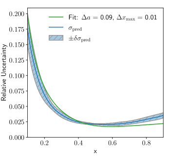
Figure 48: Density and predictive uncertainty distribution for a linear wedge ramp. The uncertainty on $\sigma_{\text{pred}}$ is given by its $y$-variation. The green curve represents a 2-parameter fit to Eq.(4.71). Figure from Ref. [35].

In Fig. 48 we show the network prediction, including the predictive uncertainty on the density. Both, the phase space density and the uncertainty are scalar fields defined over phase space, where the phase space density has to be extracted from the distribution of events and the uncertainty is explicitly given for each event or phase space point. For both fields we can trivially average the flat $y$-distribution. In the left panel we indicate the predictive uncertainty as an error bar around the density estimate, covering the deviation from the true distribution well.

In the central and right panels of Fig. 48 we show the relative and absolute predictive uncertainties. The relative uncertainty decreases towards larger $x$. However, the absolute uncertainty shows a distinctive minimum around $x\approx 0.45$. To understand this minimum we focus on the non-trivial $x$-coordinate with the linear form

$$p(x)=ax+b\qquad\text{with}\qquad x\in[0,1]\;.$$ (4.67)

Because the network learns a density, we can remove $b$ by fixing the normalization,

$$1=\int_{0}^{1}dx(ax+b)=\frac{a^{2}}{2}+b\qquad\Rightarrow\qquad p(x)=a\left(x-\frac{1}{2}\right)+1\;.$$ (4.68)

Let us now assume that the network acts like a one-parameter fit of $a$ to the density, so we can propagate the uncertainty on the density into an uncertainty on $a$,

$$\sigma_{\text{pred}}\equiv\Delta p\approx\left|x-\frac{1}{2}\right|\;\Delta a\;.$$ (4.69)

The absolute value appears because the uncertainties are defined to be positive, as encoded in the usual quadratic error propagation. The minimum at $x=1/2$ explains the pattern we see in Fig. 48. What this simple approximation cannot explain is that the predictive uncertainty is not symmetric and does not reach zero. However. we can modify our simple ansatz to vary the hard-to-model boundaries and find

$$p(x)= ax+b\qquad\text{with}\qquad x\in[x_{\text{min}},x_{\text{max}}]$$

$$\Rightarrow\qquad p(x)= ax+\frac{1-\dfrac{a}{2}(x_{\text{max}}^{2}-x_{\text{min}}^{2})}{x_{\text{max}}-x_{\text{min}}}\;.$$ (4.70)

For the corresponding 3-parameter fit we find

$$\sigma_{\text{pred}}^{2}\equiv(\Delta p)^{2}=\left(x-\frac{1}{2}\right)^{2}(\Delta a)^{2}+\left(1+\frac{a}{2}\right)^{2}(\Delta x_{\text{max}})^{2}+\left(1-\frac{a}{2}\right)^{2}(\Delta x_{\text{min}})^{2}\;.$$ (4.71)

While the slight shift of the minimum is not explained by this form, it does lift the minimum uncertainty to a finite value. If we evaluate the uncertainty as a function of $x$ we cannot separate the effects from the two boundaries. The green line in Fig. 48 gives a 2-parameter fit of $\Delta a$ and $\Delta x_{\text{max}}$ to the $\sigma_{\text{pred}}$ distribution from the Bayesian INN.

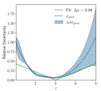
Figure 49: Density and predictive uncertainty distribution for the Gaussian ring. The uncertainty band on $\sigma_{\text{pred}}$ is given by different radial directions. The green curve represents a 2-parameter fit to Eq.(4.74). Figure from Ref. [35].

While the linear ramp example could describe how an INN learns a smoothly falling distribution, like $p_{T}$ of one of the particle in the final state, the more dangerous phase space features are sharp intermediate mass peaks. The corresponding toy model is a 2-dimensional Gaussian ring in terms of polar coordinates,

$$p(r,\phi) =\mathcal{N}_{\mu=4,\sigma=1}(r)\qquad\text{with}\quad\phi\in[0,\pi]$$

$$\Leftrightarrow\qquad p(x,y) =\mathcal{N}_{\mu=4,\sigma=1}(\sqrt{x^{2}+y^{2}})\times\frac{1}{\sqrt{x^{2}+y^{2}}}\;.$$ (4.72)

where the Jacobian $1/r$ ensures that both probability distributions are correctly normalized. We train the Bayesian INN on Cartesian coordinates, just like for the ramp discussed above. In Fig. 49 we show the Cartesian density, evaluated on a line of constant angle. This form includes the Jacobian and leads to a shifted maximum. Again, the uncertainty covers the deviation of the learned from the true density.

Also in Fig. 49 we see that the absolute predictive uncertainty shows a dip at the peak position. As before, this leads us to the interpretation in terms of appropriate fit parameters. For the Gaussian radial density we use the mean $\mu$ and the width $\sigma$, and the corresponding variations of the Cartesian density give us

$$\sigma_{\text{pred}}=\Delta p \supset\left|\dfrac{d}{d\mu}\;p(x,y)\right|\;\Delta\mu$$

$$=\frac{1}{r}\;\frac{1}{\sqrt{2\pi}\sigma}\left|\dfrac{d}{d\mu}\;e^{-(r-\mu)^{2}/(2\sigma^{2})}\right|\;\Delta\mu$$ (4.73)

$$=\frac{p(x,y)}{r}\left|\frac{2(r-\mu)}{2\sigma^{2}}\right|\;\Delta\mu=\frac{p(x,y)}{r}\;\frac{|r-\mu|}{\sigma^{2}}\;\Delta\mu\;.$$ (4.74)

This turns out the dominant uncertainty, and it explains the local minimum at the peak position. Away from the peak, the uncertainty is dominated by the exponential behavior of the Gaussian.

The patterns we observe for the Bayesian INN indicate that our bilinear mapping is constructed very much like a fit. The network first identifies the family of functions which describe the underlying phase space density, and then it adjusts the relevant parameters, like the derivative of a falling function or the peak position of the Gaussian. We emphasize that this result is extracted from a joint network training on the density and the uncertainty on the density, not from a visualization. It also applies to normalizing flows only. Without a tractable Jacobian it is not clear how it can be generalized for example to GANs, even though the results on super-resolution with jets trained on QCD jets and applied to top jets in Fig. 47 suggest that also the GANs first learn general aspects before focusing on details of their model.

4.3.2 Event generation

When we want to use normalizing flows to describe complex phase space distributions we can replace the simple affine coupling layer of Eq.(4.60) with more powerful transformations. One example are splines, smooth rational functions which we typically use for interpolations. Such a spline is spanned by a set of rational polynomials interpolating between a given number of knots. The positions of the knots and the derivatives of the target function at the knots are parameterized by the network as bin widths $\theta_{x}^{j}$, bin heights $\theta_{y}^{j}$, and knot derivatives $\theta_{d}^{j}$, illustrated in Fig. 50.

Figure 50: Visualisation of a spline layer for normalizing flows. The network positions of the spline knots and the derivative at each knot. Splines linking the knots define a monotonic transformation. Figure from Ref. [36].

We already know from Sec. 4.2.5 that it is easy to translate weighted into unweighted event samples through hit-and-miss unweighting. However, we have also seen that this unweighting is computationally expensive, because the range of weights is large. Furthermore, we know from Sec. 4.2.4 that LHC predictions can include events with negative weights, and in this case we cannot easily unweight the sample. What we can do is train a generative model on weighted events, using the modified loss from Eq.(4.62)

$$\boxed{\mathcal{L}_{\text{INN, weighted}}=-\Big{\langle}w(x)\log p_{\text{model}}(x|\theta)\Big{\rangle}_{p_{\text{data}}}}\;.$$ (4.75)

This loss defines the correct optimization of the generative model for all kinds of event samples, including negative weights. Because this loss function only changes the way the network learns the phase space density, the generator will still produce unweighted events.

We postpone the discussion of standard event generation to Sec. 4.3.3, where we also have a look at different sources of uncertainties for generative models. Instead, we will show how normalizing flows can be trained on events with negative weights, specifically the process

$$pp\rightarrow t\bar{t}\;.$$ (4.76)

If we generate events for this process to NLO in QCD, for instance using the Madgraph event generator. For the default setup $23.9\%$ of all events have negative weights.

In Fig. 51 we show two example distributions generated from the unweighting flow-network. The distributions without event weights are to show that the model indeed learns the effect of the events with negative weights. We see that $p_{T,t}$ is essentially unaffected by the weights, because this distribution is already defined by the LO-kinematics, and negative weights only induce to a slight bias for small values of $p_{T,t}$. As always, the generative model runs out of precision in the kinematic tails of the distributions. The picture changes for the $p_{T,tt}$ distribution, which is zero at leading order and only get generated through real-emission corrections, which in turn are described by a mix of positive-weight and negative-weight events. The generative network learns the distribution correctly over the entire phase space. The normalizing flow results in Fig. 51 can be compared to the GANned events in Fig. 40, and we see that the agreement between the normalizing flow and the true phase space density is significantly better than for GANs, which means that normalizing flows are better suited for this kind of precision simulations.

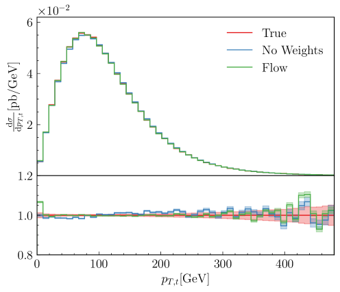
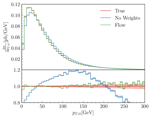
Figure 51: Generated events for $t\bar{t}$ production at NLO, including negative weights. We show the MC truth, the generative normalizing flow, and the MC truth ignoring the sign of the event weights, the latter to illustrate the effects of the negative weights. Figure from Ref. [36].

4.3.3 Control and uncertainties

After confirming that normalizing flows can generate events, let us go back to the Bayesian setup introduced in Sec. 4.3 and analyse a little more systematically how we can extract a controlled and precise prediction from an INN. In Sec. 2.1.4 we have already introduced the strategy we will now follow for precision generative networks. In two steps we first need to control that our network has captured all features of the phase space density and only then can we compute the different uncertainties on the encoded density.

As for most NN-based event generators we now use unweighted LO events as training data, excluding detector effects because they soften sharp phase space features. The production process

$$pp\to Z_{\mu\mu}+\{1,2,3\}~{}\text{jets}$$ (4.77)

is a challenge for generative networks, because it combines a sharp $Z$-resonance with the geometric separation of the jets and a variable phase space dimensions. If we assume that the muons are on-shell, but the jets come with a finite invariant mass, the phase space has $6+n_{\text{jets}}\times 4$ dimensions. Standard cuts for reconstructed jets at the LHC are, as usual

$$p_{T,j}>20~{}\text{GeV}\qquad\qquad\text{and}\qquad\qquad\Delta R_{jj}>0.4\;.$$ (4.78)

In Fig. 52 we show an example correlation between two jets, with the central hole for $\Delta R_{jj}<0.4$. Strictly speaking, such a hole changes the topology of the phase space and leads to a fundamental mismatch between the latent and phase spaces. However, for small holes we can trust the network to interpolate through the hole and then enforce the hole at the generation stage.

Since we have learned that preprocessing will make it easier for our network to learn the phase space density with high precision, we represent each final-state particle by

$$\{\;p_{T},\eta,\Delta\phi,m\;\}\;,$$ (4.79)

where we choose the harder of the two muons as the reference for the azimuthal angle and replace the azimuthal angle difference by $\text{atanh}(\Delta\phi/\pi)$, to create an approximately Gaussian distribution. We then use the jet cuts in Eq.(4.78) to re-define the transverse momenta as $\tilde{p}_{T}=\log(p_{T}-p_{T,\text{min}})$, giving us another approximately Gaussian phase space distribution. Next, we apply a centralization and normalization

$$\tilde{q}_{i}=\frac{q_{i}-\overline{q_{i}}}{\sigma(q_{i})}$$ (4.80)

for all phase space variables $q$. Finally, we would like each phase space variable to be uncorrelated with all other variables, so we apply a linear decorrelation or whitening transformation separately for each jet multiplicity.

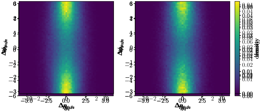
Figure 52: Jet-jet correlations for events with two jets. We show truth (left) and INN-generated events (right). Figure from Ref. [37].

After all of these preprocessing steps, we are left with the challenge of accommodating the variable jet multiplicity. While we will need individual generative networks for each final state multiplicity, we want to keep these networks from having to learning the basic features of their common hard process $pp\to Zj$. Just as for simulating jet radiation, we assume that the kinematics of the hard process depends little on the additional jets. This means our base network gets the one-hot encoded number of jets as condition. Each of the small, additional networks is conditioned on the training observables of the previous networks and on the number of jets. This means we define a likelihood loss for a conditional INN just like Eq.(4.62),

$$p_{\text{model}}(x|\theta)\;\to\;p_{\text{model}}(x|c,\theta)\qquad\Rightarrow\qquad\mathcal{L}_{\text{cINN}} =-\Big{\langle}\log p_{\text{model}}(x|c,\theta)\Big{\rangle}_{p_{\text{data}}}\;,$$ (4.81)

where the vector $c$ includes the conditional jet number, for example. While the three networks for the jet multiplicities are trained separately, they form one generator with a given fraction of $n$-jet events.

To make our INN more expressive with a limited number of layers, we replace the affine coupling blocks of Eq.(4.60) with cubic-spline coupling blocks. The coupling layers are combined with random but fixed rotations to ensure interaction between all input variables. In Fig. 53 we show a set of kinematic distributions from the high-statistics 1-jet process to the more challenging 3-jet process. Without any modification, we see that the $m_{\mu\mu}$ distribution as well as the $\Delta R_{jj}$ distributions require additional work.

One way to systemically improve and control a precision INN-generator is to combine it with a discriminator. This way we can try to exploit different implicit biases of the discriminator and generator to improve our results. The simplest approach is to train the two networks independently and reweight all events with the discriminator output. This only requires that our discriminator output can be transformed into a probabilistic correction, so we train it by minimizing a cross-entropy loss in Eq.(4.21) to extract a probability

$$D(x_{i})\to\begin{cases}0\qquad&\text{generator}\\ 1&\text{truth/data}\end{cases}$$ (4.82)

for each event $x_{i}$. For a perfectly generated sample we should get $D(x_{i})=0.5$. The input to the three discriminators, one for each jet multiplicity, are the kinematic observables given in Eq.(4.79). In addition, we include a set of challenging kinematic correlations, so the discriminator gets the generated and training events in the form

$$x_{i}=\{p_{T,j},\eta_{j},\phi_{j},M_{j}\}\cup\{M_{\mu\mu}\}\cup\{\Delta R_{2,3}\}\cup\{\Delta R_{2,4},\Delta R_{3,4}\}\;.$$ (4.83)

If the the discriminator output has a probabilistic interpretation we can compute an event weight

$$w_{D}(x_{i})=\frac{D(x_{i})}{1-D(x_{i})}\;\to\;\frac{p_{\text{data}}(x_{i})}{p_{\text{model}}(x_{i})}\;.$$ (4.84)

We can see the effect of the additional discriminator in Fig. 53. The deviation from truth is defined through a high-statistics version of the training dataset. The reweighted events are post-processed INN events with the average weight per bin shown in the second panel. While for some of the shown distribution a flat dependence $w_{D}=1$ indicates that the generator has learned to reproduce the training data as well as the discriminator can tell, our more challenging distributions are significantly improved by the discriminator.

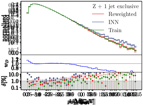
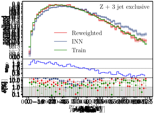
Figure 53: Discriminator-reweighted INN distributions for $Z+$jets production. The bottom panels show the average correction factor obtained from the discriminator output. Figure from Ref. [37].

While the discriminator reweighting provides us with an architecture that learns complex LHC events at the percent level, it comes with the disadvantage of generating weighted events and it does not use the opportunity for the generator and discriminator to improve each other. If it is possible to train the discriminator and generator networks jointly, we could benefit from a GAN-like setup. The problem is that we have not been able to reach the required Nash equilibrium in an adversarial training for the INN generator. As an alternative approach we can include the discriminator information in the appropriately normalized generator loss of Eq.(4.62) through an additional event weight

$$\boxed{\mathcal{L}_{\text{DiscFlow}}=-\Bigg{\langle}w_{D}(x)^{\alpha}\log\frac{p_{\text{model}}(x)}{p_{\text{data}}(x)}\Bigg{\rangle}_{p_{\text{data}}}}\;,$$ (4.85)

in complete analogy to the weighted INN loss in Eq.(4.75). In the limit of a well-trained discriminator this becomes

$$\mathcal{L}_{\text{DiscFlow}} =-\Bigg{\langle}\left(\frac{p_{\text{data}}(x)}{p_{\text{model}}(x)}\right)^{\alpha}\log\frac{p_{\text{model}}(x)}{p_{\text{data}}(x)}\Bigg{\rangle}_{p_{\text{data}}}$$

$$=-\Bigg{\langle}\left(\frac{p_{\text{data}}(x)}{p_{\text{model}}(x)}\right)^{\alpha}\log p_{\text{model}}(x)\Bigg{\rangle}_{p_{\text{data}}}+\Bigg{\langle}\left(\frac{p_{\text{data}}(x)}{p_{\text{model}}(x)}\right)^{\alpha}\log p_{\text{data}}(x)\Bigg{\rangle}_{p_{\text{data}}}\;.$$ (4.86)

Because in our simple DiscFlow setup the discriminator weights $\omega_{D}$ approximating $p_{\text{data}}(x)/p_{\text{model}}(x)$ do not have gradients with respect to the generative model parameters this simplifies to

$$\mathcal{L}_{\text{DiscFlow}} =-\Bigg{\langle}\left(\frac{p_{\text{data}}(x)}{p_{\text{model}}(x)}\right)^{\alpha}\log p_{\text{model}}(x)\Bigg{\rangle}_{p_{\text{data}}}=-\int dx\;\left(\frac{p_{\text{data}}(x)}{p_{\text{model}}(x)}\right)^{\alpha}p_{\text{data}}(x)\;\log p_{\text{model}}(x)\;.$$ (4.87)

The hyperparameter $\alpha$ determines the impact of the discriminator output and can be scheduled. The loss in Eq.(4.87) shows that we are, effectively, training on a shifted reference distribution. If the generator model populates a phase space region too densely, $\omega_{D}<1$ reduces the weight of the training events; if a region is too sparsely populated by the model, $\omega_{D}>1$ amplifies the impact of the training data. As the generator converges to the training data, the discriminator will give $w_{D}(x)\rightarrow 1$, and the generator loss approaches the standard INN form. Unlike the GAN setup from Sec. 4.2 this discriminator–generator coupling does not require a Nash equilibrium between two competing networks.

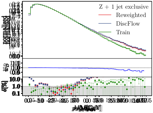
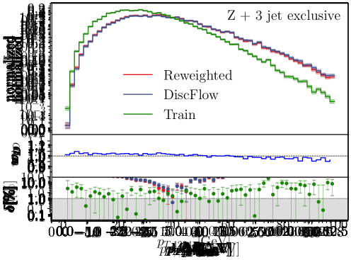
Figure 54: Discriminator-reweighted DiscFlow distributions for $Z+$ jets production. Figure from Ref. [37].

The joint discriminator-generator training has the advantage over the discriminator reweighting that it produces unweighted events. In addition, we can keep training the discriminator after decoupling the generator and reweight the events following Eq.(4.84). In Fig. 54 we show some sample distributions for $Z$+jets production. The DiscFlow generator produces better results than the standard INN generator shown in Fig. 53, but it still benefits from a reweighting postprocessing. For $\Delta R_{jj}<0.4$ we also see that the DiscFlow training only improves the situation in phase space regions where we actually have training data to construct $\omega_{D}(x)$.

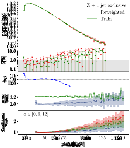
Figure 55: Illustration of uncertainty-controlled INN-generator. We show the reweighted $p_{T,j_{1}}$-distribution for the inclusive $Z$+jets sample, combined with the discriminator $D$, the BINN uncertainty, and the sampled systematic uncertainty defined through the data augmentation of Eq.(4.88). Figure from Ref. [37].

Following our earlier argument, the improved precision of the INN-generator and the control through the discriminator naturally lead us to ask what the uncertainty on the INN prediction is. We already know that the uncertainty estimate from the BNN automatically covers limitations in the training data and training statistics. However, for the generative network we have not discussed systematic uncertainties and data augmentations, like we applied them for instance in Sec. 2.1.4.

In the top panel of Fig. 55 we show the $p_{T,j}$-distribution for $Z+1$ jet production. We choose the simple 2-body final state to maximize the training statistics and the network’s precision. In the second panel we show the relative deviation of the reweighted INN-generator and the training data from the high-statistics truth. While the network does not exactly match the precision of the training data, the two are not far apart, especially in the tails where training statistics becomes an issue. In the third panel we show the discriminator weight $w_{D}$ defined in Eq.(4.84). In the tails of the distribution the generator systematically underestimates the true phase space density, leading to a correction $w_{D}(x)<1$, before in the really poorly covered phase space regions the network predictions starts to fluctuate.

The fourth panel of Fig. 55 shows the uncertainty reported by the Bayesian version of the INN-generator, using the architecture introduced in Sec. 4.3.1. Unlike its deterministic counterpart, the BINN overestimates the phase space density in the poorly populated tail, but the learned uncertainty on the phase space density covers this discrepancy reliably.

Moving on to systematic or theory uncertainties, the problem with generative networks and their unsupervised training is that we do not have access to the true phase space density. The network extracts the density itself, which means that any augmentation, like additional noise, will define either a different density or make the same density harder to learn. One way to include data augmentations is by turning the network training from unsupervised to supervised through an the augmentation by a parameter known to the network. This means we augment our data via a nuisance parameter describing the nature and size of a systematic or theory uncertainty, and train the network conditionally on this parameter. The nuisance parameter is added to the event format given in Eq.(4.56). As a simple example, we can introduce a theory uncertainty proportional to a transverse momentum, inspired by an electroweak Sudakov logarithm. As a function of the parameter $a$ we shift the unit weights of the training events to

$$w=1+a\;\left(\frac{p_{T,j_{1}}-15~{}\text{GeV}}{100~{}\text{GeV}}\right)^{2}\;,$$ (4.88)

where the transverse momentum is given in GeV, we account for a threshold at 15 GeV, and we choose a quadratic scaling to enhance the effects of this augmentation. We train the Bayesian INN conditionally on a set of values $a=0~{}...~{}30$, just extending the conditioning of Eq.(4.81)

$$p_{\text{model}}(x|\theta)\;\to\;p_{\text{model}}(x|a,c,\theta)$$ (4.89)

In the bottom panel of Fig. 55 we show generated distributions for different values of $a$. To incorporate the uncertainty described by the nuisance parameter in the event generation incorporating we sample the $a$-values for example using a standard Gaussian. In combination, we can cover a whole range of statistical, systematic, and theoretical uncertainties by using precise normalizing flows as generative networks. It is not clear if these flows are the final word on LHC simulations and event generation, but for precision simulations they appear to be the leading generative network architecture.

4.3.4 Phase space generation

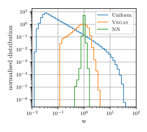
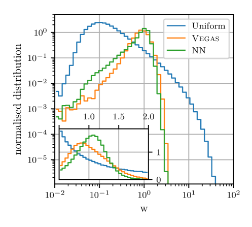
Figure 56: Event weight distributions for sampling the total cross section for $gg\to 3$ jets (left) and 4 jets (right) for $\sqrt{s}=1~{}\text{TeV}$ with $N=10^{6}$ points, comparing Vegas optimization, INN-based optimization and an unoptimized (“Uniform”) distribution. The inset in the right panel shows the peak region on a linear scale. Figure from Ref. [38].

In addition to learning the phase space distribution of events from a set of unweighted events, parton-level events can also be learned from the differential cross section directly. Mathematically speaking, the problem can be formulated as sampling random numbers according to a given functional form. An ML-framework for this is not just useful for LHC event generation, is can be used for any kind of numerical Monte-Carlo integration in high dimensions.

Numerical integration with Monte-Carlo techniques and importance sampling are already discussed in Sec. 4.2.5. Now, we want the coordinate transformation of Eq.(4.47) to be learned by a normalizing flow. In the language of LHC rates of events, we have to transform the differential cross section, $d\sigma$, into a properly normalized distribution,

$$p_{\text{cross section}}=\frac{d\sigma}{\int d\sigma}\;.$$ (4.90)

Then, we can use the loss functions discussed at the beginning of Sec. 4, like the KL-divergence, to learn the distribution. Looking back at Eq.(4.2), we have with the identification of $p_{\text{data}}=p_{\text{cross section}}$

$$\mathcal{L}_{\text{Phase Space}}=D_{\text{KL}}[p_{\text{cross section}},p_{\text{model}}]=\int dx\;p_{\text{cross section}}(x)\;\log\frac{p_{\text{cross section}}(x)}{p_{\text{model}}(x)}\;.$$ (4.91)

The main difference to Eq.(4.2) is that now we do not have training samples from $p_{\text{data}}$, because generating samples according to $p_{\text{cross section}}$ is the problem we want to solve. However, we do have samples distributed according to $p_{\text{model}}$, generated from our model. We can use them for training, provided we correct their weights by introducing a factor $p_{\text{model}}/p_{\text{model}}$ into Eq.(4.91) and then interpreting it as an expectation value over $p_{\text{model}}$,

$$\mathcal{L}_{\text{Phase Space}}=\Bigg{\langle}\frac{p_{\text{cross section}}(x)}{p_{\text{model}}(x)}\log\frac{p_{\text{cross section}}(x)}{p_{\text{model}}(x)}\Bigg{\rangle}_{p_{\text{model}}}\;.$$ (4.92)

However, we have to be careful when computing the gradients of the loss of Eq.(4.92) with respect to the model weights. These enter, in principle, every quantity in Eq.(4.92), namely

• $p_{\text{cross section}}$ in Eq.(4.90) is computed by estimating the integral in the denominator with a Monte-Carlo estimate, which can be improved using importance sampling and samples from $p_{\text{model}}$.

  $$\int d\sigma=\frac{1}{N}\sum d\sigma=\Bigg{\langle}\frac{d\sigma}{p_{\text{model}}}\Bigg{\rangle}_{p_{\text{model}}}\;.$$ (4.93)

  The estimate, however, should just be a constant normalization factor, so the dependence on the network parameters is spurious and a gradient with respect to them will not help the optimization task.

• $p_{\text{model}}$ in the denominator of the prefactor corrects for the fact that we have only samples from the model, not according to $p_{\text{cross section}}$. These can come from the current state of the model, or from a previous one when we recycle previous evaluations. But since this distribution is external to the optimization objective, we should not take gradients of this prefactor.

• $p_{\text{model}}$ in the denominator of the logarithm is the one we want to optimize, so we need its gradient.

The figure of merit, as introduced in Sec. 4.2.5, is the unweighting efficiency. It tells us what fraction of events survives a hit-and-miss unweighting as given in Eq.(4.46). Figure 56 compares the unweighting efficiency for uniformly sampled, Vegas sampled, and INN sampled points in $gg\to 3$ jets and $gg\to 4$ jets. We see that the normalizing flow beats the standard Monte Carlo method by a large margin for the simpler case, but loses its advantage in the right panel. This points to a problem in the scaling of neural network performance with the number of phase space dimensions, as compared to the logarthmic scaling of established Monte Carlo methods.

4.3.5 Calorimeter shower generation

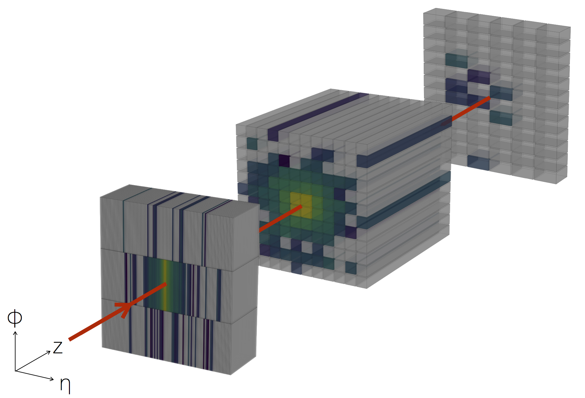
Figure 57: 3-dimensional view of calorimeter shower produced by an incoming $e^{+}$ with $E_{\text{inc}}=10~{}$GeV, simulated with GEANT4. Figure from Ref. [39].

Another application of INNs as generative models in LHC physics is the simulation of the detector response to incoming particles. Such interactions are stochastic and implicitly defines a phase space distribution

$$p(x_{\text{shower}}|\text{initial state})\;.$$ (4.94)

The initial state is characterized by the incoming particle type, energy, position, and angle to the detector surface. For simplicity, we focus on showers originating from the center of the detector volume, and always perpendicular to the surface. We also train a different INN for each particle type, so the learning task is simplified to

$$p(x_{\text{shower}}|E_{\text{inc}})\;.$$ (4.95)

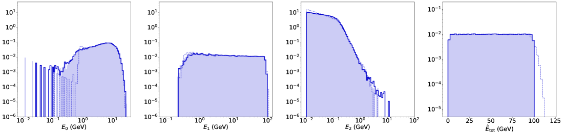
Figure 58: Energy deposition per layer and total energy deposition of $e^{+}$ showers. Figure from Ref. [40].

As ground truth, we use 100,000 showers simulated with GEANT4, a simulation framework based on first principles. Simulating all LHC events with GEANT4 is computationally extremely expensive. Especially high-energy showers can take extremely long to simulate, orders of magnitude longer than low-energy showers due to the larger number of secondary particles needing to be produced and tracked. Whenever only some features of the showers and not all details on energy depositions are needed, fast simulations can be used. In these frameworks, a few high-level features are simulated instead of the full shower information, trading shower fidelity for evaluation speed. Generative networks, such as GANs or INNs, instead allow us to generate showers with many more details in the high-dimensional low-level feature space and with the same speed for all incident energies.

The GANplification effect of Sec. 4.2.3 also applies to calorimeter showers, but there are two more effects that work in our favor and allow us to generate many more events than are in the training sample. The use the fact that calorimeter showers are independent of the hard scattering and independent of each other. Even for a fixed number of training showers the combinatorial factors of combining them with the particles produced in the hard scattering will increase the number of statistically independent events. Second, depending on the chosen voxelization, the generated showers can be rotated before they are combined with an LHC event.

AUC		DNN based classifier
		GEANT4 vs.	GEANT4 vs. (teacher)	GEANT4 vs. (student)
		CaloGAN [39]	CaloFlow v1 [40]	CaloFlow v2 [41]
$e^{+}$	unnorm.	1.000(0)	0.859(10)	0.786(7)
	norm.	1.000(0)	0.870(2)	0.824(4)
$\gamma$	unnorm.	1.000(0)	0.756(48)	0.758(14)
	norm.	1.000(0)	0.796(2)	0.760(3)
$\pi^{+}$	unnorm.	1.000(0)	0.649(3)	0.729(2)
	norm.	1.000(0)	0.755(3)	0.807(1)

Table 4: Classifier-based comparison of calorimeter showers from a GAN, and two autoregressive, flow-based models. Table from Ref. [41].

As an example, we consider $e^{+},\gamma$, and $\pi^{+}$ showers in a simplified version of the ATLAS electromagnetic calorimeter. Showers are digitized into three layers of voxels, with varying size per layer. In total, the dataset contains 504 voxels. The incident energy will be sampled uniformly in $[1,100]$ GeV. Figure 57 shows such a shower. Characteristic for calorimeter datasets, we see a high degree of sparsity and energy depositions ranging over several orders of magnitude. Since the three layers vary in their physical length, the energy deposited on average per layer also differs. To avoid being dominated by the central layer in training, we normalize all showers such that they sum to one in each layer. This normalization can be inverted in the generation when we know the layer energies, so we also have to learn the probability $p(E_{0},E_{1},E_{2}|E_{\text{inc}})$. This can either be done by an independent generative model, or by augmenting the normalized voxel energies with the layer energy information.

When training normalizing flows for calorimeter showers, the high degree of sparsity tends to overwhelm the likelihood loss. The network focuses on learning the many zero entries and does not do well on single voxels with the dominant energy depositions. To ameliorate this, we add noise below the read-out threshold of the detector to the voxels. After generation, we then remove all entries below that threshold and recover the correct sparsity. In Fig. 58 we show the deposited energies in the three layers and overall, for $e^{+}$ showers from GEANT4, a GAN, and a normalizing flow.

The main advantage of generative models over GEANT4 is speed. The first flow-based approach, however, was based on an autoregressive architecture, which is fast to train but a factor 500 (given by the dimensionality of the voxel space) slower in generation. This means that for a batch size of 10k showers, a GPU can produce a single shower in 36ms. Even though this is significantly faster than GEANT4 (1772ms), it is much slower than the GAN (0.07ms). This difference can be addressed in two ways. One would be to use an alternative normalizing flow architecture. The second one is to train a second autoregressive flow with the inverse speed preference: fast sample generation and slow evaluation of the likelihood loss. We can then avoid this training so-called probability density distillation, or teacher-student training. Starting from a flow trained with the likelihood loss (CaloFlow v1), we freeze its weights and train a second flow to match the output of the first flow. Using an MSE loss after every transformation and also to match the output of each of the NNs, we ensure that this new flow becomes a copy of the first one, but with a fast generative direction.

To judge the quality of the generated showers in full phase space, we can train a classifier to distinguish generated showers from GEANT4 showers. Invoking the Neyman–Pearson lemma from Sec. 1.2.1 we conclude that $p_{\text{model}}=p_{\text{data}}$ if the classifier is confused after training. Table 4 shows the AUC of such classifier trainings. First, we see that the GAN, in spite of its in-house classifiers does not provide precise copies of the training showers. The comparison between the student and teacher networks in the dual-flow ansatz shows no clear preference.

5 Inverse problems and inference

If we use our simulation chain in Fig. 2 in the forward direction, the typical LHC analysis starts with a new, theory-inspired hypothesis encoded in a Lagrangian as new particles and couplings. For every point in the BSM parameter space we simulate events, compare them to the measured data using likelihood methods, and discard the BSM physics hypothesis. This approach is inefficient for a variety of reasons:

1. BSM physics hypotheses have free model parameters like masses or couplings, even if an analysis happens to be independent of them. If the predicted event rates follow a simple scaling, like for a truncated effective theory, this is simple, but usually we need to simulate events for each point in model space.

2. There is a limit in electroweak or QCD precision to which we can reasonably include predictions in our standard simulation tools. Beyond this limit we can, for instance, only compute a limited set of kinematic distributions, which excludes these precision prediction from standard analyses.

3. Without a major effort it is impossible for model builders to derive competitive limits on a new model by recasting an existing analysis, if the analysis requires the full experimental and theoretical simulation chains.

These three shortcomings point to the same task: we need to invert the simulation chain, apply this inversion to the measured data, and compare hypotheses at the level of the hard scattering. Detector unfolding is a known, but non-standard application. For hadronization and fragmentation an approximate inversion is standard in that we always apply jet algorithms to extract simple parton properties from the complex QCD jets. Removing QCD jets from the hard process is a standard task in any analysis using jets for the hard process and leads to nasty combinatorial backgrounds. Unfolding to parton level is being applied in top physics, assuming that the top decays are correctly described by the Standard Model. Finally, unfolding all the way to the parton-level is called the matrix element method and has been applied to Tevatron signatures, for example single top production. All of these inverse simulation tasks have been tackled with classical methods, and we will see how the can benefit from modern neutral networks.

Inverse problems in particle physics can be illustrated most easily for the case of detector effects. As a one-dimensional binned toy example we look at a parton-level distribution $f_{\text{parton},j}$ which gets transformed into $f_{\text{reco},j}$ at detector or reconstruction level. We can model these detector effects as part of the forward simulation through the kernel or response matrix $G_{ij}$,

$$f_{\text{reco},i}=\sum_{j=1}^{N}G_{ij}\;f_{\text{parton},j}\;.$$ (5.1)

We postulate the existence of an inversion with the kernel $\overline{G}$ through the relation

$$f_{\text{parton},k}=\sum_{i=1}^{N}\overline{G}_{ki}f_{\text{reco},i}=\sum_{j=1}^{N}\left(\sum_{i=1}^{N}\overline{G}_{ki}G_{ij}\right)f_{\text{parton},j}\quad\text{with}\quad\sum_{i=1}^{N}\overline{G}_{ki}G_{ij}=\delta_{kj}\;.$$ (5.2)

If we assume that we know the $N^{2}$ entries of the kernel $G$, this form gives us the $N^{2}$ conditions to compute its inverse $\overline{G}$. We illustrate this one-dimensional binned case with a toy-smearing matrix

$$G =\begin{pmatrix}1-x&x&0\\ x&1-2x&x\\ 0&x&1-x\end{pmatrix}\;.$$ (5.3)

We can assume $x\ll 1$, but we do not have to. We look at two input vectors, keeping in mind that in an unfolding problem we typically only have one kinematic distribution to determine the inverse matrix $\overline{G}$,

$$f_{\text{parton}} =n\begin{pmatrix}1\\ 1\\ 1\end{pmatrix} \Rightarrow\quad f_{\text{reco}}=f_{\text{parton}}\;,$$

$$f_{\text{parton}} =\begin{pmatrix}1\\ n\\ 0\end{pmatrix} \Rightarrow\quad f_{\text{reco}}=f_{\text{parton}}+x\begin{pmatrix}n-1\\ -2n+1\\ n\end{pmatrix}\;.$$ (5.4)

The first example shows how for a symmetric smearing matrix a flat distribution removes all information about the detector effects. This implies that we might end up with a choice of reference process and phase space such that we cannot extract the detector effects from the available data. The second example illustrates that for bin migration from a dominant peak the information from the original $f_{\text{parton}}$ gets overwhelmed easily. We can also compute the inverse of the smearing matrix in Eq.(5.3) and find

$$\overline{G}\approx\frac{1}{1-4x}\begin{pmatrix}1-3x&-x&x^{2}\\ -x&1-2x&-x\\ x^{2}&-x&1-3x\end{pmatrix}\;,$$ (5.5)

where we neglect the sub-leading $x^{2}$-terms whenever there is a linear term as well. The unfolding matrix extends beyond the nearest neighbor bins, which means that local detector effects lead to a global unfolding matrix and unfolding only works well if we understand our entire dataset. The reliance on useful kinematic distributions and the global dependence of the unfolding define the main challenges once we attempt to unfold the full phase space of an LHC process.

Current unfolding methods follow essentially this simple approach and face three challenges. First, the required binning into histograms is chosen before the analysis and ad-hoc, so it is not optimal. Second, the matrix structure behind correlated observables implies that we can only unfold two or three observables simultaneously. Finally, detector unfolding often misses some features which affect the detector response.

5.1 Inversion by reweighting

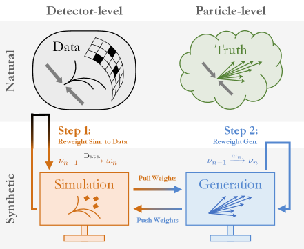
Figure 59: Illustration of the Omnifold method for detector unfolding. Figure from Ref. [42].

OmniFold is an ML-based techniques which iteratively unfolds detector effects. It works on high-dimensional phase spaces and does not require histograms or binning. Its reweighting technique is illustrated in Fig. 59. The goal is to start from reconstruction-level data and predict the parton-level configuration for a measured configuration. It avoids a direct mapping from reconstruction-level to parton level and instead employs an iterative reweighting based on simulated pairs of parton-level and reconstruction-level configurations,

$$(x_{\text{parton}},x_{\text{reco}})\;.$$ (5.6)

As a starting point, we assume that the simulated events have finite weights, while the data starts with unit weights,

$$\nu_{0}(x_{\text{parton}})=\nu_{0}(x_{\text{reco}})\Bigg{|}_{\text{model}}\qquad\text{and}\qquad\omega_{0}(x_{\text{reco}})\Bigg{|}_{\text{data}}=1\;.$$ (5.7)

The Omnifold algorithm consists of four steps:

1. First, it reweights the simulated reconstruction-level events to match the measured reconstruction-level events. The weight $\omega_{1}$ is given by the factor we need to apply to the events $x_{\text{reco}}$, initially following $p_{\text{model}}(x_{\text{reco}},\nu_{0})$, to reproduce $p_{\text{data}}(x_{\text{reco}},1)$,

   $$\frac{\omega_{1}(x_{\text{reco}})}{\nu_{0}(x_{\text{reco}})}=\frac{p_{\text{data}}(x_{\text{reco}},1)}{p_{\text{model}}(x_{\text{reco}},\nu_{0})}\;.$$ (5.8)

   We include the weights as an explicit argument of the likelihoods. In practice, $\omega_{1}$ is extracted from a classification network encoding the likelihood ratio

2. Then, it uses the paired simulation to transfer (pull) this weight to the corresponding parton-level event,

   $$\omega_{1}(x_{\text{reco}})\;\to\;\omega_{1}(x_{\text{parton}})\;.$$ (5.9)

3. Also at the parton level we have a phase space distribution we want to reproduce. This introduces a weight $\nu_{1}$, extracted through another likelihood ratio

   $$\frac{\nu_{1}(x_{\text{parton}})}{\nu_{0}(x_{\text{parton}})}=\frac{p_{\text{model}}(x_{\text{parton}},\omega_{1})}{p_{\text{model}}(x_{\text{parton}},\nu_{0})}\;.$$ (5.10)

4. This new weight we transfer back (push) to the reconstruction level,

   $$\nu_{1}(x_{\text{parton}})\;\to\;\nu_{1}(x_{\text{reco}})\;.$$ (5.11)

   We then go back to Eq.(5.8) and re-iterate the two steps until all likelihood ratios become unity.

Once the Omnifold algorithm converges, the phase space distribution at the parton level is given by

$$p_{\text{unfold}}(x_{\text{parton}})=\nu_{\infty}(x_{\text{parton}})\;p_{\text{model}}(x_{\text{parton}})\;.$$ (5.12)

Because this method does not require any simulations and works on fixed, paired datasets, it is fast and efficient. The ultimate question is how well it describes correlations between phase space points.

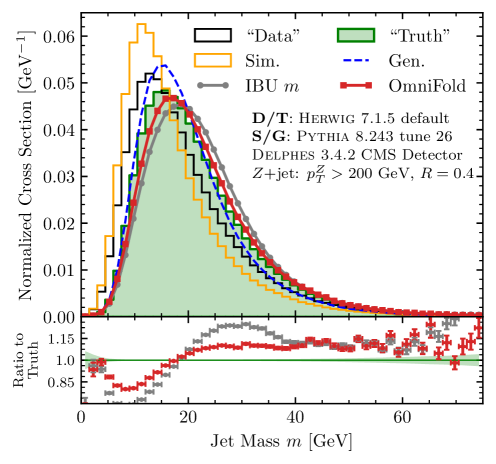
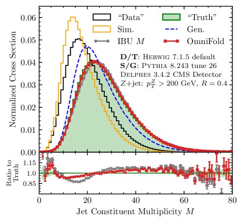
Figure 60: Unfolding results for sample substructure observables, using Herwig jets as data and using Pythia for the simulation. The lower panels include statistical uncertainties on the 1-dimensional distributions. The jet multiplicity $M$ corresponds to $n_{\text{PF}}$ defined in Eq.(1.6). Figure from Ref. [42].

To illustrate the performance of Omnifold, we look at jets and represent the actual data, $p_{\text{data}}(x_{\text{reco}})$, with the Herwig event generator. For the simulation of paired jets, $p_{\text{model}}(x_{\text{parton}})$ and $p_{\text{model}}(x_{\text{parton}})$, we use the Pythia event generator. We then use Omnifold can unfold the Herwig data to the parton level, and compare these results with the true Herwig distributions at the parton level

$$p_{\text{unfold}}(x_{\text{parton}})\;\leftrightarrow\;p_{\text{data}}(x_{\text{parton}})\;.$$ (5.13)

While the event information can be fed into the network in many ways, the Omnifold authors choose to use the deep sets representation of point clouds as introduced in Sec. 2.3.4. For a quantitative test we show set of jet substructure observables, defined in Eq.(1.6). The detector effects, described by the fast Delphes simulation can we seen in the difference between the generation curves, $p_{\text{model}}(x_{\text{parton}})$, and the simulation curves, $p_{\text{model}}(x_{\text{reco}})$. We see that the jet mass and the constituent multiplicity are significantly reduced by the detector resolution and thresholds. The data distributions from Herwig represent $p_{\text{data}}(x_{\text{reco}})$, and we observe a significant difference to the simulation, where Herwig jets have more constituents than Pythia jets.

If we now use the Pythia-trained Omnifold algorithm to unfold the mock data we can compare the results to the green truth curves. The ratio $p_{\text{unfold}}(x_{\text{parton}})/p_{\text{data}}(x_{\text{parton}})$ is shown in the lower panels. We see that, as any network, this deviation is systematic in the bulk and becomes noisy in the kinematic tails. The same is true for the classical, bin-wise iterative Bayesian unfolding (IBU), and the unbinned and multi-dimensional Omnifold method clearly beats the bin-wise method.

5.2 Conditional generative networks

Instead of constructing a backwards mapping for instance from the detector level to the parton level using classifier reweighting, we can also tackle this inverse problem with generative networks, specifically a conditional normalizing flow or cINN. In this section we will describe two applications of this versatile network architecture, one for unfolding and one for inference or measuring model parameters.

5.2.1 cINN unfolding

The idea of using conditional generative networks for unfolding is to generalize the binned distributions Eq.(5.1) to a continuous description of the entire respective phase spaces,

$$\frac{d\sigma}{dx_{\text{reco}}}=\int dx_{\text{parton}}\;G(x_{\text{reco}},x_{\text{parton}})\;\frac{d\sigma}{dx_{\text{parton}}}\;.$$ (5.14)

To invert the detector simulation we define a second transfer function $\overline{G}$ in analogy to Eq.(5.2),

$$\frac{d\sigma}{dx_{\text{parton}}} =\int dx_{\text{reco}}\;\overline{G}(x_{\text{parton}},x_{\text{reco}})\;\frac{d\sigma}{dx_{\text{reco}}}$$

$$=\int dx_{\text{parton}}^{\prime}\;\frac{d\sigma}{dx_{\text{parton}}^{\prime}}\int dx_{\text{reco}}\;\overline{G}(x_{\text{parton}},x_{\text{reco}})G(x_{\text{reco}},x_{\text{parton}}^{\prime})\;.$$ (5.15)

This inversion is fulfilled if

$$\int dx_{\text{reco}}\;\overline{G}(x_{\text{parton}},x_{\text{reco}})G(x_{\text{reco}},x_{\text{parton}}^{\prime})=\delta(x_{\text{parton}}-x_{\text{parton}}^{\prime})\;,$$ (5.16)

all in complete analogy to the binned form above. The symmetric form of Eq.(5.14) and Eq.(5.15) indicates that $G$ and $\overline{G}$ are both defined as distributions for suitable test functions.

Both directions, the forward simulation and the backward unfolding, are stochastic in nature. Based on the statistical picture we should switch from joint probabilities to conditional probabilities using Bayes’ theorem. The forward detector simulation is then described by $G(x_{\text{reco}}|x_{\text{parton}})$, whereas $\overline{G}(x_{\text{parton}}|x_{\text{reco}})$ gives the probability of the model $x_{\text{parton}}$ being true given the observation $x_{\text{reco}}$. Instead of Eq.(5.16) we now have to employ Bayes’ theorem to relate the two directions

$$\overline{G}(x_{\text{parton}}|x_{\text{reco}})=\frac{G(x_{\text{reco}}|x_{\text{parton}})\;p(x_{\text{parton}})}{p(x_{\text{reco}})}\;,$$ (5.17)

where $G$ and $\overline{G}$ now denote conditional probabilities. For the inverse direction we can consider $p(x_{\text{reco}})$ the evidence and ignore it as part of the normalization, but $p(x_{\text{parton}})$ remains as a model dependence for instance through the choice training data. From a physics perspective, it makes sense to assume that detector simulations are at least approximately independent of the hard process, so the inverse simulation should be well defined at the statistical level. If the inversion shows an unwanted model dependence, we can follow a reweighting strategy similar to the one described in Sec. 5.1 to define model-independent training datasets.

Figure 61: Illustration of the cINN setup. Figure from Ref. [43].

For the generative task we employ an INN to map an set of random numbers to a parton-level phase space with the corresponding dimensionality. To capture the information from the reconstruction-level events we condition the INN on such an event. Trained on a given process the network will now generate probability distributions for parton-level configurations given a reconstruction-level event and an unfolding model. The cINN is still invertible in the sense that it includes a bi-directional training from Gaussian random numbers to parton-level events and back, but the invertible nature is not what we use to invert the detector simulation. We will eventually need show how the conditional INN retains a proper statistical notion of the inversion to parton level phase space. This avoids a major weakness of standard unfolding methods, namely that they only work on large enough event samples condensed to one-dimensional or two-dimensional kinematic distributions, such as a missing transverse energy distribution in mono-jet searches or the rapidities and transverse momenta in top pair production.

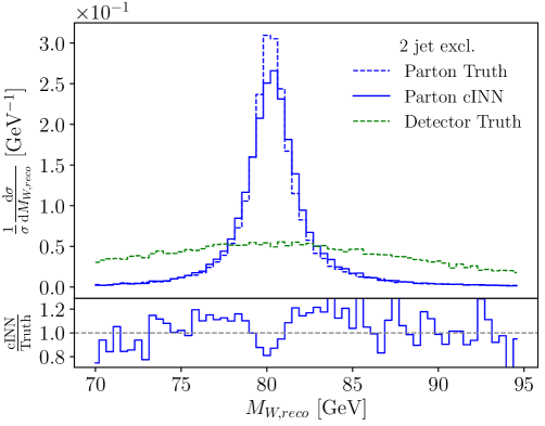
Figure 62: cINNed $p_{T,q}$ distributions. Training and testing events include exactly two jets. The lower panels give the ratio of cINNed to parton-level truth. Figure from Ref. [43].

The structure of the conditional INN (cINN) is illustrated in Fig. 61. We first preprocess the reconstruction-level data by a small subnet, $x_{\text{reco}}\to f(x_{\text{reco}})$ and omit this additional step below. After this preprocessing, the detector information is passed to the functions $s_{i}$ and $t_{i}$ in Eq.(4.60), which now depend on the input, the output, and on the fixed condition. The cINN is trained a loss similar to Eq.(4.62), but now maximizing the probability distribution for the network weights $\theta$, conditional on $x_{\text{parton}}$ and $x_{\text{reco}}$ always sampled in pairs

$$\boxed{\mathcal{L}_{\text{cINN}}=-\Big{\langle}\log p_{\text{model}}(\theta|x_{\text{parton}},x_{\text{reco}})\Big{\rangle}_{p_{\text{parton}}\sim p_{\text{reco}}}}\;.$$ (5.18)

Next, we need to turn the posterior for the network parameters into a likelihood for the network parameters and evaluate the probability distribution for the event configurations. Because we sample the parton-level and reconstruction-level events as pairs, it does not matter which of the two we consider for the probability. We use Bayes’ theorem to turn the probability for $\theta$ into a likelihood, with $x_{\text{parton}}$ as the argument,

$$\mathcal{L}_{\text{cINN}} =-\Bigg{\langle}\log\frac{p_{\text{model}}(x_{\text{parton}}|x_{\text{reco}},\theta)p_{\text{model}}(\theta|x_{\text{reco}})}{p_{\text{model}}(x_{\text{parton}}|x_{\text{reco}})}\Bigg{\rangle}_{p_{\text{parton}}\sim p_{\text{reco}}}$$

$$=-\Big{\langle}\log p_{\text{model}}(x_{\text{parton}}|x_{\text{reco}},\theta)\Big{\rangle}_{p_{\text{parton}}\sim p_{\text{reco}}}-\log p_{\text{model}}(\theta)+\text{const}\;.$$ (5.19)

As before, we ignore all terms irrelevant for the minimization. The second term is a simple weight regularization, which we also drop in the following. We now apply the usual coordinate transformation, defined in Fig. 61, to introduce the trainable Jacobian,

$$\mathcal{L}_{\text{cINN}} =-\Big{\langle}\log p_{\text{model}}(x_{\text{parton}}|x_{\text{reco}},\theta)\Big{\rangle}_{p_{\text{parton}}\sim p_{\text{reco}}}$$

$$=-\Bigg{\langle}\log p_{\text{latent}}(\overline{G}_{\theta}(x_{\text{parton}}|x_{\text{reco}}))+\log\left|\frac{\partial\overline{G}_{\theta}(x_{\text{parton}}|x_{\text{reco}})}{\partial x_{\text{parton}}}\right|\Bigg{\rangle}_{p_{\text{parton}}\sim p_{\text{reco}}}\;.$$ (5.20)

This is the usual maximum likelihood loss, but conditional on reconstruction-level events and trained on event pairs. As before, we assume that we want to map the parton-level phase space to Gaussian random numbers. In that case the first term becomes

$$\log p_{\text{latent}}(\overline{G}_{\theta}(x_{\text{parton}}))=-\frac{||\overline{G}_{\theta}(x_{\text{parton}}))||_{2}^{2}}{2}\;.$$ (5.21)

We can briefly discuss the symmetry of the problem. If we think of the forward simulation as generating a set of reconstruction-level events for a given detector-level event and using Gaussian random numbers for the sampling, the forward simulation and the unfolding are completely equivalent. The reason for this symmetry is that in the entire argument we never consider individual events, but phase space densities, so our inversion is stochastic and not deterministic.

To see what we can achieve with cINN unfolding we use the hard reference process

$$q\bar{q}\to ZW^{\pm}\to(\ell^{-}\ell^{+})\;(jj)\;.$$ (5.22)

We could use this partonically defined process to test the cINN detector unfolding. However, we know from Sec. 4.3.3 that once we include incoming protons we also need to include QCD jet radiation, so our actual final state is given by the hadronic process

$$pp\to(\ell^{-}\ell^{+})\;(jj)+\{0,1,2\}~{}\text{jets}\;.$$ (5.23)

All jets are required to pass the basic acceptance cuts

$$p_{T,j}>25~{}\text{GeV}\qquad\text{and}\qquad|\eta_{j}|<2.5\;.$$ (5.24)

These cuts regularize the soft and collinear divergences at fixed-order perturbation theory.

The second task of our cINN unfolding will be to determine which of the final-state jets come from the $W$-decay and which arise from initial-state QCD radiation. Since ISR can lead to harder jets than the $W$-decay jets, an assignment by $p_{T,j}$ will not solve the jet combinatorics. This unfolding requires us to define a specific hard process with a given number of external jets. We can illustrate this choice using two examples. First, a di-lepton resonance search typically probes the hard process $pp\to\mu^{+}\mu^{-}+X$, where $X$ denotes any number of additional, analysis-irrelevant jets. We would invert this measurements to the partonic process $pp\to\mu^{+}\mu^{-}$. A similar mono-jet analysis instead probes the process $pp\to Z^{\prime}j(j)+X$, where $Z^{\prime}$ is a dark matter mediator decaying to two invisible dark matter candidate. Depending on the analysis, the relevant background process to invert is $pp\to Z_{\nu\nu}j$ or $pp\to Z^{\prime}jj$, where the missing transverse momentum recoils against one or two hard jets. Because our inversion network in trained on matched pairs of simulated events, we implicitly define the appropriate hard process when generating the training data.

In Fig. 62 we show the unfolding performance of the cINN, trained and tested on exclusive 2-jet events. The two jets are mapped on the two hard quarks from the $W$-decay, ordered by $p_{T}$. In the left panel we see that the detector effects on the harder decay jets are mild and the unfolding is not particularly challenging. On the right we the effect of the minimum-$p_{T}$ cut and how the network is able to remove this effect when unfolding to the decay quarks. The crucial new feature of this cINN output is that it provides probability distribution in parton-level phase space for a given reconstruction-level event. By definition of the loss function in Eq.(5.19) we can feed a single reconstruction-level event into the network and obtain a probability distribution over parton-level phase space for this single event. Obviously, this guarantees that any kinematic distribution and any correlation between events is unfolded correctly at the sample level.

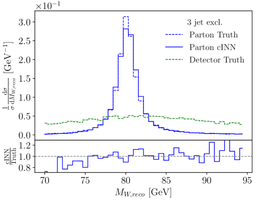
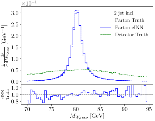
Figure 63: cINNed $p_{T,q}$ and $m_{W,\text{reco}}$ distributions. Training and testing events include exactly three (left) and four (right) jets from the data set including ISR. Figure from Ref. [43].

Next, we can demonstrate how the cINN unfolds a sample of events with a variable number of jets from the hard process and from ISR. First, we show the unfolding results for events with three jets in the upper panels of Fig. 63. For three jets in the final state, the combination of detector effects and ISR has a visible effect on the kinematics of the leading quark. This softening is correctly reversed by the unfolding. For the sub-leading quark the problem and the unfolding performance is similar to the exclusive 2-jet case. The situation becomes more interesting when we consider samples with two to four jets all combined. Now the network has to flexibly resolve the combinatorial problem to extract the two $W$-decay jets from a mixed training sample. In Fig. 63 we show a set of unfolded distributions from a variable jet number. Without showing them, it is clear that the $p_{T,j}$-threshold at the detector level is corrected, and the cINN allow for both $p_{T,q}$ values to zero. Next, we see that the comparably flat azimuthal angle difference at the parton level is reproduced to better than 10% over the entire range. Finally, the $m_{jj}$ distribution with a additional MMD loss re-generates the $W$-mass peak at the parton level almost perfectly. The precision of this unfolding is not any worse than it is for the INN generator in Sec. 4.3.3. This means that conditional generative networks unfold detector effects and jet radiation for LHC processes very well, even through their network architectures are more complex than the classifiers used in Sec. 5.1.

5.2.2 cINN inference

If a cINN can invert a forward simulation by generating a probability distribution in the target phase space from a Gaussian latent distribution, we should be able to use the same network to generate posterior probability distributions in model space. The network would also be conditioned on observed events, but the INN would link the Gaussian latent space to a multi-dimensional parameter space. We illustrate this inference task on the QCD splittings building up the parton shower. These splitting kernels are given in Eq.(3.4), and their common pre-factor has been measured with LEP data. In terms of the color factors these classic measurements give

$$C_{A}\equiv N_{c}=2.89\pm 0.21\qquad\text{and}\qquad C_{F}\equiv\frac{N_{c}^{2}-1}{2N_{c}}=1.30\pm 0.09\;.$$ (5.25)

For a more systematic approach to measuring the splitting kernels, organized in terms of the relative transverse momentum of the daughter particles in the splitting, we modify the strictly collinear splitting kernels of Eq.(3.4). We keep the argument $z$ describing the momentum fraction of the leading daughter parton, and parameterize the transverse momentum in the splitting using a new observable $y$, defined by

$$p_{T}^{2}=y\;z(1-z)\;.$$ (5.26)

In terms of the soft and collinear variables the relevant splitting kernels for massless QCD now read

$$P_{g\leftarrow g}(z,y) =C_{A}\bigg{[}D_{gg}\left(\frac{z(1-y)}{1-z(1-y)}+\frac{(1-z)(1-y)}{1-(1-z)(1-y)}\right)+F_{gg}z(1-z)+C_{gg}yz(1-z)\bigg{]}$$

$$P_{q\leftarrow q}(z,y) =C_{F}\left[D_{qq}\frac{2z(1-y)}{1-z(1-y)}+F_{qq}(1-z)+C_{qq}yz(1-z)\right]$$

$$P_{g\leftarrow q}(z,y) =\frac{1}{2}\left[F_{qq}\left(z^{2}+(1-z)^{2}\right)+C_{gq}yz(1-z)\right]\;.$$ (5.27)

The collinear expressions from Eq.(3.4) can be recovered in the limit $p_{T}^{2}\propto y\to 0$. We also include a set of free parameters to allow for possible deviations from the QCD results. To leading order in perturbative QCD they are

$$D_{qq,gg}=1\qquad\qquad F_{qq,gg}=1\qquad\qquad C_{qq,gg,gq}=0\;.$$ (5.28)

These parameters are a generalization of the $C_{A}$ vs $C_{F}$ measurements quoted in Eq.(5.25). The prefactors $D_{ij}$ would correspond to a universal correction like a two-loop anomalous dimension and resums sub-leading logarithms arising from the collinear splitting of soft gluons. Their measurements can largely be identified as

$$D_{qq}\sim C_{F}\qquad\text{and}\qquad D_{gg}\sim C_{A}\;.$$ (5.29)

The $F_{ij}$ modify the leading terms in $p_{T}$, truncated in the strong coupling. The rest terms $C_{ij}$ are defined through an additional factor $p_{T}^{2}$. The modified splitting kernels of Eq.(5.27) can be included in a Monte Carlo generator, for instance Sherpa.

Figure 64: BayesFlow setup of the cINN for training and inference. Figure from Ref.[44].

To extract the splitting parameters from measured jets $x$ we use the cINN architecture described in Sec. 5.2.1. The cINN-inference framework, also referred to as BayesFlow, is illustrated in Fig. 64. In the training phase we scan over model parameters $m$, in our case the modification factors with the QCD values given in Eq.(5.28), and generate the corresponding jets. The $m$-dependent simulated jet data is referred to as $x_{m}$. We then train a summary network combined with the cINN to map the model parameters $m$ onto a Gaussian latent space. This corresponds to the cINN unfolding in Fig. 61, with the parton-level events replaced by the model parameters and the conditional reconstruction-level events replaced by the simulated jets. The technical challenge in this application is that the training is fully amortized, which means we map the full set of training data onto the Gaussian latent space, which turns into a memory limitation to the amount of training data.

For the network evaluation or inference we sample from the Gaussian latent space into the model parameter space $m$ to generate a correlated posterior distribution of the allowed $D_{{}_{i}j}$, $F_{ij}$, and $C_{ij}$. If we want to interpret this framework in a Bayesian sense we can identify the starting distributions in model space, which we use to generate the training jets, as the prior, and the final inference outcome as the posterior.

Before applying BayesFlow to LHC jets including hadronization and detector simulation, we test the inference model on a simple toy shower. We simulate jets using the process

$$e^{+}e^{-}\to Z\to q\bar{q}\;,$$ (5.30)

with massless quarks and a hard showering cutoff at 1 GeV. Most jets appear close to the phase space boundary $p_{T,j}<m_{Z}/2$. For each event we apply the parton shower to one of the outgoing quarks, such that the second quark acts as the spectator for the the first splitting, and we only consider one jet. The network then analyses the set of outgoing momenta except for the initial spectator momentum. For the training data we scan the parameters $\{D_{ij},F_{ij},C_{ij}\}$ in two or three dimensions. The input to the summary network per batch are a sets of constituent 4-vectors, and we typically train on 100k randomly distributed points in model space. This number is much smaller than what we typically use for network training at the LHC.

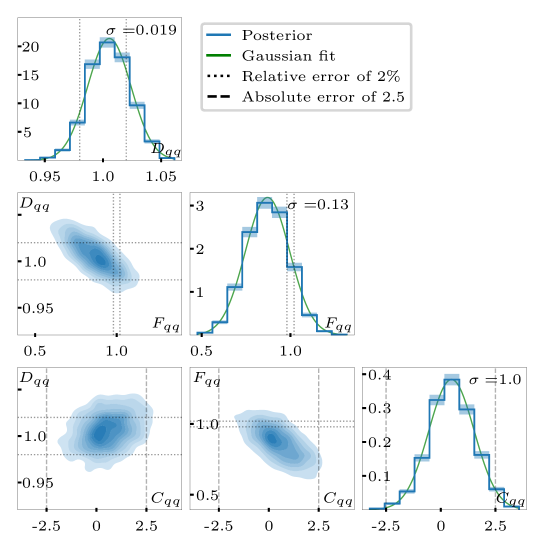
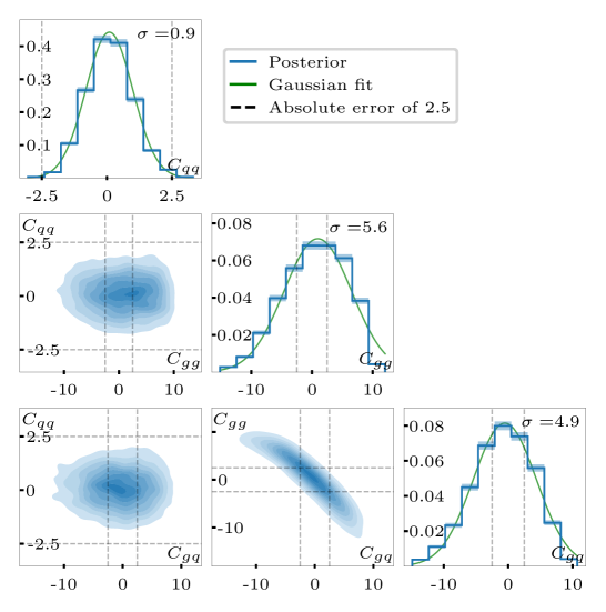
Figure 65: Posterior probabilities for the toy shower, gluon radiation only, $\{D_{qq},F_{qq},C_{qq}\}$ (left), and the $p_{T}$-suppressed rest terms for all QCD splittings, $\{C_{qq},C_{gg},C_{gq}\}$ (right). We assume SM-like jets. Figure from Ref. [44].

For our first test we restrict the shower to the $P_{qq}$ kernel, such that a hard quark successively radiates collinear and soft gluons. This way our 3-dimensional model space is given by

$$\{D_{qq},F_{qq},C_{qq}\}\;.$$ (5.31)

In the left panel of Fig. 65 we show the posterior probabilities for these model parameters assuming true SM-values. All 1-dimensional posteriors are approximately Gaussian. The best-measured parameter of the toy model is the regularized divergence, followed by the finite terms, and then the rest term with its assumed $p_{T}$-suppression. This reflects the hierarchical structure of the splitting kernel. The correlations between parameters are small, but not negligible.

In a second step we include all QCD splitting kernels from Eq.(5.27) and target the unknown rest terms

$$\{C_{qq},C_{qg},C_{gg}\}\;.$$ (5.32)

This means we assume our perturbative predictions for the leading contributions to hold, so we need to estimate the uncertainty of the perturbative description. For $C_{qq}$ the error bar shrinks slightly, in the absence of the dominant contributions to this kernel. For the other two rest terms, $C_{gg}$ and $C_{gq}$, we find significantly larger error bars and a strong anti-correlation.

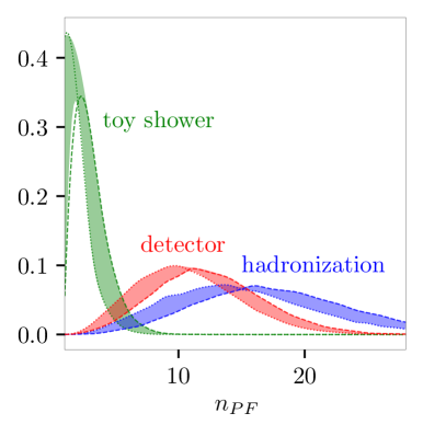
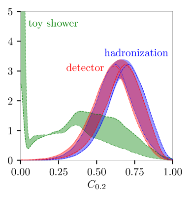
Figure 66: High-level observables $n_{\text{PF}}$ and $C_{0.2}$ for 100k jets. We show the distributions for the toy shower, the Sherpa shower with hadronization, and including a detector simulation The bands indicate the variation of $D_{qq}=0.5.~{}...~{}2$ (dotted and dashed). Figure from Ref. [44].

For a more realistic simulation we rely on a full Sherpa shower with hadronization and a fast detector simulation. The dataset consists of our usual particle flow objects forming the jet. Unlike for the classification of boosted jets we study relatively soft jets, again simulated from $Z$-decays with a spectrum

$$p_{T,j}=20~{}\text{GeV}~{}...~{}\frac{m_{Z}}{2}\;.$$ (5.33)

To illustrate the physics limiting the measurement, we show two high-level observables from Eq.(1.6) for the toy shower, after hadronization, and after detector effects in Fig. 66. The shaded bands reflect a variation $D_{qq}=0.5.~{}...~{}2$. The number of constituents $n_{\text{PF}}$ generally increases with $D_{qq}$. The toy shower with a high cutoff and no hadronization does not generate a very large number of particle flow objects. Hadronization increases the number of constituents significantly, but is not related to QCD splittings. The finite detector resolution and the detector thresholds decreases $n_{\text{PF}}$ again. The constituent-constituent correlation $C_{0.2}$ loses all toy events at small values when we include hadronization, while the broad feature around $C_{0.2}\sim 0.4$ narrows and moves to slightly larger values. The main message from Fig. 66 is that from a QCD point of view the hadronization effects are qualitatively and quantitatively far more important than the detector effects.

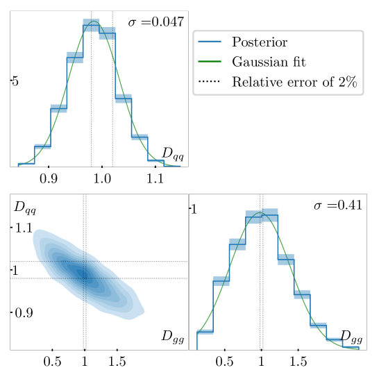
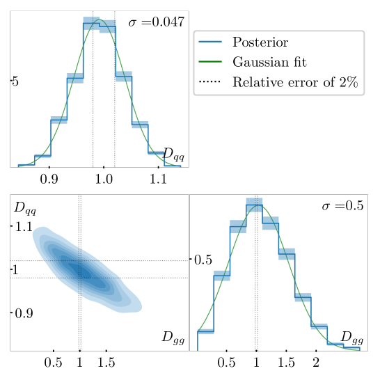
Figure 67: Posterior probabilities for the Sherpa shower, soft-collinear leading terms for all QCD splittings, $\{D_{qq},D_{gg}\}$. We assume SM-like jets and show results without Delphes detector simulation (left) and including detector effects (right). Figure from Ref. [44].

To simplify the task in view of the hadronization effects we allow for all QCD splittings, but only measure the leading soft-collinear contributions, corresponding to $C_{F}$ and $C_{A}$,

$$\{D_{qq},D_{gg}\}\;.$$ (5.34)

The results are shown in Fig. 67. First, we see that the measurement after hadronization only and after hadronization and detector effects is not very different. In both cases we see a significant degradation of the measurements, especially in $D_{gg}$, and a strong correlation which reflects the fact that we are only looking at quark-induced jets. For an actual measurement this correlation could be easily removed by combining quark-dominated and gluon-dominated samples.

5.3 Simulation-based inference

As simulation-based inference we consider a wide range of methods which all share the basic idea that we want to use likelihoods to extract information from data, ideally event by event, but the likelihood is not accessible explicitly. Likelihoods have been a theme for all our ML-applications, starting with the network training introduced in Sec. (1.2.1). In this section we will be a little more specific and introduce two ways we can use modern ML-methods to infer fundamental (model) parameters from LHC data.

5.3.1 Likelihood extraction

In spite of discussing likelihoods and likelihood ratios several times, we have never written down the likelihood as we use it in an analysis of datasets consisting of unweighted and uncorrelated events. A likelihood for a counting experiment can be split into the statistical probability of observing $n$ event with $b$ background events expected, and a normalized probability of observing individual events in a given phase space point. If we phrase the question in terms of a hypothesis or set of model parameters $\theta_{B}$ we can write

$$\boxed{p(x|\theta_{B})=\text{Pois}(n|b)\;\prod_{i=1}^{n}f_{B}(x_{i})}\qquad\text{with}\qquad\text{Pois}(n|b)=\frac{b^{n}}{n!}\;e^{-b}\;.$$ (5.35)

The Neyman–Pearson lemma then tells us that if we want to, for instance, decide between a background-only and signal-plus-background hypothesis we will find optimal results by using the likelihood ratio as the estimator

$$\frac{p(x|\theta_{S+B})}{p(x|\theta_{B})} =\frac{\text{Pois}(n|s+b)\;\prod_{i}f_{S+B}(x_{i})}{\text{Pois}(n|b)\;\prod_{i}f_{B}(x_{i})}$$

$$=e^{-s}\left(\frac{s+b}{b}\right)^{n}\;\frac{\prod_{i}f_{S+B}(x_{i})}{\prod_{i}f_{B}(x_{i})}$$

$$=e^{-s}\;\frac{\prod_{i}(s+b)f_{S+B}(x_{i})}{\prod_{i}bf_{B}(x_{i})}\ =e^{-s}\;\frac{\prod_{i}[sf_{S}(x_{i})+bf_{B}(x_{i})}{\prod_{i}bf_{B}(x_{i})]}\;.$$ (5.36)

We have used the assumption that $s+b$ signal plus background events follow weighted signal and background distributions independently. We can translate this into the log-likelihood ratio as a function of the transition amplitudes $f(x)$ over phase space, noticing that the log-likelihood ratio is additive for phase space points or events $x_{i}$,

$$\log\frac{p(x|\theta_{S+B})}{p(x|\theta_{B})}=-s+\sum_{i}\log\left[1+\frac{sf_{S}(x_{i})}{bf_{B}(x_{i})}\right]\;.$$ (5.37)

If we work with simulation only, consider irreducible backgrounds at the parton level, and limit ourselves to the same partons in the initial state, we can compute the log-likelihood ratio as

$$\log\frac{p(x|\theta_{S+B})}{p(x|\theta_{B})}=-s+\sum_{i}\log\left[1+\frac{|\mathcal{M}_{S}(x_{i})|^{2}}{|\mathcal{M}_{B}(x_{i})|^{2}}\right]\;.$$ (5.38)

Prefactors relating the transition matrix element to the fully exclusive cross sections, including parton densities, will drop out of the ratio of signal and backgrounds. This means we can use Eq.(5.37) to compute the maximum possible significance for observing a signal over a background integrating over matched signal and background event samples. Moving from two equal hypotheses, signal vs background, to measuring a parameter $\theta$ around a reference value $\theta_{\text{ref}}$ we can rewrite the corresponding likelihood ratio

$$\log\frac{p(x|\theta)}{p_{\text{ref}}(x)}=-s+\sum_{i}\log\left[1+\frac{|\mathcal{M}(x_{i}|\theta)|^{2}}{|\mathcal{M}(x_{i})|_{\text{ref}}^{2}}\right]\qquad\text{with}\qquad p_{\text{ref}}(x)\equiv p(x|\theta_{\text{ref}})\;.$$ (5.39)

If we are interested in parameter values $\theta$ close to a reference point $\theta_{\text{ref}}$, we can simplify our problem and taylor the log likelihood around $\theta_{\text{ref}}$,

$$\log\frac{p(x|\theta)}{p(x|\theta_{\text{ref}})}=(\theta-\theta_{\text{ref}})\underbrace{\frac{\partial}{\partial\theta}\log p(x|\theta)\Bigg{|}_{\theta_{\text{ref}}}}_{t(x|\theta_{\text{ref}})}+\mathcal{O}\left((\theta-\theta_{\text{ref}})^{2}\right)\;.$$ (5.40)

The leading term is called the score in statistics or optimal observable in particle physics. Neglecting the higher-order terms we solve this equation and find

$$p(x|\theta)\approx e^{t(x|\theta_{\text{ref}})(\theta-\theta_{\text{ref}})}\;p(x|\theta_{\text{ref}})\,.$$ (5.41)

This relation to the likelihood function implies that the score $t(x|\theta_{\text{ref}})$ are its sufficient statistics. If we measure it we capture all information on $\theta$ included in the the full event record $x$. It is possible to show that the score is not only linked to the Neyman-Pearson lemma for discrete hypotheses $H_{S+B}$ vs $H_{B}$, but also saturates the Cramér-Rao bound for a continuous parameter measurement $\theta\sim\theta_{\text{ref}}$.

For the application of modern ML-methods to likelihood extraction we follow the approach of the public analysis tool MadMiner [45, 46]. In Sec. 3.1 we have already seen how we can use the likelihood ratio for event classification. The starting point is the likelihood ratio trick, where we assume that an ideal discriminator $D$ has to reproduce the likelihood ratio. To see this we start from the optimally trained discriminator in Eq.(4.19), translate the output into our new conventions, and solve for the likelihood ratio,

$$D_{\text{opt}}(x) =\frac{p_{\text{ref}}(x)}{p_{\text{ref}}(x)+p(x|\theta)}=\frac{1}{1+\dfrac{p(x|\theta)}{p_{\text{ref}}(x)}}$$

$$\Leftrightarrow\qquad\frac{p(x|\theta)}{p_{\text{ref}}(x)} =\frac{1-D_{\text{opt}}(x)}{D_{\text{opt}}(x)}\;.$$ (5.42)

To construct this estimator for the likelihood ratio we start by generating two training datasets, one following $p_{\text{ref}}(x)$ and one following $p(x|\theta)$. In a slight variation of the two-hypothesis classification we now train a $\theta$-dependent classifier, where $\theta$ enters the training as a condition. After training, we can use the output of this classifier for a given value of $\theta$ as a numerical approximation to the likelihood ratio $p(x|\theta)/p_{\text{ref}}(x)$. This approach has the advantage that we only need to train a stable classification network. The advantage of this method is that it is fast for a limited number of phase space points, as long as the network has converged on a smooth classification output. In the MadMiner implementation this approach is called calibrated ratios of likelihoods (Carl).

For a second approach, we go beyond classification and train a regression network to encode likelihoods or likelihood ratios over the combined phase space and parameter space $(x,\theta)$. For this purpose we modify the relation between the likelihood ratio given in Eq.(5.39) and the matrix elements using an approximate factorization for LHC physics including a range of latent variables. We start with the observation that we can write the likelihood in $x$ as an integral over latent variables which describe the hard process $z_{p}$, the step to the parton shower $z_{s}$, and to the detector level $z_{d}$. We can also assume that our parameter of interest only affects the hard scatting,

$$p(x|\theta)=\int dz\;p(x,z|\theta)\approx\int dz_{d}dz_{s}dz_{p}\;p(x|z_{d})\;p(z_{d}|z_{s})\;p(z_{s}|z_{p})\;p(z_{p}|\theta)\;.$$ (5.43)

Using this factorization we see that the problem with the likelihood ratio is that it is given by a ratio of two integrals, for which there is no easy and efficient way to evaluate it, even using modern ML-methods,

$$\frac{p(x|\theta)}{p_{\text{ref}}(x)}=\frac{\int dz\;p(x,z|\theta)}{\int dz\;p_{\text{ref}}(x,z)}\;.$$ (5.44)

However, we can simplify the problem using the property of the joint likelihood ratio being an unbiased estimator of the likelihood ratio. This means we can evaluate the ratio of the joint likelihoods instead of the ratio of the likelihoods,

$$\frac{p(x,z|\theta)}{p_{\text{ref}}(x,z)}\approx\frac{p(z_{p}|\theta)}{p_{\text{ref}}(z_{p})}=\frac{|\mathcal{M}(z_{p}|\theta)|^{2}}{|\mathcal{M}_{\text{ref}}(z_{p})|^{2}}\;\frac{\sigma_{\text{ref}}}{\sigma(\theta)}\;.$$ (5.45)

In the last step we do not assume that all prefactors in the relation between matrix element and rate cancel, so we ensure the correct normalization explicitly. The advantage of using the joint likelihood ratio as an estimator for the likelihood ratio is that we can encode it in a network comparably easily, using the factorization properties of LHC rates.

Inspired by the fact that the joint likelihood ratio can serve as an estimator for the actual likelihood ratio we can try to numerically extract the likelihood ratio from the joint likelihood ratio. If we assume that we have a dataset encoding the likelihood ratio over phase space we still need to encode it in a network. We simplify our notation from Eq.(5.43) to

$$p(x,z|\theta)=p(x|z_{p})\;p(z_{p}|\theta)\qquad\text{or}\qquad p(x|\theta) =\int dz_{p}\;p(x,z_{p}|\theta)$$

$$\approx\int dz_{p}\;p(x|z_{p})\;p(z_{p}|\theta)\;.$$ (5.46)

Slightly generalizing the problem we can ask if it is possible to construct proxies for $(x,z_{p})$-dependent distributions as $x$-dependent distributions, with a given test function. This is similar to the variational approximation introduced in Sec. 1.2.4. We will see that the test function $p(x|z_{p})p(z_{p}|\theta)$ combined with an L2 norm over the two functions will turn out useful

$$F(x)=\int dz_{p}\;\left[f(x,z_{p})-\hat{f}(x)\right]^{2}\;p(x|z_{p})\;p_{\text{ref}}(z_{p})\;.$$ (5.47)

The variational condition defines the approximation $\hat{f}_{*}(x)$ through a minimization of $F(x)$,

$$0=\frac{\delta F}{\delta\hat{f}} =\frac{\delta}{\delta\hat{f}}\int dz_{p}\;\left[f(x,z_{p})-\hat{f}(x)\right]^{2}\;p(x|z_{p})\;p_{\text{ref}}(z_{p})$$

$$=\int dz_{p}\;p(x|z_{p})\;p_{\text{ref}}(z_{p})\;\frac{\delta}{\delta\hat{f}}\left[f(x,z_{p})-\hat{f}(x)\right]^{2}$$

$$=-2\int dz_{p}\;p(x|z_{p})\;p_{\text{ref}}(z_{p})\;\left[f(x,z_{p})-\hat{f}(x)\right]$$

$$\Leftrightarrow\qquad\hat{f}_{*}(x) =\frac{\int dz_{p}\;f(x,z_{p})\;p(x|z_{p})\;p_{\text{ref}}(z_{p})}{\int dz_{p}\;p(x|z_{p})\;p_{\text{ref}}(z_{p})}=\frac{\int dz_{p}\;f(x,z_{p})\;p(x|z_{p})\;p_{\text{ref}}(z_{p})}{p_{\text{ref}}(x)}\;.$$ (5.48)

We can apply this method to the joint likelihood ratio from Eq.(5.45) and find

$$f(x,z_{p}) =\frac{p(z_{p}|\theta)}{p_{\text{ref}}(z_{p})}\approx\frac{p(x|z_{p})\;p(z_{p}|\theta)}{p(x|z_{p})\;p_{\text{ref}}(z_{p})}$$

$$\Rightarrow\qquad\hat{f}_{*}(x) =\frac{\int dz_{p}\;f(x,z_{p})\;p(x|z_{p})\;p(z_{p}|\theta)}{p_{\text{ref}}(x)}=\frac{p(x|\theta)}{p_{\text{ref}}(x)}\;.$$ (5.49)

This means that by numerically minimising Eq.(5.47) as a loss function we can train a regression network for reproduce the likelihood ratio from Eq.(5.39).

The third, and final approach to extract likelihoods for the LHC starts with remembering that according to Eq.(5.40) the derivative of the log-likelihood ratio is a sufficient statistics for a parameter of interest $\theta$ in the region around $\theta_{\text{ref}}$. This leads us to computing the joint score

$$t(x,z|\theta) =\frac{\partial}{\partial\theta}\log p(x,z|\theta)=\frac{1}{p(x,z|\theta)}\;\frac{\partial}{\partial\theta}p(x,z|\theta)$$

$$\approx\frac{p(x|z_{d})\;p(z_{d}|z_{s})\;p(z_{s}|z_{p})}{p(x|z_{d})\;p(z_{d}|z_{s})\;p(z_{s}|z_{p})\;p(z_{p}|\theta)}\;\frac{\partial}{\partial\theta}p(z_{p}|\theta)=\frac{\partial p(z_{p}|\theta)/\partial\theta}{\partial(z_{p}|\theta)}$$

$$=\frac{\sigma(\theta)}{|\mathcal{M}(z_{p}|\theta)|^{2}}\;\frac{\partial}{\partial\theta}\frac{|\mathcal{M}(z_{p}|\theta)|^{2}}{\sigma(\theta)}=\frac{\partial|\mathcal{M}(z_{p}|\theta)|^{2}/\partial\theta}{|\mathcal{M}(z_{p}|\theta)|^{2}}-\frac{\partial\sigma(\theta)/\partial\theta}{\sigma(\theta)}\;,$$ (5.50)

and limit our analysis to $\theta\sim\theta_{\text{ref}}$. Just as for the joint likelihood ratio we use the variational approximation from Eq.(5.48) to train a network for the score. This time we define, in the simplified notation of Eq.(5.46),

$$F(x) =\int dz_{p}\;\left[f(x,z_{p})-\hat{f}(x)\right]^{2}\;p(x|z_{p})\;p(z_{p}|\theta)$$

$$f(x,z_{p}) =t(x,z_{p}|\theta)=\frac{p(x|z_{p})\;\partial p(z_{p}|\theta)/\partial\theta}{p(x|z_{p})\;p(z_{p}|\theta)}$$

$$\Rightarrow\qquad\hat{f}_{*}(x) =\frac{\int dz_{p}\;f(x,z_{p})\;p(x|z_{p})\;p(z_{p}|\theta)}{\int dz_{p}\;p(x|z_{p})\;p(z_{p}|\theta)}=\frac{\int dz_{p}\;p(x|z_{p})\;\partial p(z_{p}|\theta)/\partial\theta}{p(x|\theta)}=t(x|\theta)\;.$$ (5.51)

This means we can also encode the score as the local summary statistics for a model parameter $\theta$ in a network using a variational approximation. In MadMiner this method is called score approximates likelihood locally or Sally.

To illustrate this score extraction we look at the way heavy new physics affects the Higgs production channel

$$pp\to WH\to\ell\bar{\nu}\;b\bar{b}\;.$$ (5.52)

If we assume that new particles are heavy and not produced on-shell, the appropriate QFT description is higher-dimensional operators and the corresponding Wilson coefficients. The effective Lagrangian we use to describe LHC observation then becomes

$$\mathscr{L}=\mathscr{L}_{\text{SM}}+\sum_{d,k}\frac{C_{k}^{d}}{\Lambda^{d-4}}\mathcal{O}_{k}^{d}\;.$$ (5.53)

We can organize the effective Lagrangian by the power $d$ of the scale of the unknown new physics effects, $\Lambda$. The coupling parameters $C_{k}$ are called Wilson coefficients. The Lagrangian of the renormalizable Standard Model has mass dimension four, there exists exactly one operators at dimension five, related to the neutrino mass, and 59 independent operators linking the Standard Model particles at dimension six. Adding flavor indices increases this number very significantly. The $WH$ production process mostly tests three of them,

$$\mathcal{O}_{HD} =(\phi^{\dagger}\phi)\square(\phi^{\dagger}\phi)-\frac{1}{4}(\phi^{\dagger}D^{\mu}\phi)^{*}(\phi^{\dagger}D_{\mu}\phi)$$

$$\mathcal{O}_{HW} =\phi^{\dagger}\phi W_{\mu\nu}^{a}W^{\mu\nu a}$$

$$\mathcal{O}_{Hq}^{(3)} =(\mbox{${\phi^{\dagger}i\,\raisebox{5.69054pt}{\boldmath${}^{\leftrightarrow}$}D_{\mu}^{\,a}\,\phi}$})({\overline{Q}}_{L}\sigma^{a}\gamma^{\mu}Q_{L})\;,$$ (5.54)

where $\phi$ is the Higgs doublet, $D_{\mu}$ the full covariant derivative, $W_{\mu\nu}^{a}$ the weak field strength, and $\mbox{${\phi^{\dagger}i\,\raisebox{5.69054pt}{\boldmath${}^{\leftrightarrow}$}D_{\mu}^{\,a}\,\phi}$}=i\phi^{\dagger}(\frac{\sigma^{a}}{2}D_{\mu}\phi)-i(D_{\mu}\phi)^{\dagger}\frac{\sigma^{a}}{2}\phi$. The three operators affect the transition amplitude for $WH$ production in different ways. In principle, dimension-6 operators can come with up to two derivatives, which after a Fourier transformation turn into two powers of the momentum transfer in the interaction, $p^{2}/\Lambda^{2}$. Of the three operators in Eq.(5.54) it turns out that $\mathcal{O}_{HD}$ induces a finite and universal contribution to the Higgs wave function, turning into a rescaling to all single-Higgs interactions. In contrast, $\mathcal{O}_{HW}$ changes the momentum structure of the $WWH$ vertex and leads to momentum-enhanced effects in the $WH$ final state. The operator $C_{Hq}^{(3)}$ has the unusual feature that it induces a $q{\overline{q}}^{\prime}WH$ 4-point interaction which avoids the $s$-channel suppression of the SM-process and also leads to a momentum enhancement in the $WH$ kinematics.

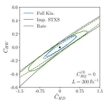
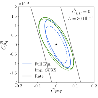
Figure 68: Expected exclusion limits from rates only (grey), simplified template cross sections (green), and using Sally to extract the score. Limits based on a linearized description in the Wilson coefficients are shown as dashed lines, while the solid lines also include squared contributions of the operators defined in Eq.(5.54). Figure from Ref. [47].

Based on what we know about the effects of the operators, we can study their effects in the total production rate and a few specific kinematic distributions,

$$\sigma_{WH}\qquad\qquad p_{T,W}\approx p_{T,H}\qquad\qquad m_{T,\text{tot}}\sim m_{WH}\;.$$ (5.55)

Because of the neutrino in the final state it is hard to reconstruct the invariant mass of the $WH$ final state, so we can use a transverse mass construction as the usual proxy. These transverse mass constructions typically replace the neutrino 3-momentum with the measured missing transverse momentum and have a sharp upper cutoff at the invariant mass, more details are given in Ref. [3].

For the simple $2\to 2$ signal process given in Eq.(5.52) we would expect that the number of independent kinematic variables is limited. At the parton level a $2\to 2$ scattering process can be described by the scattering angle, the azimuthal angle represents a symmetry, and the embedding of the partonic process into the hadronic process can be described by the energy of the partonic scattering as a second variable. This means, measuring Wilson coefficients from 2-dimensional kinematic correlations should be sufficient. This leads to a definition of a set of improved simplified template cross sections (STXS) in terms of the two kinematic variables given in Eq.(5.55). The extraction of the score using the Sally method allows us to benchmark this 2-dimensional approach and to quantify how much of the entire available information is captured by them.

In Fig. 68 we show two slices in the model space spanned by the operators and Wilson coefficients given in Eq.(5.54). In the left panel we first see that even for two operators the rate measurement leaves us with an approximately flat direction in model space. Adding 2-dimensional kinematic information breaks this flat directions, but this breaking really requires us to also include the squared contributions of the Wilson coefficients, specifically $\mathcal{O}_{HW}$. Using the full phase space information leads to significantly better results, even for the simple $2\to 2$ process. The reason is that we are not really comparing the SM-predictions and the dimension-6 signal hypothesis, but are also including the continuum background to $\ell\bar{\nu}b\bar{b}$ production, and in the tails of the signal kinematics this continuum background becomes our leading limitation. In the right panel of Fig. 68 we show another slice through the model parameter space, now omitting the operator $\mathcal{O}_{HD}$ which is only constrained by the total $WH$ rate. Again, we have a perfectly flat direction from the rate measurement, but the two remaining operators can be distinguished already in the linearized description from their effects over phase space, and the 2-dimensional kinematic information captures most of the effects encoded in the full likelihoods. This example is not an actual measurement, but only a study for the LHC Run 3, but it shows how we can employ simulation-based inference in a more classical way, with binned kinematic distributions, and using the full likelihood information. It should be obvious which methods does better.

5.3.2 Flow-based anomaly detection

Now that we can extract likelihoods from event samples, we need to ask what kind of data we would train on. In the last section we used supervised training on simulated event samples for this purpose. An alternative way would be to use measured data to extract likelihoods. Obviously, this has to be done with some level of unsupervised training. In Sec. 3.1 we introduced the CWoLa method and its application to bump hunt searches for BSM physics. Our goal is to use unsupervised likelihood extraction to enhance such bump hunts.

The general setup of such searches is illustrated in Fig. 69: We start with a smooth feature $m$, for example the di-jet or di-lepton invariant mass, and look for signal bumps rising above the falling background. In addition, we assume that the signal corresponds a local overdensity in other event features, collectively referred to as $x$. The problem we want to address is how to estimate for the background in a data-driven way all over phase space. Usually, one defines a signal region (SR) and a side band (SB), and estimates the amount of background in the signal region based on the side bands. One then scans over different signal region hypotheses, covering the full feature space in $m$. A simple technical method is to fit the $m$-distribution, remove individual bins, and look for a change in $\chi^{2}$. This data-driven approach has the advantage that it does not suffer from imperfect background simulations. In the Higgs discovery plots it looks like this is what ATLAS and CMS did, but this is not quite true, because the information on the additional features in $x$ was crucial to enhance the statistical power of the side band analysis. Using the machine-learning techniques we discussed so far, we can approach this problem from several angles.

As always, the Neyman-Pearson lemma ensures that the best discriminator between two hypotheses is the likelihood ratio, with the specific relation given in Eqs.(4.19) and (5.42). The key point of the CWoLa method in Sec. 3.1 is that a network classifier learns a monotonic function of this ratio, if the two training dataset have different compositions of signal and background. If we identify the two training datasets with a data-driven modelling of the background likelihood and a measured signal+background likelihood we can use CWoLa to train a signal vs background classifier using the link

$$\frac{x\sim p_{\text{data}}(x|m\in SR)}{x\sim p_{\text{data}}(x|m\in SB)}\;\stackrel{{\scriptstyle\text{class}}}{{\longrightarrow}}\frac{p_{S+B}(x)}{p_{B}(x)}\;\to\;\frac{p_{S}(x)}{p_{B}(x)}\;.$$ (5.56)

In the last CWoLa step we train a classifier to distinguish events from the signal and background regions, only using the features $x$ and not $m$. The challenge with this method is the fine print in the CWoLa method, which essentially requires $m$ and $x$ to not be correlated, so we can ignore the fact that in Eq.(5.56) the numerator and denominator are evaluated in different phase space regions.

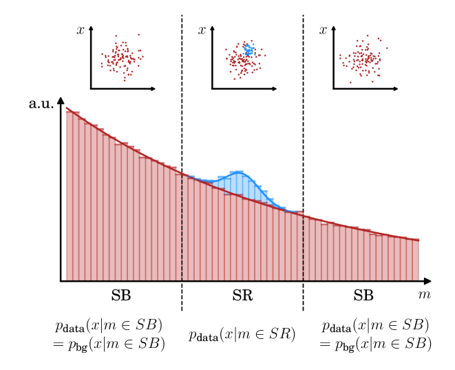
Figure 69: Definition of signal region (SR) and side band (SB). The red distribution is the assumed background, the blue is the signal. Features of the events other than $m$ are called $x$. Figure from from Ref.[48].

If we could use some kind of network to access likelihoods directly, this would allow us to construct the likelihood ratio simply as a ratio of two independently learned likelihoods. This method is called ANOmaly detection with Density Estimation or Anode. Here, one flow learns the assumed background density from the side bands, $p_{\text{model}}(x|m\in SB)$, where the label ‘model’ indicates that we will use this distribution to model the background in the signal region. Since the label $m$ is a continuous variable, we can extract the density of events in the signal region from $p_{\text{model}}(x|m)$ simply by passing events with $m\in SR$ through it and using the network to interpolate in $m$. For this to happen, the flows have to learn the conditional density $p(x|m)$ instead of the joint density $p(x,m)$ because we need to be able to interpolate into the signal region to compute $p_{\text{model}}(x|m\in SR)$. A flow that learns $p(x,m)$ and then sees $m\notin SR$ will naturally return $p(x,m\in SR)=0$ instead of interpolating from the side bands into the signal region. This means Anode approximates the data distribution in the background regions and then relies on an interpolation to reach the signal region,

$$p_{\text{data}}(x|m\in SB)\;\stackrel{{\scriptstyle\text{train}}}{{\longrightarrow}}p_{\text{model}}(x|m\in SB)\;\stackrel{{\scriptstyle\text{interpolate}}}{{\longrightarrow}}p_{\text{model}}(x|m\in SR)\;.$$ (5.57)

The interpolated $p_{\text{model}}(x|m)$ for all $m$ is given by the red distribution in Fig. 69. The second network directly learns a hypothetical signal-plus-background density from the signal region $p_{\text{data}}(x|m\in SR)$. The learned density in the signal region includes the hypothetical signal, trained in an unsupervised manner. We can now form the ratio of the two learned densities in the signal region, each encoded in a network,

$$\frac{p_{\text{data}}(x|m\in SR)}{p_{\text{model}}(x|m\in SR)}\;,$$ (5.58)

which approaches the desired log-likelihood ratio and can be used for analysis.

Finally, we can go beyond classification and density estimation and make use of the fact that normalizing flows are not only density estimators, but generative models. The corresponding method of enhancing a bump hunt is to combine the ideas of CWoLa and Anode to Classifying Anomalies THrough Outer Density Estimation or Cathode. First, we learn the distribution of events in the side band, $p_{\text{model}}(x|m\in SB)$, just like in the Anode approach. Second, using this density estimator, $p_{\text{model}}(x|m)$, we sample artificial events in the signal region

$$p_{\text{data}}(x|m\in SB)\;\stackrel{{\scriptstyle\text{train}}}{{\longrightarrow}}p_{\text{model}}(x|m\in SB)\;\stackrel{{\scriptstyle\text{sample}}}{{\longrightarrow}}x\sim p_{\text{model}}(x|m\in SR)\;.$$ (5.59)

To guarantee the correct distribution of the continuous condition $m$ we use a kernel density estimator. This is a parameter-free method for density estimation, where for instance a Gaussian kernel is placed at each element of the dataset and the sum of all Gaussians at a given point is an estimator for the points density. Selecting a Gaussian at random and sampling from it draws samples from this distribution. The method is less efficient than normalizing flows, especially at high dimensions and for large datasets, but it is well-suited to model the $m$-dependence in the signal region from the side bands.

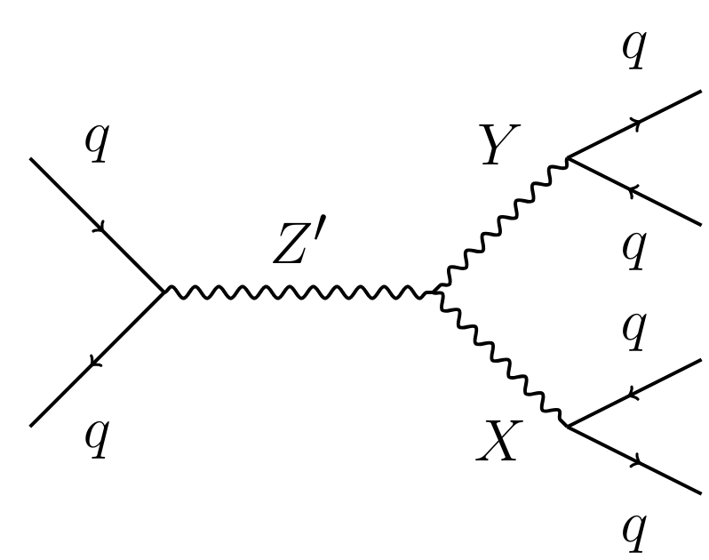
Figure 70: Signal process in the LHC Olympics R&D dataset, from Ref. [49].

The sampled events will follow the distribution $p_{\text{model}}(x|m\in SR)$, expected for background-only events in the signal region and again corresponding to the red distribution in Fig. 69. If there are actual signal events in the signal region we can use the two datasets following $p_{\text{model}}(x|m\in SR)$ and $p_{\text{data}}(x|m\in SR)$ to train a CWoLa classifier, as illustrated in Eq.(5.56). This means the third step of Cathode is to apply the CWoLa method: we train a classifier to distinguish the generated events from the data in the signal region. If there is a signal present, the classifier learns to distinguish the two sets based on the log-likelihood ratio argument of Eq.(3.2).

Cathode has several advantages over the other bump-hunt enhancing algorithms. First, unlike for CWoLa the data and the generated samples have $m\in SR$, so even when the features $x$ are correlated with $m$, the classifier will not learn to distinguish the sets by deducing the value of $m$ from $x$. Second, in contrast to CWoLa, the amount of training data is not limited. Cathode can oversample events in the signal region. which improves the quality of the classifier the same way we have seen with GANplification in Sec. 4.2.3 and super-resolution in Sec. 4.2.6. Finally, compared to Anode, the likelihood-ratio in Eq.(5.58) is learned from a classifier and not constructed as a ratio of two learned log-likelihoods. This is easier and gives more stable results.

As an application we compare CWola, Anode, and Cathode to a standard new-physics searches dataset, namely the LHC Olympics R&D dataset. This dataset consists of simulated di-jet events from Pythia and with the fast detector simulation Delphes. It includes 1M QCD di-jet events as background and 1k signal events describing the process

$$Z^{\prime}\to X(\to qq)Y(\to qq)\qquad\text{with}\quad m_{Z^{\prime}}=3.5~{}\text{TeV},m_{X}=500~{}\text{GeV},m_{Y}=100~{}\text{GeV}\;.$$ (5.60)

All events are required to satisfy a single-jet trigger with $p_{T}>1.2$ TeV. We use the kinematic training features

$$\{\;m_{j_{1}j_{2}},m_{j_{1}},m_{j_{2}}-m_{j_{1}},\tau_{21}^{j_{1}},\tau_{21}^{j_{2}}\;\}\;.$$ (5.61)

Here $j_{1}$ and $j_{2}$ refer to the two highest-$p_{T}$ jets ordered by jet mass ($m_{j_{1}}<m_{j_{2}}$), and $\tau_{ij}\equiv\tau_{i}/\tau_{j}$ are their $n$-subjettiness ratios defined in Eq.(2.13). The di-jet invariant mass $m_{j_{1}j_{2}}$ defines the signal and side band regions through

$$SR:\quad m_{jj}=3.3~{}...~{}3.7~{}\text{TeV}\;.$$ (5.62)

In Fig. 71 we see how the three methods perform in terms of the significance improvement characteristic (SIC), which gives the improvement factor of the statistical significance $S/\sqrt{B}$. The supervised anomaly detector as a reference is given by a classifier trained to distinguish perfectly modeled signal from background. The idealized anomaly detector shows the best possible performance of a data-driven anomaly detector. It is trained to distinguish perfectly modeled background from the signal plus background events in the signal region. Of the three methods Cathode clearly outperforms Anode and CWoLa and approaches the idealized anomaly detection over a wide range of signal efficiencies, indicating that the distribution of artificial events in the signal region follows the true background distribution closely.

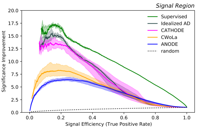
Figure 71: Significance improvement characteristic (SIC) for different bump-hunting methods. Figure from Ref. [48].

5.3.3 Symbolic regression of optimal observables

After learning how to extract likelihood ratios for a given inference task from simulations and from data, we want to return to particle theory and ask what we can learn from these numerical methods for particle theory. This is an example where we expect a numerical code or a neural network to correspond, at least approximately, to a formula. At least for physics, such an approximate formula would be the perfect explanation or illustration of our neural network. Formulas also have practical advantages over neural networks — we know that neural networks are great at interpolating, but usually provide very poor extrapolations. If we combine networks with formulas as models, these formulas will provide a much better extrapolation. This means is that in a field where all improvements in precision involve a step from analytic to numerical expressions, we need a way to at least approximately invert this direction. This is a little different from typical applications of symbolid regression, where we start from some kind of data, use a neural network to extract the relevant information, and then turn this relevant information into a formula. We really just want to see a formula for a neural network in the sense of explainable AI.

In Eq.(5.40) we have introduced the score or the optimal observable for the model parameter $\theta$ in a completely abstract manner, and in Sec. 5.3.2 we have deliberately avoided all ways to understand the likelihood ratio in terms of theory or simulations. However, in many LHC applications, for example in measuring the SMEFT Wilson coefficients defined in Eq.(5.54), we can at least approximately extract the score or optimal observables. For those Wilson coefficients the natural reference point is the Standard Model, $\theta_{\text{ref}}=0$. At parton level and assuming all particle properties can be observed, we know from Eq.(5.39) that the likelihood is proportional to the transition amplitude,

$$p(x|\theta)\propto|\mathcal{M}(x|\theta)|^{2}=|\mathcal{M}(x)|^{2}_{\text{ref}}+\theta|\mathcal{M}(x)|^{2}_{\text{int}}+\mathcal{O}(\theta^{2})\;,$$ (5.63)

where $|\mathcal{M}|^{2}_{\text{int}}$ denotes the contribution of the interference term between Standard Model and new physics to the complete matrix element. In that case the score becomes

$$t(x|\theta_{\text{ref}}=0)=\frac{|\mathcal{M}(x)|^{2}_{\text{int}}}{|\mathcal{M}(x)|^{2}_{\text{ref}}}\;.$$ (5.64)

This formula illustrates that the score does not necessarily have to be an abstract numerical expression, but that we should be able to encode it in a simple formula, at least in a perturbative approach.

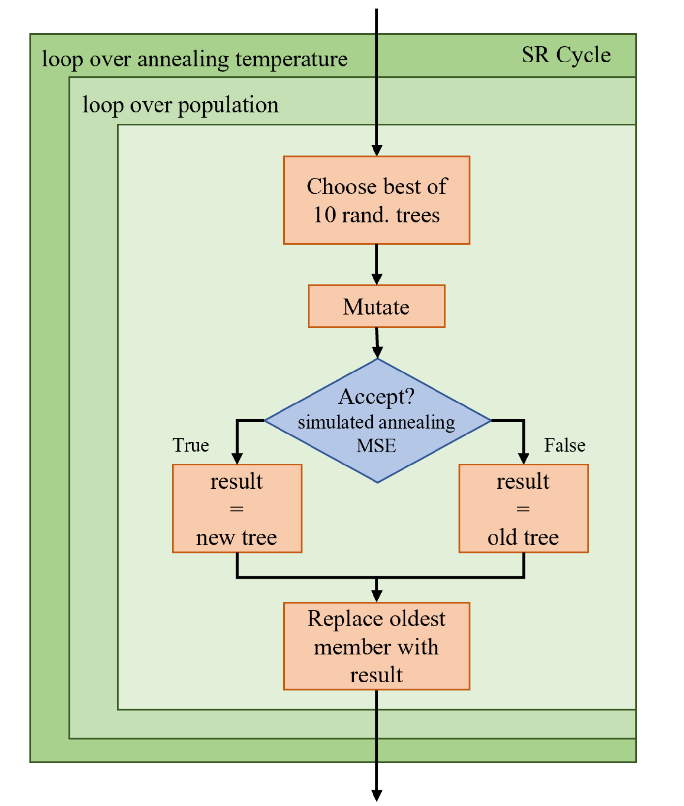
Figure 72: Illustration of the PySR algorithm.

The approximate parton-level description of the score suggests that it should be possible to derive a closed formula in terms of the usual phase space observables. As the numerical starting point we use an event generator like Madgraph to generate a dataset of score values over phase space. Extracting formulas from numerical data is called symbolic regression. The standard application of symbolic regression is in combination with a neural network, where a complex dataset is first described by a neural network, extracting its main feature and providing a fast and numerical powerful surrogate. This neural network is then transformed into approximate formulas. In our case, we directly approximate the numerically encoded score of Eq.(5.64) with compact formulas.

The public tool PySR uses a genetic algorithm to find a symbolic expression for a numerically defined function in terms of pre-defined variables. Its population consists of symbolic expressions, which are encoded as trees and consist of nodes which can either be an operand or an operator function. The operators we need are addition, subtraction, multiplication, squaring, cubing and division, possibly sine and cosine. The algorithm is illustrated in Fig. 72. The tree population evolves when new trees are created and old trees are discarded. Such new trees are created through a range of mutation operators, for instance exchanging, adding, or deleting nodes. The figure of merit which we use to evaluate the new trees is the MSE between the score values $t(x_{i}|\theta)$ and the PySR approximation $g_{i}$, as defined in Eq.(1.22)

$$\text{MSE}\sim\sum_{i}\left[g(x_{i})-t(x_{i}|\theta)\right]^{2}\;,$$ (5.65)

Unlike for a network training we do not want an arbitrarily complex and powerful formula, so we balance the MSE with the number of nodes a complexity measure. The PySR figure of merit is then defined with the additional parsimony parameter through the regularized form

$$\boxed{\text{MSE}^{*}=\text{MSE}+\text{parsimony}\cdot\#_{\text{nodes}}}\;.$$ (5.66)

This combination will automatically find a good compromise between precision and complexity.

Simulated annealing is a standard minimum finder algorithm. Its key feature is a temperature $T$ which allows the algorithm to sample widely in the beginning and then focus on a local minimum. It accepts a mutation of a tree with the probability

$$p=\min\left[\exp\left(-\frac{1}{T}\;\frac{\text{MSE}^{*}_{\text{new}}-\text{MSE}^{*}_{\text{old}}}{\text{MSE}^{*}_{\text{old}}}\right),1\right]\;.$$ (5.67)

If the new tree is better than the old tree, $\text{MSE}^{*}_{\text{new}}<\text{MSE}^{*}_{\text{old}}$, the exponent is larger than zero, and the probability to accept the new tree is one. If the new tree is slightly worse than the old tree, the exponent is smaller than zero, and the algorithm can keep the new tree as an intermediate step to improve the population, but with a finite probability. This probability is rapidly decreased when we dial down the temperature. The output of the PySR algorithm is a set of expressions given by the surviving populations once the algorithm is done. This hall of fame (HoF) depends on the MSE balanced by the number of nodes. If we are really interested in the approximate function. we need to supplement PySR with an optimization fit of all parameters in the HoF functions using the whole data set. Such a fit is too slow to be part of the actual algorithm, but we need it for the final form of the analytic score and for the uncertainties on this form.

There are cases where optimal observables or scores are used for instance by ATLAS to test fundamental properties of their datasets. One such fundamental question is the CP-symmetry of the $VVH$ vertex, which can for instance be tested in weak boson fusion Higgs production. It turns out that for this application we know the functional form of the score at leading order and at the parton level, so we can compare it to the PySR result going beyond these simple approximations. The signal process we need to simulate is

$$pp\to Hjj\;.$$ (5.68)

To define an optimal observable we choose the specific CP-violating operator at dimension six, in analogy to Eq.(5.53),

$$\mathscr{L}=\mathscr{L}_{\text{SM}}+\frac{f_{W\widetilde{W}}}{\Lambda^{2}}\mathcal{O}_{W\widetilde{W}}\qquad\text{with}\qquad\mathcal{O}_{W\widetilde{W}}=-(\phi^{\dagger}\phi)\;\widetilde{W}_{\mu\nu}^{k}W^{\mu\nu k}\;.$$ (5.69)

We know that the signed azimuthal angle between the tagging jets $\Delta\phi$ is the appropriate genuine CP-odd observable. This observable has the great advantage that it is independent of the Higgs decay channels and does not involve reconstructing the Higgs kinematics. In Fig. 73 we show the effect of this operator on the WBF kinematics. First, the asymmetric form of $\Delta\phi$ can most easily be exploited through an asymmetry measurement. Second, the additional momentum dependence of $\mathcal{O}_{W\widetilde{W}}$ leads to harder tagging jets This is unrelated to CP-violation, and we have seen similar effects in Sec. 5.3.1. Finally, there is no effect on the jet rapidities.

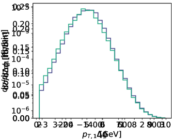
Figure 73: Kinematic distributions for the two tagging jets in WBF Higgs production at parton level for two Wilson coefficients $f_{W\widetilde{W}}$.

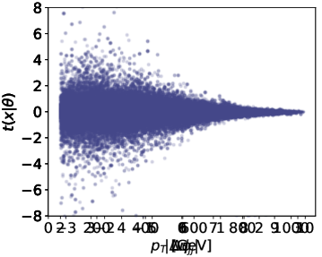
Figure 74: Score for simplified WBF Higgs production at parton level and with $f_{W\widetilde{W}}=0$. The kinematic observables correspond to Fig. 73.

For the leading partonic contribution to $WW$-fusion, $ud\to Hdu$ we can compute the score at the Standard Model point,

$$t(x|f_{W\widetilde{W}}=0)\approx-\frac{8v^{2}}{m_{W}^{2}}\frac{(k_{d}k_{u})+(p_{u}p_{d})}{(p_{d}p_{u})(k_{u}k_{d})}\;\epsilon_{\mu\nu\rho\sigma}\;k_{d}^{\mu}k_{u}^{\nu}p_{d}^{\rho}p_{u}^{\sigma}\;,$$ (5.70)

where $k_{u,d}$ are the incoming and $p_{u,d}$ the outgoing quark momenta. We can assign the incoming momenta to a positive and negative hemisphere, $k_{\pm}=(E_{\pm},0,0,\pm E_{\pm})$, do the same for the outgoing momenta $p_{\pm}$, and then find in terms of the signed azimuthal separation

$$t(x|f_{W\widetilde{W}}=0)\approx-\frac{8v^{2}}{m_{W}^{2}}\frac{2E_{+}E_{-}+(p_{+}p_{-})}{(p_{+}p_{-})}p_{T+}p_{T-}\;\sin\Delta\phi\;.$$ (5.71)

The dependence $t\propto\sin\Delta\phi$ reflects the CP-sensitivity while the prefactor $t\propto p_{T+}p_{T-}$ reflects the dimension-6 origin.

compl	dof	function	MSE
3	1	$a\,\Delta\phi$	$1.30\cdot 10^{-1}$
4	1	$\sin(a\Delta\phi)$	$2.75\cdot 10^{-1}$
5	1	$a\Delta\phi x_{p,1}$	$9.93\cdot 10^{-2}$
6	1	$-x_{p,1}\sin(\Delta\phi+a)$	$1.90\cdot 10^{-1}$
7	1	$(-x_{p,1}-a)\sin(\sin(\Delta\phi))$	$5.63\cdot 10^{-2}$
8	1	$(a-x_{p,1})x_{p,2}\sin(\Delta\phi)$	$1.61\cdot 10^{-2}$
14	2	$x_{p,1}(a\Delta\phi-\sin(\sin(\Delta\phi)))(x_{p,2}+b)$	$1.44\cdot 10^{-2}$
15	3	$-(x_{p,2}(a\Delta\eta^{2}+x_{p,1})+b)\sin(\Delta\phi+c)$	$1.30\cdot 10^{-2}$
16	4	$-x_{p,1}(a-b\Delta\eta)(x_{p,2}+c)\sin(\Delta\phi+d)$	$8.50\cdot 10^{-3}$
28	7	$(x_{p,2}+a)(bx_{p,1}(c-\Delta\phi)$	$8.18\cdot 10^{-3}$
		$\;\;-x_{p,1}(d\Delta\eta+ex_{p,2}+f)\sin(\Delta\phi+g))$

Table 5: Score hall of fame for simplified WBF Higgs production with $f_{W\widetilde{W}}=0$, including a optimization fit.

For small deviations from the CP-conserving Standard Model we show the dependence on the score in Fig. 74. The kinematic observables are the same as in Fig. 73, and we see how $f_{W\widetilde{W}}>0$ moves events from $\Delta\phi>0$ to $\Delta\phi<0$. The dependence on $p_{T,1}$ indicates large absolute values of the score for harder events, which will boost the analysis when correlated with $\Delta\phi$. The dependence on $\Delta\eta$ is comparably mild. To encode this score dependence in a formula we use PySR on the observables

$$\left\{\;x_{p,1},\;x_{p,2},\;\Delta\phi,\;\Delta\eta\;\right\}\qquad\text{with}\qquad x_{p,j}=\frac{p_{T,j}}{m_{H}}\;.$$ (5.72)

In Tab. 5 we show the results, alongside the improvement in the MSE. Starting with the leading dependence on $\Delta\phi$, PySR needs 8 nodes with one free parameter to derive $t\approx p_{T,1}p_{T,2}\sin\Delta\phi$. Beyond this point, adding $\Delta\eta$ to the functional form leads to a further improvement with a 4-parameter description and 16 nodes. The corresponding formula for the score is

$$t(x_{p,1},x_{p,2},\Delta\phi,\Delta\eta|f_{W\widetilde{W}}=0)=-x_{p,1}\left(x_{p,2}+c\right)\left(a-b\Delta\eta\right)\sin(\Delta\phi+d)$$

$$\quad\text{with}\quad a=1.086(11)\quad b=0.10241(19)\quad c=0.24165(20)\quad d=0.00662(32)\;.$$ (5.73)

The numbers in parentheses give the uncertainty from the optimization fit. While $d$ comes out different from zero, it is sufficiently small to confirm the scaling $t\propto\sin\Delta\phi$. Similarly, the dependence on the rapidity difference $\Delta\eta$ is suppressed by $b/a\sim 0.1$. This simple picture will change when we move away from the Standard Model and evaluate the score are finite $f_{W\widetilde{W}}$. However, for this case we neither have a reference results nor an experimental hint to assume such CP-violation in the $HVV$ interaction.

Until now, we have used PySR to extract the score at parton level. The obvious question is what happens when we add a fast detector simulation to the numerical description of the score. To extract the (joint) score from the Madgraph event samples we can use MadMiner. In general, detector effects will mostly add noise to the data, which does affect the PySR convergence. We find the same formulas as without detector effects, for instance the 4-parameter formula of Eq.(5.73), but with different parameters,

$$t(x_{p,1},x_{p,2},\Delta\phi,\Delta\eta|f_{W\widetilde{W}}=0)=-x_{p,1}\left(x_{p,2}+c\right)\left(a-b\Delta\eta\right)\sin(\Delta\phi+d)$$

$$\quad\text{with}\quad a=0.9264(20)\quad b=0.08387(35)\quad c=0.3542(20)\quad d=0.00911(67)\;.$$ (5.74)

The absolute differences are small, even though the pull for instance of $c$ exceeds 100. Still, $d\ll 1$ ensures $t\propto\sin\Delta\phi$ also after detector effects, and $b/a\ll 1$ limits the impact of the rapidity observable. Indeed, detector effects do not introduce a significant bias to the extracted score function.

Figure 75: Projected exclusion limits assuming $f_{W\widetilde{W}}=0$ for different (optimal) observables. The Sally network uses $p_{T_{1}}$, $p_{T_{2}}$, $\Delta\phi$ and $\Delta\eta$, Sally full uses 18 kinematic variables.

Finally, we can switch from the $\text{MSE}^{*}$ figure of merit something more realistic, for instance the expected reach of the different approximations in an actual analysis. To benchmark the reach we can compute the log-likelihood distributions and extract the $p$-value for an assumed $f_{W\widetilde{W}}=0$ including detector effects and for an integrated Run 2 LHC luminosity of $139~{}\text{fb}^{-1}$. The analytic functions we use from the HoF in Fig. 5 are

$$a_{1}p_{T,1}p_{T,2}\qquad\qquad a_{2}\sin\Delta\phi\qquad\qquad a_{3}p_{T,1}p_{T,2}\sin\Delta\phi\;.$$ (5.75)

The first is just wrong and does not probe CP-violation at all. The second taylors the proper results for small azimuthal angles, which does appear justified looking at Fig. 73. The third function is what we expect from the parton level. We compare these three results to the Sally method using the four PySR observables in Eq.(5.72), and using the full set of 18 observables. All exclusion limits are shown in Fig. 75. Indeed, for all score approximations the likelihood follows a Gaussian shape. Second, we find that beyond the minimal reasonable form $ap_{T1}p_{T2}\sin\Delta\phi$ there is only very little improvement in the expected LHC reach for the moderate assumed luminosity.

This application of symbolic regression confirms our hope that we can use modern numerical methods to reverse the general shift from formulas to numerically encoded expressions. In the same spirit as using perturbative QCD we find that symbolic regression provides us with useful and correct approximate formulas, and formulas are the language of physics. The optimal observable for CP-violation is the first LHC-physics formula re-derived using modern machine learning, and at least for Run 2 statistics it can be used in experiment without any loss in performance. However, when analyszing more data we have to extract a more precise formula, again a situation which is standard in physics, where most of our simple formulas rely on a taylor series or a perturbative expansion.

With this appliation we are at the end of our tour of modern machine learning and its LHC applications. We have established neural networks as extremely powerful numerical tools, which are not black boxes, but offer a lot of control. First, an appropriate loss function tells us exactly what the network training is trying to achieve. Second, neural network output comes with an error bar, in some cases like NNPDF even with a comprehensive uncertainty treatment. And, finally, trained neural networks can be transformed into formulas. Given what we can do with modern machine learning at the LHC, there is no excuse to not play with them as new and exciting tools. What we have not talked about is the unifying power of data science and machine learning for the diverging fields of particle theory and particle experiment — to experience this, you will have to come to a conference like ML4Jets or a workshop like Hammers and Nails and watch for yourselves.

References

- [1] M. Feickert and B. Nachman, A Living Review of Machine Learning for Particle Physics, arXiv:2102.02770 [hep-ph].
- [2] ATLAS, G. Aad et al., Expected Performance of the ATLAS Experiment - Detector, Trigger and Physics, arXiv:0901.0512 [hep-ex].
- [3] T. Plehn, Lectures on LHC Physics, Lect. Notes Phys. 844 (2012) 1, arXiv:0910.4182 [hep-ph].
- [4] A. Butter, T. Plehn, S. Schumann, et al., Machine Learning and LHC Event Generation, arXiv:2203.07460 [hep-ph].
- [5] A. Biekötter, F. Keilbach, R. Moutafis, T. Plehn, and J. Thompson, Tagging Jets in Invisible Higgs Searches, SciPost Phys. 4 (2018) 6, 035, arXiv:1712.03973 [hep-ph].
- [6] B. P. Roe, H.-J. Yang, J. Zhu, Y. Liu, I. Stancu, and G. McGregor, Boosted decision trees, an alternative to artificial neural networks, Nucl. Instrum. Meth. A 543 (2005) 2-3, 577, arXiv:physics/0408124.
- [7] Y. Gal, Uncertainty in Deep Learning. PhD thesis, Cambridge, 2016.
- [8] G. Kasieczka, M. Luchmann, F. Otterpohl, and T. Plehn, Per-Object Systematics using Deep-Learned Calibration, SciPost Phys. 9 (2020) 089, arXiv:2003.11099 [hep-ph].
- [9] J. Aylett-Bullock, S. Badger, and R. Moodie, Optimising simulations for diphoton production at hadron colliders using amplitude neural networks, JHEP 08 (2021) 066, arXiv:2106.09474 [hep-ph].
- [10] S. Badger, A. Butter, M. Luchmann, S. Pitz, and T. Plehn, Loop Amplitudes from Precision Networks, arXiv:2206.14831 [hep-ph].
- [11] S. Forte and S. Carrazza, Parton distribution functions, arXiv:2008.12305 [hep-ph].
- [12] NNPDF, R. D. Ball et al., The path to proton structure at 1% accuracy, Eur. Phys. J. C 82 (2022) 5, 428, arXiv:2109.02653 [hep-ph].
- [13] S. Carrazza and J. Cruz-Martinez, Towards a new generation of parton densities with deep learning models, Eur. Phys. J. C 79 (2019) 8, 676, arXiv:1907.05075 [hep-ph].
- [14] L. de Oliveira, M. Kagan, L. Mackey, B. Nachman, and A. Schwartzman, Jet-images — deep learning edition, JHEP 07 (2016) 069, arXiv:1511.05190 [hep-ph].
- [15] G. Kasieczka, T. Plehn, M. Russell, and T. Schell, Deep-learning Top Taggers or The End of QCD?, JHEP 05 (2017) 006, arXiv:1701.08784 [hep-ph].
- [16] S. Macaluso and D. Shih, Pulling Out All the Tops with Computer Vision and Deep Learning, JHEP 10 (2018) 121, arXiv:1803.00107 [hep-ph].
- [17] A. Butter et al., The Machine Learning landscape of top taggers, SciPost Phys. 7 (2019) 014, arXiv:1902.09914 [hep-ph].
- [18] L. Benato et al., Shared Data and Algorithms for Deep Learning in Fundamental Physics, Comput. Softw. Big Sci. 6 (2022) 1, 9, arXiv:2107.00656 [cs.LG].
- [19] S. Bollweg, M. Haußmann, G. Kasieczka, M. Luchmann, T. Plehn, and J. Thompson, Deep-Learning Jets with Uncertainties and More, SciPost Phys. 8 (2020) 1, 006, arXiv:1904.10004 [hep-ph].
- [20] S. Diefenbacher, H. Frost, G. Kasieczka, T. Plehn, and J. M. Thompson, CapsNets Continuing the Convolutional Quest, SciPost Phys. 8 (2020) 023, arXiv:1906.11265 [hep-ph].
- [21] A. Butter, G. Kasieczka, T. Plehn, and M. Russell, Deep-learned Top Tagging with a Lorentz Layer, SciPost Phys. 5 (2018) 3, 028, arXiv:1707.08966 [hep-ph].
- [22] H. Qu and L. Gouskos, ParticleNet: Jet Tagging via Particle Clouds, Phys. Rev. D 101 (2020) 5, 056019, arXiv:1902.08570 [hep-ph].
- [23] B. M. Dillon, G. Kasieczka, H. Olischlager, T. Plehn, P. Sorrenson, and L. Vogel, Symmetries, Safety, and Self-Supervision, arXiv:2108.04253 [hep-ph].
- [24] V. Mikuni and F. Canelli, Point cloud transformers applied to collider physics, Mach. Learn. Sci. Tech. 2 (2021) 3, 035027, arXiv:2102.05073 [physics.data-an].
- [25] P. T. Komiske, E. M. Metodiev, and J. Thaler, Energy Flow Networks: Deep Sets for Particle Jets, JHEP 01 (2019) 121, arXiv:1810.05165 [hep-ph].
- [26] E. M. Metodiev, B. Nachman, and J. Thaler, Classification without labels: Learning from mixed samples in high energy physics, JHEP 10 (2017) 174, arXiv:1708.02949 [hep-ph].
- [27] B. M. Dillon, T. Plehn, C. Sauer, and P. Sorrenson, Better Latent Spaces for Better Autoencoders, SciPost Phys. 11 (2021) 061, arXiv:2104.08291 [hep-ph].
- [28] B. M. Dillon, L. Favaro, T. Plehn, P. Sorrenson, and M. Krämer, A Normalized Autoencoder for LHC Triggers, arXiv:2206.14225 [hep-ph].
- [29] A. Butter, T. Plehn, and R. Winterhalder, How to GAN LHC Events, SciPost Phys. 7 (2019) 6, 075, arXiv:1907.03764 [hep-ph].
- [30] A. Butter, S. Diefenbacher, G. Kasieczka, B. Nachman, and T. Plehn, GANplifying event samples, SciPost Phys. 10 (2021) 6, 139, arXiv:2008.06545 [hep-ph].
- [31] A. Butter, T. Plehn, and R. Winterhalder, How to GAN Event Subtraction, SciPost Phys. Core 3 (2020) 009, arXiv:1912.08824 [hep-ph].
- [32] M. Backes, A. Butter, T. Plehn, and R. Winterhalder, How to GAN Event Unweighting, SciPost Phys. 10 (2021) 4, 089, arXiv:2012.07873 [hep-ph].
- [33] F. A. Di Bello, S. Ganguly, E. Gross, M. Kado, M. Pitt, L. Santi, and J. Shlomi, Towards a Computer Vision Particle Flow, Eur. Phys. J. C 81 (2021) 2, 107, arXiv:2003.08863 [physics.data-an].
- [34] P. Baldi, L. Blecher, A. Butter, J. Collado, J. N. Howard, F. Keilbach, T. Plehn, G. Kasieczka, and D. Whiteson, How to GAN Higher Jet Resolution, arXiv:2012.11944 [hep-ph].
- [35] M. Bellagente, M. Haußmann, M. Luchmann, and T. Plehn, Understanding Event-Generation Networks via Uncertainties, arXiv:2104.04543 [hep-ph].
- [36] B. Stienen and R. Verheyen, Phase space sampling and inference from weighted events with autoregressive flows, SciPost Phys. 10 (2021) 2, 038, arXiv:2011.13445 [hep-ph].
- [37] A. Butter, T. Heimel, S. Hummerich, T. Krebs, T. Plehn, A. Rousselot, and S. Vent, Generative Networks for Precision Enthusiasts, arXiv:2110.13632 [hep-ph].
- [38] E. Bothmann, T. Janßen, M. Knobbe, T. Schmale, and S. Schumann, Exploring phase space with Neural Importance Sampling, SciPost Phys. 8 (2020) 4, 069, arXiv:2001.05478 [hep-ph].
- [39] M. Paganini, L. de Oliveira, and B. Nachman, CaloGAN : Simulating 3D high energy particle showers in multilayer electromagnetic calorimeters with generative adversarial networks, Phys. Rev. D97 (2018) 1, 014021, arXiv:1712.10321 [hep-ex].
- [40] C. Krause and D. Shih, CaloFlow: Fast and Accurate Generation of Calorimeter Showers with Normalizing Flows, arXiv:2106.05285 [physics.ins-det].
- [41] C. Krause and D. Shih, CaloFlow II: Even Faster and Still Accurate Generation of Calorimeter Showers with Normalizing Flows, arXiv:2110.11377 [physics.ins-det].
- [42] A. Andreassen, P. T. Komiske, E. M. Metodiev, B. Nachman, and J. Thaler, OmniFold: A Method to Simultaneously Unfold All Observables, Phys. Rev. Lett. 124 (2020) 18, 182001, arXiv:1911.09107 [hep-ph].
- [43] M. Bellagente, A. Butter, G. Kasieczka, T. Plehn, A. Rousselot, R. Winterhalder, L. Ardizzone, and U. Köthe, Invertible Networks or Partons to Detector and Back Again, SciPost Phys. 9 (2020) 074, arXiv:2006.06685 [hep-ph].
- [44] S. Bieringer, A. Butter, T. Heimel, S. Höche, U. Köthe, T. Plehn, and S. T. Radev, Measuring QCD Splittings with Invertible Networks, SciPost Phys. 10 (2021) 6, 126, arXiv:2012.09873 [hep-ph].
- [45] J. Brehmer, K. Cranmer, G. Louppe, and J. Pavez, A Guide to Constraining Effective Field Theories with Machine Learning, Phys. Rev. D 98 (2018) 5, 052004, arXiv:1805.00020 [hep-ph].
- [46] J. Brehmer, F. Kling, I. Espejo, and K. Cranmer, MadMiner: Machine learning-based inference for particle physics, Comput. Softw. Big Sci. 4 (2020) 1, 3, arXiv:1907.10621 [hep-ph].
- [47] J. Brehmer, S. Dawson, S. Homiller, F. Kling, and T. Plehn, Benchmarking simplified template cross sections in production, JHEP 11 (2019) 034, arXiv:1908.06980 [hep-ph].
- [48] A. Hallin, J. Isaacson, G. Kasieczka, C. Krause, B. Nachman, T. Quadfasel, M. Schlaffer, D. Shih, and M. Sommerhalder, Classifying Anomalies THrough Outer Density Estimation (CATHODE), arXiv:2109.00546 [hep-ph].
- [49] G. Kasieczka et al., The LHC Olympics 2020 a community challenge for anomaly detection in high energy physics, Rept. Prog. Phys. 84 (2021) 12, 124201, arXiv:2101.08320 [hep-ph].