Implementation of an
Oracle-Structured Bundle Method
for Distributed Optimization

Abstract

We consider the problem of minimizing a function that is a sum of convex agent functions plus a convex common public function that couples them. The agent functions can only be accessed via a subgradient oracle; the public function is assumed to be structured and expressible in a domain specific language (DSL) for convex optimization. We focus on the case when the evaluation of the agent oracles can require significant effort, which justifies the use of solution methods that carry out significant computation in each iteration. To solve this problem we integrate multiple known techniques (or adaptations of known techniques) for bundle-type algorithms, obtaining a method which has a number of practical advantages over other methods that are compatible with our access methods, such as proximal subgradient methods. First, it is reliable, and works well across a number of applications. Second, it has very few parameters that need to be tuned, and works well with sensible default values. Third, it typically produces a reasonable approximate solution in just a few tens of iterations. This paper is accompanied by an open-source implementation of the proposed solver, available at https://github.com/cvxgrp/OSBDO.

1 Oracle-structured distributed optimization

1.1 Oracle-structured optimization problem

We consider the optimization problem

$$\begin{array}[]{ll}\mbox{minimize}&h(x)=f(x)+g(x),\end{array}$$ (1)

with variable $x\in{\mbox{\bf R}}^{n}$, where $f,g:{\mbox{\bf R}}^{n}\to{\mbox{\bf R}}\cup\{\infty\}$ are the oracle and structured objective functions, respectively. We assume the problem has an optimal point $x^{\star}$, and we denote the optimal value of the problem (1) as $h^{\star}=h(x^{\star})$. We use infinite values of $f$ and $g$ to encode constraints or the domains, with $\mathop{\bf dom}f=\{x\in{\mbox{\bf R}}^{n}\mid f(x)<\infty\}$ and similarly for $g$. We assume that $\mathop{\bf dom}f\supseteq\mathop{\bf dom}g\neq\emptyset$, i.e., every point in the domain of $g$ is in the domain of $f$, and $g$ has at least one point in its domain.

The oracle objective function.

We assume that the oracle function $f$ is block separable,

$$f(x)=\sum_{i=1}^{M}f_{i}(x_{i}),\quad x=(x_{1},\ldots,x_{M}),$$

with $f_{i}:{\mbox{\bf R}}^{n_{i}}\to{\mbox{\bf R}}\cup\{\infty\}$ closed convex, where $n_{1}+\cdots+n_{M}=n$. We refer to $x_{i}$ as the variable and $f_{i}$ as the objective function of agent $i$. Our access to $f_{i}$ is only via an oracle that evaluates $f_{i}(x_{i})$ and a subgradient $q_{i}\in\partial f_{i}(x_{i})$ at any point $x_{i}\in\mathop{\bf dom}f_{i}$.

The structured objective function.

We assume the structured function $g$ is closed convex. While $f$ is block separable, $g$ (presumably) couples the block variables $x_{1},\ldots,x_{M}$. We assume that $g$ is given in a structured form, using the language of Nesterov, which means we have a complete description of it. We assume that we can minimize $g$ plus some additional structured function of $x$. As a practical matter this might mean that $g$ is expressed in a domain-specific language (DSL) for convex optimization, such as CVXPY [DB16, AVDB18], based on disciplined convex programming (DCP) [GBY06].

Example.

Problem (1) is very general, and includes as special cases many convex optimization problems arising in applications. To give a simple and specific example, it includes the so-called consensus problem [BPC11, Ch. 7],

$$\begin{array}[]{ll}\mbox{minimize}&\sum_{i=1}^{M}f_{i}(x_{i})\\ \mbox{subject to}&x_{1}=\cdots=x_{M},\end{array}$$

where $x_{i}\in{\mbox{\bf R}}^{p}$ are the variables, and $f_{i}$ are given convex functions. We put this in the form (1) with $n_{i}=p$, $n=Mp$, $x=(x_{1},\ldots,x_{M})$, and

$$g(x)=\left\{\begin{array}[]{ll}0&x_{1}=\cdots=x_{M}\\ \infty&\mbox{otherwise},\end{array}\right.$$

the indicator function of the consensus constraint $x_{1}=\cdots=x_{M}$.

Optimality condition.

The optimality condition for problem (1) is: $x$ is optimal if and only if

$$\partial h(x)=\partial f(x)+\partial g(x)\ni 0,$$ (2)

where $\partial h(x)$ denotes the subdifferential of $h$ at $x$. In some applications we may be interested in finding a subgradient $q^{\star}\in\partial f(x^{\star})$ for which $-q^{\star}\in\partial g(x^{\star})$. Such a subgradient can sometimes be interpreted as a vector of optimal prices. The method we describe in this paper will also compute (an estimate of) $q^{\star}$.

Our focus.

We seek an algorithm that solves the distributed oracle-structured problem (1), respecting our access assumptions. Several generic methods can be used, such as proximal subgradient methods or their accelerated extensions, described below. Most research on methods for the composite minimization problem focus on the case where $f$ is differentiable and $g$ has a simple, typically analytically computable, proximal operator, and algorithms that involve very minimal computation beyond evaluation of the gradient of $f$ and the proximal operator of $g$, such as a few vector-vector operations. Our focus here, however, is on the case where the agent oracles can be expensive to evaluate, which has several implications. First, it means that we focus on algorithms that in practice find good suboptimal points in relatively few iterations. Second, it justifies algorithms that solve an optimization problem involving $g$ in each iteration, instead of carrying out just a few vector-vector operations.

Our contribution.

Our contribution is to assemble a number of known methods, such as diagonal preconditioning, level bundle methods, and others into an algorithm that works well on a variety of practical problems, with no parameter tuning. By working well, we mean that modest accuracy, say on the order of $1\%$, is achieved typically in tens of iterations. In the language of the bundle method literature, our final algorithm is a disaggregate partially exact bundle method.

Our open-source implementation, along with all data to reproduce all of our numerical experiments, is available at

https://github.com/cvxgrp/OSBDO.

OSBDO stands for oracle-structured bundle distributed optimization.

1.2 Previous and related work

There is a vast literature on general distributed optimization, but fewer authors consider the specific subgradient oracle plus structured function access we consider here. Several general methods can be used to solve the problem (1) using our access methods, including subgradient, cutting-plane, and bundle-type methods.

Subgradient methods.

Subgradient methods were originally developed by Shor and others in the 1970s [Sho12]. Early work that describes subgradients and convex optimization includes [Roc81]. (To use a subgradient-type method for our problem, we would need to compute a subgradient of $g$, which is readily done.) Subgradient methods typically require a large number of iterations, and are employed when the computational cost of each iteration is low, which is not the case in our setting. Subgradient methods also involve many algorithm parameters that must be tuned, such as a step-size sequence. Modern variations include AdaGrad [DHS11], an adaptive subgradient method which shows good practical results in the online learning setting, but for our setting still requires far too many iterations to achieve even modest accuracy.

Proximal subgradient methods.

A closely related method that is better matched to our specific access restrictions is the proximal subgradient method, which in each iteration requires a subgradient of $f$ and an evaluation of the proximal operator of $g$. (This proximal step is readily carried out since $g$ is structured.) Most of the original work on these types of methods focuses on the case where $f$ is differentiable, and the method is called the proximal gradient method. The proximal gradient method can be described as an operator-splitting method [PB⁺14, Ch. 4.2]; some early work includes [Bru75, CR97]. Since then there have been two relevant developments. The papers [Pas79, LM79] handle the case where $f$ is nondifferentiable, and the gradient is replaced with a subgradient, so the method is called the proximal subgradient method. The stochastic case is addressed in [Sch22], where a stochastic proximal subgradient method is developed. Another advance is the development of simple generic acceleration methods, originally introduced by Nesterov [Nes83]. Other work addresses issues such as inexact computation of the proximal operator [BMR03], or inexact computation of the subgradient [BMLRT15]. Proximal gradient and subgradient methods are widely used in different applications; see, e.g., the book [CP11], which covers proximal gradient method applications in signal processing.

Compared to the method we propose, proximal subgradient methods fail to take into account previously evaluated function values and subgradients (other than through their effect on the current iterate), and our ability to build up a model of each agent function separately. These are done in the method we propose, which requires only a modest increase in complexity over evaluating just the proximal operator of $g$, and give substantial improvement in practical convergence.

Cutting-plane methods.

Cutting-plane methods can be traced back to Cheney and Goldstein [CG59] and Kelley’s cutting-plane method [Kel60]. These methods maintain a piecewise affine lower bound or minorant on the objective, and improve it in each iteration using the subgradient and value of the function at the current iterate. Each iteration requires the solution of a linear program (LP), with size that increases with iterations. Cutting-plane methods are extended to handle convex mixed-integer problems in [WP95]. Limited-memory or constraint-dropping versions, that drop terms in the minorant so the LP solved in each iteration does not grow in size, are given in [EM75, DV85]. Constraint dropping for general outer approximation algorithms are also considered in [GP79]. Many other variations on cutting-plane methods have been developed, including the analytic center cutting-plane method introduced by Atkinson and Vaidya [AV95]. A review of cutting-plane methods used in machine learning can be found in [SNW12].

Bundle methods.

Bundle methods are closely related to cutting-plane methods. The first difference is the addition of a stabilization term, among which a proximal regularization term is most common and leads to the so-called proximal bundle method [Kiw90, Fra20]. Typically in each iteration of the proximal bundle method a quadratic program (QP) must be solved. Other stabilization forms include the level bundle method [LNN95, Fra20] and the trust-region bundle method [MHB75, Fra20]. The second difference between cutting-plane and bundle methods is the logic that updates the current point only if a certain sufficient descent condition holds.

Bundle methods were first developed as dual methods in [Lem75] and [Mif77]; the primal form of bundle methods was mainly studied in the 1990s. The first convergence proof for the proximal bundle method is given in [Lem78]. A comprehensive review of the history and development of bundle methods can be found in [HUL96, Ch. XIV,XV]. Later variations of bundle methods include variable metric bundle methods which accumulate second order information about function curvature in the proximal regularization term [Mif96, CF99, LV99, BQ00, HMM04], bundle methods that handle inexact function values or subgradient values [Hin01, Kiw85, Kiw95, Kiw06, HSS16, vABdOS17, LPM18, OS20], bundle methods with semidefinite cutting sets replacing the traditional polyhedral cutting planes [HR00], and bundle methods with generalized stabilization [Kiw99, Fra02, BADF09, FG14b, OS16]. Bundle methods are also widely used in non-convex optimization [SZ92, Kiw96, LV98, FGG04, HMM07].

Incremental bundle methods [ES10] are based on a principle of selectively skipping oracle calls for some agents, while replacing them by an approximation. Essentially, the function is evaluated when lower and upper estimates on function values are not sufficient [AF18]. This setting was analyzed within a framework of inexact oracles [ES10, OSL14, OE15, vAFdO16], i.e., noisy oracles that are “asymptotically exact”. Further, there has been an interest in asynchronous bundle methods as well [IMdO20, Fis22], where the agent oracle calls have varying finite running times.

Our method for parameter discovery relies on a standard level bundle method [LNN95] for a few initial iterations. We then set the value of the proximal parameter to a Lagrange multiplier and proceed with the proximal bundle method. In a separate study, [OS16] propose an algorithm that automatically chooses between proximal and level bundle approaches at every iteration. Another related line of research is based on variable metric bundle methods [Kiw90, LNN95, LS97, Kiw00, RS02a, Fra02, OSL14, AF18]. In general, these approaches are not crafted for solving composite function minimization satisfying our access conditions.

Our setting with difficult-to-evaluate components has been considered in bundle methods before [ES10]. In those studies, the authors use the inexact evaluations to skip the “hard” components. We, on the other hand, focus on exact oracle evaluations or queries for each component $f_{i}$ alongside the structured function $g$, which is known as partially exact bundle method [vABdOS17]. Our structured function $g$ presents a way to incorporate constraints into bundle methods, which has also been considered before [Kiw90].

In our method we disaggregate the minorant of $f$, an idea which has been extensively studied in the prior literature [Fra02, LOP09, FG14b, FG14a, Fra20]. When combined with the structured function $g$, which is not approximated by a minorant but handled exactly, we arrive at what is referred to as a disaggregate partially exact bundle method.

Software packages.

Despite the large literature on related methods, relatively few open-source software packages are available. We found only one open-source implementation of a bundle method that is compatible with our access requirements. BundleMethod.jl [KZNS21] is a Julia package with implementations of proximal bundle method [Kiw90] and trust region bundle method [KPZ19]. We found that in all our examples OSBDO works substantially better.

We also mention here other existing open-source implementations of bundle methods that do not meet our access methods. A Fortran implementation [Mäk03] with Julia interface for multi-objective proximal bundle method [Mäk03, MKW16], available at [Kar16], requires the objective function to have full domain. A Fortran implementation [TVSL10], uses bundle methods for unconstrained regularized risk minimization. A limited memory bundle method [Kar07, HMM07, KM10] is available as a Fortran implementation at [Kar07], solves nonsmooth large-scale minimization problems, either unconstrained [Kar07, HMM07] or bound constrained [KM10]. An unconstrained proximal bundle method [DG21] with Julia implementation is available at [Dí21].

1.3 Outline

We describe our assembled bundle method for oracle-structured distributed optimization in §2. In §3 we take a deeper look at the agent functions $f_{i}$, which often involve additional variables that are optimized by the agent, and not used by the algorithm, which we call private variables. We present several numerical examples in §4. A convergence proof for our algorithm is given in §A.

2 Disaggregate partially exact bundle method

Here we describe our assembled bundle method to solve the oracle-structured distributed optimization problem (1). We use the superscript $k$ to denote a vector or function at iteration $k$, as in $x_{i}^{k}$ or $x^{k}=(x_{1}^{k},\ldots,x_{m}^{k})$, our estimates of $x_{i}^{\star}$ and $x^{\star}$ at iteration $k$. Each iteration involves querying the agent objective functions, i.e., evaluating $f_{i}(\tilde{x}_{i}^{k})$ and a subgradient $q_{i}^{k}\in\partial f_{i}(\tilde{x}_{i}^{k})$ at a query point $\tilde{x}_{i}^{k}$, for $i=1,\ldots,k$, along with some computation that updates the iterates $x^{k}$. (We will describe what the specific query points are later.)

2.1 Minorants

The basic idea in a bundle or cutting-plane method is to maintain and refine a minorant of each agent function, denoted $\hat{f}_{i}^{k}:{\mbox{\bf R}}^{n_{i}}\to{\mbox{\bf R}}$. (Minorant means that these functions satisfy $\hat{f}_{i}^{k}(x_{i})\leq f_{i}(x_{i})$ for all $x_{i}\in{\mbox{\bf R}}^{n_{i}}$.) They are constructed from initial (given) minorants $\hat{f}_{i}^{0}$, and evaluations of the value and subgradients in previous iterations, as

$$\hat{f}_{i}^{k+1}(x_{i})=\max\left(\hat{f}_{i}^{k}(x_{i}),~{}f_{i}(\tilde{x}_{i}^{k+1})+(q_{i}^{k+1})^{T}(x_{i}-\tilde{x}_{i}^{k+1})\right),\quad i=1,\ldots,M.$$ (3)

Here we use the basic subgradient inequality

$$f_{i}(\tilde{x}_{i}^{k+1})+(q_{i}^{k+1})^{T}(x_{i}-\tilde{x}_{i}^{k+1})\leq f_{i}(x_{i})$$

for all $x_{i}\in{\mbox{\bf R}}^{n_{i}}$, which shows that the lefthand side, which is an affine function of $x_{i}$, is a minorant of $f_{i}$. We also note that the minorant (3) is tight at $\tilde{x}_{i}^{k+1}$, i.e.,

$$\hat{f}_{i}^{k+1}(\tilde{x}_{i}^{k+1})=f_{i}(\tilde{x}_{i}^{k+1}),\quad i=1,\ldots,M.$$

From these agent objective minorants we obtain a minorant of the oracle objective $f$,

$$\hat{f}^{k+1}(x)=\hat{f}^{k+1}_{1}(x_{1})+\cdots+\hat{f}^{k+1}_{M}(x_{M}),$$ (4)

and in turn, a minorant of $h$,

$$\hat{h}^{k+1}(x)=\hat{f}^{k+1}(x)+g(x).$$ (5)

The minorant of $f$ in (4) is referred to as a disaggregated minorant, to distinguish it from forming a minorant directly of $f$.

Initial minorant.

The simplest initial minorant $\hat{f}_{i}^{0}$ is a constant, a known lower bound on the agent objective $f_{i}(x_{i})$. Later we will see how more sophisticated minorants for the agent objectives can be obtained. With a simple constant initial minorant for each agent, the minorant $\hat{f}^{k}$ is also piecewise affine function, since it is a sum of $m$ terms, each the maximum of $k$ affine functions.

Lower bound on optimal value.

Minorants allow us to compute a lower bound on $h^{\star}$, the optimal value of the problem (1). Since $\hat{h}^{k}$ is a minorant of $h$, we have

$$L^{k}=\min_{x}\hat{h}^{k}(x)\leq h^{\star}.$$ (6)

Evaluating $L^{k}$ involves solving an optimization problem, minimizing $g$ plus the piecewise affine function $\hat{f}^{k}$. Of course $h(x^{k})$ is an upper bound on $h^{\star}$, so we have

$$L^{k}\leq h^{\star}\leq h(x^{k}).$$

Gap-based stopping criterion.

There is a multitude of stopping criteria that have been proposed for bundle methods [LNN95, LS97, LSPR96, Fra20, Lem01, HUL96, HUL13]. Many of them are based on approximately satisfying the optimality conditions. For example, we can terminate when the norm of the aggregate subgradient and aggregate linearization error are both small [LS97, LSPR96, Fra20, HUL96, Ch. XIV]. Stopping can also be done based on the predicted function decrease [HUL96, Fra20], which differs depending on the type of stabilization in the bundle method [HUL96, Ch. XV]. We refer the reader to the books [HUL96, HUL13] for more details on stopping criterion for bundle methods. There are other reasonable choices of stopping criteria, for example based on the minorant error $h(x^{k})-\hat{h}^{k}(\tilde{x}^{k+1})$ and a subgradient of $\hat{h}^{k}$ at $\tilde{x}^{k+1}$ see, e.g., [Lem01, Ch. 5.1].

Since we are in the regime where the agents are expensive to evaluate, solving a minimization problem (6) is not an issue, and especially if it is not done every iteration, i.e., we compute the lower bound $L^{k}$ every few iterations. The lower bound (6) gives us a gap-based stopping criterion. In particular, this stopping criterion was previously used in level bundle methods [LNN95, HUL96, Ch. XIV]. We stop if either the absolute gap is small,

$$h(x^{k})-L^{k}\leq\epsilon^{\text{abs}},$$ (7)

where $\epsilon^{\text{abs}}>0$ is a given absolute gap tolerance, or the relative gap is small,

$$h(x^{k})-L^{k}\leq\epsilon^{\text{rel}}\min\{|h(x^{k})|,|L^{k}|\}\quad\mbox{and}\quad h(x^{k})L^{k}>0,$$ (8)

where $\epsilon^{\text{rel}}>0$ is a given relative gap tolerance. (The sign condition guarantees that $\min\{|h(x^{k})|,|L^{k}|\}\leq|h^{\star}|$.) This guarantees that we terminate with a point $x^{k}$ with objective value that is either within absolute difference $\epsilon^{\text{abs}}$, or within relative distance $\epsilon^{\text{rel}}$, of $h^{\star}$.

For later reference, we define the relative gap as

$$\omega^{k}=\left\{\begin{array}[]{ll}\frac{h(x^{k})-L^{k}}{\min\{|h(x^{k})|,|L^{k}|\}}&h(x^{k})L^{k}>0\\ \infty&\mbox{otherwise}.\end{array}\right.$$ (9)

We define the true relative gap as

$$\omega_{\text{true}}^{k}=\frac{h(x^{k})-h^{\star}}{|h^{\star}|},$$ (10)

for $h^{\star}\neq 0$. The relative gap is an upper bound on the true relative gap, i.e., we have $\omega^{k}\geq\omega_{\text{true}}^{k}$. But $\omega^{k}$ is known at iteration $k$, whereas $\omega_{\text{true}}^{k}$ is not.

2.2 Oracle-structured bundle method

The basic bundle method for (1) is given below. It includes two parameters $\eta$ and $\rho$ (discussed later), and is initialized with an initial guess $x^{0}$ of $x$, and the initial minorants of the agent objective functions $\hat{f}_{i}^{0}$.

• Algorithm 2.1 Bundle method for oracle-structured distributed optimization

  given $x^{0}\in\mathop{\bf dom}h$, $h(x^{0})$, initial minorants $\hat{f}_{i}^{0}$, parameters $\eta\in(0,1)$ and $\rho>0$.
  for $k=0,1,\ldots$
  	1. Check stopping criterion. Quit if (7) or (8) holds.
  	2. Tentative update. $\tilde{x}^{k+1}=\mathop{\rm argmin}_{x}\left(\hat{h}^{k}(x)+(\rho/2)\|x-x^{k}\|_{2}^{2}\right)$.
  		Record $\hat{h}^{k}(\tilde{x}^{k+1})$ and $g(\tilde{x}^{k+1})$.
  	3. Query agents. Evaluate $f_{i}(\tilde{x}_{i}^{k+1})$ and $q_{i}^{k+1}\in\partial f_{i}(\tilde{x}_{i}^{k+1})$, for $i=1,\ldots,M$.
  	4. Compute $h(\tilde{x}^{k+1})=f_{1}(\tilde{x}_{1}^{k+1})+\cdots+f_{M}(\tilde{x}_{M}^{k+1})+g(\tilde{x}^{k+1})$.
  	5. Compute $\delta^{k}=h(x^{k})-\left(\hat{h}^{k}\left(\tilde{x}^{k+1}\right)+(\rho/2)\left\|\tilde{x}^{k+1}-x^{k}\right\|_{2}^{2}\right)$.
  	6. Update iterate. Set $x^{k+1}=\begin{cases}\tilde{x}^{k+1}&h(x^{k})-h\left(\tilde{x}^{k+1}\right)\geq\eta\delta^{k}\\ x^{k}&\text{otherwise}.\end{cases}$
  	7. Update minorants.
  		Update $\hat{f}_{i}^{k+1}$ using (3), for $i=1,\ldots,M$.
  		Update $\hat{f}^{k+1}$ and $\hat{h}^{k+1}$ using (4) and (5).

Comments.

In step 1 we evaluate $L^{k}$, which involves solving an optimization problem, i.e., minimizing $\hat{h}^{k}(x)$. We recognize step 2 as evaluating the proximal operator of $\hat{h}^{k}$ at $x^{k}$ [PB⁺14]. This step also involves solving an optimization problem, minimizing $\hat{h}^{k}(x)$ plus the quadratic (proximal) term $(\rho/2)\|x-x^{k}\|_{2}^{2}$. We note that we always have $\tilde{x}^{k+1}\in\mathop{\bf dom}g\subseteq\mathop{\bf dom}f$, so $h(\tilde{x}^{k+1})$ is always finite. Step 3, the agent query, can be done in parallel across all agents. Steps 4 and 5 involve only simple arithmetic using quantities already computed in steps 2 and 3. Steps 1, 5, and 6 use the quantity $h(x^{k})$, but that has already been computed, since $x^{k}$ is equal to a previous $\tilde{x}^{j}$ for some $j\leq k$, and so was computed in step 4 of a previous iteration.

The substantial computation in each iteration of the bundle method is the evaluation of the lower bound in step 1, evaluating the proximal operator of $\hat{h}$ in step 2, and querying each agent oracle in step 3. The computation of $L^{k}$ in step 1 is only used for the stopping criterion, so this step can be carried out only every few steps, to reduce the average computational burden.

Descent method.

The quantity $\delta^{k}$ computed in step 5 is nonnegative. To see this, we note from step 2 that $x=\tilde{x}^{k+1}$ minimizes $\hat{h}^{k}(x)+(\rho/2)\|x-x^{k}\|_{2}^{2}$, so

$$\begin{array}[]{rcl}\hat{h}^{k}(\tilde{x}^{k+1})+(\rho/2)\|\tilde{x}^{k+1}-x^{k}\|_{2}^{2}&\leq&\hat{h}^{k}(x^{k})+(\rho/2)\|x^{k}-x^{k}\|_{2}^{2}\\ &=&\hat{h}^{k}(x^{k})\\ &=&h(x^{k}),\end{array}$$ (11)

from which $\delta^{k}\geq 0$ follows. From step 6 we see that the bundle method is a descent method, i.e., $h(x^{k+1})\leq h(x^{k})$. More specifically, $h(x^{k+1})<h(x^{k})$ if the tentative step is accepted, i.e., $x^{k+1}=\tilde{x}^{k+1}$, and $h(x^{k+1})=h(x^{k})$ if the tentative step is not accepted, i.e., $x^{k+1}=x^{k}$.

Convergence.

In appendix A for completeness we give a proof that the bundle method converges, i.e., $h(x^{k})\to h^{\star}$ as $k\to\infty$. Convergence proofs for bundle methods have long history, dating back to the 1970s [Lem78].

Choice of parameters.

The bundle method is not particularly sensitive to the choice of $\eta$; the value $\eta=0.01$ works well. The value of $\rho$, however, can have a strong influence on the practical performance of the algorithm. We discuss choices of $\rho$ later in §2.4.

Dual variable.

An estimate of an optimal dual variable $q^{\star}\in\partial f(x^{\star})$ can be found when we compute the lower bound $L^{k}$ in step 1. To do this we compute $L^{k}$ by solving the modified problem

$$\begin{array}[]{ll}\mbox{minimize}&\hat{f}^{k+1}(x)+g(\tilde{x})\\ \mbox{subject to}&\tilde{x}=x,\end{array}$$

with variables $x\in{\mbox{\bf R}}^{n}$ and $\tilde{x}\in{\mbox{\bf R}}^{n}$. (This is the consensus form; see, e.g., [BPC11, Chap. 7].) The optimal dual variable associated with the constraint is our estimate of $q^{\star}$.

2.3 Diagonal preconditioning

Practical convergence of the bundle method is greatly enhanced by diagonal preconditioning. This means that we choose a diagonal matrix $D$ with positive entries, and define the (scaled) variable $\overline{x}=D^{-1}x$. Then we solve the problem (1) with variable $\overline{x}$ and functions

$$\overline{f}(\overline{x})=f(D\overline{x}),\qquad\overline{g}(\overline{x})=g(D\overline{x}).$$

Note that $\overline{g}$ is structured, since $g$ is. We recover the solution of the original problem (1) as $x^{\star}=D\overline{x}^{\star}$.

The idea of preconditioning has a long-standing history dating back to 1845 [Jac45] and is a crucial technique in optimization; see, e.g., [HS⁺52, Sin64, CGM85, NW99, Bra10, TJ16]. It is also closely related to the idea of variable metric methods, where essentially a different (not necessarily diagonal) preconditioning is applied each step. Variable metric bundle methods have been studied in [LS94, BLRS01, HP17]. In contrast to our computationally cheap preconditioning technique, which is computed once before the algorithm starts, existing variable metric bundle methods are considerably more complex [Kiw90, LNN95, LS97, Kiw00, RS02a, Fra02, OSL14, AF18]; in addition, most are not compatible with our specific access conditions.

Given $\overline{x}$, we query agent $i$ and the point $x_{i}=D_{i}\overline{x}_{i}$, where $D_{i}$ is the submatrix of $D$ associated with $x_{i}$. Agent $i$ responds with $f_{i}(x_{i})=\overline{f}_{i}(\overline{x}_{i})$ and $q_{i}\in\partial f_{i}(x_{i})$. The algorithm uses the function value without change, since $f_{i}(x_{i})=\overline{f}_{i}(\overline{x}_{i})$, and the scaled subgradient

$$\overline{q}_{i}=Dq_{i}\in\partial\overline{f}_{i}(\overline{x}_{i}).$$

Diagonal scaling can be thought of as a thin layer or interface between the algorithm, which works with the scaled variable $\overline{x}$ and functions $\overline{f}_{i}$ and $\overline{g}$, and the agents, which work with the original variables $x_{i}$ and the original functions $f_{i}$. In particular, neither the algorithm nor the agents need to know that diagonal scaling is being used, provided the query points and returned subgradients are scaled correctly.

A specific choice for diagonal scaling.

The matrix $D$ scales the original variable. Our goal is to scale the variables so they range over similar intervals, say of width on the order of one. To do this, we assume that we have known lower and upper bound on the entries of $x$,

$$l\leq x\leq u,$$ (12)

where $l<u$. (Presumably these constraints are included in $g$.) With these variable bounds we can choose

$$D=\mathop{\bf diag}(u-l).$$ (13)

The new variable bounds have the form $\overline{l}\leq z\leq\overline{u}$, with $\overline{u}-\overline{l}=\mathbf{1}$, the vector with all entries one.

2.4 Proximal parameter discovery

While the bundle algorithm converges for any positive value of the parameter $\rho$, fast convergence in practice requires a reasonable choice that is somewhat problem dependent; see, e.g., [DG21]. Several schemes can be used to find a good value of $\rho$. In one common scheme $\rho$ is updated in each iteration depending on various quantities computed in the iteration. (As an example of such an adaptive scheme, see [BPC11, §3.4.1].) Another general scheme is to start with some steps that are meant to discover a good value of $\rho$, as in [RS02b]. For both such schemes, we fix $\rho$ after some modest number $K$ of iterations, so our proof of convergence (which assumes a fixed value of $\rho$) still applies. Our experiments suggest that a natural $\rho$-discovery method, described below, works well in practice. The idea of switching between proximal and level bundle methods has been proposed in [OS16]. This method is more complex than our proposed simple approach, which switches just once, after a fixed number of iterations.

For the discovery steps, we modify the update in step 2, where we minimize

$$\hat{h}^{k}(x)+(\rho/2)\|x-x^{k}\|_{2}^{2},$$ (14)

i.e., evaluate the proximal operator of $\hat{h}^{k}$ at $x^{k}$, to solving the closely related problem

$$\begin{array}[]{ll}\mbox{minimize}&(1/2)\|x-x^{k}\|_{2}^{2}\\ \mbox{subject to}&\hat{h}^{k}(x)\leq\eta^{k},\end{array}$$ (15)

where $\eta^{k}\in(L^{k},h(x^{k}))$. (This ensures that the problem is feasible, and that the constraint is tight.) The problem (15) finds the projection of the point $x^{k}$ onto the $\eta^{k}$-sublevel set of the minorant. The idea of projecting onto the sublevel set instead of carrying out an explicit proximal step can be found in, e.g., [Fra20, Ch. 2.3].

It is easy to show that any solution of (15) is also a solution of (14), for some value of $\rho$. Indeed we can find this value as $\rho=1/\lambda$, where $\lambda$ is an optimal dual variable for the constraint in (15). In other words: When we solve (15), we are actually computing the proximal operator, i.e., solving (14), for a value of $\rho$ that we only find after solving it.

Our $\rho$-discovery method uses the update (15) for the first $K=20$ steps, with

$$\eta^{k}=\frac{h(x^{k})+L^{k}}{2}.$$

After $K$ steps, we use the standard update (14) with the value of $\rho$ chosen as the geometric mean of the last $5$ values found during the discovery steps.

2.5 Finite memory

Evidently the optimization problems that must be solved to compute $L^{k}$ in step 1 and $\tilde{x}^{k+1}$ in step 2 grow in size as $k$ increases. A standard method in bundle or cutting-plane type methods is to use a finite memory or constraint dropping version, also known as bundle compression [CL93, OE15]. The essential element that underpins theoretical convergence in compressed bundle methods is aggregate linearization [Kiw83, CL93]. It is given by the linearization of the minorant,

$$l_{i}^{k+1}(x_{i})=\hat{f}_{i}^{k}(\tilde{x}_{i}^{k+1})+(\hat{q}_{i}^{k+1})^{T}(x_{i}-\tilde{x}_{i}^{k+1}),$$

where $\hat{q}_{i}^{k+1}\in\partial\hat{f}_{i}^{k}(\tilde{x}_{i}^{k+1})$. As a result, a finite memory version replaces the minorant (3) with

$$\hat{f}_{i}^{k+1}(x_{i})=\max\left(l_{i}^{k+1}(x_{i}),\max_{j=\max\{0,k-m+2\},\ldots,k}\left(f_{i}(\tilde{x}_{i}^{j+1})+(q_{i}^{j+1})^{T}(x_{i}-\tilde{x}_{i}^{j+1})\right)\right),$$

for all $i=1,\ldots,M$. Thus we use only the last $m-1$ subgradients and values in the minorant, instead of all previous ones with an additional affine term for aggregate linearization. This results in total of $m$ affine functions. For further information on bundle compression, refer to [CL93, Lem01, OE15, Fra20]. Interestingly, the minorant $\hat{f}_{i}^{k+1}(x_{i})$ can be reduced to just two affine pieces. However, in practical applications, a smaller bundle size leads to slower convergence rates [OE15]. (Finite-memory should not be confused with limited-memory, which can refer to a quasi-Newton algorithm that approximates the Hessian using a finite number of function and gradient evaluations.)

With finite memory it is possible that the lower bounds $L^{k}$ are not monotone nondecreasing. In this case we can keep track of the best (i.e., largest) lower bound found so far, for use in our stopping criterion.

3 Agents

In this section we discuss some details of the agent objective functions, and how to compute the value and a subgradient. For simplicity we drop the subscript $i$ that was used denote agent $i$, so in this section, we denote $x_{i}$ as $x$, $f_{i}$ as $f$, $q_{i}$ as $q$, and so on.

Private variables and partial minimization.

In many cases the agent function $f$ is defined via partial minimization, as the optimal value of a problem with variable $x$ and additional variables $z$. Specifically, $f(x)$ is the optimal value of the problem

$$\begin{array}[]{ll}\mbox{minimize}&F_{0}(x,z)\\ \mbox{subject to}&F_{i}(x,z)\leq 0,\quad i=1,\ldots,m,\\ &H_{i}(x,z)=0,\quad i=1,\ldots,p,\end{array}$$

with variable $z$. (In this optimization problem, $x$ is a parameter.) Here $F_{i}$ are jointly convex in $(x,z)$, and $H_{i}$ are jointly affine in $(x,z)$. This is called partial minimization [BV04, §4.1], and defines $f$ that is convex. To evaluate $f$ we must solve a convex optimization problem. We refer to $x$ as the public variable for the agent, and $z$ as its private variable, since its value (or even its existence) is not known outside the agent.

We now explain how to find a subgradient $q\in\partial f(x)$. We solve the equivalent convex problem

$$\begin{array}[]{ll}\mbox{minimize}&F_{0}(\tilde{x},z)\\ \mbox{subject to}&F_{i}(\tilde{x},z)\leq 0,\quad i=1,\ldots,m,\\ &H_{i}(\tilde{x},z)=0,\quad i=1,\ldots,p,\\ &\tilde{x}=x,\end{array}$$

with variables $z$ and $\tilde{x}$. (As in the problem above, $x$ is a parameter in this optimization problem.) We assume that strong duality holds for this problem (which is guaranteed if the stronger form of Slater’s condition holds), with $\nu$ denoting an optimal dual variable for the constraint $\tilde{x}=x$. Then it is easy to show that $q=-\nu$ is a subgradient of $f$ [BDPV22] assuming strong duality holds.

Soft constraints and slack variables.

We assume that the domain of the agent objective function includes the domain of $g$. This is critical since the agents will always be queried at a point $\tilde{x}\in\mathop{\bf dom}g$, and we need the agent objective function to be finite for any such $\tilde{x}$. In some cases this property does not hold for the natural definition of the agent objective function. Here we explain how to modify an original definition of an agent objective function $f$ so that it does.

Let $\tilde{f}$ be the original agent objective function, which does not satisfy $\mathop{\bf dom}\tilde{f}\subseteq\mathop{\bf dom}g$. It is often possible to replace constraints that appear in the original definition of $\tilde{f}$ with soft constraints, that ensure that $\mathop{\bf dom}\tilde{f}\subseteq\mathop{\bf dom}g$ holds.

There is also a generic method that uses slack variables to ensure that $f$ has full domain (which implies the domain condition). We define

$$f(x)=\min_{\tilde{x}}\left(\tilde{f}(\tilde{x})+\lambda\|\tilde{x}-x\|_{1}\right),$$

where $\lambda>0$ is a parameter. This $f$ is convex and has full domain. For $\lambda$ large enough and $x\in\mathop{\bf dom}\tilde{f}$, we have $\tilde{x}=x$. We can think of $\tilde{x}-x$ as a slack variable, used to guarantee that $f(x)$ is defined for all $x$. We interpret $\lambda$ as a penalty for using the slack variable.

4 Examples

In this section we present a number of examples to illustrate our method. There are better methods to solve each of these examples, which exploit the custom structure of the particular problem. Our purpose here is to show that a variety of large-scale practical problems achieve good practical performance, i.e., modest accuracy in some tens of iterations, with OSBDO with default parameters.

We use the default parameters for the first four examples, except that we continue iterations after the algorithm would have terminated with the default tolerances $\epsilon^{\text{abs}}=10^{-3}$ and $\epsilon^{\text{rel}}=10^{-2}$, to show the continued progress. The final subsection gives experimental results for the bundle method with finite memory (described in §2.5).

4.1 Supply chain

Supply chain problems involve the placement and movement of inventory, including sourcing from a supplier and distribution to an end customer. A comprehensive review can be found in [TMAS16]. Here we consider a single commodity network composed of a series of $M$ trans-shipment components. Each of these has a vector $a_{i}$ of (nonnegative) flows into it, and a vector $b_{i}$ of (nonnegative) flows out of it. These are connected in series, with the first trans-shipment component’s output connected to the second component’s input, and so on, so

$$b_{1}=a_{2},~{}\ldots,~{}b_{M-1}=a_{M}.$$ (16)

The vector $a_{1}$ gives the flows into the first trans-shipment component, and $b_{M}$ is the vector of flows out of the last trans-shipment component. This is illustrated in figure 1.

Figure 1: Supply chain consisting of a source (left), a sequence of $M$ trans-shipment components (middle), and a sink (right).

We assume the trans-shipment components are lossless, which means that

$$\mathbf{1}^{T}a_{i}=\mathbf{1}^{T}b_{i},\quad i=1,\ldots,M,$$ (17)

i.e., the total flow of the commodity into each trans-shipment component equals the total flow leaving it.

Each trans-shipment component has a nonnegative objective function $f_{i}(a_{i},b_{i})$ which we interpret as the cost of shipping the commodity from the input flows to the output flows. In addition there is a source (purchase) objective term $\psi^{\text{src}}(a_{1})$, the cost of purchasing the commodity, and a sink (delivery) objective term $\psi^{\text{sink}}(b_{M})$, which we interpret as the negative revenue derived from delivering the commodity. (So we expect that $\psi^{\text{src}}(a_{1})$ is nonnegative, and $\psi^{\text{sink}}(b_{M})$ is nonpositive.)

The overall objective is the total of the trans-shipment costs and the source and sink costs,

$$\psi^{\text{src}}(a_{1})+f_{1}(a_{1},b_{1})+\cdots+f_{M}(a_{M},b_{M})+\psi^{\text{sink}}(b_{M}).$$

Our goal is to choose the input and output flows $a_{i}$ and $b_{i}$, subject to the flow conservation constraints (16), so as to minimize this total objective. We assume $\psi^{\text{src}}$, $\psi^{\text{sink}}$, and all $f_{i}$ are convex, and that $\psi^{\text{src}}$ and $f_{i}$ are nonnegative.

Oracle-structured form.

We put the supply chain problem into the form (1) as follows. We take $x_{i}=(a_{i},b_{i})$ for $i=1,\ldots,M$, with variable range $0\leq x\leq u$, where $u$ is an upper bound on the flows. We take $g$ to be the source and sink objective terms, plus the indicator function of the flow conservation constraints (16), variable ranges, and flow balance (17):

$$g(x)=\left\{\begin{array}[]{ll}\psi^{\text{src}}(a_{1})+\psi^{\text{sink}}(b_{M})&\eqref{e-flow-conserv},~{}\eqref{e-tranship-flow-balance},~{}0\leq x\leq u,\\ \infty&\mbox{otherwise}.\end{array}\right.$$

Roughly speaking, $g(x)$ is the gross negative profit, and $f(x)$ is the total shipping cost.

Our initial minorant is the indicator function of the flow conservation constraint (17), i.e., $0$ if (17) holds and $\infty$ otherwise. Note that this includes the lower bound $0\leq f_{i}(x_{i})$.

Trans-shipment cost.

The trans-shipment cost for agent $i$ is based on a fully bipartite graph, with flow along each edge connecting one of $q_{i}$ inputs to each of $p_{i}$ outputs. We represent the edge flows as $X_{i}\in{\mbox{\bf R}}^{p_{i}\times q_{i}}$, where $a_{i}\in{\mbox{\bf R}}^{q_{i}}$ and $b_{i}\in{\mbox{\bf R}}^{p_{i}}$, and $(X_{i})_{jk}$ is the flow from input $k$ to output $j$.

We assume that each edge has a convex quadratic cost of the form

$$(D_{i})_{jk}(X_{i})_{jk}+(E_{i})_{jk}(X_{i})_{jk}^{2},$$

with $(D_{i})_{jk}\geq 0$, and in addition is capacitated, i.e., $0\leq(X_{i})_{jk}\leq(C_{i})_{jk}$, with $(C_{i})_{jk}\geq 0$. Due to the capacity constraints, the domain condition $\mathop{\bf dom}f_{i}\supseteq\mathop{\bf dom}g$ need not hold, so in addition we include a slack variable. We define $f_{i}(x_{i})$ as the optimal value of the trans-shipment problem

$$\begin{array}[]{ll}\mbox{minimize}&\sum_{j,k}\left((D_{i})_{jk}(X_{i})_{jk}+(E_{i})_{jk}(X_{i})_{jk}^{2}\right)+\lambda\|r\|_{1}\\ \mbox{subject to}&0\leq(X_{i})_{jk}\leq(C_{i})_{jk},\quad j=1,\ldots,p_{i},\quad k=1,\ldots,q_{i}\\ &\sum_{j}(X_{i})_{jk}=(\tilde{a}_{i})_{k},\quad k=1,\ldots,q_{i}\\ &\sum_{k}(X_{i})_{jk}=(\tilde{b}_{i})_{j},\quad j=1,\ldots,p_{i},\\ &(\tilde{a}_{i},\tilde{b}_{i})-r=x_{i},\end{array}$$

with variables $(X_{i})_{jk}$, $\tilde{a}_{i}$, $\tilde{b}_{i}$, and $r$. Here $\lambda$ is a large positive parameter that penalizes using slack variables, i.e., having $\tilde{a}_{i}\neq a_{i}$ or $\tilde{b}_{i}\neq b_{i}$.

To evaluate $f_{i}(x_{i})$ we solve the problem above, which is a convex QP. To obtain a subgradient of $f_{i}$ at $x_{i}$ we use the negative optimal dual variables associated with the last constraint as $q_{i}$.

Source and sink costs.

We take simple linear source and sink costs,

$$\psi^{src}(a_{1})=\alpha^{T}a_{1},\qquad\psi^{sink}(b_{M})=\beta^{T}b_{M},$$

with $\alpha\geq 0$ and $\beta\leq 0$. We can interpret $\alpha_{k}$ as the price of acquiring the commodity at input $k$ of the first trans-shipment component, and $-\beta_{k}$ as the price of selling the commodity at output $k$ of the last trans-shipment component.

Problem instance.

We consider a problem instance with $M=5$ trans-shipment components, and dimensions of $a_{i},b_{i}$ given by

$$(20,30),\quad(30,40),\quad(40,25),\quad(25,35),\quad(35,20).$$

We choose the edge capacities $(C_{i})_{jk}$ from a log normal distribution, with $\log(C_{i})_{jk}\sim\mathcal{N}(0,1)$. From these edge capacities we construct an upper bound on each component of $x_{i}$, as the maximum of the sum of the capacities of all edges that feed the flow variable, and the sum of the capacities of all edges that flow out of it. This gives us our upper bound $u$. The linear cost coefficients $(E_{i})_{jk}$ are log normal, with $\log(E_{i})_{jk}\sim\mathcal{N}(0.07,0.7)$. The quadratic cost coefficients $(D_{i})_{jk}$ are obtained from the capacity and linear cost coefficients as

$$(D_{i})_{jk}=(E_{i})_{jk}/(2(C_{i})_{jk}).$$

The sale prices $\alpha$ are uniform on $[8,10]$ and retail prices $-\beta$ are chosen uniformly on $[10,12]$. The total problem size is $n=300$ public variables (the input and output flows of the trans-shipment components), with an additional $4975$ private variables in the agents (the specific flows along all edges of the trans-shipment components). The overall problem is a QP with $5275$ variables.

Results.

Figure 2 shows the relative gap $\omega^{k}$ and true relative gap $\omega_{\text{true}}^{k}$, versus iterations. With the default stopping criterion parameters the algorithm would have terminated after $80$ iterations, when it can guarantee that it is no more than $1\%$ suboptimal. In fact, it is around $0.3\%$ suboptimal at that point. This is shown as the vertical dashed line in the plot. We can also see that the relative accuracy was in fact better than $1\%$ after only $59$ iterations, but, roughly speaking, we did not know it then.

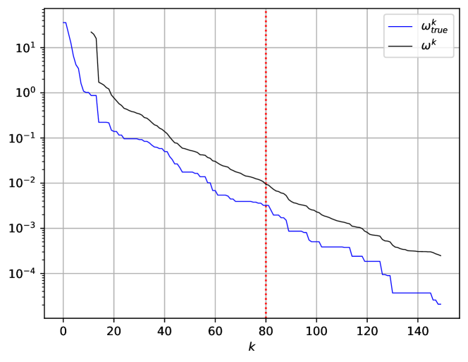
Figure 2: Relative gap and true relative gap versus iterations for supply chain example.

4.2 Resource allocation

Resource allocation problems consider how to allocate a limited amount of several resources to a number of participants in order to optimize some overall objective. This kind of problem arises in communication networks [HL08], urban development [WZX⁺20], cloud computing [CL16], and many others. Various candidate algorithms have been explored to solve this problem, with interesting ones including ant colony algorithm [YW06], genetic algorithm [LZDL05], and a graph-based approach [ZBL⁺21]. In this section, we demonstrate how bundle method can be exploited to address a distributed version of the generic resource allocation problem.

Resource allocation problem.

We consider the optimal allocation of $n$ resources to $N$ participants. We let $r_{i}\in{\mbox{\bf R}}_{+}^{n}$ denote the amounts of the resources allocated to participant $i$, for $i=1,\ldots,N$. The utility derived by participant $i$ is $U_{i}(r_{i})$, where $U_{i}:{\mbox{\bf R}}_{+}^{n}\to{\mbox{\bf R}}$ is a concave nondecreasing utility function. The resource allocation problem is to allocate resources to maximize the total utility subject to a limit on the total resources allocated:

$$\begin{array}[]{ll}\mbox{maximize}&\sum_{i=1}^{N}U_{i}(r_{i})\\ \mbox{subject to}&r_{i}\geq 0,\quad i=1,\ldots,N\\ &\sum_{i=1}^{N}r_{i}\leq R,\end{array}$$

with variables $r_{1},\ldots,r_{N}$, where $R\in{\mbox{\bf R}}_{+}^{n}$ is the total resources to be allocated, i.e., the budget. We denote the optimal value, i.e., the maximum total utility, as a function of $R$ as $U^{\star}(R)$. It is also concave and nondecreasing. When we solve this problem, an optimal dual variable associated with the last (budget) constraint can be interpreted as the prices of the resources.

Distributed resource allocation problem.

We have $M$ groups of participants, each with its own set of participants, resource budget $R_{i}\in{\mbox{\bf R}}_{+}^{n}$, and utility $U^{\star}_{i}(R_{i})$. The distributed resource allocation problem is

$$\begin{array}[]{ll}\mbox{maximize}&\sum_{i=1}^{M}U^{\star}_{i}(R_{i})\\ \mbox{subject to}&R_{i}\geq 0,\quad i=1,\ldots,M\\ &\sum_{i=1}^{M}R_{i}\leq R,\end{array}$$

with variables $R_{1},\ldots,R_{M}$, where $R$ is the total budget of resources. This problem has exactly the same form as the resource allocation problem, but here $U_{i}^{\star}(R_{i})$ is the optimal total utility for group $i$ of participants, whereas in the resource allocation problem, $U_{i}(r_{i})$ is the utility of the single participant $i$.

Oracle-structured form.

Each agent is associated with a group in the distributed resource allocation problem. We take $x_{i}=R_{i}$, the total resource allocated to the participants in group $i$. We take agent objective functions

$$f_{i}(x_{i})=-U_{i}^{\star}(x_{i}),\quad i=1,\ldots,M,$$

the optimal (negative) total utility for its group of participants, given resources $x_{i}$. We take the structured objective function to be

$$g(x)=\left\{\begin{array}[]{ll}0&x_{1}+\cdots+x_{M}\leq R,\quad x_{i}\geq 0,\quad i=1,\ldots,M\\ \infty&\mbox{otherwise}.\end{array}\right.$$

With these agent and structured objectives, the problem (1) is equivalent to the distributed resource allocation problem. The resource allocations to the individual participants within each group are private variables; the public variables are the total resources allocated to each group.

To evaluate $f_{i}(\tilde{x}_{i})$, we solve the resource allocation problem for group $i$. To find a subgradient $q\in\partial f_{i}(\tilde{x}_{i})$, we take the negative of an optimal dual variable in the resource allocation problem, i.e., the negative of the optimal prices. To obtain a range on each variable, we use $0\leq x_{i}\leq R$.

Problem instance.

Our example uses participant utility functions of the form

$$U_{i}(r_{i})=\mathop{\bf geomean}\left(A_{i}r_{i}+b_{i}\right),$$

where $\mathop{\bf geomean}(u)=\left(\prod_{i=1}^{p}u_{i}\right)^{1/p}$ for $u\in{\mbox{\bf R}}_{+}^{p}$ is the geometric mean function. The entries of $A_{i}$ are nonnegative, so $U_{i}$ is concave and nondecreasing. We choose $A_{i}$ to be column sparse, with around $\frac{n}{10}$ columns chosen at random to be nonzero. The nonzero entries in these columns are chosen as uniform on $[0,1]$. We choose entries of $b_{i}$ to be uniform on $[0,\frac{n}{10}]$. The resource budgets $R_{i}$ are chosen from $\log R_{i}\sim\mathcal{N}(\log\frac{n}{10},1)$. The initial minorant is given by

$$\hat{f}^{0}=\sum_{i=1}^{M}\sum_{j=1}^{N_{i}}-\mathop{\bf geomean}(A_{ij}R+b_{ij}),$$

the negative of the utility if all agents were given the full budget of resources.

For the specific instance we consider, we take $n=50$ resources and $M=50$ agents, each of which allocates resources to $N_{i}=10$ participants. (As a single resource allocation problem we would have $50$ resources and $500$ participants.) The utility functions use $p=5$, i.e., each is the geometric mean of $5$ affine functions.

Results.

Figure 3 shows the relative gap $\omega^{k}$ and true relative gap $\omega_{\text{true}}^{k}$ versus iterations. With the default stopping criterion the algorithm would have terminated after $47$ iterations (shown as the vertical dashed line), when it can guarantee that it is no more than $1\%$ suboptimal. In fact, it is around $0.5\%$ suboptimal at that point. We can also see that the relative accuracy was better than $1\%$ after only $33$ iterations.

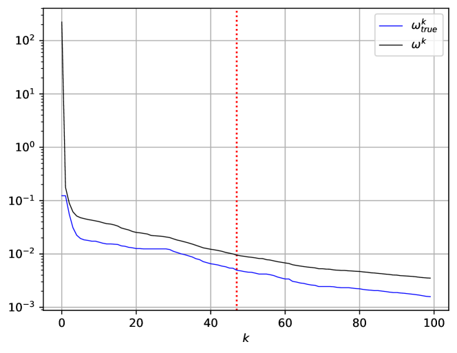
Figure 3: Relative gap and true relative gap versus iterations for resource allocation example.

4.3 Multi-commodity flow

Multi-commodity flow problems involve shipping different commodities on the same network in a way such that the total utility is maximized, while the total flow on each edge stays below its capacity. In [OMV00] authors give a survey of algorithms for this problem. We consider a network defined by a graph with $p$ vertices or nodes and $q$ directed edges, defined by the incidence matrix $A\in{\mbox{\bf R}}^{p\times q}$. The network supports the flow of $M$ different commodities. Each commodity has a source node, denoted $r_{i}\in\{1,\ldots,p\}$, and a sink or destination node, denoted $s_{i}\in\{1,\ldots,p\}$. The flow of commodity $i$ from the source to destination is given by $d_{i}\geq 0$. We let $z_{i}\in{\mbox{\bf R}}_{+}^{q}$ be the vector of flows of commodity $i$ on the edges. Flow conservation is the constraint

$$Az_{i}+d_{i}(e_{r_{i}}-e_{s_{i}})=0,\quad i=1,\ldots,M,$$

where $e_{k}$ denotes the $k$th unit vector, with $(e_{k})_{k}=1$ and $(e_{k})_{j}=0$ for $j\neq k$. Flow conservation requires that the flow is conserved at all nodes, with $d_{i}$ injected at the source node, and $d_{i}$ removed at the sink node. The utility of flow $i$ is $U_{i}(d_{i})$, where $U_{i}$ is a concave nondecreasing function. Our objective is to maximize the total utility $U_{1}(d_{1})+\cdots+U_{M}(d_{M})$.

The total flow on the edges must not exceed the capacities on the edges, given by $c\in{\mbox{\bf R}}_{+}^{q}$, i.e.,

$$z_{1}+\cdots+z_{M}\leq c.$$

(This capacity constraint couples the variables associated with the different commodities.)

The variables in this multi-commodity flow problem are $z_{1},\ldots,z_{M}$ and $d_{1},\ldots,d_{M}$. The data are the incidence matrix $A$, the edge capacities $c$, the commodity source and sink nodes $(r_{i},s_{i})$, and the flow utility functions $U_{i}$.

It will be convenient to work with a form of the problem where we split the capacity on each edge into $M$ different capacities for the different commodities. We take

$$z_{i}\leq c_{i},\quad i=1,\ldots,M,$$

where $c_{1}+\cdots+c_{M}=c$ and $c_{i}\geq 0$ for $i=1,\ldots,M$. We interpret $c_{i}$ as the edge capacity assigned to, or reserved for, commodity $i$. Our multi-commodity flow problem then has the form

$$\begin{array}[]{ll}\mbox{maximize}&U_{1}(d_{1})+\cdots+U_{M}(d_{M})\\ \mbox{subject to}&0\leq z_{i}\leq c_{i},\quad i=1,\ldots,M\\ &Az_{i}+d_{i}(e_{r_{i}}-e_{s_{i}})=0,\quad i=1,\ldots,M\\ &c_{1}+\cdots+c_{M}=c,\quad c_{i}\geq 0,\quad i=1,\ldots,M,\end{array}$$

with variables $z_{i}$, $d_{i}$, and $c_{i}$. This is evidently equivalent to the original multi-commodity flow problem.

Oracle-structured form.

We can put the multi-commodity flow problem into oracle-structured form as follows. We take $x_{i}=c_{i}$, the edge capacity assigned to commodity $i$. We take the range of $x_{i}$ as $0\leq x_{i}\leq c$. We take the agent cost function $f_{i}(x_{i})$ to be the optimal value of the single commodity flow problem (expressed as a minimization problem)

$$\begin{array}[]{ll}\mbox{minimize}&-U_{i}(d_{i})\\ \mbox{subject to}&0\leq z_{i}\leq x_{i}\\ &Az_{i}+d_{i}(e_{r_{i}}-e_{s_{i}})=0,\end{array}$$

with variables $z_{i}$ and $d_{i}$. (Here $x_{i}=c_{i}$ is a parameter.) These functions $f_{i}(x_{i})$ are convex and nonincreasing in $x_{i}$, the capacity assigned to commodity $i$. To evaluate $f_{i}$ we solve the single commodity flow problem above; a subgradient $q_{i}$ is obtained as the negative optimal dual variable associated with the capacity constraint $z_{i}\leq x_{i}$.

We take $g(x)$ to be the indicator function of

$$x_{1}+\cdots+x_{M}=c,\quad x_{i}\geq 0,\quad i=1,\ldots,M$$

(which includes the ranges of $x_{i}$).

All together there are $n=Mq$ variables, representing the allocation of edge capacity to the commodities. There are also $M(q+1)$ private variables, which are the flows for each commodity on each edge and the values of the flows of each commodity.

Problem instance.

We consider an example with $M=10$ commodities, and a graph with $p=100$ nodes and $q=1000$ edges. Edges are generated randomly from pairs of nodes, with an additional cycle passing through all vertices (to ensure that the graph is strongly connected, i.e., there is a directed path from any node to any other). We choose the source-destination pairs $(r_{i},s_{i})$ randomly. We choose capacities $c_{i}$ from a uniform distribution on $[0.2,2]$. The flow utilities $U_{i}$ are linear, i.e., $U_{i}(d_{i})=b_{i}d_{i}$, with $b_{i}$ chosen uniformly on $[0.5,1.5]$. This problem instance has $n=10000$ variables, with an additional $10010$ private variables.

Results.

Figure 4 shows the relative gap $\omega^{k}$ and true relative gap $\omega_{\text{true}}^{k}$ versus iterations. With the default stopping criterion the algorithm would have terminated after $14$ iterations (shown as the vertical dashed line), when it can guarantee that it is no more than $1\%$ suboptimal. In fact, it is around $0.6\%$ suboptimal at that point. We can also see that the relative accuracy was better than $1\%$ after only $13$ iterations.

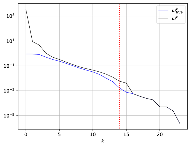
Figure 4: Relative gap and true relative gap for multi-commodity flow example.

4.4 Federated learning

Federated learning refers to distributed machine learning, where agents keep their local data and collaboratively train a model using a distributed algorithm. An overview of the development of federated learning is given in [LSTS20]. In this section we consider the federated learning problem.

We are to fit a model parameter $\theta\in{\mbox{\bf R}}^{d}$ to data that is stored in $M$ locations. Associated with each location is a function $L_{i}:{\mbox{\bf R}}^{d}\to{\mbox{\bf R}}$, where $L_{i}(\theta)$ is the loss for parameter value $\theta$ for the data held at location $i$. We seek $\theta$ that minimizes

$$\sum_{i=1}^{M}L_{i}(\theta)+R(\theta),$$

where $R:{\mbox{\bf R}}^{d}\to{\mbox{\bf R}}\cup\{\infty\}$ is a regularization function. We assume that $L_{i}$ and $R$ are convex, so this fitting problem is convex. In federated learning [KMA⁺21], we solve the fitting problem in a distributed manner, with each location handling its own data.

Oracle-structured form.

We can put the federated learning problem into oracle-structured form by taking $x_{i}$ to be the parameter estimate at location $i$, $f_{i}=L_{i}$, and $g$ the indicator function for consensus plus the regularization,

$$g(x)=\left\{\begin{array}[]{ll}R(x_{1})&x_{1}=\cdots=x_{M}\\ \infty&\mbox{otherwise}.\end{array}\right.$$

Problem instance.

We consider a classification problem with logistic loss function,

$$L_{i}(\theta)=\sum_{j=1}^{n_{i}}\log\left(1+\exp(-v_{ij}u_{ij}^{T}\theta)\right),$$

where $v_{ij}\in\{-1,1\}$ is the label and $u_{ij}\in{\mbox{\bf R}}^{d}$ is the feature value for data point $j$ in location $i$, and $n_{i}$ is the number of data points at location $i$. We use $\ell_{1}$ regularization, i.e., $R(\theta)=\lambda\|\theta\|_{1}$, where $\lambda>0$.

Our example takes parameter dimension $d=500$, $M=10$ locations, and $n_{i}=1000$ data points at each location. In this problem there are no private variables, and the total dimension of $x$ is $n=Md=5000$.

We generate the data points as follows. The entries of $u_{ij}$ are $\mathcal{N}(0,1)$, and we take

$$v_{ij}=\mathop{\bf sign}\left(u_{ij}^{T}\theta^{\mathrm{true}}+z_{ij}\right),$$

where $z_{ij}\sim\mathcal{N}(0,10^{-2})$ and $\theta^{\mathrm{true}}$ is a true value of the parameter, chosen as sparse with around $50$ nonzero entries, each $\mathcal{N}(0,1)$. We choose $\lambda=5$.

Results.

Figure 5 shows the relative gap $\omega^{k}$ and true relative gap $\omega_{\text{true}}^{k}$ versus iterations. With the default stopping criterion the algorithm would have terminated after $53$ iterations (shown as the vertical dashed line), when it can guarantee that it is no more than $1\%$ suboptimal. In fact, it is around $0.3\%$ suboptimal at that point. We can also see that the relative accuracy was better than $1\%$ after only $39$ iterations.

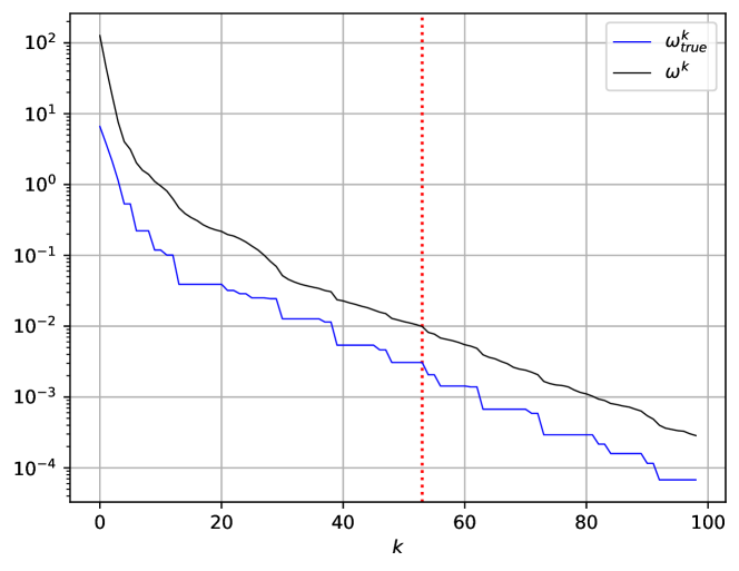
Figure 5: Relative gap and true relative gap versus iterations for federated learning example.

4.5 Finite-memory experiments

In this subsection we present results showing how limiting the memory to various values affects convergence. In many cases, limiting the value to $m=20$ or more has negligible effect. As an example, figure 6 shows the effect on convergence of memory with values $m=20$, $m=30$, $m=50$, and $m=\infty$ for the federated learning problem described above. In this example finite memory has essentially small effect on the convergence.

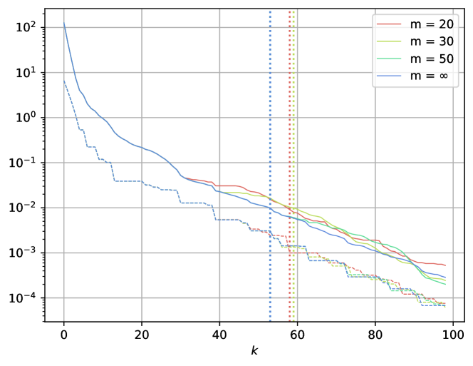
Figure 6: Relative gap (solid) and true relative gap (dashed) versus iterations for federated learning example, with finite memory values $m=20$, $m=30$, $m=50$, and $m=\infty$.

As an example of a case where finite memory does affect the convergence, figure 7 shows the effect of finite memory with values $m=20$, $m=30$, $m=50$, and $m=\infty$. With $m=20$, the algorithm shows minimal improvement beyond double the number of iterations required for a method with $m=\infty$ to achieve the default tolerance level; with $m=30$ there is a modest increase; with $m=50$ there is a small increase.

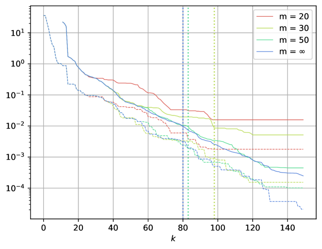
Figure 7: Relative gap (solid) and true relative gap (dashed) versus iterations for supply chain example, with finite memory values $m=20$, $m=30$, $m=50$, and $m=\infty$.

5 Conclusions

We focus on developing a good practical method for distributed convex optimization in a setting where the agents support a value/subgradient oracle, which can take substantial effort to evaluate, and the coupling among the agent variables is given explicitly and exactly as a structured convex problem, possibly including constraints. (This differs from the more typical setting, where the agent functions are differentiable and can be evaluated quickly, and the coupling function has an analytical proximal operator.) Our assumptions allow us to consider methods that carry out more computation in each iteration, such as cutting-plane or bundle methods, that typically involve the solution of a QP. We have found that a basic bundle-type method, when combined with diagonal scaling and a good algorithm parameter discovery method, gives good practical convergence across a number of problems types and sizes. Here by good practical convergence we mean that with default algorithm parameters, a reasonable approximate solution can be found in a few tens of iterations, and a higher accuracy solution (which is generally not needed in applications) can be obtained in perhaps a hundred or fewer iterations. (Theoretical convergence of the algorithm is always guaranteed.)

Our methods combines multiple variations of known techniques for bundle-type methods into a solver has a number of attractive features. First, it has essentially no algorithm parameters, and works well with the few parameters set to default values. Second, it achieves good practical convergence across a number of problems types and sizes. Third, it can warm start when the coupling changes, by saving the information obtained in previous agent evaluations.

Appendix A Convergence proof

In this section we give a proof of convergence of the bundle method for oracle-structured optimization. Our proof uses well known ideas, and borrows heavily from [Bel05]. We will make one additional (and traditional) assumption, that $f$ and $g$ are Lipschitz continuous on $\mathop{\bf dom}g$.

We say that the update was accepted in iteration $k$ if $x^{k+1}=\tilde{x}^{k+1}$. Suppose this occurs in iterations $k_{1}<k_{2}<\cdots$. We let $K=\{k_{1},k_{2},\ldots\}$ denote the set of iterations where the update was accepted. We distinguish two cases: $|K|=\infty$ and $|K|<\infty$.

Infinite updates.

We assume $|K|=\infty$. First we establish that $\delta^{k_{s}}\to 0$ as $s\to\infty$. Since $k=k_{s}$ is an accepted step, from step 6 of the algorithm we have

$$\eta\delta^{k_{s}}\leq h(x^{k_{s}})-h(x^{k_{s}+1})=h(x^{k_{s}})-h(x^{k_{s+1}}).$$

Summing this inequality from $s=1$ to $s=l$ and dividing by $\eta$ gives

$$\sum_{s=1}^{l}\delta^{k_{s}}\leq\frac{h(x^{k_{1}})-h(x^{k_{l+1}})}{\eta}\leq\frac{h(x^{0})-h^{\star}}{\eta},$$

which implies that $\delta^{k_{s}}$ is summable, and so converges to zero as $s\to\infty$.

Since $\tilde{x}^{k_{s}+1}$ minimizes $\hat{h}^{k_{s}}(x)+(\rho/2)\|x-x^{k_{s}}\|_{2}^{2}$, we have

$$\partial\hat{h}^{k_{s}}\left(\tilde{x}^{k_{s}+1}\right)+\rho(\tilde{x}^{k_{s}+1}-x^{k_{s}})\ni 0.$$

Using $\tilde{x}^{k_{s}+1}=x^{k_{s}+1}=x^{k_{s+1}}$, we have

$$\rho(x^{k_{s}}-x^{k_{s+1}})\in\partial\hat{h}^{k_{s}}\left(x^{k_{s+1}}\right).$$

It follows that

$$h^{\star}=h(x^{\star})\geq\hat{h}^{k_{s}}(x^{\star})\geq\hat{h}^{k_{s}}(x^{k_{s+1}})+\rho(x^{k_{s}}-x^{k_{s+1}})^{T}(x^{\star}-x^{k_{s+1}}).$$

We first rewrite this as

$$\frac{h^{\star}-\hat{h}^{k_{s}}(x^{k_{s+1}})}{\rho} \geq (x^{k_{s}}-x^{k_{s+1}})^{T}(x^{\star}-x^{k_{s}})+(x^{k_{s}}-x^{k_{s+1}})^{T}(x^{k_{s}}-x^{k_{s+1}}))$$

$$= (x^{k_{s}}-x^{k_{s+1}})^{T}(x^{\star}-x^{k_{s}})+\|x^{k_{s}}-x^{k_{s+1}}\|_{2}^{2},$$

and then in the form we will use below,

$$2(x^{k_{s}}-x^{k_{s+1}})^{T}(x^{\star}-x^{k_{s}})\leq(2/\rho)\left(h^{\star}-\hat{h}^{k_{s}}(x^{k_{s+1}})\right)-2\|x^{k_{s}}-x^{k_{s+1}}\|_{2}^{2}.$$

Now we use a standard subgradient algorithm argument. We have

$$\|x^{k_{s+1}}-x^{\star}\|_{2}^{2} = \|x^{k_{s}}-x^{\star}\|_{2}^{2}+\|x^{k_{s+1}}-x^{k_{s}}\|_{2}^{2}+2(x^{k_{s}}-x^{k_{s+1}})^{T}(x^{\star}-x^{k_{s}})$$

$$\leq \|x^{k_{s}}-x^{\star}\|_{2}^{2}+(2/\rho)\left(h^{\star}-\hat{h}^{k_{s}}(x^{k_{s+1}})\right)-\|x^{k_{s+1}}-x^{k_{s}}\|_{2}^{2}$$

$$= \|x^{k_{s}}-x^{\star}\|_{2}^{2}+(2/\rho)\left(h^{\star}-h(x^{k_{s}})+\delta^{k_{s}}\right).$$

Summing this inequality from $s=1$ to $s=l$ and re-arranging yields

$$(2/\rho)\sum_{s=1}^{l}\left(h(x^{k_{s}})-h^{\star}\right) \leq \|x^{k_{1}}-x^{\star}\|_{2}^{2}-\|x^{k_{l+1}}-x^{\star}\|_{2}^{2}+(2/\rho)\sum_{s=1}^{l}\delta^{k_{s}}$$

$$\leq \|x^{k_{1}}-x^{\star}\|_{2}^{2}+2(h(x^{0})-h^{\star})/\eta\rho.$$

It follows that the nonnegative series $h(x^{k_{s}})-h^{\star}$ is summable, and therefore, $h(x^{k_{s}})\to h^{\star}$ as $s\to\infty$.

Finite updates.

We assume $|K|<\infty$, with $p=\max K$ its largest entry. It follows that for any $k>p$, we have $h(x^{k})-h\left(\tilde{x}^{k+1}\right)<\eta\delta^{k}$. Note that $x^{k}=x^{p}$ for all $k\geq p+1$. Moreover, using

$$\|\tilde{x}^{k+2}-x^{p}\|_{2}^{2}=\|\tilde{x}^{k+2}-\tilde{x}^{k+1}\|_{2}^{2}+\left\|\tilde{x}^{k+1}-x^{p}\right\|_{2}^{2}-2\left(x^{p}-\tilde{x}^{k+1}\right)^{T}(\tilde{x}^{k+2}-\tilde{x}^{k+1})$$

with $\rho(x^{p}-\tilde{x}^{k+1})\in\partial\hat{h}^{k}\left(\tilde{x}^{k+1}\right)$ and $\hat{h}^{k+1}(\tilde{x}^{k+2})\geq\hat{h}^{k}(\tilde{x}^{k+2})$, we get

$$\delta^{k}-\delta^{k+1} \geq \hat{h}^{k+1}(\tilde{x}^{k+2})-\hat{h}^{k}\left(\tilde{x}^{k+1}\right)-\rho\left(x^{p}-\tilde{x}^{k+1}\right)^{T}(\tilde{x}^{k+2}-\tilde{x}^{k+1})$$

$$+(\rho/2)\left\|\tilde{x}^{k+2}-\tilde{x}^{k+1}\right\|_{2}^{2}$$

$$\geq (\rho/2)\left\|\tilde{x}^{k+2}-\tilde{x}^{k+1}\right\|_{2}^{2}.$$

Therefore, $\delta^{k}\geq\delta^{k+1}+(\rho/2)\left\|\tilde{x}^{k+2}-\tilde{x}^{k+1}\right\|_{2}^{2}$ for all $k\geq p+1$. Then from

$$\hat{h}^{k}(x^{p}) \geq \hat{h}^{k}\left(\tilde{x}^{k+1}\right)+\rho(x^{p}-\tilde{x}^{k+1})^{T}(x^{p}-\tilde{x}^{k+1})$$

$$= h(x^{k})-\delta^{k}+(\rho/2)\left\|x^{p}-\tilde{x}^{k+1}\right\|_{2}^{2},$$

it follows that $\left\|x^{p}-\tilde{x}^{k+1}\right\|_{2}^{2}\leq 2\delta^{k}/\rho\leq 2\delta^{p}/\rho$.

Now we use the assumption that $f$ and $g$ are Lipschitz continuous with Lipschitz constant $L$ for all $x\in\mathop{\bf dom}g$. Every $q\in\partial\hat{f}^{k}(x)$ has the form $q=\sum_{t\leq k}\theta_{t}q^{t}$, with $\theta_{t}\geq 0$ and $\sum_{t}\theta_{t}=1$, a convex combination of normal vectors of active constraints at $x$, where $q^{t}\in\partial f(x^{t})$. Therefore, $\hat{h}^{k}(x)=\hat{f}^{k}(x)+g(x)$ is $2L$-Lipschitz continuous.

Combining this with

$$\delta^{k}\leq h(x^{k})-\hat{h}^{k}\left(\tilde{x}^{k+1}\right),\qquad-\eta\delta^{k}\leq{h}\left(\tilde{x}^{k+1}\right)-h(x^{k}),$$

we have

$$(1-\eta)\delta^{k}\leq{h}\left(\tilde{x}^{k+1}\right)-h\left(\tilde{x}^{k}\right)+\hat{h}^{k}\left(\tilde{x}^{k}\right)-\hat{h}^{k}\left(\tilde{x}^{k+1}\right)\leq 4L\left\|\tilde{x}^{k}-\tilde{x}^{k+1}\right\|_{2}.$$

Therefore, from

$$\frac{(1-\eta)^{2}\rho}{32L^{2}}\sum_{k\geq p}\left(\delta^{k}\right)^{2}\leq\sum_{k\geq p}\left(\delta^{k}-\delta^{k+1}\right)\leq\delta^{p},$$

we can establish that $\delta^{k}$ converges to zero as $k\to\infty$. This implies

$$\underset{k\to\infty}{\lim}\left(\hat{h}^{k}\left(\tilde{x}^{k+1}\right)+(\rho/2)\left\|\tilde{x}^{k+1}-x^{p}\right\|_{2}^{2}\right)=h(x^{p}).$$

Also from $\underset{k\to\infty}{\lim}\left(h(x^{p})-h\left(\tilde{x}^{k+1}\right)\right)=0$ and $\left\|{x}^{p}-\tilde{x}^{k+1}\right\|_{2}^{2}\leq\frac{2\delta^{k}}{\rho}$, it follows that

$$\underset{k\to\infty}{\lim}\hat{h}^{k}\left(\tilde{x}^{k+1}\right)=h(x^{p}),\qquad\underset{k\to\infty}{\lim}\left\|{x}^{p}-\tilde{x}^{k+1}\right\|_{2}^{2}=0.$$

Hence, we get $0\in\partial h(x^{p})$, which implies $h(x^{p})=h^{\star}$.

References

- [AF18] W. van Ackooij and A. Frangioni. Incremental bundle methods using upper models. SIAM Journal on Optimization, 28:379–410, 2018.
- [AV95] D. S. Atkinson and P. M. Vaidya. A cutting plane algorithm for convex programming that uses analytic centers. Mathematical Programming, 69:1–43, 1995.
- [AVDB18] A. Agrawal, R. Verschueren, S. Diamond, and S. Boyd. A rewriting system for convex optimization problems. Journal of Control and Decision, 5(1):42–60, 2018.
- [BADF09] H. M. T. Ben Amor, J. Desrosiers, and A. Frangioni. On the choice of explicit stabilizing terms in column generation. Discrete Applied Mathematics, 157(6):1167–1184, 2009.
- [BDPV22] S. Boyd, J. Duchi, M. Pilanci, and L. Vandenberghe. Stanford EE 364b, lecture notes: Subgradients, 2022. URL: https://web.stanford.edu/class/ee364b/lectures/subgradients_notes.pdf. Last visited on 2022/08/04.
- [Bel05] A. Belloni. Lecture notes for IAP 2005 course introduction to bundle methods, 2005.
- [BLRS01] L. Bacaud, C. Lemaréchal, A. Renaud, and C. Sagastizábal. Bundle methods in stochastic optimal power management: A disaggregated approach using preconditioners. Computational Optimization and Applications, 20:227–244, 2001.
- [BMLRT15] R. S. Burachik, J. E. Martínez-Legaz, M. Rezaie, and M. Théra. An additive subfamily of enlargements of a maximally monotone operator. Set-Valued and Variational Analysis, 23:643–665, 2015.
- [BMR03] E. G. Birgin, J. M. Martínez, and M. Raydan. Inexact spectral projected gradient methods on convex sets. IMA Journal of Numerical Analysis, 23(4):539–559, 10 2003.
- [BPC11] S. Boyd, N. Parikh, and E. Chu. Distributed Optimization and Statistical Learning via the Alternating Direction Method of Multipliers. Now Publishers, 2011.
- [BQ00] J. V. Burke and M. Qian. On the superlinear convergence of the variable metric proximal point algorithm using Broyden and BFGS matrix secant updating. Mathematical Programming, 88:157–181, 2000.
- [Bra10] A. Bradley. Algorithms for the equilibration of matrices and their application to limited-memory Quasi-Newton methods. PhD thesis, Stanford University, CA, 2010.
- [Bru75] R. E. Bruck, Jr. An iterative solution of a variational inequality for certain monotone operators in Hilbert space. Bulletin of the American Mathematical Society, 81:890–892, 1975.
- [BV04] S. Boyd and L. Vandenberghe. Convex Optimization. Cambridge University Press, 2004.
- [CF99] X. Chen and M. Fukushima. Proximal quasi-Newton methods for nondifferentiable convex optimization. Mathematical Programming, 85(2):313–334, 1999.
- [CG59] E. W. Cheney and A. A. Goldstein. Newton’s method for convex programming and Tchebycheff approximation. Numerische Mathematik, 1:253–268, 1959.
- [CGM85] P. Concus, G. Golub, and G. Meurant. Block preconditioning for the conjugate gradient method. SIAM Journal on Scientific and Statistical Computing, 6(1):220–252, 1985.
- [CL93] R. Correa and C. Lemaréchal. Convergence of some algorithms for convex minimization. Mathematical Programming, 62:261–275, 1993.
- [CL16] Y. Choi and Y. Lim. Optimization approach for resource allocation on cloud computing for IoT. International Journal of Distributed Sensor Networks, 12(3):3479247, 2016.
- [CP11] P. L. Combettes and J.-C. Pesquet. Proximal splitting methods in signal processing. In Fixed-Point Algorithms for Inverse Problems in Science and Engineering, pages 185–212. Springer, 2011.
- [CR97] G. H. Chen and R. T. Rockafellar. Convergence rates in forward–backward splitting. SIAM Journal on Optimization, 7(2):421–444, 1997.
- [DB16] S. Diamond and S. Boyd. CVXPY: A Python-embedded modeling language for convex optimization. Journal of Machine Learning Research, 17(83):1–5, 2016.
- [DG21] M. Díaz and B. Grimmer. Optimal convergence rates for the proximal bundle method, 2021.
- [DHS11] J. Duchi, E. Hazan, and Y. Singer. Adaptive subgradient methods for online learning and stochastic optimization. Journal of Machine Learning Research, 12(7):2121–2159, 2011.
- [DV85] V. F. Dem’yanov and L. V. Vasil’ev. Nondifferentiable Optimization. Translations Series in Mathematics and Engineering. Springer New York, 1985.
- [Dí21] M. Díaz. proximal-bundle-method. https://github.com/mateodd25/proximal-bundle-method, 2021.
- [EM75] J. Elzinga and T. G. Moore. A central cutting plane algorithm for the convex programming problem. Mathematical Programming, 8:134–145, 1975.
- [ES10] G. Emiel and C. Sagastizábal. Incremental-like bundle methods with application to energy planning. Computational Optimization and Applications, 46(2):305–332, 2010.
- [FG14a] A. Frangioni and E. Gorgone. Bundle methods for sum-functions with “easy” components: Applications to multicommodity network design. Mathematical Programming, 145:133–161, 2014.
- [FG14b] A. Frangioni and E. Gorgone. Generalized bundle methods for sum-functions with “easy” components: Applications to multicommodity network design. Mathematical Programming, 145:133–161, 2014.
- [FGG04] A. Fuduli, M. Gaudioso, and G. Giallombardo. Minimizing nonconvex nonsmooth functions via cutting planes and proximity control. SIAM Journal on Optimization, 14(3):743–756, 2004.
- [Fis22] F. Fischer. An asynchronous proximal bundle method. Optimization Online, 2022.
- [Fra02] A. Frangioni. Generalized bundle methods. SIAM Journal on Optimization, 13(1):117–156, 2002.
- [Fra20] A. Frangioni. Standard bundle methods: Untrusted models and duality. In Numerical Nonsmooth Optimization, pages 61–116. Springer, 2020.
- [GBY06] M. Grant, S. Boyd, and Y. Ye. Disciplined convex programming. In Global Optimization, pages 155–210. Springer, 2006.
- [GP79] C. Gonzaga and E. Polak. On constraint dropping schemes and optimality functions for a class of outer approximations algorithms. SIAM Journal on Control and Optimization, 17(4):477–493, 1979.
- [Hin01] M. Hintermüller. A proximal bundle method based on approximate subgradients. Computational Optimization and Applications, 20(3):245–266, 2001.
- [HL08] Z. Han and K. J. R. Liu. Resource Allocation for Wireless Networks: Basics, Techniques, and Applications. Cambridge University Press, 2008.
- [HMM04] M. Haarala, K. Miettinen, and M. M. Mäkelä. New limited memory bundle method for large-scale nonsmooth optimization. Optimization Methods and Software, 19(6):673–692, 2004.
- [HMM07] N. Haarala, K. Miettinen, and M. M. Mäkelä. Globally convergent limited memory bundle method for large-scale nonsmooth optimization. Mathematical Programming, 109:181–205, 2007.
- [HP17] C. Helmberg and A. Pichler. Dynamic Scaling and Submodel Selection in Bundle Methods for Convex Optimization. Technische Universität Chemnitz, Fakultät für Mathematik, 2017.
- [HR00] C. Helmberg and F. Rendl. A spectral bundle method for semidefinite programming. SIAM Journal on Optimization, 10(3):673–696, 2000.
- [HS+52] M. Hestenes, E. Stiefel, et al. Methods of conjugate gradients for solving linear systems. Journal of Research of the National Bureau of Standards, 49(6):409–436, 1952.
- [HSS16] W. Hare, C. Sagastizábal, and M. Solodov. A proximal bundle method for nonsmooth nonconvex functions with inexact information. Computational Optimization and Applications, 63(1):1–28, 2016.
- [HUL96] J.-B. Hiriart-Urruty and C. Lemaréchal. Convex Analysis and Minimization Algorithms II: Advanced Theory and Bundle Methods. Grundlehren der mathematischen Wissenschaften. Springer Berlin Heidelberg, 1996.
- [HUL13] J.-B. Hiriart-Urruty and C. Lemaréchal. Convex Analysis and Minimization Algorithms I: Fundamentals, volume 305. Springer Science & Business Media, 2013.
- [IMdO20] F. Iutzeler, J. Malick, and W. de Oliveira. Asynchronous level bundle methods. Mathematical Programming, 184:319–348, 2020.
- [Jac45] C. Jacobi. Ueber eine neue auflösungsart der bei der methode der kleinsten quadrate vorkommenden lineären gleichungen. Astronomische Nachrichten, 22(20):297–306, 1845.
- [Kar07] N. Karmitsa. LMBM–FORTRAN subroutines for large-scale nonsmooth minimization: User’s manual’. TUCS Techn. Rep., 77:856, 2007.
- [Kar16] N. Karmitsa. Proximal bundle method. http://napsu.karmitsa.fi/proxbundle/, 2016.
- [Kel60] J. E. Kelley, Jr. The cutting-plane method for solving convex programs. Journal of the Society for Industrial and Applied Mathematics, 8(4):703–712, 1960.
- [Kiw83] K. Kiwiel. An aggregate subgradient method for nonsmooth convex minimization. Mathematical Programming, 27:320–341, 1983.
- [Kiw85] K. C. Kiwiel. An algorithm for nonsmooth convex minimization with errors. Mathematics of Computation, 45(171):173–180, 1985.
- [Kiw90] K. Kiwiel. Proximity control in bundle methods for convex nondifferentiable minimization. Mathematical Programming, 46(1-3):105–122, 1990.
- [Kiw95] K. C. Kiwiel. Approximations in proximal bundle methods and decomposition of convex programs. Journal of Optimization Theory and applications, 84(3):529–548, 1995.
- [Kiw96] K. C. Kiwiel. Restricted step and Levenberg–Marquardt techniques in proximal bundle methods for nonconvex nondifferentiable optimization. SIAM Journal on Optimization, 6(1):227–249, 1996.
- [Kiw99] K. C. Kiwiel. A bundle Bregman proximal method for convex nondifferentiable minimization. Mathematical Programming, 85(2):241–258, 1999.
- [Kiw00] K. C. Kiwiel. Efficiency of proximal bundle methods. Journal of Optimization Theory and Applications, 104(3):589–603, 2000.
- [Kiw06] K. C. Kiwiel. A proximal bundle method with approximate subgradient linearizations. SIAM Journal on Optimization, 16(4):1007–1023, 2006.
- [KM10] N. Karmitsa and M. Mäkelä. Limited memory bundle method for large bound constrained nonsmooth optimization: Convergence analysis. Optimization Methods & Software, 25(6):895–916, 2010.
- [KMA+21] P. Kairouz, H. B. McMahan, B. Avent, A. Bellet, M. Bennis, A. N. Bhagoji, K. Bonawitz, Z. Charles, G. Cormode, R. Cummings, et al. Advances and open problems in federated learning. Foundations and Trends® in Machine Learning, 14(1–2):1–210, 2021.
- [KPZ19] K. Kim, C. Petra, and V. Zavala. An asynchronous bundle-trust-region method for dual decomposition of stochastic mixed-integer programming. SIAM Journal on Optimization, 29(1):318–342, 2019.
- [KZNS21] K. Kim, W. Zhang, H. Nakao, and M. Schanen. BundleMethod.jl: Implementation of Bundle Methods in Julia, March 2021.
- [Lem75] C. Lemaréchal. An extension of Davidon methods to non differentiable problems. Mathematical Programming Study, 3:95–109, 1975.
- [Lem78] C. Lemarechal. Nonsmooth optimization and descent methods. 1978.
- [Lem01] C. Lemaréchal. Lagrangian relaxation. In Computational Combinatorial Optimization, pages 112–156. Springer, 2001.
- [LM79] P. L. Lions and B. Mercier. Splitting algorithms for the sum of two nonlinear operators. SIAM Journal on Numerical Analysis, 16(6):964–979, 1979.
- [LNN95] C. Lemaréchal, A. Nemirovskii, and Y. Nesterov. New variants of bundle methods. Mathematical Programming, 69(1):111–147, 1995.
- [LOP09] C. Lemaréchal, A. Ouorou, and G. Petrou. A bundle-type algorithm for routing in telecommunication data networks. Computational Optimization and Applications, 44:385–409, 2009.
- [LPM18] J. Lv, L. Pang, and F. Meng. A proximal bundle method for constrained nonsmooth nonconvex optimization with inexact information. Journal of Global Optimization, 70(3):517–549, 2018.
- [LS94] C. Lemaréchal and C. Sagastizábal. An approach to variable metric bundle methods. In System Modelling and Optimization, pages 144–162. Springer, 1994.
- [LS97] C. Lemaréchal and C. Sagastizábal. Variable metric bundle methods: From conceptual to implementable forms. Mathematical Programming, 76:393–410, 1997.
- [LSPR96] C. Lemaréchal, C. Sagastizábal, F. Pellegrino, and A. Renaud. Bundle methods applied to the unit-commitment problem. In System Modelling and Optimization: Proceedings of the Seventeenth IFIP TC7 Conference on System Modelling and Optimization, 1995, pages 395–402. Springer, 1996.
- [LSTS20] T. Li, A. K. Sahu, A. Talwalkar, and V. Smith. Federated learning: Challenges, methods, and future directions. IEEE Signal Processing Magazine, 37(3):50–60, 2020.
- [LV98] L. Lukšan and J. Vlček. A bundle-Newton method for nonsmooth unconstrained minimization. Mathematical Programming, 83:373–391, 1998.
- [LV99] L. Lukšan and J. Vlček. Globally convergent variable metric method for convex nonsmooth unconstrained minimization. Journal of Optimization Theory and Applications, 102:593–613, 1999.
- [LZDL05] Y. Liu, S. Zhao, X. Du, and S. Li. Optimization of resource allocation in construction using genetic algorithms. In 2005 International Conference on Machine Learning and Cybernetics, volume 6, pages 3428–3432. IEEE, 2005.
- [Mäk03] M. Mäkelä. Multiobjective proximal bundle method for nonconvex nonsmooth optimization: Fortran subroutine MPBNGC 2.0. Reports of the Department of Mathematical Information Technology, Series B. Scientific Computing, B, 13:2003, 2003.
- [MHB75] R. Marsten, W. Hogan, and J. Blankenship. The boxstep method for large-scale optimization. Operations Research, 23(3):389–405, 1975.
- [Mif77] R. Mifflin. Semismooth and semiconvex functions in constrained optimization. SIAM Journal on Control and Optimization, 15(6):959–972, 1977.
- [Mif96] R. Mifflin. A quasi-second-order proximal bundle algorithm. Mathematical Programming, 73(1):51–72, 1996.
- [MKW16] M. Mäkelä, N. Karmitsa, and O. Wilppu. Proximal bundle method for nonsmooth and nonconvex multiobjective optimization. Mathematical Modeling and Optimization of Complex Structures, pages 191–204, 2016.
- [Nes83] Y. Nesterov. A method for solving the convex programming problem with convergence rate . Proceedings of the USSR Academy of Sciences, 269:543–547, 1983.
- [NW99] J. Nocedal and S. Wright. Numerical Optimization. Springer, 1999.
- [OE15] W. de Oliveira and J. Eckstein. A bundle method for exploiting additive structure in difficult optimization problems. Optimization Online, 2015.
- [OMV00] A. Ouorou, P. Mahey, and J.-Ph. Vial. A survey of algorithms for convex multicommodity flow problems. Management Science, 46(1):126–147, 2000.
- [OS16] W. de Oliveira and M. Solodov. A doubly stabilized bundle method for nonsmooth convex optimization. Mathematical Programming, 156(1):125–159, 2016.
- [OS20] W. de Oliveira and M. Solodov. Bundle methods for inexact data. In Numerical Nonsmooth Optimization, pages 417–459. Springer, 2020.
- [OSL14] W. de Oliveira, C. Sagastizábal, and C. Lemaréchal. Convex proximal bundle methods in depth: a unified analysis for inexact oracles. Mathematical Programming, 148:241–277, 2014.
- [Pas79] G. B. Passty. Ergodic convergence to a zero of the sum of monotone operators in Hilbert space. Journal of Mathematical Analysis and Applications, 72(2):383–390, 1979.
- [PB+14] N. Parikh, S. Boyd, et al. Proximal algorithms. Foundations and Trends® in Optimization, 1(3):127–239, 2014.
- [Roc81] R. T. Rockafellar. The Theory of Subgradients and its Applications to Problems of Optimization. Heldermann Verlag, 1981.
- [RS02a] P. Rey and C. Sagastizábal. Dynamical adjustment of the prox-parameter in bundle methods. Optimization, 51(2):423–447, 2002.
- [RS02b] P. A. Rey and C. Sagastizábal. Dynamical adjustment of the prox-parameter in bundle methods. Optimization, 51(2):423–447, 2002.
- [Sch22] S. Schechtman. Stochastic proximal subgradient descent oscillates in the vicinity of its accumulation set. Optimization Letters, pages 1–14, 2022.
- [Sho12] N. Z. Shor. Minimization Methods for Non-differentiable Functions, volume 3. Springer Science & Business Media, 2012.
- [Sin64] R. Sinkhorn. A relationship between arbitrary positive matrices and doubly stochastic matrices. The Annals of Mathematical Statistics, 35(2):876–879, 1964.
- [SNW12] Suvrit Sra, S. Nowozin, and S. J. Wright. Optimization for Machine Learning. Mit Press, 2012.
- [SZ92] H. Schramm and J. Zowe. A version of the bundle idea for minimizing a nonsmooth function: Conceptual idea, convergence analysis, numerical results. SIAM Journal on Optimization, 2(1):121–152, 1992.
- [TJ16] R. Takapoui and H. Javadi. Preconditioning via diagonal scaling. 2016.
- [TMAS16] T. Trisna, M. Marimin, Y. Arkeman, and T. Sunarti. Multi-objective optimization for supply chain management problem: A literature review. Decision Science Letters, 5(2):283–316, 2016.
- [TVSL10] C. H. Teo, S.V.N. Vishwanathan, A. Smola, and Q. Le. Bundle methods for regularized risk minimization. Journal of Machine Learning Research, 11(1), 2010.
- [vABdOS17] W. van Ackooij, V. Berge, W. de Oliveira, and C. Sagastizábal. Probabilistic optimization via approximate -efficient points and bundle methods. Computers & Operations Research, 77:177–193, 2017.
- [vAFdO16] W. van Ackooij, A. Frangioni, and W. de Oliveira. Inexact stabilized Benders’ decomposition approaches with application to chance-constrained problems with finite support. Computational Optimization and Applications, 65:637–669, 2016.
- [WP95] T. Westerlund and F. Pettersson. An extended cutting plane method for solving convex MINLP problems. Computers Chemical Engineering, 19:131–136, 1995.
- [WZX+20] F. Wei, X. Zhang, J. Xu, J. Bing, and G. Pan. Simulation of water resource allocation for sustainable urban development: An integrated optimization approach. Journal of Cleaner Production, 273:122537, 2020.
- [YW06] P. Yin and J. Wang. Ant colony optimization for the nonlinear resource allocation problem. Applied Mathematics and Computation, 174(2):1438–1453, 2006.
- [ZBL+21] B. Zhou, J. Bao, J. Li, Y. Lu, T. Liu, and Q. Zhang. A novel knowledge graph-based optimization approach for resource allocation in discrete manufacturing workshops. Robotics and Computer-Integrated Manufacturing, 71:102160, 2021.