Asymptotic preserving schemes for nonlinear kinetic equations leading to volume-exclusion chemotaxis in the diffusive limit

Abstract

In this work we first prove, by formal arguments, that the diffusion limit of nonlinear kinetic equations, where both the transport term and the turning operator are density-dependent, leads to volume-exclusion chemotactic equations. We generalise an asymptotic preserving scheme for such nonlinear kinetic equations based on a micro-macro decomposition. By properly discretizing the nonlinear term implicitly-explicitly in an upwind manner, the scheme produces accurate approximations also in the case of strong chemosensitivity. We show, via detailed calculations, that the scheme presents the following properties: asymptotic preserving, positivity preserving and energy dissipation, which are essential for practical applications. We extend this scheme to two dimensional kinetic models and we validate its efficiency by means of 1D and 2D numerical experiments of pattern formation in biological systems.

1 Introduction

Chemotaxis is the mechanism by which cells and organisms adapt their movement in response to a chemical stimulus present in their environment. This phenomenon has been observed in many biological systems [2, 18, 17, 28].

The mathematical study of chemotaxis started from the seminal contributions of Patlak [27] and Keller and Segel [19, 20], where the authors introduced the celebrated Patlak-Keller-Segel (PKS) model. This model was originally proposed for pattern formation in bacterial populations through an advection-diffusion system of two coupled parabolic equations describing the evolution of the cell density and the chemoattractant (see [13] for a review about Keller-Segel type models). The PKS original model has been modified by various authors, with the aim of improving its consistency with biological systems. One example is the volume-exclusion chemotactic system introduced by Hillen and Painter [26] to take into account the finite size of the cells and volume limitations. In such models the chemotactic sensitivity (i.e. the term leading to cell aggregation) depends on both the chemical concentration in the medium and the local cell density, thus, the population density directly modulates its own sensitivity response. The coupled system reads, in it’s parabolic-elliptic form as

$$\partial_{t}\rho-\nabla\cdot\left(D_{\rho}(q(\rho)-\rho q^{\prime}(\rho))\nabla\rho-\chi_{0}q(\rho)\rho\nabla c\right) =h(\rho,c)\ ,\ \qquad t\geq 0\ ,\mathbf{x}\in\Omega\subset\mathbb{R}^{n}\ ,$$ (1)

$$D_{c}\Delta c+g(\rho,c) =0\ .$$

Here, $\rho(t,\mathbf{x})$ is the cell density, $c(t,\mathbf{x})$ is the chemoattractant concentration and $q(\rho)$ is a function that describes the packing capacity of the cell aggregates. The diffusion coefficients for the cells and chemoattractant are $D_{\rho}$ and $D_{c}$, respectively, and $\chi_{0}$ is the chemotactic sensitivity. The proliferation (or death) of the cells is described by $h(\rho,c)$ and the production and consumption of the chemoattractant is given by $g(\rho,c)$. Note that the classical PKS model is recovered by taking $q(\rho)=1$ in (1). It has been shown [34, 5, 35] that such volume-exclusion effect prevents blow-ups in finite time compared to the model without density effects (with $q(\rho)=1$). The volume-exclusion chemotactic equations have been widely studied in the literature, from a modelling [26, 32], analytic [34, 12, 22, 9] and numerical perspectives [14], and they have proven to be successful at describing aggregation phenomena [1, 4].

A natural question that arises is whether the volume-exclusion Keller-Segel equation (1) proposed in [26] could be obtained as the diffusion limit of a kinetic ‘velocity jump’ model [23], giving insights into how the individual mechanisms at the cell level can lead to volume-exclusion effects at the population level. In this paper, inspired by the approach followed in [25, 24], we show, by formal arguments, that the system (1) can be obtained in the diffusion limit of a nonlinear kinetic equation, provided that both the transport term and the turning operator are density-dependent (Theorem 1 in Section 2.2). The corresponding kinetic ‘velocity jump’ model we propose reads

$$\partial_{t}f+\mathbf{v}\cdot\nabla(F[\rho](t,\mathbf{x},\mathbf{v})f)=\lambda q(\rho)(-f+\rho T(\mathbf{v},\rho,\nabla c))\ ,$$ (2)

where $f(t,\mathbf{x},\mathbf{v})\geq 0$ is the phase space cell density, $\mathbf{x}\in\Omega\subset\mathbb{R}^{n}$ denotes the position, $\mathbf{v}\in V\subset\mathbb{R}^{n}$ is the velocity where $V$ denotes the unit sphere $V=\{\mathbf{x}\in\mathbb{R}^{n}:\ |\mathbf{x}|=1\}$, and $t\in\mathbb{R}^{+}$ the time. Here, $\lambda$ is the constant turning rate, with $1/\lambda$ giving a measure of the mean run length between velocity jumps, $T(\mathbf{v},\rho,\nabla c)$ gives the probability of a velocity jump to velocity $\mathbf{v}$, which depends on the chemical concentration $c$ and the term $F[\rho](t,\mathbf{x},\mathbf{v})$ describes the anisotropic transport due to the density limited motion.

We then numerically investigate whether the relevant macroscopic volume-exclusion equation corresponds to the underlying physical system described by the kinetic equation in the diffusion limit. These methods are widely known as asymptotic preserving schemes (AP) [11, 15] since they mimic the asymptotic behaviour of the kinetic equation when the scaling parameter approaches to zero and the mesh size and time steps are fixed. In this paper, we use a micro-macro decomposition of the unknown in the sense of [21] as detailed in Section 3. The finite difference discretization is explained in Section 4, where a proper implicit-explicit discretization of the nonlinear terms including the chemosensitivity term is applied to improve the efficiency and stability of our numerical scheme. This decomposition of the solution of the kinetic equation is analogous to a Chapman-Enskog expansion in the case of the classical Boltzmann equation. It uses the properties of the “collisional operator”, which in our formulation describes the run and tumble movement of the individual. For the kinetic counterpart of the classical PKS equations we refer to [7], where the authors used an odd-even splitting at the kinetic level and studied the behaviour of solutions (blow up). Other related works can be found in [10, 31, 16].

The volume-exclusion PKS for modelling tumor growth

In real-world applications, mathematical models provide useful tools towards identifying links between phenomena observed at the macroscopic level and the underlying microscopic properties. Chemotactic models have been extensively used to describe glioblastoma (GBM) aggregates [30] and in particular, the volume-exclusion system (1) was used in [1] to explain the mechanical changes at the cell level in these systems due to the presence of a chemical treatment. In this work, the cell’s elasticity is modelled through the term $q(\rho)$ which incorporates the cell-cell interactions [33]. This function $q(\rho)$ can be explicitly written as $q(\rho)=1-(\rho/\bar{\rho})^{\gamma}$ where $\gamma$ is a parameter that depends on the concentration of the treatment and $\bar{\rho}$ is the maximum cell density in each aggregate. For $\gamma=1$ the cells are considered as solid particles while $\gamma>1$ corresponds to semi-elastic particles that can squeeze into empty spaces.

A drawback of this approach is that it is formulated directly at the continuous (PDE) level, therefore the interactions comprised in such models are mostly based on phenomenological considerations at the population level. However, neglecting the microstructural features causes these models to fail to predict the micromechanical behaviors, which makes the validation of these approaches difficult due to the lack of physical mechanisms to interpret the population macroscopic behavior. Establishing the link between macroscopic models and their microscopic counterparts, the central task of kinetic theory, can benefit macroscopic models gain in predictive character and become invaluable aids for experimental data analysis. This paper aims to take a step in this direction, by providing an interpretation of the volume-filling chemotactic system as the diffusion limit of a kinetic ’velocity jump’ model which gives a more direct interpretation of the PDE operators in terms of more fundamental characteristics of the motion. We then validate this limit using an AP numerical scheme.

Outline of the paper

This paper is organized as follows. In Section 2 we introduce the new version of the kinetic ‘velocity jump’ model given by (2) and consider its diffusion limit using a Hilbert expansion method as in [25] under appropriate scaling assumptions for the turning operator. We show that the limiting system has a dissipating free energy and derive an energy estimate used to validate the numerical method. In Section 3, we present the micro-macro decomposition of a slightly modified version of the kinetic model taking into account a proliferation term. Section 4 is devoted to the design of an AP scheme and the study of its properties (positivity preserving, AP etc). Finally, we present the numerical experiments and draw conclusions in Section 5.

2 Volume-exclusion kinetic equation: Macroscopic limit

In this section we analyse the diffusion limit of the following transport equation

$$\partial_{t}f+\mathbf{v}\cdot\nabla(F[\rho](t,\mathbf{x},\mathbf{v})f)=\lambda q(\rho)(-f+\rho T(\mathbf{v},\rho,\nabla c))\ .$$

The turning kernel is supposed to be independent on the previous velocity of the jumping particle, and only dependent on the new velocity $\mathbf{v}$, the chemical concentration $c(t,\mathbf{x})$ and the density of particles $\rho(t,\mathbf{x})=\int_{V}f(t,\textbf{x},\mathbf{v})\mathop{}\!\mathrm{d}\mathbf{v}$ near position $\mathbf{x}$. The function $q(\rho)$ is the probability for a cell to find space at its neighbouring locations, and we assume that only a finite number of cells, $\bar{\rho}$, can be accommodated at any site. We will therefore consider functions $q(\rho)$ such that

$$q(\bar{\rho})=0\quad\text{and}\quad q(\rho)\geq 0\quad\text{for all }\;0\leq\rho\leq\bar{\rho}\ .$$

We suppose that the turning kernel $T$ integrates to 1 in the velocity variable,

$$\int_{V}T(\textbf{v},\rho,\nabla c)\mathop{}\!\mathrm{d}\mathbf{v}=1\ .$$

In the volume-exclusion approach, following the lines of [13], we assume that the probability of making a jump depends upon the availability of space into which it can move. To this aim, we suppose that cells can only make a turn in directions where space is available, and we choose the turning operator $T$ to be

$$T(\mathbf{v},\rho,\nabla c)=\tilde{c}(t,\mathbf{x})\psi(\mathbf{v},\nabla c)q(\rho(t,\mathbf{x}+\mathbf{v}))\ ,$$

where $\tilde{c}(t,\mathbf{x})$ is a normalisation factor given by

$$\tilde{c}(t,\mathbf{x})=\frac{1}{\displaystyle\int_{V}\psi(\mathbf{v},\nabla c)q(\rho(t,\mathbf{x}+\mathbf{v}))\mathop{}\!\mathrm{d}\mathbf{v}}\ .$$

Note that under these assumptions, particles will only make a turn (i) if they are not already trapped in a high density region (where they stop) and (ii) only in directions where the density of cells is not already too large.

In order to take into account density limited motion, we will also consider that cells are only transported to non-overcrowded regions, and choose for the transport term

$$F[\rho](t,\mathbf{x},\mathbf{v})=q\big{(}\rho(t,\mathbf{x}+\mathbf{v})\big{)}\ .$$

2.1 Diffusion scaling

Following the lines of [13], we aim to obtain a macroscopic limit by choosing space and time scales on which there are many velocity jumps in one order of time, but small net displacements on this time scale. To this aim, we define the dimensionless velocity, space and time variables as

$$\mathbf{u}=\frac{\mathbf{v}}{s}\ ,\quad\mathbf{\xi}=\frac{\mathbf{x}}{L}\ ,\quad\tau=\frac{t}{\sigma}\ ,$$

where $s$ is the characteristic speed, $L$ the characteristic length scale and $\sigma$ yet to be determined. Equation (2) now writes,

$$\frac{1}{\tau}\partial_{\tau}\tilde{f}+\frac{s}{L}\mathbf{u}\cdot\nabla_{\xi}(F[\tilde{\rho}](\tau,\mathbf{\xi},\mathbf{u})\tilde{f})=\lambda q(\tilde{\rho})(-\tilde{f}+\tilde{\rho}T(\mathbf{u},\tilde{\rho},\nabla c))\ ,$$ (3)

where $\tilde{f}(\mathbf{\xi},\mathbf{u},\tau)=f(\sigma\tau,L\mathbf{\xi},s\mathbf{u},t)$, $\tilde{\rho}(\tau,\mathbf{\xi})=\rho(\sigma t,L\mathbf{\xi})$ and therefore

$$F[\tilde{\rho}](\tau,\mathbf{\xi},\mathbf{u})=q(\tilde{\rho}(\tau,\mathbf{\xi}+\frac{s}{L}\mathbf{u})\ .$$

We estimate the diffusion coefficient as the product of the characteristic speed times the distance traveled between velocity jumps, giving $D\approx\mathcal{O}(\frac{s^{2}}{\lambda})$, and we deduce the characteristic diffusion time on the length scale $L$ by $\tau_{diff}\approx\frac{L^{2}\lambda}{s^{2}}$. The characteristic drift time is defined by $\tau_{drift}=\frac{L}{s}$ and we assume that the space scale is such that $\tau_{run}=\frac{1}{\lambda}\ll\tau_{drift}\ll\tau_{diff}$. We therefore introduce a small parameter $\varepsilon\ll 1$ and ensure that $\tau_{run}=\mathcal{O}(1)$, $\tau_{drift}=\mathcal{O}(\frac{1}{\varepsilon})$ and $\tau_{diff}=\mathcal{O}(\frac{1}{\varepsilon^{2}})$ by choosing the time and space scales to be $L\approx\mathcal{O}(\frac{s}{\varepsilon})$ and $\sigma=\tau_{diff}$. Without loss of generality, we set $\lambda=1$ and now equation (3) becomes (dropping the tildes and, with a slight abuse of notations, going back to $\mathbf{x},\mathbf{v}$ and $t$ for the dimensionless quantities $\xi,\mathbf{u}$ and $\tau$),

$$\varepsilon^{2}\partial_{t}f^{\varepsilon}+\varepsilon\mathbf{v}\cdot\nabla(F_{\varepsilon}[\rho](t,\mathbf{x},\mathbf{v})f^{\varepsilon})=q(\rho)(-f^{\varepsilon}+\rho T_{\varepsilon}(\mathbf{v},\rho,\nabla c))\ ,$$ (4)

where

$$T_{\varepsilon}(\mathbf{v},\rho,\nabla c)=\frac{\psi_{\varepsilon}(\mathbf{v},\nabla c)q(\rho(t,\mathbf{x}+\varepsilon\mathbf{v}))}{\displaystyle\int_{V}\psi_{\varepsilon}(\mathbf{v},\nabla c)q(\rho(t,\mathbf{x}+\varepsilon\mathbf{v}))\mathop{}\!\mathrm{d}\mathbf{v}}\ ,\qquad F_{\varepsilon}[\rho](t,\mathbf{x},\mathbf{v})=q(\rho(t,\mathbf{x}+\varepsilon\mathbf{v}))\ .$$ (5)

We will consider that the dependency of the turning operator on the chemical gradient $\nabla c$ happens as a perturbation of magnitude $\varepsilon$ in the following way

$$\psi_{\varepsilon}(\mathbf{v},\nabla c)=\psi_{0}(\mathbf{v})+\varepsilon\psi_{1}(\mathbf{v},\nabla c)\ .$$ (6)

Moreover, we will consider that $\langle\psi_{\varepsilon}\rangle=\int_{V}\psi_{\varepsilon}(\mathbf{v},\nabla c)\mathop{}\!\mathrm{d}\mathbf{v}=1$, where $\psi_{\varepsilon}(\mathbf{v},\nabla c)$ is non-negative and decreasing in $\nabla c$, which means that cells are less likely to tumble when the chemical gradient increases. In order to recover the volume-exclusion Keller-Segel equation, we will assume that $\psi_{0}$ is radially symmetric and that the perturbation $\psi_{1}(\mathbf{v},\nabla c)$ depends linearly on the chemical gradient $\nabla c$. These assumptions lead to the following hypotheses:

Hypothesis 1

$$\int_{V}\psi_{0}(\mathbf{v})\mathop{}\!\mathrm{d}\mathbf{v}=1\ ,\quad\int_{V}\psi_{1}(\mathbf{v},\nabla c)\mathop{}\!\mathrm{d}\mathbf{v}=0\ ,$$ (H1)

Hypothesis 2

$$\int_{V}\mathbf{v}\psi_{0}(\mathbf{v})\mathop{}\!\mathrm{d}\mathbf{v}=0\ ,\quad\psi_{1}(\mathbf{v},\nabla c)=\phi(\mathbf{v})\cdot\nabla c\ .$$ (H2)

2.2 Macroscopic model

In this section we prove the following theorem:

Theorem 1.

(formal) The limit $\varepsilon\rightarrow 0$ of $f^{\varepsilon}$ solving (4)-(6) together with Hypotheses H1 and H2 is $f^{0}=\rho(t,\mathbf{x})\psi_{0}(\mathbf{v})$, where $\rho$ solves

$$\partial_{t}\rho-\nabla\cdot\left(D_{0}\big{(}q(\rho)-\rho q^{\prime}(\rho)\big{)}\nabla\rho-\beta\rho q(\rho)\nabla c\right)=0\ ,$$ (7)

with the diffusion coefficient $D_{0}$ and the chemotactic sensitivity parameter $\beta$ given by

$$D_{0}=\langle(\mathbf{v}\otimes\mathbf{v})\psi_{0}(\mathbf{v})\rangle\qquad\textnormal{and}\qquad\beta=\langle\mathbf{v}\otimes\phi(\mathbf{v})\rangle\ .$$ (8)

Proof.

We first expand the transport quantity $F_{\varepsilon}$ and the turning operator $T_{\varepsilon}$ given by (5). For $\varepsilon\ll 1$, we have

$$F_{\varepsilon}[\rho]=q(\rho(t,\mathbf{x}+\varepsilon\mathbf{v}))=q(\rho(t,\mathbf{x}))+\varepsilon q^{\prime}(\rho(t,\mathbf{x}))\mathbf{v}\cdot\nabla\rho(t,\mathbf{x})+\mathcal{O}(\varepsilon^{2})\ ,$$ (9)

where $q^{\prime}(\rho)=\frac{\mathop{}\!\mathrm{d}q}{\mathop{}\!\mathrm{d}\rho}$. Introducing this expansion in the expression for $T_{\varepsilon}$, we write

$$\tilde{c}(t,\mathbf{x})=\frac{1}{q(\rho)\langle\psi_{\varepsilon}\rangle}\Bigl{(}1-\varepsilon\frac{q^{\prime}(\rho)}{q(\rho)}\nabla\rho\cdot\frac{\langle\mathbf{v}\psi_{\varepsilon}\rangle}{\langle\psi_{\varepsilon}\rangle}\Bigr{)}\ ,$$

where $\langle\psi_{\varepsilon}\rangle=\int_{V}\psi_{\varepsilon}(\mathbf{v},\nabla c)\mathop{}\!\mathrm{d}\mathbf{v}$ and $\langle\mathbf{v}\psi_{\varepsilon}\rangle=\int_{V}\mathbf{v}\psi_{\varepsilon}(\mathbf{v},\nabla c)\mathop{}\!\mathrm{d}\mathbf{v}$ denote the first and second moments of $\psi_{\varepsilon}$. Finally, we obtain

$$T_{\varepsilon}(\mathbf{v},\rho,\nabla c)=\frac{\psi_{\varepsilon}(\mathbf{v},\nabla c)}{\langle\psi_{\varepsilon}\rangle}+\varepsilon\frac{q^{\prime}(\rho)}{q(\rho)}\frac{\psi_{\varepsilon}(\mathbf{v},\nabla c)}{\langle\psi_{\varepsilon}\rangle}\nabla\rho\cdot\left(\mathbf{v}-\frac{\langle\mathbf{v}\psi_{\varepsilon}\rangle}{\langle\psi_{\varepsilon}\rangle}\right)+\mathcal{O}(\varepsilon^{2})\ .$$

Note that the error terms contained in $\mathcal{O}(\varepsilon^{2})$ integrate to 0 in the velocity variable. Using (6), the turning kernel $T_{\varepsilon}$ writes

$$T_{\varepsilon}(\mathbf{v},\rho,\nabla c)= \psi_{0}(\mathbf{v})+\varepsilon\Bigl{(}\psi_{1}(\mathbf{v},\nabla c)+\frac{q^{\prime}(\rho)}{q(\rho)}(\mathbf{v}\cdot\nabla\rho)\psi_{0}(\mathbf{v})\Bigr{)}+{\mathcal{O}(\varepsilon^{2})}\ ,$$ (10)

where the $\mathcal{O}(\varepsilon^{2})$-term is such that $\langle\mathcal{O}(\varepsilon^{2})\rangle=0$. We also note that using Hypotheses H1 and H2 we have $\langle T_{\varepsilon}\rangle=1$ which describes the conservation of individuals during the velocity reorientation. We now consider a second order regular expansion of $f^{\varepsilon}$ in $\varepsilon$,

$$f^{\varepsilon}(t,\mathbf{x},\mathbf{v})=f^{0}(t,\mathbf{x},\mathbf{v})+\varepsilon f^{1}(t,\mathbf{x},\mathbf{v})+\varepsilon^{2}f^{2}(t,\mathbf{x},\mathbf{v})+\mathcal{O}(\varepsilon^{3})\ ,$$

where $\int_{V}f^{\varepsilon}(t,\mathbf{x},\mathbf{v})\mathop{}\!\mathrm{d}\mathbf{v}=\int_{V}f^{0}(t,\mathbf{x},\mathbf{v})\mathop{}\!\mathrm{d}\mathbf{v}=\rho(t,\mathbf{x})$, therefore $\int_{V}f^{i}(t,\mathbf{x},\mathbf{v})\mathop{}\!\mathrm{d}\mathbf{v}=0$, $\forall i\geq 1$. Introducing this ansatz in (4), we obtain

$$\varepsilon^{2}\partial_{t} f^{0}+\varepsilon\mathbf{v}\cdot\nabla\big{(}q(\rho)\big{(}f^{0}+\varepsilon f^{1}\big{)}+\varepsilon q^{\prime}(\rho)(\mathbf{v}\cdot\nabla\rho)f^{0}\big{)}$$

$$= q(\rho)\Bigl{[}-f^{0}+\rho\psi_{0}(\mathbf{v})+\varepsilon\Bigl{(}(-f^{1}+\rho\Bigl{(}\psi_{1}(\mathbf{v},\nabla c)+\frac{q^{\prime}(\rho)}{q(\rho)}(\mathbf{v}\cdot\nabla\rho)\psi_{0}(\mathbf{v})\Bigr{)}\Bigr{)}{+\mathcal{O}(\varepsilon^{2})}\Bigr{]}\ .$$

Identifying the different equations in powers of $\varepsilon$, we obtain

$$\varepsilon^{0}: \ f^{0}(t,\mathbf{x},\mathbf{v})=\rho(t,\mathbf{x})\psi_{0}(\mathbf{v})\ ,$$ (11)

$$\varepsilon^{1}: \ \mathbf{v}\cdot\nabla(q(\rho)f^{0})=q(\rho)\left(-f^{1}+\rho\left(\psi_{1}(\mathbf{v},\nabla c)+\frac{q^{\prime}(\rho)}{q(\rho)}(\mathbf{v}\cdot\nabla\rho)\psi_{0}(\mathbf{v})\right)\right)\ ,$$ (12)

$$\varepsilon^{2}: \ \partial_{t}f^{0}+\mathbf{v}\cdot\nabla\bigg{(}q(\rho)f^{1}+q^{\prime}(\rho)(\mathbf{v}\cdot\nabla\rho)f^{0}\bigg{)}={\mathcal{O}(\varepsilon^{2})}\ .\$$ (13)

Integrating (13) with respect to $\mathbf{v}\in V$ and noticing that the right hand terms integrate to zero using Hypothesis H1, we get

$$\partial_{t}\rho+\nabla\cdot\left(q(\rho)\langle\mathbf{v}f^{1}\rangle+\rho q^{\prime}(\rho)\langle(\mathbf{v}\otimes\mathbf{v})\psi_{0}\rangle\nabla\rho\right)=0\ .$$ (14)

Next, after replacing $f^{0}$ by its expression (Eq. (11)), we multiply (12) by $\mathbf{v}$ and we integrate again with respect to $\mathbf{v}$ to obtain

$$q(\rho)\langle\mathbf{v}f^{1}\rangle =-\nabla\cdot\big{(}\rho q(\rho)\langle(\mathbf{v}\otimes\mathbf{v})\psi_{0}\rangle\big{)}+\rho q(\rho)\langle\mathbf{v}\psi_{1}\rangle+\rho q^{\prime}(\rho)\langle(\mathbf{v}\otimes\mathbf{v})\psi_{0}\rangle\nabla\rho\ .$$ (15)

Substituting (15) into (14) we get

$$\partial_{t}\rho+\nabla\cdot\Bigl{[}-\langle(\mathbf{v}\otimes\mathbf{v})\psi_{0}\rangle\nabla(\rho q(\rho)) +\rho q(\rho)\langle\mathbf{v}\psi_{1}\rangle$$

$$+2\rho q^{\prime}(\rho)\langle(\mathbf{v}\otimes\mathbf{v})\psi_{0}\rangle\nabla\rho\Bigr{]}=0\ .$$

Noting that $\nabla(q(\rho)\rho)=q^{\prime}(\rho)\rho\nabla\rho+q(\rho)\nabla\rho$ and using Hypothesis H2 for the perturbation $\psi_{1}$, we finally arrive to the volume-exclusion Keller-Segel model (7) together with (8). ∎

This macroscopic equation describes the volume-exclusion chemotactic motion associated with the so-called squeezing probability $q(\rho)$. Depending on the choice of this function we can consider the cells either as solid blocks, for the case $q(\rho)=1-\frac{\rho}{\bar{\rho}}$, where $\bar{\rho}$ is the maximum cell density in each aggregate, or as semi-elastic entities for $q(\rho)=1-\left(\frac{\rho}{\bar{\rho}}\right)^{\gamma}$ (see [33]). In Appendix A, we show that equation (7) admits an energy functional decreasing in time.

3 Micro-macro decomposition

In this section, we will consider a more general volume-exclusion kinetic model by including a proliferation term with the appropriate scaling

$$\varepsilon^{2}\partial_{t}f+\varepsilon{\mathbf{v}}\cdot\nabla(F_{\varepsilon}(\rho)f)=q(\rho)\left(-f+\rho T_{\varepsilon}({\mathbf{v}},\rho,\nabla c)\right)+\varepsilon^{2}r_{0}f\left(1-\rho/\rho_{\textnormal{max}}\right)_{+}\ ,$$

where $\rho_{\textnormal{max}}$ is the carrying capacity, and the transport quantity $F_{\varepsilon}(\rho)$ and the turning operator $T_{\varepsilon}$ are defined in (9) and (10), respectively. As we are interested in the limit of small $\varepsilon$, we will consider from now on a slightly modified version of the kinetic model by truncating $F_{\varepsilon}$ and $T_{\varepsilon}$ to the first order and solving the approximate equation

$$\varepsilon^{2}\partial_{t}f+\varepsilon{\mathbf{v}}\cdot\nabla(\tilde{F}_{\varepsilon}(\rho)f)=q(\rho)\left(-f+\rho\tilde{T}_{\varepsilon}({\mathbf{v}},\rho,\nabla c)\right)+\varepsilon^{2}r_{0}f\left(1-\rho/\rho_{\textnormal{max}}\right)_{+}\ ,$$ (16)

where

$$\tilde{F}_{\varepsilon}=q(\rho(t,{\mathbf{x}}))+\varepsilon q^{\prime}(\rho(t,{\mathbf{x}})){\mathbf{v}}\cdot\nabla\rho(t,{\mathbf{x}})\ ,$$

$$\tilde{T}_{\varepsilon}=\psi_{0}({\mathbf{v}})+\varepsilon\left(\psi_{1}({\mathbf{v}},\nabla c)+\frac{q^{\prime}(\rho)}{q(\rho)}({\mathbf{v}}\cdot\nabla\rho)\psi_{0}({\mathbf{v}})\right)\ .$$

With a similar argument as in the proof of Theorem 1, we can show that the approximate generalized kinetic model (16) converges to the following macroscopic limit as $\varepsilon\to 0$

$$\partial_{t}\rho-\nabla\cdot\left[D_{0}\left(q(\rho)-\rho q^{\prime}(\rho)\right)\nabla\rho-\langle{\mathbf{v}}\psi_{1}\rangle\rho q(\rho)\right]=r_{0}\rho\left(1-\rho/\rho_{\rm max}\right)_{+}\ ,$$ (17)

where $D_{0}=\langle({\mathbf{v}}\otimes{\mathbf{v}})\psi_{0}\rangle$ and $\langle\mathbf{v}\psi_{1}\rangle=\langle\mathbf{v}\phi(\mathbf{v})\rangle\nabla c=\beta\nabla c$.

To design an asymptotic preserving scheme which automatically preserves the macroscopic limit, a micro-macro formulation needs to be derived. We decompose the solution $f(t,{\mathbf{x}},{\mathbf{v}})$ as

$$f(t,{\mathbf{x}},{\mathbf{v}})=\rho(t,{\mathbf{x}})\psi_{0}({\mathbf{v}})+\varepsilon g(t,{\mathbf{x}},{\mathbf{v}})\ .$$ (18)

We note that $\langle g\rangle=0$ and the transport term is given by

$${\mathbf{v}}\cdot\nabla(\tilde{F}_{\varepsilon}(\rho)f) =({\mathbf{v}}\psi_{0})\cdot\nabla(\rho q(\rho))+\varepsilon{\mathbf{v}}\cdot\nabla\left[q(\rho)g+({\mathbf{v}}\cdot\nabla\rho)\rho q^{\prime}(\rho)\psi_{0}\right]$$

$$=({\mathbf{v}}\psi_{0})\cdot\nabla(\rho q(\rho))+\varepsilon{\mathbf{v}}\cdot\nabla(q(\rho)g)+\varepsilon\nabla\cdot(\rho q^{\prime}(\rho)({\mathbf{v}}\otimes{\mathbf{v}})\psi_{0}\nabla\rho)\ .$$

Substituting the micro-macro decomposition of $f(t,{\mathbf{x}},{\mathbf{v}})$ given by (18) into the generalized volume-exclusion kinetic model (16), integrating over ${\mathbf{v}}$ and noticing the fact that $\langle{\mathbf{v}}\psi_{0}\rangle=0,\,\langle T_{\varepsilon}\rangle=1\,\textnormal{and}\,\langle f\rangle=\rho$, we have the equation for the macroscopic quantity $\rho(t,{\mathbf{x}})$

$$\partial_{t}\rho+\langle{\mathbf{v}}\cdot\nabla(q(\rho)g)\rangle+\nabla\cdot(q^{\prime}(\rho)\rho D_{0}\nabla\rho)=r_{0}\rho\left(1-\rho/\rho_{\rm max}\right)_{+}\ .$$

To get the equation for $g$, we use the projection technique. For simplicity of notations, we introduce the projection operator $\Pi$ defined as

$$\Pi f(t,\mathbf{v},\mathbf{x})=\langle f(t,\mathbf{v},\mathbf{x})\rangle\psi_{0}(\mathbf{v})\ .$$

It is easy to check that, for $I$ the identity operator,

$$(I-\Pi)f=\varepsilon(I-\Pi)g=\varepsilon g\ ,$$

$$(I-\Pi)({\mathbf{v}}\cdot\nabla(\tilde{F}_{\varepsilon}f))=({\mathbf{v}}\psi_{0})\cdot\nabla(q(\rho)\rho)+\varepsilon(I-\Pi)\left[{\mathbf{v}}\cdot\nabla(q(\rho)g)+\nabla\cdot(\rho q^{\prime}(\rho)({\mathbf{v}}\otimes{\mathbf{v}})\psi_{0}\nabla\rho)\right]\ ,$$

$$(I-\Pi)\left(q(\rho)(-f+\rho\tilde{T}_{\varepsilon})\right)=\varepsilon\left(\rho q(\rho)\psi_{1}+\rho q^{\prime}(\rho)({\mathbf{v}}\cdot\nabla\rho)\psi_{0}-q(\rho)g\right)\ ,$$

$$(I-\Pi)\left(r_{0}f\left(1-\rho/\rho_{\rm max}\right)\right)=\varepsilon r_{0}{g}\left(1-\rho/\rho_{\rm max}\right)_{+}\ .$$

Finally taking the operator $I-\Pi$ into equation (16), we get

$$\partial_{t}g+\frac{1}{\varepsilon}(I-\Pi)\left[{\mathbf{v}}\cdot\nabla(q(\rho)g)+\nabla\cdot(\rho q^{\prime}(\rho)({\mathbf{v}}\otimes{\mathbf{v}})\nabla\rho\psi_{0})\right]$$

$$= \frac{1}{\varepsilon^{2}}\left[-q(\rho)({\mathbf{v}}\cdot\nabla\rho)\psi_{0}+\rho q(\rho)\psi_{1}-q(\rho)g\right]+r_{0}g\left(1-\rho/\rho_{\rm max}\right)_{+}\ .$$

As a summary, by decomposing $f$ as (18), the following micro-macro formulation of the system is derived

$$\begin{cases}&\partial_{t}\rho+\langle{\mathbf{v}}\cdot\nabla(q(\rho)g)\rangle+{D_{0}\nabla\cdot(\rho q^{\prime}(\rho)\nabla\rho)}=r_{0}\rho\left(1-\rho/\rho_{\rm max}\right)_{+}\ ,\\ &\partial_{t}g+\frac{1}{\varepsilon}(I-\Pi)K_{\varepsilon}=\frac{1}{\varepsilon^{2}}S_{\varepsilon}+r_{0}g\left(1-\rho/\rho_{\rm max}\right)_{+}\ ,\\ &\Delta c+\rho-c=0\ ,\end{cases}$$ (19)

where $D_{0}=\langle({\mathbf{v}}\otimes{\mathbf{v}})\psi_{0}\rangle$, and

$$K_{\varepsilon}={\mathbf{v}}\cdot\nabla(q(\rho)g)+\nabla\cdot(\rho\psi_{0}({\mathbf{v}}\otimes{\mathbf{v}})\nabla q(\rho))\ ,$$

$$S_{\varepsilon}=-q(\rho)({\mathbf{v}}\cdot\nabla\rho)\psi_{0}+\rho q(\rho)\psi_{1}-q(\rho)g\ .$$

With a sufficiently large domain, we expect $f$ as well as $c$ will almost reach a steady state at the boundary.

Here we formally show that the micro-macro formulation derived recovers the macroscopic limit as $\varepsilon\to 0$. In fact, the leading order term in the equation of $g$ shows that

$$q(\rho)g=-q(\rho)({\mathbf{v}}\cdot\nabla\rho)\psi_{0}+\rho q(\rho)\psi_{1}$$

in the limit $\varepsilon\to 0$. Therefore,

$$\langle{\mathbf{v}}\cdot\nabla(q(\rho)g)\rangle=\nabla\cdot\left[-D_{0}{q(\rho)\nabla\rho}+\langle{\mathbf{v}}\psi_{1}\rangle\rho q(\rho)\right]\ .$$

Substituting it into the equation of $\rho$ in (19), we get

$$\begin{cases}&\partial_{t}\rho-\nabla\cdot\left[D_{0}({q(\rho)}-{\rho q^{\prime}(\rho)})\nabla\rho-\langle{\mathbf{v}}\psi_{1}\rangle\rho q(\rho)\right]=r_{0}\rho\left(1-\rho/\rho_{\rm max}\right)_{+}\ ,\\ &\Delta c+\rho-c=0\ .\end{cases}$$ (20)

In Appendix A (see Remark 6), we show that equation (20) admits an energy functional that decreases in time providing we have the condition $\rho_{\max}(1+\frac{1}{\bar{\rho}})\leq 1$.

4 An asymptotic preserving finite difference scheme

By discretizing the system (19) via finite difference method, we will get an asymptotic preserving scheme, which will be formally proven later in the section. To describe the fully discretized scheme, we consider the 1D case for simplicity, i.e. $x,\,v\in[x_{\min},x_{\max}]\times[v_{\min},v_{\max}]$ with periodic boundary conditions in the $x$-direction and zero boundary conditions in the $v$-direction. The generalization to the multidimensional case with tensor product grids is straightforward and is included in Appendix B. We use a uniformly distributed mesh with

$$t_{n}=n\Delta t\ ,\quad x_{j}=j\Delta x\ ,\quad v_{k}=k\Delta v\ ,$$

where $n\geq 0$, $j=0,1,\cdots,N_{x}-1$, $k=0,1,\cdots,N_{v}$, $N_{x}=(x_{\max}-x_{\min})/\Delta x$ and $N_{v}=(v_{\max}-v_{\min})/\Delta v$. For the unknown functions $\rho(t,x)$ and $g(t,x,v)$, we compute its approximations $\rho_{j}^{n}$ and $g^{n}_{j+\frac{1}{2},k}$ with

$$\rho_{j}^{n}\approx\rho(t_{n},x_{j})\ ,\quad\textnormal{and}\quad g^{n}_{j+\frac{1}{2},k}\approx g(t_{n},x_{j+\frac{1}{2}},v_{k})\ .$$

Note that for the convenience of numerical computation, the approximation of the density function $\rho(t,x)$ is computed on grid points $x_{j}$, while the perturbation function $g(t,x,v)$ is computed on half grid points $x_{j+\frac{1}{2}}$. Approximations of the density function $\rho(t,x)$ at half grid points can then be efficiently computed by interpolation. To be more precise, $\rho(t_{n},x_{j+\frac{1}{2}})\approx\bar{\rho}_{j+\frac{1}{2}}^{n}:=(\rho_{j}^{n}+\rho_{j+1}^{n})/2$.

For simplicity of notations, we further introduce the standard finite difference operators $\delta_{t}^{+}$ and $\delta_{x}$, which are numerical approximations of $\partial_{t}$ and $\partial_{x}$, respectively, and defined as

$$\delta_{t}^{+}\rho_{j}^{n}=\frac{\rho_{j}^{n+1}-\rho_{j}^{n}}{\Delta t}\ ,\,\delta_{x}\rho_{j+\frac{1}{2}}^{n}=\frac{\rho_{j+1}^{n}-\rho_{j}^{n}}{\Delta x}\ ,\,\delta_{x}g_{j,k}^{n}=\frac{g_{j+\frac{1}{2},k}^{n}-g_{j-\frac{1}{2},k}^{n}}{\Delta x}\ .$$

The composite of two operators $\delta_{x}$, which is denoted as $\delta_{x}^{2}$, is then defined to be

$$\delta_{x}^{2}\rho_{j}^{n}=\frac{\delta_{x}\rho_{j+\frac{1}{2}}^{n}-\delta_{x}\rho_{j-\frac{1}{2}}^{n}}{\Delta x}=\frac{\rho_{j+1}^{n}-2\rho_{j}^{n}+\rho_{j-1}^{n}}{(\Delta x)^{2}}\ ,$$

which is the numerical approximation of $\partial_{x}^{2}$. The standard finite difference operators can be applied to a multiplication of two functions. As an example, we define

$$\delta_{x}(q(\bar{\rho}_{*}^{n})g_{*,k}^{n})_{j}=\frac{q(\bar{\rho}_{j+\frac{1}{2}}^{n})g_{j+\frac{1}{2},k}^{n}-q(\bar{\rho}_{j-\frac{1}{2}}^{n})g_{j-\frac{1}{2},k}^{n}}{\Delta x}\ ,$$

where we use * to denote the positions where the sub-index $j$ is substituted. Another important notation to be introduced is $\langle\cdot\rangle_{h}$, which is defined as

$$\langle\eta^{n}_{j,k}\rangle_{h}:=\Delta v\sum_{k}\eta_{j,k}^{n}\ ,$$

where $\eta_{j,k}^{n}\approx\eta(t_{n},x_{j},v_{k})$ for some general function $\eta(t,x,v)$. Obviously, $\langle\eta^{n}_{j,k}\rangle_{h}$ is the finite difference approximation of $\langle\eta(t_{n},x_{j},v)\rangle:=\int_{V}\,\eta(t_{n},x_{j},v)\,dv$. Then $D_{0}:=\langle v^{2}\psi_{0}(v)\rangle$ can be approximated by

$$D_{h}:=\langle v_{k}^{2}\psi_{0}(v_{k})\rangle_{h}\ .$$ (21)

Finally, to better approximate $q(\rho)\rho$ at $x=x_{j+\frac{1}{2}}$ and $t=t_{n}$, we introduce the notation $\Phi^{n_{1},n}_{j+\frac{1}{2}}$, which is defined as

$$\Phi^{n_{1},n}_{j+\frac{1}{2}}=\begin{cases}\rho_{j}^{n_{1}}q(\rho_{j+1}^{n})\ ,\quad&\text{ if }\delta_{x}c_{j+\frac{1}{2}}^{n}\geq 0\ ,\\ \rho_{j+1}^{n_{1}}q(\rho_{j}^{n})\ ,\quad&\text{ if }\delta_{x}c_{j+\frac{1}{2}}^{n}<0\ ,\end{cases}$$ (22)

where $n_{1}=n$ or $n+1$. As shown in [8], $\Phi^{n_{1},n}_{j+\frac{1}{2}}$ approximates $q(\rho)\rho$ at $t=t_{n}$ and $x=x_{j+\frac{1}{2}}$ in an upwind manner and thus helps improve the stability of the numerical scheme.

With the notations defined, the system (19) can be discretized as

$$\begin{cases}&\delta_{t}^{+}\rho_{j}^{n}+\langle v_{k}\delta_{x}(q(\bar{\rho}_{*}^{n})g_{*,k}^{n+1})_{j}\rangle_{h}+D_{h}\delta_{x}(\bar{\rho}_{*}^{n}q^{\prime}(\bar{\rho}_{*}^{n})\delta_{x}\rho_{*}^{n+1})_{j}=r_{0}\rho_{j}^{n}\left(1-\frac{\rho_{j}^{n}}{\rho_{\rm max}}\right)_{+}\ ,\\ &\delta_{t}^{+}g_{j+\frac{1}{2},k}^{n}+\frac{1}{\varepsilon}(I-\Pi_{h})K_{j+\frac{1}{2},k}^{n}=\frac{1}{\varepsilon^{2}}S_{j+\frac{1}{2},k}^{n,n+1}+r_{0}g_{j+\frac{1}{2},k}^{n}\left(1-\frac{\rho_{j+\frac{1}{2}}^{n}}{\rho_{\rm max}}\right)_{+}\ ,\\ &\delta_{x}^{2}c_{j}^{n+1}+\rho_{j}^{n+1}-c_{j}^{n+1}=0\ ,\end{cases}$$ (23)

where $\Pi_{h}$ is the discrete projection operator defined as $\Pi_{h}\eta_{j,k}^{n}=\langle\eta_{j,k}^{n}\rangle_{h}\psi_{0}(v_{k})$ for some general function $\eta(t,x,v)$, and

$$K_{j+\frac{1}{2},k}^{n}=v_{k}^{+}\delta_{x}(q(\bar{\rho}_{*}^{n})g_{*,k}^{n})_{j}-v_{k}^{-}\delta_{x}(q(\bar{\rho}_{*}^{n})g_{*,k}^{n})_{j+1}+v_{k}^{2}\psi_{0}(v_{k})\delta_{x}(\bar{\rho}_{*}^{n}q^{\prime}(\bar{\rho}_{*}^{n})\delta_{x}\rho_{*}^{n})_{j+\frac{1}{2}}\ ,$$

$$S_{j+\frac{1}{2},k}^{n,n+1}=-v_{k}\psi_{0}(v_{k})q(\bar{\rho}_{j+\frac{1}{2}}^{n})\delta_{x}\rho_{j+\frac{1}{2}}^{n+1}+\psi_{1}(v_{k},\delta_{x}c_{j+\frac{1}{2}}^{n})\Phi^{n+1,n}_{j+\frac{1}{2}}-q(\bar{\rho}_{j+\frac{1}{2}}^{n})g_{j+\frac{1}{2},k}^{n+1}\ ,$$

where $v^{+}=\max\{v,0\}$ and $v^{-}=\max\{-v,0\}$.

Following the idea in [21], the scheme (23) can be solved efficiently. Instead of solving the system (23) directly, where all densities $\rho_{j}^{n+1}$ and perturbations $g_{j+\frac{1}{2},k}^{n+1}$ are coupled so that a large linear system needs to be inverted, we introduce $\tilde{g}_{j+\frac{1}{2},k}^{n+1}$, which satisfies

$$\frac{\tilde{g}_{j+\frac{1}{2},k}^{n+1}-g_{j+\frac{1}{2},k}^{n}}{\Delta t}+\frac{1}{\varepsilon}(I-\Pi)K_{j+\frac{1}{2},k}^{n}=\frac{1}{\varepsilon^{2}}\tilde{S}_{j+\frac{1}{2},k}^{n,n+1}+r_{0}g_{j+\frac{1}{2},k}^{n}\left(1-\frac{\rho_{j+\frac{1}{2}}^{n}}{\rho_{\rm max}}\right)_{+},$$ (24)

where

$$\tilde{S}_{j+\frac{1}{2},k}^{n,n+1}=-v_{k}\psi_{0}(v_{k})q(\bar{\rho}_{j+\frac{1}{2}}^{n})\delta_{x}\rho_{j+\frac{1}{2}}^{n}+\psi_{1}(v_{k},\delta_{x}c_{j+\frac{1}{2}}^{n})\Phi^{n,n}_{j+\frac{1}{2}}-q(\bar{\rho}_{j+\frac{1}{2}}^{n})\tilde{g}_{j+\frac{1}{2},k}^{n+1}\ .$$

By reformulating (24), it is easy to see that

$$\left(\frac{1}{\Delta t}+\frac{q(\bar{\rho}_{j+\frac{1}{2}}^{n})}{\varepsilon^{2}}\right)\tilde{g}_{j+\frac{1}{2},k}^{n+1} =\frac{g_{j+\frac{1}{2},k}^{n}}{\Delta t}-\frac{1}{\varepsilon}(I-\Pi)K_{j+\frac{1}{2},k}^{n}+r_{0}g_{j+\frac{1}{2},k}^{n}\left(1-\frac{\rho_{j+\frac{1}{2}}^{n}}{\rho_{\rm max}}\right)_{+}$$

$$+\frac{1}{\varepsilon^{2}}\left(-v_{k}\psi_{0}(v_{k})q(\bar{\rho}_{j+\frac{1}{2}}^{n})\delta_{x}\rho_{j+\frac{1}{2}}^{n}+\psi_{1}(v_{k},\delta_{x}c_{j+\frac{1}{2}}^{n})\Phi^{n,n}_{j+\frac{1}{2}}\right)\ ,$$

where all the unknowns $\tilde{g}_{j+\frac{1}{2},k}^{n+1}$ can be solved explicitly from (24). By comparing (24) and the second equation in (23), it can be observed that

$$g_{j+\frac{1}{2},k}^{n+1}+\frac{1}{\varepsilon^{2}}\left(\frac{1}{\Delta t}+\frac{q(\bar{\rho}_{j+\frac{1}{2}}^{n})}{\varepsilon^{2}}\right)^{-1}\left(v_{k}\psi_{0}(v_{k})q(\bar{\rho}_{j+\frac{1}{2}}^{n})\delta_{x}\rho_{j+\frac{1}{2}}^{n+1}-\psi_{1}(v_{k},\delta_{x}c_{j+\frac{1}{2}}^{n})\Phi^{n+1,n}_{j+\frac{1}{2}}\right)$$

$$= \tilde{g}_{j+\frac{1}{2},k}^{n+1}+\frac{1}{\varepsilon^{2}}\left(\frac{1}{\Delta t}+\frac{q(\bar{\rho}_{j+\frac{1}{2}}^{n})}{\varepsilon^{2}}\right)^{-1}\left(v_{k}\psi_{0}(v_{k})q(\bar{\rho}_{j+\frac{1}{2}}^{n})\delta_{x}\rho_{j+\frac{1}{2}}^{n}-\psi_{1}(v_{k},\delta_{x}c_{j+\frac{1}{2}}^{n})\Phi^{n,n}_{j+\frac{1}{2}}\right).$$ (25)

Then by substituting (25) into the first equation in (23), a system which contains only the unknowns for the densities is derived. Specifically, we have

$$\frac{\rho_{j}^{n+1}}{\Delta t}-\delta_{x}(a_{*}^{n}\delta_{x}\rho_{*}^{n+1})_{j}+\delta_{x}(b_{*}^{n}\Phi^{n+1,n}_{*})_{j}+D_{h}\delta_{x}(\rho_{*}^{n}q^{\prime}(\rho_{*}^{n})\delta_{x}\rho_{*}^{n+1})_{j}=r_{j}^{n}\ ,$$ (26)

where the coefficients $a_{j+\frac{1}{2}}^{n}$, $b_{j+\frac{1}{2}}^{n}$ and residuals $r_{j}^{n}$ can be explicitly computed via

$$a_{j+\frac{1}{2}}^{n}=\frac{q(\bar{\rho}_{j+\frac{1}{2}}^{n})\Delta t}{\varepsilon^{2}+q(\bar{\rho}_{j+\frac{1}{2}}^{n})\Delta t}D_{h}q(\bar{\rho}_{j+\frac{1}{2}}^{n})\ ,$$ (27)

$$b_{j+\frac{1}{2}}^{n}=\frac{q(\bar{\rho}_{j+\frac{1}{2}}^{n})\Delta t}{\varepsilon^{2}+q(\bar{\rho}_{j+\frac{1}{2}}^{n})\Delta t}\langle v_{k}\psi_{1}(v_{k},\delta_{x}c_{j+\frac{1}{2}}^{n})\rangle_{h}\ ,$$

$$r_{j}^{n}=\frac{\rho_{j}^{n}}{\Delta t}-\langle v_{k}\delta_{x}(q_{*}^{n}\tilde{g}_{*,k}^{n+1})_{j}\rangle_{h}+r_{0}\rho_{j}^{n}\left(1-\frac{\rho_{j}^{n}}{\rho_{\rm max}}\right)_{+}-\delta_{x}(a_{*}^{n}\delta_{x}\rho_{*}^{n})_{j}+\delta_{x}(b_{*}^{n}\Phi_{*}^{n,n})_{j}\ .$$

To solve all the unknowns $\rho_{j}^{n+1}$ from the system (26), only a tridiagonal matrix needs to be inverted. And then the unknowns $g_{j+\frac{1}{2},k}^{n+1}$ can be solved explicitly via (25). In this way, we efficiently update the system (23) from $t=t_{n}$ to $t=t_{n+1}$.

4.1 Asymptotic preserving property

Here, we formally check the asymptotic preserving property of the scheme by taking $\varepsilon\to 0$ in the system (23) and we show that the scheme for the kinetic model (16) converges to a scheme for solving the corresponding macroscopic model (17). By checking the order of $\varepsilon$ of each term in the equation for the perturbation function $g$, i.e. the second equation in (23), it is easy to see that, as $\varepsilon\to 0$, we should have $S_{j+\frac{1}{2},k}^{n,n+1}=0$, namely

$$-v_{k}\psi_{0}(v_{k})q(\bar{\rho}_{j+\frac{1}{2}}^{n})\delta_{x}\rho_{j+\frac{1}{2}}^{n+1}+\psi_{1}(v_{k},\delta_{x}c_{j+\frac{1}{2}}^{n})\Phi^{n+1,n}_{j+\frac{1}{2}}-q(\bar{\rho}_{j+\frac{1}{2}}^{n})g_{j+\frac{1}{2},k}^{n+1}=0\ ,$$

from where a simple reformulation gives that

$$q(\bar{\rho}_{j+\frac{1}{2}}^{n})g_{j+\frac{1}{2},k}^{n+1}=-v_{k}\psi_{0}(v_{k})q(\bar{\rho}_{j+\frac{1}{2}}^{n})\delta_{x}\rho_{j+\frac{1}{2}}^{n+1}+\psi_{1}(v_{k},\delta_{x}c_{j+\frac{1}{2}}^{n})\Phi^{n+1,n}_{j+\frac{1}{2}}\ .$$ (28)

Combining (21) and (28), a direct computation shows that

$$\langle v_{k}\delta_{x}(q(\bar{\rho}_{*}^{n})g_{*,k}^{n+1})_{j}\rangle_{h}=\delta_{x}(-D_{h}q(\bar{\rho}_{*}^{n})\delta_{x}\rho_{*}^{n+1}+\langle v_{k}\psi_{1}(v_{k},\delta_{x}c_{*}^{n})\rangle_{h}\Phi_{*}^{n+1,n})_{j}\ .$$ (29)

Finally, by substituting (29) into the first equation in (23), we get

$$\begin{cases}&\delta_{t}^{+}\rho_{j}^{n}-\delta_{x}\left[D_{h}d(\bar{\rho}_{*}^{n})\delta_{x}\rho_{*}^{n+1}-\langle v_{k}\psi_{1}(v_{k},\delta_{x}c_{*}^{n})\rangle_{h}\Phi_{*}^{n+1,n}\right]_{j}=r_{0}\rho_{j}^{n}\left(1-\frac{\rho_{j}^{n}}{\rho_{\rm max}}\right)_{+},\\ &\delta_{x}^{2}c_{j}^{n+1}+\rho_{j}^{n+1}-c_{j}^{n+1}=0\ ,\end{cases}$$ (30)

where $d(\bar{\rho}_{*}^{n})=q(\bar{\rho}_{*}^{n})-\bar{\rho}_{*}^{n}q^{\prime}(\bar{\rho}_{*}^{n})$, which is indeed a finite difference scheme for solving the corresponding macroscopic model (17). In this way, we verified the asymptotic preserving property of our scheme (23).

4.2 Positive preserving property

Though the scheme (26) might not be positive preserving for a general fixed $\Delta t>0$ and $\varepsilon>0$, the following proposition shows that its limit (30) as $\varepsilon\to 0^{+}$ is positive preserving if $q(\rho)=1-(\rho/\bar{\rho})^{\gamma}$, where $\gamma\geq 1$ and $\overline{\rho}\geq\rho_{\rm{max}}$. The above choice of the squeezing probability function is commonly used for semi-elastic entities as described in the Introduction. A direct computation shows that, with $q(\rho)=1-(\rho/\bar{\rho})^{\gamma}$, the following is always non-negative,

$$d(\rho)=q(\rho)-\rho q^{\prime}(\rho)=1+(\gamma-1)\left(\frac{\rho}{\overline{\rho}}\right)^{\gamma}\geq 0\ .$$

Proposition 2.

With a general non-negative function $d(\rho):=q(\rho)-\rho q^{\prime}(\rho)$, if $\rho_{0}^{n}\geq 0$ for all $j$, then, for whatever $\Delta t>0$, we have $\rho_{j}^{n}\geq 0$ for all $j$ and $n\geq 1$ in (30).

Proof.

We prove by induction. Assuming that $\rho_{j}^{n}\geq 0$ for all $j$, we aim to show that $\rho_{j}^{n+1}\geq 0$ holds true for all $j$. For simplicity of notations, we denote $\eta_{j+\frac{1}{2}}^{n}=\langle v_{k}\psi_{1}(v_{k},\delta_{x}c_{j+\frac{1}{2}}^{n})\rangle_{h}$. Noticing that $\eta_{j+\frac{1}{2}}^{n}\Phi_{j+\frac{1}{2}}^{n+1,n}=(\eta_{j+\frac{1}{2}}^{n})_{+}q(\rho_{j+1}^{n})\rho_{j}^{n+1}-(\eta_{j+\frac{1}{2}}^{n})_{-}q(\rho_{j}^{n})\rho_{j+1}^{n+1}$ via (22), the numerical scheme (30) can be reformulated in the matrix form

$$M^{n}\boldsymbol{\rho}^{n+1}=\boldsymbol{r}^{n}\ ,$$ (31)

where $M^{n}=(m_{i,j}^{n})$ is a tri-diagonal matrix and $\boldsymbol{r}^{n}=(r_{j}^{n})$ is a vector with

$$m_{j,j}^{n}=1+\Delta t\left[D_{h}\frac{d(\bar{\rho}_{j+\frac{1}{2}}^{n})+d(\bar{\rho}_{j-\frac{1}{2}}^{n})}{(\Delta x)^{2}}+\frac{(\eta_{j+\frac{1}{2}}^{n})_{+}q(\rho_{j+1}^{n})+(\eta_{j-\frac{1}{2}}^{n})_{-}q(\rho_{j-1}^{n})}{\Delta x}\right]\geq 0\ ,$$

$$m_{j,j+1}^{n}=-\frac{\Delta t}{(\Delta x)^{2}}D_{h}d(\bar{\rho}_{j+\frac{1}{2}}^{n})-\frac{\Delta t}{\Delta x}(\eta_{j+\frac{1}{2}}^{n})_{-}q(\rho_{j}^{n})\leq 0\ ,$$

$$m_{j,j-1}^{n}=-\frac{\Delta t}{(\Delta x)^{2}}D_{h}d(\bar{\rho}_{j-\frac{1}{2}}^{n})-\frac{\Delta t}{\Delta x}(\eta_{j-\frac{1}{2}}^{n})_{+}q(\rho_{j}^{n})\leq 0\ ,$$

$$r_{j}^{n}=\rho_{j}^{n}+\Delta t\,r_{0}\rho_{j}^{n}\left(1-\frac{\rho_{j}^{n}}{\rho_{\rm max}}\right)_{+}\geq 0\ ,$$ (32)

where $(\eta)_{+}=\max\{\eta,0\}\geq 0$ and $(\eta)_{-}=\max\{-\eta,0\}\geq 0$. Noticing that

$$m_{j,j}^{n}+m_{j-1,j}^{n}+m_{j+1,j}^{n}=1\ ,$$

the matrix $M^{n}$ is strictly diagonal dominant in columns with all diagonal elements positive and off-diagonal elements non-positive. As a result, the matrix $M^{n}$ is an M-matrix and thus inverse positive, i.e. all elements of its inverse $(M^{n})^{-1}$ are non-negative. As a result, we must have $\boldsymbol{\rho}^{n+1}=(M^{n})^{-1}\boldsymbol{r}^{n}\geq 0$. ∎

Remark 3.

From the kinetic scheme (26)-(27) we can show that, when $\varepsilon\to 0$ we recover the formulation (31)-(32). Moreover, for the simplified case when $\varepsilon\to 0$, $c(t,x)=0$ and $q(\rho)$ is a constant we obtain

$$\rho_{j}^{n+1}\Bigl{[}1+\frac{\Delta ta_{j+\frac{1}{2}}^{n}}{(\Delta x)^{2}}+\frac{\Delta ta_{j-\frac{1}{2}}^{n}}{(\Delta x)^{2}}\Bigr{]}-\rho_{j+1}^{n+1}\frac{\Delta ta_{j+\frac{1}{2}}^{n}}{(\Delta x)^{2}} -\rho_{j-1}^{n+1}\frac{\Delta ta_{j-\frac{1}{2}}^{n}}{(\Delta x)^{2}}$$

$$=\rho_{j}^{n}+\Delta tr_{0}\rho_{j}^{n}\Bigl{(}1-\frac{\rho_{j}^{n}}{\rho_{\textnormal{max}}}\Bigr{)}_{+}\ ,$$

which is analogous to the positivity preserving property obtained in [3].

Proposition 4.

If we replace $d(\bar{\rho}_{*}^{n})$ by $d(\bar{\rho}_{*}^{n+1})$ in (30) and consider the following modified implicit scheme

$$\delta_{t}^{+}\rho_{j}^{n}-\delta_{x}\left[D_{h}d(\bar{\rho}_{*}^{n+1})\delta_{x}\rho_{*}^{n+1}-\langle v_{k}\psi_{1}(v_{k},\delta_{x}c_{*}^{n})\rangle_{h}\Phi_{*}^{n+1,n}\right]_{j}=r_{0}\rho_{j}^{n}\left(1-\frac{\rho_{j}^{n}}{\rho_{\rm max}}\right)_{+},$$ (33)

it can be further proved that if $\rho_{j}^{0}<\overline{\rho}$ for all $j$ and $(1+r_{0}\Delta t)\rho_{\rm max}<\bar{\rho}$, then $\rho_{j}^{n}\leq\overline{\rho}$ for all $j$, and $n\geq 1$ .

Proof.

We prove by contradiction. For simplicity, we denote $j_{n}$ to be the index at $t=t_{n}$ such that $\rho_{j_{n}}^{n}=\max_{j}\{\rho_{j}^{n}\}$, and consider the smallest $n$ such that $\rho_{j_{n}}^{n}\geq\overline{\rho}$. Then $n\geq 1$ and $\rho_{j_{n}}^{n-1}<\overline{\rho}$. On the other hand, noticing that $q(\rho_{j_{n}}^{n})=0$, we have

$$m_{j_{n},j_{n}}^{n}+m_{j_{n},j_{n}-1}^{n}+m_{j_{n},j_{n}+1}^{n}\geq 1\ .$$

As a result, combining with the fact that $\rho_{j_{n}}^{n}\geq\rho_{j_{n}\pm 1}^{n}$, we have

$$m_{j_{n},j_{n}}^{n}\rho_{j_{n}}^{n}+m_{j_{n},j_{n}+1}^{n}\rho_{j_{n}+1}^{n}+m_{j_{n},j_{n}-1}^{n}\rho_{j_{n}-1}^{n} \geq\left(m_{j_{n},j_{n}}^{n}+m_{j_{n},j_{n}+1}^{n}+m_{j_{n},j_{n}-1}^{n}\right)\rho_{j_{n}}^{n}$$

$$\geq\rho_{j_{n}}^{n}\geq\overline{\rho}\ .$$ (34)

On the other hand, the scheme (33) implies that

$$m_{j_{n},j_{n}}^{n}\rho_{j_{n}}^{n}+m_{j_{n},j_{n}+1}^{n}\rho_{j_{n}+1}^{n}+m_{j_{n},j_{n}-1}^{n}\rho_{j_{n}-1}^{n} =\rho_{j_{n}}^{n-1}\left[1+\Delta t\,r_{0}\left(1-\frac{\rho_{j_{n}}^{n-1}}{\rho_{\rm max}}\right)_{+}\right]\ .$$

If $\rho_{j_{n}}^{n-1}<\rho_{\rm max}$, we have

$$\rho_{j_{n}}^{n-1}\left[1+\Delta t\,r_{0}\left(1-\frac{\rho_{j_{n}}^{n-1}}{\rho_{\rm max}}\right)_{+}\right]\leq\rho_{\rm max}(1+r_{0}\Delta t)<\bar{\rho}\ .$$

If $\rho_{j_{n}}^{n-1}\geq\rho_{\rm max}$, we have

$$\rho_{j_{n}}^{n-1}\left[1+\Delta t\,r_{0}\left(1-\frac{\rho_{j_{n}}^{n-1}}{\rho_{\rm max}}\right)_{+}\right]=\rho_{j_{n}}^{n-1}<\bar{\rho}\ ,$$

where the last inequality is due to the fact that $n$ is the smallest integer such that $\rho_{j_{n}}^{n}\geq n$. We conclude that

$$m_{j_{n},j_{n}}^{n}\rho_{j_{n}}^{n}+m_{j_{n},j_{n}+1}^{n}\rho_{j_{n}+1}^{n}+m_{j_{n},j_{n}-1}^{n}\rho_{j_{n}-1}^{n}<\bar{\rho}\ ,$$

which contradicts (34). In this way, we proved that there is no $n$ such that $\rho_{j_{n}}^{n}\geq\bar{\rho}$. In other words, we must have $\rho_{j}^{n}\leq\bar{\rho}$ for all $j$ and $n\geq 0$. ∎

5 Numerical experiments

In this section we present several numerical examples. In particular, we numerically verify the convergence of the kinetic model proposed in (16), which we denote as $\rho_{\textnormal{kinetic}}^{\varepsilon}$, to the volume-exclusion Keller-Segel model (20), denoted as $\rho_{\textnormal{macro}}$, as $\varepsilon\to 0$ in one and two dimensions.

5.1 Energy dissipation and convergence tests in 1D

In Appendix A we proved that, under some assumptions [5, 6, 8], the volume-exclusion Keller-Segel model (20) is energy dissipative, where the energy is defined by the functional

$$\mathcal{E}(t)=\int\Phi(\rho)\mathop{}\!\mathrm{d}x-\frac{1}{2}\int\rho c\mathop{}\!\mathrm{d}x\ ,$$ (35)

with $\Phi$ satisfing Eq. (39). Via numerical integration, we can accurately approximate $\Phi(\rho)$. The energy $\mathcal{E}(t)$ in (35) can then be numerically approximated via quadrature rules. We will verify numerically that the energy along the solutions $\rho_{\textnormal{macro}}$ of the macro model (see A) indeed decreases in time. Moreover, we study how the functional (35) evolves along the numerical solutions of the kinetic model. For clarity, we will denote by $\mathcal{E}_{\varepsilon}(t)$ the value of the functional (35) computed on the solution of the kinetic system $\rho_{\textnormal{kinetic}}^{\varepsilon}$ for a given $\varepsilon$ at a given time $t$. The convergence of density profiles as $\varepsilon\to 0$ will be numerically tested as well. We will compare $\rho_{\textnormal{macro}}(t,x)$ and $\rho_{\textnormal{kinetic}}^{\varepsilon}(t,x)$ at specific time points and show the convergence rate by checking $\frac{\|\rho_{\textnormal{macro}}-\rho_{\textnormal{kinetic}}^{\varepsilon}\|_{2}}{\|\rho_{\textnormal{macro}}\|_{2}}$ in the limit $\varepsilon\to 0$, where $||\cdot||_{2}$ is the $L_{2}$ norm.

For simplicity, we consider the 1D problem within the domain $(x,v)\in(-20,20)^{2}$. We use a uniform mesh with $\Delta x=0.1,\Delta v=0.2$. The periodic boundary condition is applied in the $x$-direction and the zero boundary condition is applied in the $v$-direction. In the simulations, we choose $r_{0}=0.1$, $\rho_{\rm max}=0.5$, $\bar{\rho}=1$ and

$$\psi_{0}(v)=\frac{1}{\sqrt{2\pi}}e^{-\frac{v^{2}}{2}}\ ,\quad\psi_{1}(v,\nabla c)=\frac{v}{\sqrt{2\pi}}e^{-\frac{v^{2}}{2}}\nabla c\ .$$ (36)

It is easy to check that the choices of $\psi_{0}(v)$ and $\psi_{1}(v)$ satisfy the Hypothesis H1 and Hypothesis H2.

By choosing the time step to be $\Delta t=10^{-4}$ and the initial data to be

$$\rho_{0_{\textnormal{macro}}}(x)=\rho_{0_{\textnormal{kinetic}}}^{\varepsilon}(x)=0.5+u(x)\ ,\quad c_{0}(x)=c_{0}^{\varepsilon}=0.5\ ,\quad g_{0}^{\varepsilon}(x,v)=0\ ,$$

where $u(x)$ is a uniformly distributed random function ranging in $(-0.1,0.1)$, we compute the solution until $t=40$. In Figure 1 we start with a comparison between $\rho_{\textnormal{kinetic}}^{\varepsilon}$, for different values of $\varepsilon$ ($\varepsilon=0.2$, purple curves, $\varepsilon=0.1$, yellow curves and $\varepsilon=0.05$, red curves) and $\rho_{\textnormal{macro}}$ (blue curves), for different simulation times $t=5,\ 20,\ 32,\ 40$ (from upper left to bottom right panels, respectively). When the aggregates are forming ($t=5$) or merging together ($t=32$), the discrepancy between the kinetic and the macroscopic solutions are larger, specially for large values of $\varepsilon$ (purple line). As time progresses ($t=40$) this difference becomes smaller and we observe a very good agreement between the solutions of the kinetic and the macroscopic models for small values of the scaling parameter $\varepsilon$.

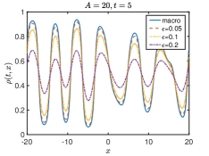
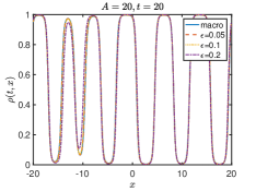
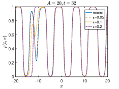
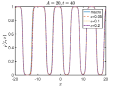
Figure 1: Comparison of $\rho_{\textnormal{macro}}$ and $\rho_{\textnormal{kinetic}}^{\varepsilon}$ for $A=20$ and different $\varepsilon$’s.

In Figure 2, we show the evolution of the energy quantities $\mathcal{E}(t)$ given by (35) (blue curve) and $\mathcal{E}_{\varepsilon}(t)$ as functions of time, for different values of $\varepsilon$: $\varepsilon=0.2$ (purple curve), $\varepsilon=0.1$ (yellow curve) and $\varepsilon=0.05$ (red curve), up to $t=50$. This figure shows that the energies of the kinetic and macroscopic models are in very good agreement. The inset figures show the evolution in time of the macroscopic density (continuous blue line) and the kinetic density for different values of $\varepsilon$ (lines with the same style as for the energy). It is clear from these figures that the larger discrepancies between the kinetic and macro energies are indeed related with changes in the density profiles, for example when two aggregates merge together (see the inset plots at $t=5$ and $t=32$). Even in this critical case of aggregation formation we observe that the kinetic solution for $\varepsilon=0.05$ agrees with the macroscopic solution.

A similar behaviour is observed in Figure 3 (left) where we plot the relative $L_{2}$-error between the kinetic and the macroscopic solutions as a function of time and for different values of $\varepsilon$ ($\varepsilon=0.2$, black curve, $\varepsilon=0.1$, blue curve and $\varepsilon=0.05$, red curve). In agreement with the behaviour observed in Figure 2 this error is larger at times $t=5$ and $t=32$, approximately, which corresponds to times where aggregates are merging.

In Figure 3 (right) we show the rate of convergence of the relative $L_{2}$-error between the kinetic, $\rho_{\textnormal{kinetic}}^{\varepsilon}$, and macroscopic, $\rho_{\textnormal{macro}}$, solutions for different values of $\varepsilon$, at different times. We observe that the error between both solutions decreases as $\varepsilon$ decreases, and the convergence order is around 1.5 in $\ell^{2}$ norm. Altogether, these first results suggest that the macroscopic and kinetic models are in good agreement for small values of $\varepsilon$, and that the kinetic model converges towards the macroscopic model as $\varepsilon\rightarrow 0$ in the 1D case. In Figure 3 (left) the kinetic model seems to converge faster to the “aggregated-state” compared to the macroscopic dynamics i.e. for large values of $\varepsilon$ (black curve) we see an early merging of aggregates, compared to the blue and red curves. These changes in speed could be due to the diffusion scaling, in which the macroscopic model is obtained in a regime where there are many velocity jumps but small net displacements in one order of time. Therefore, in the macroscopic setting, each particle interacts with many more particles than in the kinetic model, which could result in a delay in the aggregation process. In the next section, we take a step further and analyse the evolution of the pattern sizes in time as function of the chemotactic sensitivity $A$.

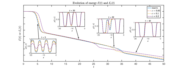
Figure 2: Evolution of $\mathcal{E}(t)$ and $\mathcal{E}_{\varepsilon}(t)$ along with the comparison between the kinetic solutions $\rho_{\textnormal{kinetic}}^{\varepsilon}$ and the macroscopic solutions $\rho_{\textnormal{macro}}(t,x)$ at $t=5,\ 20,\ 32,\ 40$ for $A=20$.

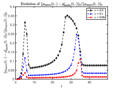
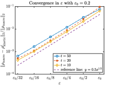
Figure 3: Left: Evolution of the relative $L_{2}$-error $\frac{\|\rho_{\rm{macro}}(t,\cdot)-\rho_{\rm{kinetic}}(t,\cdot)\|_{2}}{\|\rho_{\rm{macro}}(t,\cdot)\|}$ over time with $A=20$. Right: Convergence of the relative $L_{2}$-error in $\varepsilon$ at $t=10,\ 20,\ 50$. The numerical setting is the same as in Figure 1.

5.2 Pattern formation from a perturbed 1D initial data

With a strong chemotaxis effect, cells will aggregate to form patterns in regions where the chemoattractant is highly concentrated. For the volume-exclusion Keller-Segel model (20), a relation between the aggregate size from a perturbed initial data and the strength of chemotaxis effect $A$ was proven in [1] via linear stability analysis. In this section, we numerically verify this relation for both the kinetic (16) and the macroscopic model (20). Again, we only consider here the 1D case with periodic boundary conditions in space. More specifically, we consider the domain $(x,v)\in(-20,20)^{2}$ with a uniform mesh $\Delta x=0.1,\ \Delta v=0.2$. We choose the time step $\Delta t=10^{-3}$ and starting from a randomly perturbed initial data

$$\rho_{0_{\textnormal{macro}}}(t,x)=\rho_{0_{\textnormal{kinetic}}}^{\varepsilon}(t,x)=0.5+u(x)\ ,$$

we let the simulation run until $t=20$. To avoid effects due to the randomness of the initial data, we will compute the pattern size for 10 solutions, each evolved from some random initial data, and simply average.

To numerically compute the pattern sizes, we consider the Fourier transform of the density function $\rho(t,x)$ (macro and kinetic) and extract the frequency that corresponds to the maximal Fourier mode. Specifically, we consider

$$k_{\rm max}=\rm{argmax}_{\lambda}(|\hat{\rho}(\lambda)|)\ ,$$

where $\hat{\rho}(\lambda)=\mathcal{F}(\rho)(t,x)$ is the Fourier transform of the density function $\rho(t,x)$. Then, $1/k_{\rm max}$ can be used to describe the pattern size.

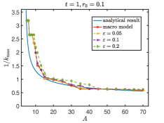
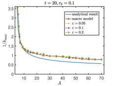
Figure 4: Comparison of $\frac{1}{k_{\textnormal{max}}}$ between the analytical, the numerical results of the macro and the kinetic model. The numerical result is computed by averaging 10 solutions, each evolved from a random initial data around $0.5$.

In Figure 4 we show the overall pattern sizes $1/k_{\rm max}$ as a function of the chemotaxis sensitivity $A$ at times $t=1$ (left panel) and $t=20$ (right panel). For each time, we plot the analytical prediction of $\frac{1}{k_{\max}}$ (blue line, see [1]), the numerical result for the macroscopic model (red line) and the results for the kinetic model with various values of $\varepsilon$ ($\varepsilon=0.05$ in yellow, $\varepsilon=0.1$ in purple and $\varepsilon=0.2$ in green lines). As one can observe, we obtain a very good agreement between the predicted pattern sizes and the ones computed numerically for both the macroscopic and kinetic models. As predicted by the stability analysis performed in [1], the pattern sizes decrease as the chemotactic sensitivity $A$ increases, and we recover the critical value $A^{*}\approx 6.9$ bellow which there are no patterns, i.e for which the perturbations are damped and the solution comes back to a homogeneous distribution.

5.3 2D numerical examples

The numerical schemes for both the kinetic model (23) and the macroscopic model (30) can be generalized to multi-dimensional problems, where the tensor-product grid is adopted (see Appendix B for a detailed description of the 2D numerical scheme for the kinetic model).

In this section we perform 2D simulations for both the kinetic model (20) and the volume-exclusion Keller-Segel model (16). We consider the computation domain $\Omega_{\mathbf{x}}=\{\mathbf{x}=(x_{1},x_{2})\in\mathbb{R}^{2}:-20\leq x_{1},x_{2}\leq 20\}$ with a uniform mesh $\Delta x_{1}=\Delta x_{2}=0.1$ and periodic boundary conditions. For the kinetic model (16) we need to further define the domain of the velocity $\Omega_{\mathbf{v}}=\{\mathbf{v}=(v_{1},v_{2})\in\mathbb{R}^{2}:-10\leq v_{1},v_{2}\leq 10\}$ with a uniform mesh $\Delta v_{1}=\Delta v_{2}=0.2$ and zero boundary conditions. We choose $r_{0}=0.1$, $\rho_{\rm max}=0.5$, $\bar{\rho}=1$ and

$$\psi_{0}(\mathbf{v})=\frac{1}{2\pi}e^{-\frac{|\mathbf{v}|^{2}}{2}},\quad\psi_{1}(\mathbf{v}\ ,\nabla_{\mathbf{x}}c)=\frac{\mathbf{v}}{2\pi}e^{-\frac{|\mathbf{v}|^{2}}{2}}\cdot\nabla_{\mathbf{x}}c\ .$$

As in the 1D case, we can check that the choices of $\psi_{0}(\mathbf{v})$ and $\psi_{1}(\mathbf{v})$ satisfy the Hypotheses H1 and H2.

We fix $\Delta t=10^{-2}$ and choose the initial data to be

$$\rho_{0_{\textnormal{macro}}}(\mathbf{x})=\rho_{0_{\textnormal{kinetic}}}^{\varepsilon}(\mathbf{x})=0.5+u(x)\ ,\quad c_{0}(\mathbf{x})=c_{0}^{\varepsilon}(\mathbf{x})=0.5\ ,$$

where $u(x)$ is a randomly chosen uniformly distributed function ranging in $(-0.1,0.1)$. In Figure 5 we show the numerical results at $t=5$ (first row), $t=20$ (second row) and $t=50$ (third row) for the macroscopic model with different chemotaxis sensitivities $A=6$ (first column), $A=20$ (second column) and $A=50$ (third column). As one can observe, starting from an initial data perturbed around the homogeneous value $0.5$, we obtain the formation of labyrinthic patterns for a chemotactic sensitivity $A>6$ (middle and right columns), while the solution dampens to the homogeneous state for $A=6$ (left column), in agreement with the predictions of the stability analysis performed in [1] and the results in Figure 4. Moreover, we observe that larger values of the chemotactic sensitivity $A$ leads to sharper layers near the boundary of the patterns (compare middle and right columns) as expected.

In Figure 6 we compare the solutions of the macroscopic 2D model (top row) with the solutions of the 2D kinetic model for $\varepsilon=10^{-2}$ (bottom row), for two values of the chemotactic sensitivity $A=20$ (first and third columns) and $A=50$ (second and fourth columns), and for different values of the initial data $\rho_{0}$: $\rho_{0}=0.5$ (first two columns) and $\rho_{0}=0.1$ (last two columns). As observed in [26], we recover the formation of different types of patterns as a function of the initial condition for both the kinetic and the macro solution, i.e. labyrinthic patterns in the case $\rho_{0}=0.5$ and round patterns for $\rho_{0}=0.1$ (compare the first two columns with the last two). Moreover, we observe that the pattern sizes decrease and become sharper when the chemotactic sensitivity $A$ increases also for the kinetic solution.

In order to quantify the differences between the kinetic and macroscopic 2D models, we show in Figure 7 (left) the evolution in time of the relative $L^{2}$-error between the macroscopic and kinetic models for different values of $\varepsilon$: $\varepsilon=10^{-2}$ (blue curve), $\varepsilon=10^{-4}$ (red curve), $\varepsilon=10^{-6}$ (yellow curve), $\varepsilon=10^{-8}$ (purple curve), and Figure 7 (right) shows this relative error as function of $\varepsilon$ for different time points: $t=1$ (blue curve), $t=3$ (red curve), $t=5$ (yellow curve) and $t=10$ (purple curve). We observe that the relative error between both models decreases as $\varepsilon$ decreases, and the reference line $y=x$ (green curve) shows that the rate of convergence of the kinetic model towards the macroscopic one is roughly $\mathcal{O}(\varepsilon)$.

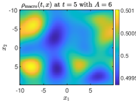
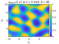
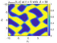
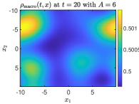
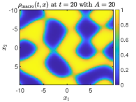
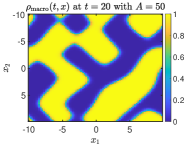
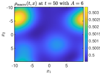
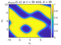
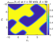
Figure 5: Plots of density $\rho_{\textnormal{macro}}(t,\mathbf{x})$ at $t=5,\ 20,\ 50$ (from top to bottom) with $A=6,\ 20,\ 50$ (from left to right), respectively.

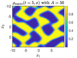
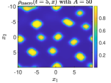
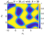
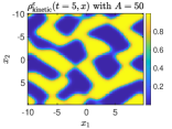
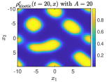
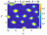
Figure 6: Comparison between $\rho_{\textnormal{macro}}(t,{\mathbf{x}})$ (first row) and $\rho_{\textnormal{kinetic}}^{\varepsilon}(t,{\mathbf{x}})$ with $\varepsilon=10^{-2}$ (second row) for different initial conditions $\rho_{0}\approx 0.5$ (first two columns) and $\rho_{0}\approx 0.1$ (last two columns) and different values of the chemotactic sensitivity $A=20$, (columns 1 and 3) and $A=50$ (columns 2 and 4).

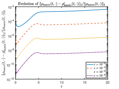
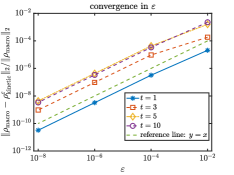
Figure 7: Left: Evolution of the relative $L_{2}$-error. Right: Convergence of the relative $L_{2}$-error in $\varepsilon$ at $t=1,\ 3,\ 5,\ 10$ with $A=20$ and $\Delta t=10^{-2}$.

6 Conclusions

In this paper we have derived a model for chemotaxis incorporating a density dependence in the chemotactic sensitivity function that takes into account the finite size of the cells and volume limitations. We showed, with formal arguments, that the macroscopic chemotactic system can be seen as the diffusion limit of a kinetic ’velocity-jump’ model, provided that both the transport term and the turning operator are density dependent. This derivation provides a more direct interpretation of the diffusion tensor and chemotactic sensitivity in terms of more fundamental characteristics of the motion.

We further studied this macroscopic limit numerically using an asymptotic preserving finite difference scheme based on a micro-macro decomposition of the unknown in the sense of [21], a projection technique to obtain a coupled system of two evolution equations for the microscopic and macroscopic components, and a suitable semi-implicit time discretization. The scheme was successfully extended to account for nonlinear terms by implicit-explicit discretization in an upwind manner, allowing for accurate approximations in the case of strong chemosensitivity. This scheme enabled us to explore numerically the different behaviours observed by the kinetic and macroscopic models in 1D and 2D, and we showed that both models are in good agreement as the diffusion scaling parameter becomes smaller. Moreover, the numerical simulations of the kinetic model revealed the same pattern sizes as obtained with the macroscopic model and predicted theoretically, with very good precision as $\varepsilon$ goes to zero in the kinetic setting. It is noteworthy that both models also feature the same dynamics in time, with a slight delay in the macroscopic simulations compared to the kinetic dynamics. This could be due to the fact that the macroscopic model is obtained in a regime where there are many velocity jumps but small net displacements in one order of time. Therefore, in the macroscopic setting, each particle interacts with many more particles than in the kinetic model, which could result in a delay in the aggregation process.

From the modelling perspective, it would be natural to extend the derivation to consider different turning kernels, to take into account cell-cell adhesion or nonlocal movement, for instance. The idea to construct the scheme could be generalized to include these cases, but we stress the fact that the detailed discretization is problem-dependent. Moreover, the rigorous derivation of volume-filling chemotactic equations from stochastic processes of interacting populations could be considered by adapting ideas from [29] for instance.

Appendix A Energy dissipation in the macroscopic model

Under proper assumptions, the macroscopic volume-exclusion Keller-Segel model (7) can be proven to be energy dissipate, which will be a key feature to be preserved in numerical methods. Following a gradient flow approach to energy in the sense of [5, 6, 8], we start by defining $H(\rho)=\frac{D_{0}}{\beta}\ln\left(\frac{\rho}{q(\rho)}\right)$. Then the volume-exclusion Keller-Segel model (7) can be reformulated as

$$\partial_{t}\rho+\nabla\cdot(\chi(\rho)\rho(-H^{\prime}(\rho)\nabla\rho+\nabla c))=0\ ,$$ (37)

where $\chi(\rho)=\beta q(\rho),\,H^{\prime}(\rho)=D_{0}\frac{q(\rho)-\rho q^{\prime}(\rho)}{\beta q(\rho)\rho}$. The energy functional of the model can be given by

$$\mathcal{E}(t)=\int\Phi(\rho)\mathop{}\!\mathrm{d}x-\frac{1}{2}\int\rho c\mathop{}\!\mathrm{d}x\ ,$$ (38)

where

$$\Phi^{\prime}(\rho)=H(\rho)\ .$$ (39)

Proposition 5.

Suppose that $\rho(t,\mathbf{x})$ and $c(t,\mathbf{x})$ solves the macroscopic volume-exclusion Keller-Segel equation (37) coupled with the equation

$$\Delta c+\rho-c=0\ ,$$ (40)

we have

$$\frac{\mathop{}\!\mathrm{d}}{\mathop{}\!\mathrm{d}t}\mathcal{E}(t)=-\int\rho\chi(\rho)|\nabla(H-c)|^{2}\mathop{}\!\mathrm{d}x\leq 0\ ,$$ (41)

where the energy functional $\mathcal{E}(t)$ is given by (38).

Proof.

Multiplying (37) by $H-c$, we get

$$(H-c)\partial_{t}\rho =(H-c)\nabla\cdot(\chi(\rho)\rho\nabla(H-c))$$

$$=\frac{1}{2}\nabla\cdot\left(\chi(\rho)\rho\nabla(H-c)^{2}\right)-\chi(\rho)\rho|\nabla(H-c)|^{2}\ ,$$

where we used the relation $H^{\prime}(\rho)\nabla\rho-\nabla c=\nabla(H-c)$. Then

$$\frac{\mathop{}\!\mathrm{d}}{\mathop{}\!\mathrm{d}t}\mathcal{E}(t) =\frac{\mathop{}\!\mathrm{d}}{\mathop{}\!\mathrm{d}t}\int\left(\Phi-\frac{1}{2}\rho c\right)\mathop{}\!\mathrm{d}x=\frac{\mathop{}\!\mathrm{d}}{\mathop{}\!\mathrm{d}t}\left[\int\left(\Phi-\frac{1}{2}c^{2}-\frac{1}{2}|\nabla c|^{2}\right)\mathop{}\!\mathrm{d}x\right]$$

$$=\int\left[H\partial_{t}\rho-c\left(\partial_{t}c-\Delta(\partial_{t}c)\right)\right]\mathop{}\!\mathrm{d}x=\int(H-c)\partial_{t}\rho\mathop{}\!\mathrm{d}x$$

$$=-\int\rho\chi(\rho)|\nabla(H-c)|^{2}\mathop{}\!\mathrm{d}x\leq 0\ .$$

∎

Remark 6.

Proposition 5 can be generalized to the equation

$$\partial_{t}\rho-\nabla\cdot(\chi(\rho)\rho(-H^{\prime}(\rho)\nabla\rho+\nabla c))=r_{0}\rho\left(1-\frac{\rho}{\rho_{\rm max}}\right)_{+},$$

where a proliferation term is included satisfying $\rho_{\rm max}+\frac{\rho_{\rm max}}{\bar{\rho}}\leq 1$. In fact, it can be checked that, when $\rho<\rho_{\rm max}$, we have $\rho<q(\rho)$ and thus $H<0$. The conclusion is then obvious.

Appendix B A finite difference scheme for the 2D kinetic model

The finite difference scheme (23) can be generalized to multi-dimensional problems where a tensor product grid is applied. Here we consider the 2D kinetic model with the special choice $\vec{\psi}_{1}=\vec{\phi}(v_{1},v_{2})\cdot\nabla c$, where $\vec{\phi}(v_{1},v_{2})=(\phi_{1}(v_{1},v_{2}),\phi_{2}(v_{1},v_{2}))^{T}$.

Denoting $\rho_{j_{1},j_{2}}^{n}$, $c_{j_{1},j_{2}}^{n}$, $g_{j_{1}+\frac{1}{2},j_{2},k_{1},k_{2}}^{(1),n}$ and $g_{j_{1},j_{2}+\frac{1}{2},k_{1},k_{2}}^{(2),n}$ to be the numerical approximations of $\rho(t_{n},x_{j_{1}},x_{j_{2}})$, $c(t_{n},x_{j_{1}},x_{j_{2}})$, $g(t_{n},x_{j_{1}+\frac{1}{2}},x_{j_{2}},v_{k_{1}},v_{k_{2}})$ and $g(t_{n},x_{j_{1}},x_{j_{2}+\frac{1}{2}},v_{k_{1}},v_{k_{2}})$, respectively. The approximations of $\rho(t,\mathbf{x})$ at half grid points such as $(x_{j_{1}},x_{j_{2}+\frac{1}{2}})$ can be then easily approximated by the average $\bar{\rho}_{j_{1},j_{2}+\frac{1}{2}}:=(\rho_{j_{1},j_{2}}+\rho_{j_{1},j_{2}+1})/2$. It is worth noticing that we used different notations for approximating $g(t_{n},x_{j_{1}+\frac{1}{2}},x_{j_{2}},*,*)$ and $g(t_{n},x_{j_{1}},x_{j_{2}+\frac{1}{2}},*,*)$ since different upwind discretizations will be used depending on whether the half grid is in $x_{1}$-direction or $x_{2}$-direction. An illustration of the grids in $\mathbf{x}$-space for computing $\rho(t,\mathbf{x})$ and $g(t,\mathbf{x},\mathbf{v})$ in 1D and 2D can be found in Figure 8.

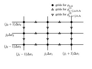
Figure 8: Illustration of the grids in $\mathbf{x}$-space for computing $\rho(t,\mathbf{x})$ and $g(t,\mathbf{x},\mathbf{v})$ in 1D and 2D.

With the notations defined, the 2D kinetic model (16) can be discretized as

$$\begin{cases}&\delta_{t}^{+}\rho_{j_{1},j_{2}}^{n}+\sum_{k_{1},k_{2}}\left[v_{k_{1}}\delta_{x_{1}}(q({\rho}_{*,j_{2}}^{n})g_{*,j_{2},k_{1},k_{2}}^{(1),n+1})_{j_{1}}+v_{k_{2}}\delta_{x_{2}}(q({\rho}_{j_{1},*}^{n})g_{j_{1},*,k_{1},k_{2}}^{(2),n+1})_{j_{2}}\right]\Delta v_{1}\Delta v_{2}\\ &\quad+D_{h}\left[\delta_{x_{1}}({\rho}_{*,j_{2}}^{n}q^{\prime}({\rho}_{*,j_{2}}^{n})\delta_{x_{1}}\rho_{*,j_{2}}^{n+1})_{j_{1}}+\delta_{x_{2}}({\rho}_{j_{1},*}^{n}q^{\prime}({\rho}_{j_{1},*}^{n})\delta_{x_{2}}\rho_{j_{1},*}^{n+1})_{j_{2}}\right]=r_{0}\rho_{j_{1},j_{2}}^{n}\left(1-\frac{\rho_{j_{1},j_{2}}^{n}}{\rho_{\rm max}}\right)_{+},\\ &\delta_{t}^{+}g_{j_{1}+\frac{1}{2},j_{2},k_{1},k_{2}}^{(1),n}+\frac{1}{\varepsilon}(I-\Pi_{h})K_{j_{1}+\frac{1}{2},j_{2},k_{1},k_{2}}^{(1),n}=\frac{1}{\varepsilon^{2}}S_{j_{1}+\frac{1}{2},j_{2},k_{1},k_{2}}^{(1),n,n+1}+r_{0}g_{j_{1}+\frac{1}{2},j_{2},k_{1},k_{2}}^{(1),n}\left(1-\frac{\rho_{j_{1}+\frac{1}{2},j_{2}}^{n}}{\rho_{\rm max}}\right)_{+},\\ &\delta_{t}^{+}g_{j_{1},j_{2}+\frac{1}{2},k_{1},k_{2}}^{(2),n}+\frac{1}{\varepsilon}(I-\Pi_{h})K_{j_{1},j_{2}+\frac{1}{2},k_{1},k_{2}}^{(2),n}=\frac{1}{\varepsilon^{2}}S_{j_{1},j_{2}+\frac{1}{2},k_{1},k_{2}}^{(2),n,n+1}+r_{0}g_{j_{1},j_{2}+\frac{1}{2},k_{1},k_{2}}^{(2),n}\left(1-\frac{\rho_{j_{1},j_{2}+\frac{1}{2}}^{n}}{\rho_{\rm max}}\right)_{+},\\ &(\delta_{x_{1}}^{2}+\delta_{x_{2}}^{2})c_{j_{1},j_{2}}^{n+1}+\rho_{j_{1},j_{2}}^{n+1}-c_{j_{1},j_{2}}^{n+1}=0,\end{cases}$$ (42)

where $\Pi_{h}$ is the discrete projection operator defined as

$$\Pi_{h}\eta_{j_{1},j_{2},k_{1},k_{2}}^{n}=\sum_{k_{1},k_{2}}\eta_{j_{1},j_{2},k_{1},k_{2}}^{n}\psi_{0}(v_{k_{1}},v_{k_{2}})\Delta v_{1}\Delta v_{2}$$

for some general function $\eta(t,\mathbf{x},\mathbf{v})$ and

$$K_{j_{1}+\frac{1}{2},j_{2},k_{1},k_{2}}^{(1),n}=v_{k_{1}}^{+}\delta_{x_{1}}(q({\rho}_{*,j_{2}}^{n})g_{*,j_{2},k_{1},k_{2}}^{(1),n})_{j_{1}}-v_{k_{1}}^{-}\delta_{x_{1}}(q({\rho}_{*,j_{2}}^{n})g_{*,j_{2},k_{1},k_{2}}^{(1),n})_{j_{1}+1}$$

$$\qquad+v_{k_{2}}^{+}\delta_{x_{2}}(q({\rho}_{j_{1}+\frac{1}{2},*}^{n})g_{j_{1}+\frac{1}{2},*,k_{1},k_{2}}^{(1),n})_{j_{2}-\frac{1}{2}}-v_{k_{2}}^{-}\delta_{x_{2}}(q({\rho}_{j_{1}+\frac{1}{2},*}^{n})g_{j_{1}+\frac{1}{2},*,k_{1},k_{2}}^{(1),n})_{j_{2}+\frac{1}{2}}$$

$$\qquad+\psi_{0}(v_{k_{1}},v_{k_{2}})\delta_{x_{1}}\left\{{\rho}_{*,j_{2}}^{n}q^{\prime}({\rho}_{*,j_{2}}^{n})\left[v_{k_{1}}^{2}\delta_{x_{1}}\rho_{*,j_{2}}^{n}+v_{k_{1}}v_{k_{2}}(\delta_{x_{2}}\rho_{*,**}^{n})_{j_{2}}\right]\right\}_{j_{1}+\frac{1}{2}}\ ,$$

$$\qquad+\psi_{0}(v_{k_{1}},v_{k_{2}})\delta_{x_{2}}\left\{{\rho}_{j_{1}+\frac{1}{2},*}^{n}q^{\prime}({\rho}_{j_{1}+\frac{1}{2},*}^{n})\left[v_{k_{1}}v_{k_{2}}(\delta_{x_{1}}\rho_{**,*}^{n})_{j_{1}+\frac{1}{2}}+v_{k_{2}}^{2}\delta_{x_{2}}\rho_{j_{1}+\frac{1}{2},*}^{n}\right]\right\}_{j_{2}}\ ,$$

$$K_{j_{1},j_{2}+\frac{1}{2},k_{1},k_{2}}^{(2),n}=v_{k_{1}}^{+}\delta_{x_{1}}(q({\rho}_{*,j_{2}+\frac{1}{2}}^{n})g_{*,j_{2}+\frac{1}{2},k_{1},k_{2}}^{(1),n})_{j_{1}-\frac{1}{2}}-v_{k_{1}}^{-}\delta_{x_{1}}(q({\rho}_{*,j_{2}+\frac{1}{2}}^{n})g_{*,j_{2}+\frac{1}{2},k_{1},k_{2}}^{(1),n})_{j_{1}+\frac{1}{2}}$$

$$\qquad+v_{k_{2}}^{+}\delta_{x_{2}}(q({\rho}_{j_{1},*}^{n})g_{j_{1},*,k_{1},k_{2}}^{(1),n})_{j_{2}}-v_{k_{2}}^{-}\delta_{x_{2}}(q({\rho}_{j_{1},*}^{n})g_{j_{1},*,k_{1},k_{2}}^{(1),n})_{j_{2}+1}$$

$$\qquad+\psi_{0}(v_{k_{1}},v_{k_{2}})\delta_{x_{1}}\left\{{\rho}_{*,j_{2}+\frac{1}{2}}^{n}q^{\prime}({\rho}_{*,j_{2}+\frac{1}{2}}^{n})\left[v_{k_{1}}^{2}\delta_{x_{1}}\rho_{*,j_{2}+\frac{1}{2}}^{n}+v_{k_{1}}v_{k_{2}}(\delta_{x_{2}}\rho_{*,**}^{n})_{j_{2}+\frac{1}{2}}\right]\right\}_{j_{1}}\ ,$$

$$\qquad+\psi_{0}(v_{k_{1}},v_{k_{2}})\delta_{x_{2}}\left\{{\rho}_{j_{1},*}^{n}q^{\prime}({\rho}_{j_{1},*}^{n})\left[v_{k_{1}}v_{k_{2}}(\delta_{x_{1}}\rho_{**,*}^{n})_{j_{1}}+v_{k_{2}}^{2}\delta_{x_{2}}\rho_{j_{1},*}^{n}\right]\right\}_{j_{2}+\frac{1}{2}}\ ,$$

$$S_{j_{1}+\frac{1}{2},j_{2},k_{1},k_{2}}^{(1),n,n+1}=-\psi_{0}(v_{k_{1}},v_{k_{2}})q({\rho}_{j_{1}+\frac{1}{2},j_{2}}^{n})\left[v_{k_{1}}\delta_{x_{1}}\rho_{j_{1}+\frac{1}{2},j_{2}}^{n+1}+v_{k_{2}}\delta_{x_{2}}\rho_{j_{1}+\frac{1}{2},j_{2}}^{n+1}\right]$$

$$\qquad+\phi_{1}(v_{k_{1}},v_{k_{2}})\delta_{x_{1}}c_{j_{1}+\frac{1}{2},j_{2}}^{n}\Phi^{(1),n+1,n}_{j_{1}+\frac{1}{2},j_{2}}+\phi_{2}(v_{k_{1}},v_{k_{2}})\delta_{x_{2}}c_{j_{1}+\frac{1}{2},j_{2}}^{n}\Phi^{(2),n+1,n}_{j_{1}+\frac{1}{2},j_{2}}-q({\rho}_{j_{1}+\frac{1}{2},j_{2}}^{n})g_{j_{1}+\frac{1}{2},j_{2},k_{1},k_{2}}^{(1),n+1}\ ,$$

$$S_{j_{1},j_{2}+\frac{1}{2},k_{1},k_{2}}^{(2),n,n+1}=-\psi_{0}(v_{k_{1}},v_{k_{2}})q({\rho}_{j_{1},j_{2}+\frac{1}{2}}^{n})\left[v_{k_{1}}\delta_{x_{1}}\rho_{j_{1},j_{2}+\frac{1}{2}}^{n+1}+v_{k_{2}}\delta_{x_{2}}\rho_{j_{1},j_{2}+\frac{1}{2}}^{n+1}\right]$$

$$\qquad+\phi_{1}(v_{k_{1}},v_{k_{2}})\delta_{x_{1}}c_{j_{1},j_{2}+\frac{1}{2}}^{n}\Phi^{(1),n+1,n}_{j_{1},j_{2}+\frac{1}{2}}+\phi_{2}(v_{k_{1}},v_{k_{2}})\delta_{x_{2}}c_{j_{1},j_{2}+\frac{1}{2}}^{n}\Phi^{(2),n+1,n}_{j_{1},j_{2}+\frac{1}{2}}-q({\rho}_{j_{1},j_{2}+\frac{1}{2}}^{n})g_{j_{1},j_{2}+\frac{1}{2},k_{1},k_{2}}^{(2),n+1}\ ,$$

where, as in the 1D case, both $\Phi^{(1),n_{1},n}$ and $\Phi^{(1),n_{1},n}$ are upwind approximations of $q(\rho)\rho$ at $t=t_{n}$ and defined as

$$\Phi^{(1),n_{1},n}_{j_{1},j_{2}}=\begin{cases}\rho_{j_{1}-\frac{1}{2},j_{2}}^{n_{1}}q(\rho_{j_{1}+\frac{1}{2},j_{2}}^{n})\ ,\quad&\text{ if }\delta_{x_{1}}c_{j_{1},j_{2}}^{n}\geq 0\ ,\\ \rho_{j_{1}+\frac{1}{2},j_{2}}^{n_{1}}q(\rho_{j_{1}-\frac{1}{2},j_{2}}^{n})\ ,\quad&\text{ if }\delta_{x_{1}}c_{j_{1},j_{2}}^{n}<0\ ,\end{cases}$$

$$\Phi^{(2),n_{1},n}_{j_{1},j_{2}}=\begin{cases}\rho_{j_{1},j_{2}-\frac{1}{2}}^{n_{1}}q(\rho_{j_{1},j_{2}+\frac{1}{2}}^{n})\ ,\quad&\text{ if }\delta_{x_{2}}c_{j_{1},j_{2}}^{n}\geq 0\ ,\\ \rho_{j_{1},j_{2}+\frac{1}{2}}^{n_{1}}q(\rho_{j_{1},j_{2}-\frac{1}{2}}^{n})\ ,\quad&\text{ if }\delta_{x_{2}}c_{j_{1},j_{2}}^{n}<0\ ,\end{cases}$$

As for the 1D case, we can formally prove the asymptotic preserving property of the 2D scheme (42) in a similar way. In fact, when $\varepsilon\to 0$, we expect that

$$S_{j_{1}+\frac{1}{2},j_{2},k_{1},k_{2}}^{(1),n,n+1}=0\ ,\qquad S_{j_{1},j_{2}+\frac{1}{2},k_{1},k_{2}}^{(2),n,n+1}=0,$$

from where we get

$$q({\rho}_{j_{1}+\frac{1}{2},j_{2}}^{n})g_{j_{1}+\frac{1}{2},j_{2},k_{1},k_{2}}^{(1),n+1}=-\psi_{0}(v_{k_{1}},v_{k_{2}})q({\rho}_{j_{1}+\frac{1}{2},j_{2}}^{n})\left[v_{k_{1}}\delta_{x_{1}}\rho_{j_{1}+\frac{1}{2},j_{2}}^{n+1}+v_{k_{2}}\delta_{x_{2}}\rho_{j_{1}+\frac{1}{2},j_{2}}^{n+1}\right]$$

$$\qquad+\phi_{1}(v_{k_{1}},v_{k_{2}})\delta_{x_{1}}c_{j_{1}+\frac{1}{2},j_{2}}^{n}\Phi^{(1),n+1,n}_{j_{1}+\frac{1}{2},j_{2}}+\phi_{2}(v_{k_{1}},v_{k_{2}})\delta_{x_{2}}c_{j_{1}+\frac{1}{2},j_{2}}^{n}\Phi^{(2),n+1,n}_{j_{1}+\frac{1}{2},j_{2}},$$

$$q({\rho}_{j_{1},j_{2}+\frac{1}{2}}^{n})g_{j_{1},j_{2}+\frac{1}{2},k_{1},k_{2}}^{(2),n+1}=-\psi_{0}(v_{k_{1}},v_{k_{2}})q({\rho}_{j_{1},j_{2}+\frac{1}{2}}^{n})\left[v_{k_{1}}\delta_{x_{1}}\rho_{j_{1},j_{2}+\frac{1}{2}}^{n+1}+v_{k_{2}}\delta_{x_{2}}\rho_{j_{1},j_{2}+\frac{1}{2}}^{n+1}\right]$$

$$\qquad+\phi_{1}(v_{k_{1}},v_{k_{2}})\delta_{x_{1}}c_{j_{1},j_{2}+\frac{1}{2}}^{n}\Phi^{(1),n+1,n}_{j_{1},j_{2}+\frac{1}{2}}+\phi_{2}(v_{k_{1}},v_{k_{2}})\delta_{x_{2}}c_{j_{1},j_{2}+\frac{1}{2}}^{n}\Phi^{(2),n+1,n}_{j_{1},j_{2}+\frac{1}{2}}\ .$$

Substituting into the first equation in (42) and using the fact that

$$\sum_{k_{1},k_{2}}v_{k_{i}}v_{k_{j}}\psi_{0}(v_{k_{1}},v_{k_{2}})\Delta v_{1}\Delta v_{2}=D_{h}\delta_{i,j}, \sum_{k_{1},k_{2}}v_{k_{i}}\phi_{j}(v_{k_{1}},v_{k_{2}})\Delta v_{1}\Delta v_{2}=A\delta_{i,j},\quad i,j=1,2,$$

we recover the finite difference scheme for the macro model

$$\delta_{t}^{+}\rho_{j_{1},j_{2}}^{n}-D_{h}\delta_{x_{1}}\left[(q(\rho_{*,j_{2}}^{n})-{\rho}_{*,j_{2}}^{n}q^{\prime}({\rho}_{*,j_{2}}^{n}))\delta_{x_{1}}\rho_{*,j_{2}}^{n+1}\right]_{j_{1}}-D_{h}\delta_{x_{2}}\left[(q(\rho_{j_{1},*}^{n})-{\rho}_{j_{1},*}^{n}q^{\prime}({\rho}_{j_{1},*}^{n}))\delta_{x_{2}}\rho_{j_{1},*}^{n+1}\right]_{j_{2}}$$

$$\quad+A\delta_{x_{1}}\left[\Phi_{*,j_{2}}^{(1),n+1,n}\delta_{x_{1}}c_{*,j_{2}}^{n}\right]_{j_{1}}+A\delta_{x_{2}}\left[\Phi_{j_{1},*}^{(1),n+1,n}\delta_{x_{2}}c_{j_{1},*}^{n}\right]_{j_{2}}=r_{0}\rho_{j_{1},j_{2}}^{n}\left(1-\frac{\rho_{j_{1},j_{2}}^{n}}{\rho_{\rm max}}\right)_{+}\ .$$

References

- [1] L. Almeida, G. Estrada-Rodriguez, L. Oliver, D. Peurichard, A. Poulain, and F. Vallette. Treatment-induced shrinking of tumour aggregates: A nonlinear volume-filling chemotactic approach. arXiv preprint arXiv:2007.12454, 2020.
- [2] W. Alt. Biased random walk models for chemotaxis and related diffusion approximations. Journal of mathematical biology, 9(2):147–177, 1980.
- [3] R. Bailo, J. A. Carrillo, and J. Hu. Fully discrete positivity-preserving and energy-dissipating schemes for aggregation-diffusion equations with a gradient-flow structure. Communications in Mathematical Sciences, 18(5):1259–1303, 2020.
- [4] F. Bubba, C. Pouchol, N. Ferrand, G. Vidal, L. Almeida, B. Perthame, and M. Sabbah. A chemotaxis-based explanation of spheroid formation in 3D cultures of breast cancer cells. Journal of theoretical biology, 479:73–80, 2019.
- [5] V. Calvez and J. A. Carrillo. Volume effects in the Keller–Segel model: energy estimates preventing blow-up. Journal de mathématiques pures et appliquées, 86(2):155–175, 2006.
- [6] J. A. Carrillo, A. Jüngel, P. A. Markowich, G. Toscani, and A. Unterreiter. Entropy dissipation methods for degenerate parabolic problems and generalized Sobolev inequalities. Monatshefte für Mathematik, 133(1):1–82, 2001.
- [7] J. A. Carrillo and B. Yan. An asymptotic preserving scheme for the diffusive limit of kinetic systems for chemotaxis. Multiscale Modeling & Simulation, 11(1):336–361, 2013.
- [8] L. N. De Almeida, F. Bubba, B. Perthame, and C. Pouchol. Energy and implicit discretization of the Fokker-Planck and Keller-Segel type equations. arXiv preprint arXiv:1803.10629, 2018.
- [9] Y. Dolak and C. Schmeiser. The Keller–Segel model with logistic sensitivity function and small diffusivity. SIAM Journal on Applied Mathematics, 66(1):286–308, 2005.
- [10] C. Emako and M. Tang. Well-balanced and asymptotic preserving schemes for kinetic models. arXiv preprint arXiv:1603.03171, 2016.
- [11] F. Filbet and S. Jin. A class of asymptotic-preserving schemes for kinetic equations and related problems with stiff sources. Journal of Computational Physics, 229(20):7625–7648, 2010.
- [12] Y. Han, Z. Li, J. Tao, and M. Ma. Pattern formation for a volume-filling chemotaxis model with logistic growth. Journal of Mathematical Analysis and Applications, 448(2):885–907, 2017.
- [13] T. Hillen and K. Painter. A user’s guide to PDE models for chemotaxis. J. Math. Biol, 58:183–217, 2009.
- [14] M. Ibrahim and M. Saad. On the efficacy of a control volume finite element method for the capture of patterns for a volume-filling chemotaxis model. Computers & Mathematics with Applications, 68(9):1032–1051, 2014.
- [15] S. Jin. Efficient asymptotic-preserving (AP) schemes for some multiscale kinetic equations. SIAM Journal on Scientific Computing, 21(2):441–454, 1999.
- [16] S. Jin and B. Yan. A class of asymptotic-preserving schemes for the Fokker–Planck–Landau equation. Journal of Computational Physics, 230(17):6420–6437, 2011.
- [17] T. Jin, X. Xu, and D. Hereld. Chemotaxis, chemokine receptors and human disease. Cytokine, 44(1):1–8, 2008.
- [18] U. B. Kaupp. 100 years of sperm chemotaxis. J Gen Physiol., 406(6):583–586, 2012.
- [19] E. F. Keller and L. A. Segel. Initiation of slime mold aggregation viewed as an instability. Journal of theoretical biology, 26(3):399–415, 1970.
- [20] E. F. Keller and L. A. Segel. Model for chemotaxis. Journal of theoretical biology, 30(2):225–234, 1971.
- [21] M. Lemou and L. Mieussens. A new asymptotic preserving scheme based on micro-macro formulation for linear kinetic equations in the diffusion limit. SIAM Journal on Scientific Computing, 31(1):334–368, 2008.
- [22] M. Ma, C. Ou, and Z.-A. Wang. Stationary solutions of a volume-filling chemotaxis model with logistic growth and their stability. SIAM Journal on Applied Mathematics, 72(3):740–766, 2012.
- [23] H. G. Othmer, S. R. Dunbar, and W. Alt. Models of dispersal in biological systems. Journal of mathematical biology, 26(3):263–298, 1988.
- [24] H. G. Othmer and T. Hillen. The diffusion limit of transport equations derived from velocity-jump processes. SIAM Journal on Applied Mathematics, 61(3):751–775, 2000.
- [25] H. G. Othmer and T. Hillen. The diffusion limit of transport equations ii: Chemotaxis equations. SIAM Journal on Applied Mathematics, 62(4):1222–1250, 2002.
- [26] K. J. Painter and T. Hillen. Volume-filling and quorum-sensing in models for chemosensitive movement. Can. Appl. Math. Quart, 10(4):501–543, 2002.
- [27] C. S. Patlak. Random walk with persistence and external bias. The bulletin of mathematical biophysics, 15(3):311–338, 1953.
- [28] E. Roussos, J. Condeelis, and A. Patsialou. Chemotaxis in cancer. Nat Rev Cancer, 11(8):573–587, 2011.
- [29] A. Stevens. The derivation of chemotaxis equations as limit dynamics of moderately interacting stochastic many-particle systems. SIAM Journal on Applied Mathematics, 61(1):183–212, 2000.
- [30] F. G. Vital-Lopez, A. Armaou, M. Hutnik, and C. D. Maranas. Modeling the effect of chemotaxis on glioblastoma tumor progression. AIChE Journal, 57(3):778–792, 2011.
- [31] L. Wang and B. Yan. An asymptotic-preserving scheme for the kinetic equation with anisotropic scattering: Heavy tail equilibrium and degenerate collision frequency. SIAM Journal on Scientific Computing, 41(1):A422–A451, 2019.
- [32] Z. Wang. On chemotaxis models with cell population interactions. Mathematical Modelling of Natural Phenomena, 5(3):173–190, 2010.
- [33] Z. Wang and T. Hillen. Classical solutions and pattern formation for a volume filling chemotaxis model. Chaos: An Interdisciplinary Journal of Nonlinear Science, 17(3):037108, 2007.
- [34] D. Wrzosek. Volume filling effect in modelling chemotaxis. Mathematical Modelling of Natural Phenomena, 5(1):123–147, 2010.
- [35] P. Zheng, C. Mu, and X. Hu. Boundedness and blow-up for a chemotaxis system with generalized volume-filling effect and logistic source. Discrete & Continuous Dynamical Systems, 35(5):2299, 2015.