The Mass-Metallicity Relation of Dwarf Galaxies at Cosmic Noon from JWST Observations

Abstract

We present a study of the mass-metallicity relation (MZR) of 51 dwarf galaxies ($M_{\star}\approx 10^{6.5}-10^{9.5}\mathrm{M}_{\odot}$) at $z=2-3$ from the Abell 2744 and SMACS J0723-3732 galaxy cluster fields. These dwarf galaxies are identified and confirmed by deep JWST/NIRISS imaging and slitless grism spectroscopic observations. By taking advantage of the superior performance of JWST and the gravitational lensing effect, we extend the previous MZR relation at $z=2-3$ to a much lower mass regime down by $\approx$ 2.5 orders of magnitude as compared with previous studies. We find that the MZR has a shallower slope at the low-mass end ($M_{\star}<10^{9}~{}\rm\mathrm{M}_{\odot}$), with a slope turnover point of $\approx$ $10^{9}~{}\rm\mathrm{M}_{\odot}$. This implies that the dominating feedback processes in dwarf galaxies may be different from that in massive galaxies. From $z=3$ to $z=2$, the metallicity of the dwarf galaxies is enhanced by $\approx 0.09$ dex for a given stellar mass, consistent with the mild evolution found in galaxies with higher mass. Furthermore, we confirm the existence of a fundamental metallicity relation (FMR) between the gas-phase metallicity, stellar mass, and star formation rate in dwarf galaxies at $z=2-3$. Our derived FMR, which has no significant redshift evolution, can be used as a benchmark to understand the origin of the anti-correlation between the SFR and metallicity of dwarf galaxies in the high-$z$ Universe.

1 Introduction

The mass-metallicity relation (MZR) is one of the most fundamental relations for quantifying the chemical enrichment and gas properties of star-forming galaxies and has been studied across cosmic time (e.g., Tremonti et al., 2004; Erb et al., 2006; Maier et al., 2014; Steidel et al., 2014; Sanders et al., 2015; Guo et al., 2016; Sanders et al., 2021; Papovich et al., 2022; Li et al., 2022). In this scaling relation, the metallicity increases with stellar mass, and galaxies at high redshifts tend to have lower metallicity than their low-redshift counterparts for a given stellar mass. The normalization, slope, and scatter of the MZR provide insight into the physical mechanisms regulating galaxy evolution, including how metals have been produced and driven out of galaxies and how pristine/metal-populated gas has been accreted into galaxies (e.g., Peeples & Shankar, 2011; Lilly et al., 2013; Torrey et al., 2019).

Dwarf galaxies are the most numerous type of observed galaxies. They are believed to dominate the ionizing photon budget and play the most important role in the metal enrichment of the circum-/intergalacitic medium (CGM/IGM) (e.g., Robertson et al., 2010; Lin et al., 2022; Wu et al., 2021), giving them great cosmological importance. Understanding the gas properties of dwarf galaxies and studying the evolution of gas-phase metallicity of dwarf galaxies at a given stellar mass can provide insight into the baryonic processes that regulate star formation and galaxy growth throughout cosmic history. Nevertheless, to date, most studies focus on the MZR of high to intermediate mass galaxies ($>$ 10⁹ $\mathrm{M}_{\odot}$). At these mass ranges, there have been multiple examples of the MZR at different redshifts haing similar slopes (e.g., Zahid et al., 2014; Sanders et al., 2021).

At low redshift, Zahid et al. (2012) studied the MZR $z\sim 0$ using a sample of local dwarf galaxies. They found that the scatter of MZR increases with decreasing stellar mass. Similarly, Guo et al. (2016) identified an increase in MZR scatter in a sample of dwarf galaxies at $0.5<z<0.7$ and tentatively suggested a shallower MZR slope when the stellar mass is lower than $10^{9}~{}\mathrm{M_{\odot}}$. However, the MZR has been probed in very few high-$z$ ($z>2$), low-mass galaxies ($<$ $10^{9}\mathrm{M}_{\odot}$). Therefore, it is unclear whether the MZR has the same slope at the low mass end and how the MZR for dwarf galaxies evolves with cosmic time beyond $z=2$.

In this paper, we probe the MZR in a sample of 51 dwarf galaxies ($M_{\star}\approx 10^{6.5}-10^{9.5}\ \mathrm{M}_{\odot}$) at $z=2-3$ using Near-Infrared Imager and Slitless Spectrograph (NIRISS) grism spectroscopy mounted on James Webb Space Telescope (JWST) in the Abell 2744 and SMACS J0723-3732 fields.

This paper is organized as follows. We briefly describe the observations, data, and sample selection in Section 2. In Section 3 we measure and derive the physical properties of our sample and we report the results of MZR for dwarf galaxies at $z=2-3$. We investigate the physical interpretation of the shape and evolution of MZR and discuss the existence of fundamental metallicity relation in Section 4. Throughout this paper, we use AB magnitudes (e.g., Oke & Gunn, 1983). We adopt a flat $\mathrm{\Lambda CDM}$ cosmology with $\Omega_{\mathrm{m}}=0.3$ and $H_{0}=70\mathrm{~{}km}\mathrm{~{}s}^{-1}\mathrm{~{}Mpc}^{-1}$ and a Chabrier (2003) Initial Mass Function (IMF).

2 Data and Sample

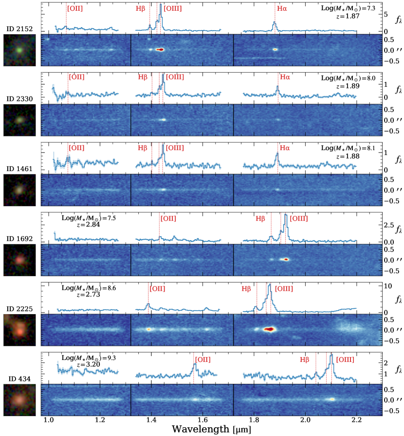
Figure 1(a): The $1.5\arcsec\times 1.5\arcsec$ RGB (red for JWST/NIRISS F200W, green for F150W, and blue for F115W) cutouts, extracted 1D spectra, and corresponding 2D spectra for six galaxies in our sample. Their IDs, redshifts, and stellar masses are labeled. The flux density of 1D spectra, $f_{\lambda}$, is in unit of $10^{-19}\mathrm{\,erg\,s^{-1}\,cm^{-2}\,\text{\AA}^{-1}}$.

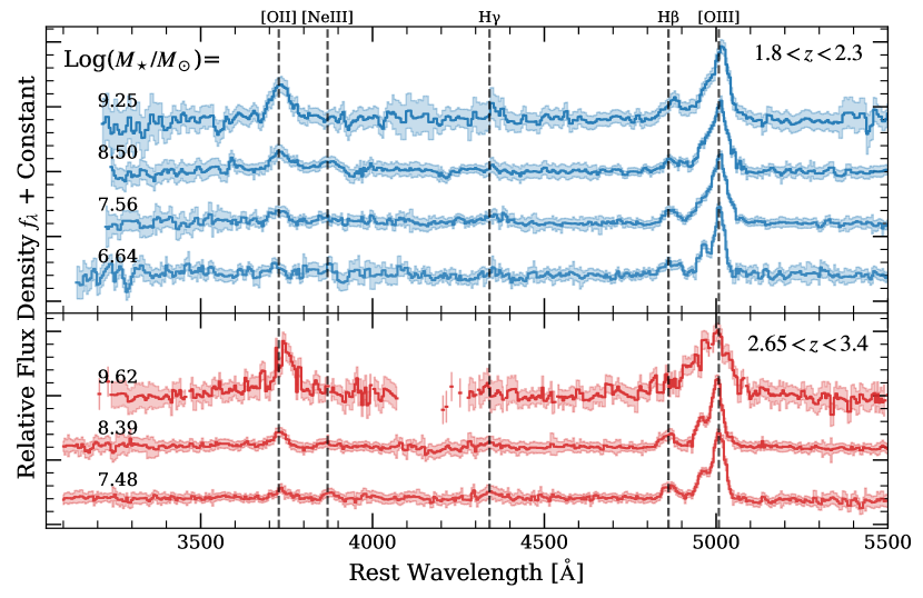
Figure 1(b): One-dimensional spectral stacks binned by redshift and stellar mass, with each individual continuum-subtracted spectrum normalized by a de-reddening flux of [O III] (see Section 3.3 for more details). The solid lines show the weighted average stacked spectra, and the shaded regions indicate the corresponding 1$\sigma$ uncertainties. The low S/N wavelength ranges located at the edge of filter bands are masked. Emission lines are labeled as black dashed lines. The [O III]/[O II] line ratio evolves prominently with the stellar mass, demonstrating that galaxies with lower stellar mass tend to be more metal-poor.

We create our galaxy sample in two cluster fields, Abell 2744 (A2744) field and SMACS J0723-3732 (SMACS 0723). These fields are extensively covered by JWST/NIRISS grism spectroscopy and imaging data from HST and JWST. The wavelength range (0.9 - 2.3 $\mu$m) of the JWST/NIRISS spectroscopy of these galaxies covers the metallicity diagnostics emission lines, including [O II], [O III], H$\beta$ at $z=2-3$. The high signal-to-noise (S/N) of JWST/NIRISS grism spectroscopy plus gravitational lensing allows us to detect the emission lines of galaxies with extraordinarily low stellar masses ($\approx$ $10^{6.5}\ \mathrm{M}_{\odot}$ at $z=2-3$). The complete coverage of the optical and IR imaging in SMACS 0723 (e.g., Pontoppidan et al., 2022; Coe et al., 2019) and A2744 fields (e.g., Treu et al., 2022; Lotz et al., 2017) also allows us to have an excellent estimate of the stellar mass down to $10^{6}\ \mathrm{M}_{\odot}$ at $z=2-3$, allowing for our measure of the MZR using a sample of dwarf galaxies at $z=2-3$.

2.1 JWST/NIRISS Grism Spectroscopic Observations

NIRISS observations of the A2744 field were taken by the GLASS JWST ERS program (ERS-1324: Treu et al., 2022). The integration time is $2835\mathrm{~{}s}$ ($\simeq 47\mathrm{\,minutes})$ for pre-imaging and $2\times 5196.5\mathrm{~{}s}~{}(\simeq 2.9\mathrm{\,hr})$ for GR150 row and column (R+C) grism with three filters (F115W, F150W, F200W). This observation setup provides almost continuous wavelength coverage from $1$ to $2.2\mathrm{~{}\mu m}$ in the A2744 field.

SMACS 0723 field was targeted by the JWST early-release observation program (ERO 2736: Pontoppidan et al., 2022). The JWST/NIRISS grism spectroscopy was obtained in F115W (1–1.3 µm) and F200W (1.7–2.2 µm) filters. The exposure time of the NIRISS grism observations of SMACS 0723 is $2\times 2834.5\mathrm{~{}s}~{}(\simeq 1.6\mathrm{~{}hr})$ for each filter, respectively.

The JWST data were reduced and calibrated following the methodology of Wu et al. (2022). The data were reduced using the standard JWST pipeline v1.9.4 with calibration reference files “jwst_1041.pmap”. First, we modeled the 1/f noise (see Schlawin et al. 2020) and removed it using the tshirt/roeba code. Then, we identified “snowball” artifacts from cosmic rays (Rigby et al., 2022a) and masked them. We then registered the world coordinate system of mosaicked images using the Pan-STARRS DR1 catalog (Flewelling et al., 2020) (Gaia DR2 catalog, Gaia Collaboration et al., 2018) for A2744 (SMACS 0723) field. Lastly, the pixel scale of final mosaicked images was resampled to 0.03″ with pixfrac $=$ 0.8. We reduced NIRISS grism data using the Grism Redshift & Line Analysis tool (Grizli; Brammer et al. 2022). The 2D grism spectra were drizzled with a pixel scale of 0.065″.

The JWST/NIRISS grism observations cover the metallicity-senstive lines [O II]$~{}\lambda\lambda 3727,3729$, H$\beta$, and [O III]$~{}\lambda\lambda 4959,5007$, allowing for our gas-phase oxygen abundance estimate. The spectral resolution ($R\equiv\lambda/\Delta\lambda$) of JWST/NIRISS observations is $\approx$150, enabling the separation of the [O III]$~{}\lambda\lambda 4959,5007$ doublet.

We used Grizli to perform target detection, contamination modeling, and spectrum extraction. First, we constructed pre-imaging mosaics, which were used to generate catalogs of sources and associated segmentation maps. Then, we built contamination models for all sources by forward modeling, which eliminates both zeroth and higher-order spectra from nearby sources. Finally, we extracted contamination-removed spectra for detected sources.

We determined galaxy redshifts by spectral template synthesis (SSP) fitting. From the extracted sources, we generated a catalog of galaxies with robust redshift solutions, which required only one significant solution ($\log(p(z)/\chi^{2})>1$) for redshift template fitting. Specifically, at $z\simeq 2-3$, we expect multiple strong emission lines within the NIRISS wavelength coverage, e.g., [O II], H$\beta$, [O III], and H$\alpha$. The redshifts can be well fitted by the resolved [O III] doublets and the secondary lines (e.g., [O II], H$\beta$, and H$\alpha$) allow us to perform a more robust redshift fitting.

2.2 HST and JWST Photometric Imaging

Because A2744 cluster is one of the Hubble Space Telescope Frontier Fields (HFF) program (e.g., Lotz et al., 2017) and the SMAC 0723 field is part of the Reionization Lensing Cluster Survey: RELICS (Coe et al., 2019), each cluster has extensive archival photometric imaging across a range of wavelengths. Specifically, these include HST/ACS in F435W, F606W, F814W filters, and WFC3/IR in F105W, F125W, F140W, F160W filters. In this study, we use the high-level science products released by Space Telescope Science Institute (STScI) with a pixel size of 30 mas.

Both A2744 and SMACS 0723 have grism pre-imaging from JWST/NIRISS as references to extract the grism spectra (see Section 2.1). Additionally, SMACS 0723 field has deep JWST/Near Infrared Camera (NIRCam) imaging data in the F090W, F150W, F200W, F277W, F356W, and F444W bands.

For HST imaging in the A2744 field, we used photometric results from the HFF-DeepSpace multiple wavelength catalogs (e.g., Shipley et al., 2018; Nedkova et al., 2021). For HST imaging in the SMACS 0723 field and JWST imaging data in both fields, we use SExtractor (Bertin & Arnouts, 1996) to measure Kron-like AUTO photometry of the galaxies on our custom calibrated JWST images and public HST data product. We performed individual measurements and subsequently crossmatched them to obtain a photometric catalog using the detection of NIRISS F200W as the reference. Finally, we built the combined catalog with photometry in F435W, F606W, F814W, F105W, F115W, F125W, F140W, F150W, F160W, and F200W bands for both fields. For the SMACS 0723 field, we also include the F090W, F277W, F356W, and F444W photometry. A 5% photometry relative uncertainty floor is set for JWST bands to involve the systematic zero-point error. Based on this photometric catalog, we perform spectral energy distribution (SED) fitting to derive the physical properties of each galaxy, as explained in Section 3.2.

2.3 Sample Selection

We selected star-forming galaxies based on the JWST/NIRISS wide field slitless spectroscopy. We used the following criteria to select galaxies from the source catalog as established in Section 2.1.

• With the redshifts determined by NIRISS grism, we select galaxies at $1.8<z<2.3$ and $2.65<z<3.4$. For the SMACS 0723 field, the absence of grism observations in the F150W band limited us to only select galaxies at $2.65<z<3.4$. These redshift ranges ensure that NIRISS spectra completely cover the [O II], H$\beta$, and [O III] emission lines in the A2744 field, and H$\beta$ and [O III] emission lines in the SMACS 0723 field. Our redshift selection criteria also ensure these emission lines are located in the high response wavelength interval ($>90\%$ response at filter center), which avoids the impact of large flux calibration uncertainty. Based on this redshift criterion, we selected 76 galaxies to be the primary sample to apply the following criteria.

• The signal-to-noise ratio of the [O III] line should be greater than ten. This criterion was established by empirical inspection. We did not require the signal-to-noise of secondary lines, which could lead to the Eddington bias(Eddington, 1913). The galaxies that have secondary line detection (e.g., H$\beta$ or [O II]) tended to have higher metallicity (e.g., Henry et al., 2021). To minimize this selection effect, only [O III] detection significance was required instead. 72 galaxies satisfied this criterion.

• To remove AGN contamination, we excluded galaxies that fall in the “AGN regime” of the mass–excitation (MEx) diagram ([O III]$~{}\lambda 5007$/H$\beta$ versus $M_{\star}$) defined by Juneau et al. (2011) and modified by Coil et al. (2015). In all galaxies, we found H$\beta$ to be at least marginally detected ($>1.5\sigma$), so there are very few sources with ambiguous [O III]/H$\beta$ on the MEx diagram. Eight galaxies were classified in the AGN-like category and were removed from our sample. Because we detected no other AGN diagnostic lines (e.g., [S II] and [N II]), the MEx diagnostic was the best method available to remove AGN candidates from our sample.

• We performed visual inspections on each individual galaxy and removed heavily contaminated sources. Due to the challenges of extracting the spectrum of Multi-images and arclets, we removed these sources following Mahler et al. (2018); Bergamini et al. (2022).

Ultimately, we selected 51 galaxies, where 44 are in A2744 and seven in SMACS 0723. We show six examples of the JWST/NIRISS color composite stamps and spectra in Figure 1(a). Among all galaxies in the sample, 27 galaxies are at redshift $1.8<z<2.3$ ($z_{\mathrm{med}}=2.01$), and 24 galaxies are at redshift $2.65<z<3.4$ ($z_{\mathrm{med}}=2.97$). The redshifts of 42 galaxies are spectroscopically determined by NIRISS observations for the first time, while the remaining nine galaxies have been previously confirmed by HST/WFC3 or VLT/MUSE (e.g., Wang et al., 2020; Mahler et al., 2018; Boyett et al., 2022). Among the nine galaxies, the NIRISS redshifts of two galaxies (ID 1692 and ID 2225) are inconsistent with those in previous studies. For these two galaxies, we re-checked their spectra (shown in Figure1(a)) and confirm the reliability of the NIRISS redshifts based on the appearance of multiple emission lines with S/N $>$ 3.

3 Analysis and Results

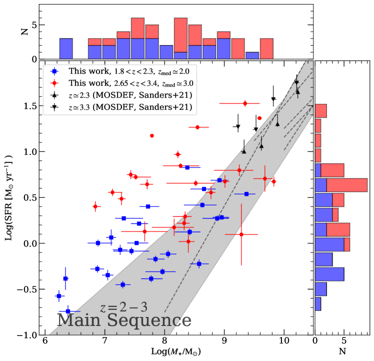
Figure 2: The distribution of galaxies in our sample on the SFR–$M_{\star}$ plane. The red squares show the $z\simeq 2$ sample and the red hexagons show the $z\simeq 3$ sample. The MOSDEF stacked results are denoted in black triangles. The gray shaded regions shows the (extrapolated) galaxy main sequence at $z=2-3$ based on the results from Speagle et al. (2014), Schreiber et al. (2015), Santini et al. (2017), Pearson et al. (2018), and Leja et al. (2022). The origin results from these works are denoted as gray dashed lines. The top and right panels show the stellar mass and SFR distributions respectively, with the $z\simeq 2$ sample in red and $z\simeq 3$ sample in blue.

Based on the spectral and photometric data, we measure and derive the galaxy properties from the emission line intensities and the SED fitting using multiple-band photometry. In this section, we present the methodology for the measurement and derivation of galaxy properties and show the results of MZR.

3.1 Emission-line Flux

To measure the intensity of galaxy emission lines, we use the Gaussian profile models to fit the lines in continuum-subtracted grism spectra. The line wavelengths are fixed by the galaxy’s redshift, which is determined by the SSP fitting as presented in Sec 2.1. For the H$\alpha$ and [O II] lines, we fit the spectra using a single 1D Gaussian function. For the H$\beta$+[O III]$\lambda\lambda 4959,5007$ lines, we fit the spectra using three Gaussian functions. We fix the line ratio of the [O III] doublet to [O III]$\lambda 4959$/[O III] $\lambda 5007=1/3$ and require the line width of [O III] doublet to be equal. We further verify the accuracy of our derived flux by comparing our measurements to the modeled flux solution fitted by Grizli and find the two to be consistent. A thorough summary of the best-fit observed emission line fluxes can be found in Appendix A.

In the early era of JWST observations, data calibration cannot be completely accurate (e.g., Rigby et al., 2022b). To minimize calibration issues, we employed reference calibration files that have been corrected using space-based observations. To quantify the effect of any remaining systematic errors on our data, we compared the NIRISS-extracted spectra with previous HST/WFC3 grism observations. We found that the estimated relative flux calibration error between different filter bands was limited to $\lesssim 5\%$, which is consistent with values reported in previous literature (e.g., Wang et al., 2022a).

3.2 Stellar Mass and Star Formation Rate

Galaxy stellar masses are derived by SED fitting to the photometry shown in Sec 2.2. Note that both A2744 and SMACS 0723 clusters significantly magnify the background sources, including galaxies in this work due to the gravitational lensing. In order to calculate the lensing magnification of each galaxy at the appropriate redshift, we adopt lensing models from Mahler et al. (2018) and Golubchik et al. (2022), respectively (see Appendix A). To do our analysis, we first correct the magnitudes in all bands by the lensing magnification factor. Note that we do not introduce the systematic error of lensing models. To simultaneously measure the stellar mass ($M_{\star}$), the stellar dust attenuation ($\rm E(B-V)_{star}$), and the best-fit model of the stellar continuum with emission lines, we fit the SED using the Bayesian code BEAGLE (Chevallard & Charlot, 2016). For our SED fitting, we fix the galaxy redshift, assume a constant star formation history, and model the dust attenuation curve following Calzetti et al. (2000). We set the dust attenuation in the $\mathrm{V}$ band $A_{\mathrm{V}}$ to vary from $0-8$ and use the Chabrier (2003) initial mass function (IMF) with an upper limit of $300~{}\mathrm{M}_{\odot}$. The metallicity of the interstellar medium (ISM) is assumed to be the same as that of the stellar populations. The nebular line and continuum emission are included in our fitting based on the CLOUDY photoionization code (Ferland et al., 2017). To model the metallicity, we use a flat prior with values ranging from $-2<\log(Z/\mathrm{Z}_{\odot})<0.4$. For our model, we bound the ionization parameter in log-space between $-4<\log U<-1$.

The derivation of star formation rate (SFR) and gaseous metallicity is based on the attenuation-corrected emission line intensities. We correct the reddening effect of dust attenuation for all measured nebular lines using the $\rm E(B-V)_{star}$ which is derived from the SED fitting, assuming the dust reddening for the nebular and stellar components are equal. Indeed, several works (e.g., Shivaei et al., 2020) pointed out that $\rm E(B-V)_{star}$ could equal to $\sim 2\rm E(B-V)_{gas}$ for galaxies at $z=2$, we test using this assumption and found out that the SFR could be increased by 0.1 dex. Furthermore, the relative changing line ratios (e.g., $\rm O_{32}$) are at an average level of 0.03 dex, which will lead to consistent conclusions in this paper. Therefore, in the rest of the paper, we adopt the assumption of $\rm E(B-V)_{star}=\rm E(B-V)_{gas}$.

Note that the nebular dust attenuation can be also derived from H$\alpha$/H$\beta$ Balmer decrement (e.g., H$\alpha$/H$\beta$ or H$\beta$/H$\gamma$) for a few galaxies in our sample. But half of our galaxy sample does not have H$\alpha$ coverage. The absence of H$\alpha$ line coverage and lack of significant H$\gamma$ line detection makes it impossible to measure dust attenuation via the Balmer decrement. To maintain consistency among our entire sample, we adopt the dust attenuation from the SED fitting to perform the de-reddening correction for emission lines.

We measure the SFR using the attenuation-corrected H$\alpha$ luminosity. For galaxies without H$\alpha$ coverage, we derive the H$\alpha$ luminosity from the attenuation-corrected H$\beta$ flux by adopting a Balmer decrement of H$\alpha$/H$\beta$=2.86. In order to estimate the SFR we assume the Kennicutt (1998) SFR calibration and the Chabrier (2003) initial mass function. The SFR is modeled as

$$\mathrm{SFR}=4.6\times 10^{-42}\frac{L_{\mathrm{H\alpha}}}{\rm erg~{}s^{-1}}[\mathrm{M}_{\odot}~{}\mathrm{yr}^{-1}],$$ (1)

where $L_{\mathrm{H\alpha}}$ is the H$\alpha$ luminosity. Throughout this paper, SFR corresponds to the $\rm SFR_{H\alpha}$, which is derived from the attenuation-corrected H$\alpha$ luminosity. And for those galaxies without H$\alpha$ coverage, we get H$\alpha$ luminosity using the attenuation-corrected H$\beta$ assuming a Balmer decrement of H$\alpha$/H$\beta$=2.86.

Within our sample, it is worth mentioning that the H$\alpha$ line is blended with [N II] lines due to the low spectral resolution, which biases our estimate of H$\alpha$ towards a higher value. However, the contribution of [N II] decreases with metallicity and typically the [N II]/H$\alpha$ is less than 0.07 for star-forming galaxies with the stellar mass of $M_{\star}<10^{9}\mathrm{M}_{\odot}$ at $z=2-3$ (e.g., Bian et al., 2018). Therefore, the [N II] contamination should be negligible to our SFR measurement, especially when compared with the uncertainty of dust attenuation correction. Besides, Balmer line stellar absorption can bias the intrinsic line luminosity to a lower value. Nevertheless, for the young star-forming galaxies in our sample, the Balmer line stellar absorption is comparatively weak and marginalized.

Using the measurements from SED fitting and SFR calibration, we plot Log(SFR) as a function of the Log(M_⋆), in Figure 2. We find that the relation between SFR and $M_{\star}$ displays a positive correlation across the complete range of stellar masses and redshift. We also find this slope agrees with the more massive galaxies measured in the MOSDEF sample Sanders et al. (2021) and the extrapolated galaxy star-forming main sequence. Despite a large degree of scatter, the SFR at fixed $M_{\star}$ increases with the redshift (Figure 2). However, when compared with previous studies of star-forming main sequence galaxies at redshifts of $2<z<3$, our sample of galaxies has a slightly higher mean SFR.

Table 1: Properties of stacked spectra in bins of $M_{\star}$ for the $z\simeq 2.0$ and $z\simeq 3.0$ samples.

log$(M_{\star}/\mathrm{M}_{\odot})$	N	($\rm 12+log(O/H)$)stack	($\rm 12+log(O/H)$)med	$\rm O_{32}$	$\rm O_{3}$	SFR [$\mathrm{M_{\odot}~{}yr^{-1}}$]
$1.8<z_{\mathrm{grism}}<2.3$
$6.64\pm{0.12}$	8	$8.03\pm{0.05}$	$8.00\pm{0.10}$	$0.86\pm{0.08}$	$0.59\pm{0.04}$	$0.61\pm{0.12}$
$7.56\pm{0.09}$	9	$8.11\pm{0.03}$	$8.05\pm{0.06}$	$0.73\pm{0.06}$	$0.79\pm{0.04}$	$1.09\pm{0.25}$
$8.50\pm{0.09}$	6	$8.23\pm{0.03}$	$8.26\pm{0.06}$	$0.52\pm{0.05}$	$0.74\pm{0.04}$	$2.61\pm{0.95}$
$9.25\pm{0.20}$	4	$8.35\pm{0.02}$	$8.38\pm{0.07}$	$0.32\pm{0.03}$	$0.55\pm{0.03}$	$2.83\pm{0.57}$
$2.65<z_{\mathrm{grism}}<3.4$
$7.48\pm{0.09}$	7	$8.00\pm{0.04}$	$7.98\pm{0.08}$	$0.91\pm{0.06}$	$0.75\pm{0.03}$	$5.02\pm{1.77}$
$8.39\pm{0.10}$	6	$8.14\pm{0.03}$	$8.10\pm{0.05}$	$0.67\pm{0.04}$	$0.78\pm{0.03}$	$5.60\pm{2.35}$
$9.62\pm{0.06}$	4	$8.34\pm{0.02}$	$8.40\pm{0.09}$	$0.34\pm{0.03}$	$1.01\pm{0.10}$	$10.64\pm{6.97}$

Note. — Column 1 is the median stellar mass for each bin; Column 2 is the number of galaxies in each bin; Columns 3 and 4 are gas phase metallicity measured from the stacked spectra and statistical median of individual galaxies, respectively; Column 5 and 6 are the line ratios O${}_{32}=$ log([O III]$\lambda\lambda 4959,5007$/[O II]$\lambda\lambda 3727,3729$) and $\mathrm{O}_{3}$=log([O III]$\lambda\lambda 4959,5007$/H$\beta$) derived from the stacked spectra; Column 7 is the median star formation rate.

3.3 Gas-phase Metallicity

Bian et al. (2018) established empirical relations between the strong metallicity diagnostic line ratios and the direct-$\mathrm{T_{e}}$ metallicity using a sample of local analogs of high-redshift galaxies. These calibrations have been demonstrated as one of the most reliable metallicity calibrations at $z>1$ (Sanders et al., 2020).

We derive the gas-phase oxygen abundance by adopting the Bian et al. (2018) calibration and measuring the strong metallicity diagnostic line ratios O${}_{32}=$ log([O III]$\lambda\lambda 4959,5007$/[O II]$\lambda\lambda 3727,3729$) and $\mathrm{O}_{3}$=log([O III]$\lambda\lambda 4959,5007$/H$\beta$). This calibration allows us to minimize the systematic uncertainty of the metallicity measurements when comparing our MZR results with those from Sanders et al. (2021). For the galaxies with both [O III] and [O II] coverage (44/51), we use the $\mathrm{O_{32}}$ to measure the gas-phase oxygen abundance as follows

$$12+\mathrm{log(O/H)}=8.54-0.59\times\mathrm{O_{32}}.$$ (2)

As shown above, we use the Bian et al. (2018) calibration, which is suitable in the range of $0.3<\mathrm{O_{32}}<1.2$ to measure the oxygen abundance in our galaxies. For the galaxies (11/48) where $\rm O_{32}$ is out of this range, we extrapolate this relation linearly to estimate their oxygen abundance. The linearity of the O₃₂ calibration allows us to extrapolate with minimal systematic error. For the same reason, we try not to use the $\rm R_{23}$ and $\rm O_{3}$ to further constrain the metallicity, which will cause more systematic uncertainties, especially for low-mass and low-metallicity galaxies.

For galaxies without [O II] coverage (7/51), we calculate the metallicity by using line ratio $\mathrm{O_{3}}\equiv$ [O III]$\lambda\lambda$4959,5007/H$\beta$, and use the following equation:

$$\mathrm{O_{3}}=43.9836-21.6211x+3.4277x^{2}-0.1747x^{3},$$ (3)

where $x=12+\mathrm{log(O/H)}$.

For the above $\mathrm{O_{3}}-Z$ relation, there exist two oxygen abundance solutions for a given $\mathrm{O_{3}}$ value. We adopt the solution within the range of $7.8<12+\log(\mathrm{O/H})<8.4$, which is consistent with the oxygen abundance range derived from $\mathrm{O_{32}}$ indicator in a similar mass range. Our derived metallicities are presented in Appendix A.

Additionally, we stack each individual spectrum to increase the signal-to-noise and measure the average metallicity in different stellar mass and redshift bins. We perform the spectrum stacking in two redshift bins ($1.8<z<2.3$ and $2.65<z<3.4$). For our stacking analysis, we only use the galaxies in the A2744 field, because those in the SMACS 0723 field do not have [O II] coverage. We divide the entire galaxy sample into four (three) stellar mass bins within the redshift range $1.8<z<2.3$ ($2.65<z<3.4$). Each stellar mass bin contains between four and nine galaxies, which is determined by the bootstrap simulation to minimize the uncertainty of derived metallicities of stacked spectra. Moreover, we ensure uniformity of the median stellar mass of each mass bin when setting the galaxy number in each bin.

For our stacking analysis, we first shift each spectrum into the rest frame according to the grism redshift. We then apply dust-corrections following the E(B-V) values from our SED fitting and the Calzetti et al. (2000) attenuation curve. We then subtract off the continuum for each individual spectrum before normalization and stacking. We normalized each spectrum based on their [O III] flux and resampled it onto a uniform wavelength grid. Lastly, the spectra in each mass bin are combined by taking the mean of the 3-$\sigma$ clipping of each wavelength grid. In Figure 1(b), we present the final stacked spectra in different stellar mass and redshift bins. We measure the relative emission line flux in the stacked spectra using the same method as for the individual galaxies. We derive gas-phase metallicities using the $\mathrm{O}_{32}$ indicator. The measurement uncertainties are propagated from both the stacking and line flux fitting. The median stellar mass, measured line ratios, median SFR, and the derived metallicity of stacked spectra are presented in Table 1.

It’s important to note that performing the dust correction either before or after stacking during the stacking procedure could potentially introduce bias to the measured metallicity(e.g., Henry et al., 2021). We performed a test by changing the sequence of dust corrections. Consequently, we find that the difference in derived metallicity 12+log(O/H) is 0.01 - 0.03 typically, which is within $1\sigma$ error of metallicity $\simeq 0.02-0.04$. Therefore, our results are not sensitive to the dust correction sequence when stacking. We also measure the dust attenuation using the Balmer decrement on the stacked spectra that are not dust-corrected.

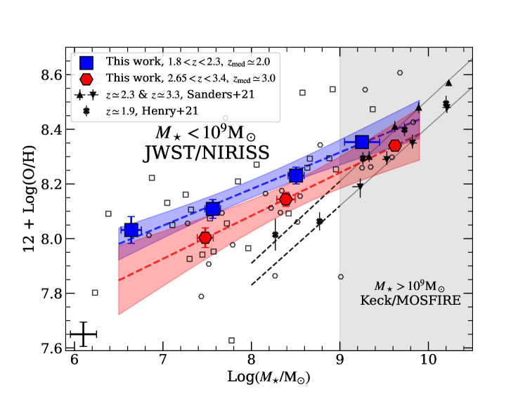
Figure 3: The mass-metallicity relation (MZR) for dwarf galaxies at $z\simeq 2$ (blue) and $z\simeq 3$ (red). The unfilled squares and hexagons denote individual galaxies at $z\simeq 2$ and $\simeq 3$ respectively. The large blue squares and red hexagons mark the results based on stacked spectra. The error bar in the lower left corner displays the median uncertainty of the individual galaxies. The best-fit results are denoted by the colored dashed lines, with their $1\sigma$ uncertainties in the shaded region.The MOSDEF stacked results (Sanders et al., 2021) are marked as black triangles and Henry et al. (2021) stacked results are marked as black crosses. The MOSDEF best-fit result and the extrapolation to the low-mass end are in solid and dashed lines.

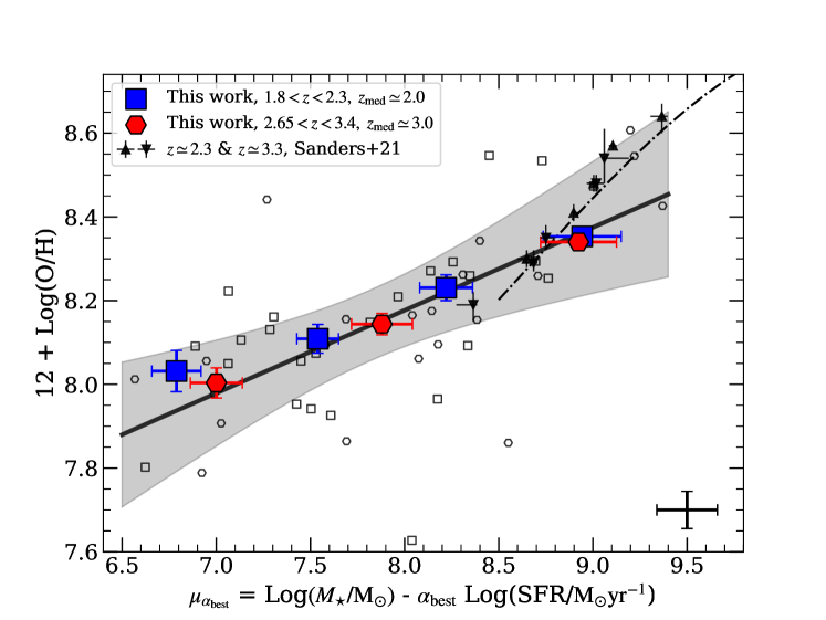
Figure 4: Projection of the fundamental metallicity relation (FMR) as O/H vs. $\mu_{\alpha_{\mathrm{best}}}=\operatorname{log}(M/\mathrm{M_{\odot}})-\alpha_{\mathrm{best}}\times\operatorname{log}(\mathrm{SFR/M_{\odot}~{}yr^{-1}})$. The coefficient $\alpha_{\mathrm{best}}=0.60$, minimizes the scatter of the O/H for our sample. The solid black line shows the best linear fit from Equation 4 and the grey-shaded region shows the $1\sigma$ uncertainty. The unfilled squares and hexagons represent individual galaxies at $z\simeq 2$ and $z\simeq 3$ respectively, and the large colored ones show the stacked results. The black triangles denote the MOSDEF stacked results from Sanders et al. (2021) and the black dotted-dashed line marks their best-fit. The error bar in the lower right corner displays the median uncertainty of the individual galaxies.

3.4 The Mass–Metallicity Relation

We find a clear correlation between gas-phase metallicity and stellar mass for our measurements of both individual galaxies and composite spectra. This is the first-ever effort to derive the MZR down to galaxies of $M_{\star}=10^{6.5}\mathrm{M}_{\odot}$ at $z=2-3$ using grism slitless spectroscopy. Within both the $z\simeq 2$ and $z\simeq 3$ sample, we find Spearman correlation coefficients of 0.70 and 0.68, respectively, with the statistical-significant p-value $<10^{-4}$. This means a positive correlation with strong evidence to reject the null hypothesis.

Beyond the strong trends of the MZR within each sample, we also look for signs of redshift evolution. Using the stacked spectra for the two samples, we find that the MZRs at $z\simeq 2.0$ and $z\simeq 3.0$ show a monotonic evolution toward lower metallicity with increasing redshift. As seen in Figure 3, the scale of this evolution is similar to that of MOSDEF from $z\simeq 2.3$ to $z\simeq 3.3$.

To quantify the MZR and derive slope and normalization, we fit it using a power law of the form:

$$\mathrm{12+log(O/H)}=\beta\times\mathrm{log}\left(\frac{M_{\star}}{10^{8}~{}\mathrm{M}_{\odot}}\right)+Z8,$$ (4)

where $Z8$ is the metallicity at the stellar mass of $10^{8}~{}\mathrm{M}_{\odot}$. Using all galaxies in the sample, we get the best-fit relations with $1\sigma$ uncertainties are:

$$\mathrm{12+log(O/H)} =$$ (5)

$$(0.14\pm 0.04)\times \mathrm{log}\left(\frac{M_{\star}}{10^{8}~{}\mathrm{M}_{\odot}}\right)+(8.14\pm 0.03).$$

We also fit the stacked spectra in the $z\simeq 2.0$ and $z\simeq 3.0$. The best-fit parameters with $1\sigma$ uncertainties are as follows: for $z\simeq 2.0$, $\beta_{z\simeq 2}=0.13\pm 0.04$, $Z8_{z\simeq 2}=8.18\pm 0.02$; and for $z\simeq 3.0$, $\beta_{z\simeq 3}=0.16\pm 0.03$, $Z8_{z\simeq 3}=8.08\pm 0.03$. These two best-fit relations and the M-Z values of each individual galaxy are shown in Figure 3.

Note that the slope of best-fit MZR for all stacked spectroscopy is $0.14\pm 0.04$, consistent with both $z\simeq 2$ and $z\simeq 3$ best-fit slopes, implying that there is no significant evolution in the slope between $z=2-3$. In contrast to the lack of evolution in the slope, we do find moderate evolution in the MZR normalization with redshift between $z=2-3$. Specifically, we find that the difference in the normalization at $z\simeq 2$ and $z\simeq 3$ is $\mathrm{\Delta log(O/H)}/\mathrm{\Delta}z=-0.09\pm 0.06$. Beyond redshift evolution, we also probe for differences in the MZR as a function of stellar mass. We find that at the low-mass end, we measure a much shallower slope than at the high-mass end mass where $\beta\simeq 0.30$ (Sanders et al., 2021). This suggests a transition in the slope of the MZR at $M_{\star}\simeq 10^{9}\mathrm{M}_{\odot}$.

Although our sample is not large enough to allow a statistically robust study of the scatter of the MZR at the low-mass end, we find a tentative increase of the MZR scatter at the stellar mass less than $10^{8}~{}\mathrm{M}_{\odot}$. By defining the intrinsic scatter as $\sigma_{\mathrm{ins}}=\sqrt{\sigma_{\mathrm{obs}}^{2}-\sigma_{\mathrm{meas}}^{2}}$, where $\sigma_{\mathrm{obs}}$ is the observation scatter and $\sigma_{\mathrm{meas}}$ is the measurement uncertainties, we measure the intrinsic scatter to be $0.16-0.18$ dex at $M_{\star}=10^{8}-10^{9}\mathrm{M}_{\odot}$. However, we see this value increase to $\approx 0.23$ dex at $M_{\star}=10^{7}\mathrm{M}_{\odot}$ bins implying a tentative evolution in the scatter.

4 Discussion

Using imaging from HST/ACS, HST/WFC3, JWST/NIRISS, and JWST/NIRCAM and grism spectroscopy from JWST/NIRISS, we present a study of the MZR in high-$z$ ($z=2-3$), low-mass galaxies ($10^{6.5}~{}\mathrm{M}_{\odot}<M_{\star}<10^{9.5}\mathrm{M}_{\odot}$), which probes approximately two orders of magnitude lower than previous studies. The best-fit slope of the MZR in dwarf galaxies at $z=2-3$ is $0.14\pm 0.04$, shallower than that of more massive galaxies ($M_{\star}>10^{9}\ \mathrm{M}_{\odot}$) at $z\approx 2-3$. Additionally, we measure moderate evolution in the MZR between the $z\simeq 2$ and $z\simeq 3$. The primary difference between our two redshift samples is the normalization, which differs by $\mathrm{\Delta log(O/H)}/\mathrm{\Delta}z=-0.09\pm 0.06$. In the following discussion, we provide a detailed physical interpretation of these results.

4.1 The MZR slope at low-mass end

Deep JWST/NIRISS spectroscopy of a sample of dwarf galaxies allows us, for the first time, to make a robust measurement of the slope of MZR at $z=2-3$ using low mass galaxies ($M_{\star}\approx 10^{6.5-9.5}\ \mathrm{M}_{\odot}$). At $z=2-3,$ we find a shallower slope in MZR at the low-mass end, in contrast to Sanders et al. (2021), which examines a sample of galaxies with $M_{\star}=10^{9}-10^{11}\mathrm{M}_{\odot}$. This difference indicates a transition in MZR slope around $M_{\star}\simeq 10^{9}\mathrm{M}_{\odot}$.

The differences in our measurements of the MZR slope may be indicative of differences in the feedback mechanisms that regulate it (e.g., Wang et al., 2022b; Strom et al., 2022). Typically, stellar feedback drives the gas and metal out of galaxies, which will result in differences in the gas-phase metallicity of the ISM. The feedback of stellar winds can be described by the wind mass loading factor ($\eta\equiv\dot{M}_{\mathrm{out}}/\mathrm{SFR}$), which presents the fraction of gas ejected in winds. The wind mass loading factor $\eta$ is related to the wind velocity ($v_{w}$), with $\eta\propto v_{w}^{-2}$ for the energy-driven wind model, $\eta\propto v_{w}^{-1}$ for the momentum-driven wind model, and $\eta\equiv\mathrm{const}$ for the constant wind model. We argue that the shallower MZR slope at the low-mass end is caused by that galaxies with different masses could be dominated by different feedback mechanisms.

For example, similar to our analysis, Torrey et al. (2019) used IllustrisTNG simulations and similarly found that the MZR has a shallower slope at the low-mass end. They argue that their results are indicative that feedback in low-mass galaxies may be dominated by constant wind ($\eta=\rm constant$), while feedback in high-mass galaxies may be dominated by energy-driven wind ($\eta\propto v_{w}^{2}$). Similarly, Pillepich et al. (2018) presents the necessity to introduce a constant wind model to match the low mass end of the galaxy stellar mass function. Specifically, the constant wind velocity reduces the wind mass loading factor. The larger-than-expected wind velocity and lower mass loading factor further result in longer wind recycling times and less direct metal ejection, which manifests as somewhat higher metallicities in the ISM and shallower MZR slope for low-mass galaxies, in agreement with our results.

Our best fit MZR slope is $\beta=0.14\pm 0.04$, which is consistent with the prediction of the momentum-driven wind model (e.g., Finlator & Davé, 2008; Guo et al., 2016). Such a slope suggests that momentum-driven wind is the dominant feedback in dwarf galaxies, in contrast to the constant wind models in Torrey et al. (2019). One possible interpretation is that the measured MZR slope in our sample is the average effect of a transition between the energy-driven wind model and constant wind models (the slope of the MZR in momentum-driven wind models is between the other two models). In this interpretation, the momentum-driven wind model ($\eta\propto v_{w}^{-1}$) acts as an intermediate state between the energy-driven wind ($\eta\propto v_{w}^{-2}$) and constant wind ($\eta\equiv\mathrm{const}$). Thus, a more general power-law wind model could be written as $\eta\propto v_{w}^{-\alpha_{\mathrm{fb}}}$ where $\alpha_{\mathrm{fb}}$ is the power index parameter of the feedback. Our results indicate that there could exist a continuous transition of wind model power index from $\alpha_{\mathrm{fb}}=2$ to $\alpha_{\mathrm{fb}}=0$ in low-mass galaxies with a transition stellar mass of $M_{\star}\simeq 10^{9}~{}\mathrm{M}_{\odot}$.

The slope of the MZR at the low-mass end remains not well constrained and is under debate. For example, Henry et al. (2021) found that the MZR slope for galaxies with stellar masses $M_{\star}>10^{8}~{}M_{\odot}$ at $z\simeq 1.9$ could remain steep, similar to that of higher-mass galaxies. However, the low-mass MZR slope we find is shallower. The discrepancy with Henry et al. (2021) could arise from several factors, including the different metallicity calibration methods used. As Sanders et al. (2020) suggested, we employ strong line calibration from Bian et al. (2018) and use $\rm O_{32}$ as the metallicity indicator. In contrast, Henry et al. (2021) derived metallicities based on Curti et al. (2017) using joint fitting of multiple line ratios. The choice of strong lines and calibration method could lead to a systematic discrepancy in MZR slope and normalization. To better compare our results with Henry et al. (2021), we recalculated the metallicities from their stacked measurements (overlaid in Figure 3), using our method based on the Bian et al. (2018) calibration. We find that the stacked results at $M_{\star}<10^{9}\mathrm{~{}M_{\odot}}$ show a tendency to follow the shallower-sloped MZR compared to the higher-mass points. To better constrain the validity of the slope transition hypothesis, we require further observations of the low-mass MZR and a more robust comparison to simulations.

4.2 The Evolution of MZR from z=3 to z=2

For fixed stellar mass $M_{\star}$, we find that the MZR normalization moderately evolves from lower O/H to higher O/H from $z=3$ to $z=2$. Moreover, we also aim to determine any evolution with stellar mass by comparing with Sanders et al. (2021). For the high-mass end ($M_{\star}\simeq 10^{10}\mathrm{~{}M_{\odot}}$), the normalization evolution is $\mathrm{\Delta log(O/H)}/\mathrm{\Delta}z=-0.11\pm 0.02$, while for the result in this work, we found $\mathrm{\Delta log(O/H)}/\mathrm{\Delta}z=-0.09\pm 0.06$ ($M_{\star}\simeq 10^{8}\mathrm{~{}M_{\odot}}$). It concludes that the evolution of the MZR is independent of galaxy stellar mass, as indicated by an unchanged MZR shape from $z=3$ to $z=2$ in a wide stellar mass range of $10^{6}-10^{10}~{}\mathrm{M}_{\odot}$.

The evolution of MZR is the consequence of a complicated interplay between star formation efficiency, galactic feedback, gas fraction, gas accretion, and recycling (e.g., Lilly et al., 2013). Thus, studies of MZR evolution can be used to constrain how the above processes evolve with cosmic time. Along these lines, Onodera et al. (2016) explain the evolution of the MZR normalization by suggesting that star-formation efficiency evolves weakly with redshift. However, Sanders et al. (2021) suggest an increasing star-formation efficiency with redshift to match their mild MZR evolution ($\mathrm{\Delta log(O/H)}/\mathrm{\Delta}z\simeq-0.1$). An increase in star-formation efficiency with redshift is consistent with recent studies on the evolution of star-formation efficiency (e.g., Liu et al., 2019). In this work, we also find a similar mild MZR evolution ($\mathrm{\Delta log(O/H)}/\mathrm{\Delta}z=-0.09\pm 0.06$) at the low-mass end, which suggests that star-formation efficiency increases with redshift across a wide stellar mass range.

The gas fraction of galaxies is another crucial factor for regulating the metallicity of galaxies. Observations have found that the gas fraction increases significantly with redshift at fixed $M_{\star}$ and has been quantified by $\mu_{\mathrm{gas}}\equiv M_{\mathrm{gas}}/M_{\star}\propto(1+z)^{2.5}$ (e.g., Tacconi et al., 2018). These large gas fractions can dilute the ISM of galaxies making lower gas-phase metallicity for higher redshift galaxies. Theoretically, the evolution of the gas fraction is considered the driving force of MZR evolution in some cosmological simulations (e.g., Ma et al., 2016; Torrey et al., 2019). However, the gas fraction is also predicted to increase with decreasing stellar mass at fixed redshift, which is quantified as $\mu_{\mathrm{gas}}\propto M_{\star}^{-0.4}$ for $z=2$ (e.g., Torrey et al., 2019). In contrast to previous studies, our results indicate that the evolution rate of MZR appears to be the same in the low-mass and high-mass end, implying that the high gas fraction of dwarf galaxies at $z=2-3$ may have a weak effect on the evolution of MZR. In the future, direct measurements of the gas fraction in dwarf galaxies (e.g., using the Square Kilometre Array, SKA) are crucial to understanding the effect and contribution of gas reservoirs on galaxy metal enrichment.

4.3 Existence of Fundamental Metallicity Relation in Dwarf Galaxies at $z=2-3$

Previous works (e.g., Ellison et al., 2008; Mannucci et al., 2010; Andrews & Martini, 2013) have suggested that a fundamental relation exists between metallicity and other galaxy properties. This fundamental metallicity relation (FMR), correlates the metallicity with both stellar mass and SFR. For a given stellar mass, the metallicity is enhanced with the decreasing SFR. Several works probing large samples of galaxies from $z=3$ to $z=0$ have found little redshift evolution in the FMR in galaxies above 10⁸  M_⊙ (e.g., Henry et al., 2013; Sanders et al., 2015, 2018; Curti et al., 2020; Henry et al., 2021). These results emphasize the dominance of stellar mass and SFR on the gas-phase metallicity of galaxies, regardless of the cosmic redshift.

The FMR relation can be explicitly parameterized using a two-dimensional projection with the relation between O/H and is written as

$$\mu_{\alpha}\equiv\operatorname{log}\left(\frac{M_{\star}}{\mathrm{M}_{\odot}}\right)-\alpha\times\operatorname{log}\left(\frac{\mathrm{SFR}}{\mathrm{M}_{\odot}~{}\mathrm{yr}^{-1}}\right).$$ (6)

In the above equation, $\alpha$ is introduced as the parameter to minimize the scatter in O/H. For the dwarf galaxies at $z=2-3$ in our sample, the scatter of O/H is minimized at $\alpha_{\mathrm{best}}=0.60\pm 0.13$, suggesting the existence of FMR for $z=2-3$ dwarf galaxies.

Based on our fitting, we construct an FMR with the linear function form of

$$\mathrm{12+log(O/H)}=(0.20\pm 0.02)\mu_{\alpha_{\mathrm{best}}}+(6.59\pm 0.15),$$ (7)

where $\mu_{\alpha_{\mathrm{best}}}=\operatorname{log}\left(M_{\star}/\mathrm{M}_{\odot}\right)-0.60\operatorname{log}\left(\mathrm{SFR}/{\mathrm{M}_{\odot}~{}\mathrm{yr}^{-1}}\right)$. We show the projection of the FMR, the O/H vs. $\mu_{\alpha_{\mathrm{best}}}$ in Figure 4. As seen in Figure 4, we find that the FMR exists within a large stellar mass range ($M_{\star}=10^{6}-10^{10}\mathrm{M}_{\odot}$) at $z=2-3$.

The existence of the FMR in the low stellar mass end demonstrates that the SFR and stellar mass act as the main physical properties for determining the gas-phase metallicity in dwarf galaxies at $z=2-3$. However, it is important to note that the exact measurement of parameter $\alpha$ and interpretation of the FMR can vary depending on the method used to measure it. For example, some works that have measured alpha for the FMR have found quite a range, with a systematic difference depending on whether the FMR was measured using a strong line calibration or direct metallicities in individual galaxies or stacks (e.g., Andrews & Martini, 2013; Henry et al., 2021). In the context of these studies, the results presented in this paper suggest that the FMR for dwarf galaxies at $z=2-3$ follows a consistent $\alpha$ value with previous measurements ($\alpha=0.55-0.7$; Andrews & Martini, 2013; Sanders et al., 2017, 2021; Curti et al., 2020). These measurements are over cosmic time ($z=0-3$), suggesting a slight evolution of FMR. However, we note that the slope of FMR in the low-mass end is much shallower than previous measurements, and further studies will be needed to fully understand the evolution of the FMR over cosmic time.

In the future, deeper imaging and spectroscopic observations over larger survey area will allow us to probe the MZR and FMR relations out to even higher redshifts and down to even lower metallicity. This will allow us to better understand the physical processes driving chemical enrichment at different epochs in the history of the Universe.

Appendix A Physical parameters for our sample

In Table A1, we show the measured and derived physical parameters of all of the galaxies in our sample, including galaxy ID defined by the Grizli spectrum extraction procedure, galaxy coordinates (R.A. and Decl.), galaxy redshift ($z_{\mathrm{grism}}$), stellar mass ($\mathrm{log}(M_{\star}/\mathrm{M}_{\odot})$), dust attenuation ($A_{V}$), star formation rate (SFR) derived from Balmer emission lines, line ratios ($\mathrm{O_{32}}=\operatorname{log}$([O III]/[O II])) and ($\mathrm{O_{3}}=\operatorname{log}$([O III]/H$\beta$)), and gas-phase “metallicity (12+log(O/H)). In Table A2, we present the observed line fluxes of [O II], H$\beta$, [O III], and H$\alpha$. Note that these fluxes have not been corrected by dust attenuation and gravitational lensing. The sample is divided into two redshift bins and presented for two fields A2744 and SMACS 0723.

Table A1: Measured and Derived Properties of Individual Galaxies

ID	R.A.	Decl.	$z_{\rm grism}$	log$(M_{\star}/\mathrm{M}_{\odot})$	$A_{V}$	SFR	$\mathrm{O}_{32}$	$\mathrm{O}_{3}$	$\rm 12+log(O/H)$	$\mu$
	deg.	deg.				$\rm M_{\odot}~{}yr^{-1}$
A2744 Field
$1.8<z_{\mathrm{grism}}<2.3$
34	3.591921	-30.415740	2.07	$7.72^{+0.19}_{-0.14}$	$0.33^{+0.05}_{-0.04}$	$2.82\pm{0.15}$	$0.87\pm{0.03}$	$0.85\pm{0.02}$	$8.03\pm{0.02}$	3.04
245	3.599965	-30.409570	1.81	$7.78^{+0.19}_{-0.17}$	$0.39^{+0.06}_{-0.08}$	$0.47\pm{0.05}$	$1.60\pm{0.89}$	$1.02\pm{0.11}$	$7.60\pm{0.52}$	6.29
282	3.577672	-30.408856	2.26	$7.05^{+0.09}_{-0.09}$	$0.01^{+0.01}_{-0.01}$	$0.45\pm{0.06}$	$0.69\pm{0.05}$	$0.48\pm{0.03}$	$8.13\pm{0.03}$	2.31
614	3.618857	-30.403802	2.20	$7.11^{+0.08}_{-0.08}$	$0.19^{+0.04}_{-0.04}$	$1.24\pm{0.25}$	$0.86\pm{0.13}$	$1.15\pm{0.28}$	$8.03\pm{0.08}$	1.00
882	3.602338	-30.400736	1.81	$8.58^{+0.16}_{-0.15}$	$0.20^{+0.08}_{-0.04}$	$0.64\pm{0.08}$	$0.04\pm{0.08}$	$0.63\pm{0.08}$	$8.52\pm{0.05}$	2.23
1018	3.606238	-30.397984	2.28	$6.89^{+0.24}_{-0.17}$	$0.12^{+0.05}_{-0.03}$	$1.05\pm{0.10}$	$1.68\pm{0.61}$	$0.80\pm{0.07}$	$7.55\pm{0.36}$	1.78
1085	3.604176	-30.397170	2.07	$9.37^{+0.15}_{-0.20}$	$0.38^{+0.05}_{-0.04}$	$3.93\pm{0.26}$	$0.16\pm{0.03}$	$0.75\pm{0.09}$	$8.44\pm{0.02}$	1.85
1333	3.606056	-30.393533	2.18	$8.42^{+0.18}_{-0.25}$	$0.30^{+0.09}_{-0.07}$	$1.48\pm{0.16}$	$0.80\pm{0.06}$	$1.13\pm{0.11}$	$8.07\pm{0.03}$	1.68
1407	3.611638	-30.392479	2.28	$7.45^{+0.30}_{-0.30}$	$0.13^{+0.04}_{-0.03}$	$0.86\pm{0.08}$	$1.03\pm{0.10}$	$1.05\pm{0.09}$	$7.93\pm{0.06}$	1.53
1409	3.599706	-30.392378	1.87	$7.85^{+0.15}_{-0.14}$	$0.15^{+0.04}_{-0.04}$	$0.71\pm{0.06}$	$0.58\pm{0.24}$	$0.63\pm{0.11}$	$8.20\pm{0.14}$	1.95
1445	3.607556	-30.391864	2.06	$6.34^{+0.06}_{-0.04}$	$0.16^{+0.06}_{-0.05}$	$0.44\pm{0.13}$	$1.85\pm{1.04}$	$0.87\pm{0.08}$	$7.45\pm{0.61}$	1.62
1461	3.604243	-30.391652	1.88	$8.06^{+0.14}_{-0.14}$	$0.29^{+0.06}_{-0.07}$	$0.85\pm{0.09}$	$0.50\pm{0.08}$	$0.92\pm{0.12}$	$8.25\pm{0.05}$	1.71
1500	3.607616	-30.391073	2.06	$7.26^{+0.12}_{-0.12}$	$0.47^{+0.06}_{-0.07}$	$1.00\pm{0.13}$	$0.71\pm{0.15}$	$0.95\pm{0.14}$	$8.12\pm{0.09}$	1.62
1503	3.603143	-30.391055	2.18	$7.57^{+0.15}_{-0.13}$	$0.13^{+0.03}_{-0.03}$	$1.72\pm{0.09}$	$1.01\pm{0.05}$	$0.87\pm{0.03}$	$7.94\pm{0.03}$	1.80
1504	3.613264	-30.391095	1.88	$8.66^{+0.19}_{-0.23}$	$0.42^{+0.06}_{-0.06}$	$4.50\pm{0.32}$	$0.48\pm{0.04}$	$0.87\pm{0.04}$	$8.26\pm{0.02}$	1.48
1573	3.609447	-30.389859	2.21	$8.96^{+0.12}_{-0.15}$	$0.25^{+0.05}_{-0.05}$	$2.09\pm{0.15}$	$0.52\pm{0.05}$	$0.66\pm{0.06}$	$8.23\pm{0.03}$	1.57
1596	3.610005	-30.389482	2.18	$8.63^{+0.24}_{-0.31}$	$0.32^{+0.07}_{-0.07}$	$2.92\pm{0.24}$	$0.52\pm{0.03}$	$0.90\pm{0.05}$	$8.23\pm{0.02}$	1.55
1685	3.603072	-30.387831	1.88	$6.23^{+0.10}_{-0.07}$	$0.28^{+0.10}_{-0.08}$	$0.29\pm{0.05}$	$1.29\pm{0.72}$	$1.07\pm{0.26}$	$7.78\pm{0.43}$	1.73
1823	3.579059	-30.385947	2.20	$7.53^{+0.19}_{-0.16}$	$0.14^{+0.03}_{-0.04}$	$1.06\pm{0.06}$	$0.81\pm{0.05}$	$0.82\pm{0.04}$	$8.06\pm{0.03}$	3.42
2032	3.592031	-30.382505	1.87	$6.87^{+0.11}_{-0.12}$	$0.16^{+0.04}_{-0.03}$	$0.56\pm{0.05}$	$0.56\pm{0.06}$	$0.77\pm{0.06}$	$8.21\pm{0.04}$	2.43
2084	3.591101	-30.381687	1.89	$8.38^{+0.22}_{-0.13}$	$0.27^{+0.02}_{-0.03}$	$7.38\pm{0.22}$	$0.70\pm{0.03}$	$1.00\pm{0.02}$	$8.13\pm{0.02}$	2.48
2152	3.585912	-30.380660	1.87	$7.32^{+0.32}_{-0.15}$	$0.29^{+0.03}_{-0.03}$	$2.07\pm{0.08}$	$0.77\pm{0.04}$	$0.86\pm{0.02}$	$8.08\pm{0.02}$	2.82
2186	3.610360	-30.380189	1.88	$8.92^{+0.15}_{-0.15}$	$0.48^{+0.05}_{-0.05}$	$5.72\pm{0.33}$	$0.05\pm{0.04}$	$0.63\pm{0.08}$	$8.51\pm{0.03}$	1.63
2303	3.607664	-30.378280	1.85	$6.38^{+0.21}_{-0.15}$	$0.07^{+0.04}_{-0.03}$	$0.19\pm{0.03}$	$0.77\pm{0.30}$	$0.43\pm{0.09}$	$8.09\pm{0.18}$	1.76
2313	3.598602	-30.378502	1.91	$8.88^{+0.20}_{-0.25}$	$0.27^{+0.07}_{-0.05}$	$2.05\pm{0.17}$	$0.45\pm{0.09}$	$0.88\pm{0.11}$	$8.27\pm{0.05}$	2.04
2330	3.599784	-30.377873	1.89	$7.96^{+0.22}_{-0.29}$	$0.10^{+0.07}_{-0.05}$	$0.51\pm{0.05}$	$0.99\pm{0.19}$	$0.74\pm{0.05}$	$7.96\pm{0.11}$	2.03
2421	3.599383	-30.375941	1.91	$7.30^{+0.13}_{-0.12}$	$0.06^{+0.02}_{-0.02}$	$0.36\pm{0.03}$	$1.05\pm{0.50}$	$0.63\pm{0.10}$	$7.92\pm{0.30}$	2.11
SMACS 0723 Field
$2.65<z_{\mathrm{grism}}<3.4$
50	110.821398	-73.474602	2.98	$8.78^{+0.07}_{-0.09}$	$0.38^{+0.02}_{-0.04}$	$8.66\pm{1.42}$	-	$0.73\pm{0.07}$	$8.35\pm{0.08}$	1.44
1347	110.823498	-73.444440	3.37	$8.22^{+0.06}_{-0.07}$	$0.17^{+0.02}_{-0.01}$	$14.00\pm{1.28}$	-	$0.89\pm{0.04}$	$8.12\pm{0.09}$	1.73
1361	110.859711	-73.444213	2.73	$9.01^{+0.08}_{-0.07}$	$0.12^{+0.03}_{-0.03}$	$6.27\pm{0.99}$	-	$0.97\pm{0.07}$	$7.87\pm{0.15}$	1.79
1424	110.828726	-73.442593	3.10	$9.59^{+0.04}_{-0.04}$	$0.31^{+0.01}_{-0.01}$	$47.29\pm{1.63}$	-	$0.77\pm{0.01}$	$8.30\pm{0.02}$	1.63
1475	110.863244	-73.441489	2.73	$8.33^{+0.09}_{-0.12}$	$0.24^{+0.04}_{-0.07}$	$2.90\pm{0.51}$	-	$0.90\pm{0.07}$	$8.10\pm{0.16}$	1.75
1491	110.859274	-73.441230	2.73	$9.83^{+0.02}_{-0.05}$	$0.30^{+0.04}_{-0.02}$	$9.45\pm{1.18}$	-	$0.65\pm{0.05}$	$8.43\pm{0.05}$	1.94
1520	110.850517	-73.440461	3.04	$7.71^{+0.10}_{-0.12}$	$0.18^{+0.07}_{-0.05}$	$6.77\pm{0.90}$	-	$0.63\pm{0.05}$	$8.44\pm{0.04}$	1.69

Note. — To be continued.

Table A1: (Continued)

ID	R.A.	Decl.	$z_{\rm grism}$	log$(M_{\star}/\mathrm{M}_{\odot})$	$A_{V}$	SFR	$\mathrm{O}_{32}$	$\mathrm{O}_{3}$	$\rm 12+log(O/H)$	$\mu$
	deg.	deg.				$\rm\mathrm{M}_{\odot}~{}yr^{-1}$
A2744 Field
$2.65<z_{\mathrm{grism}}<3.4$
404	3.613460	-30.406860	2.85	$6.84^{+0.09}_{-0.05}$	$0.06^{+0.03}_{-0.04}$	$2.56\pm{0.35}$	$0.90\pm{0.08}$	$0.69\pm{0.06}$	$8.01\pm{0.05}$	1.69
434	3.607437	-30.406471	3.20	$9.25^{+0.24}_{-0.42}$	$0.35^{+0.05}_{-0.09}$	$6.79\pm{1.03}$	$0.52\pm{0.04}$	$0.80\pm{0.05}$	$8.23\pm{0.02}$	2.18
538	3.612998	-30.405067	3.04	$9.35^{+0.24}_{-0.43}$	$0.43^{+0.04}_{-0.09}$	$36.97\pm{3.36}$	$0.53\pm{0.03}$	$0.46\pm{0.02}$	$8.23\pm{0.01}$	1.69
903	3.609749	-30.400342	2.97	$9.68^{+0.13}_{-0.19}$	$0.41^{+0.06}_{-0.04}$	$5.58\pm{1.85}$	$-0.06\pm{0.04}$	$0.77\pm{0.14}$	$8.57\pm{0.02}$	1.73
988	3.613656	-30.398646	2.85	$9.29^{+0.28}_{-0.27}$	$0.21^{+0.09}_{-0.04}$	$1.31\pm{1.02}$	$0.02\pm{0.07}$	$0.87\pm{0.34}$	$8.53\pm{0.04}$	1.56
1016	3.607800	-30.398054	3.20	$7.28^{+0.07}_{-0.06}$	$0.06^{+0.02}_{-0.02}$	$3.10\pm{0.50}$	$0.83\pm{0.05}$	$0.97\pm{0.07}$	$8.05\pm{0.03}$	1.77
1042	3.610340	-30.397893	3.36	$7.79^{+0.03}_{-0.03}$	$0.02^{+0.01}_{-0.01}$	$14.97\pm{0.55}$	$0.96\pm{0.02}$	$0.82\pm{0.02}$	$7.98\pm{0.01}$	1.67
1206	3.607114	-30.395622	2.98	$8.27^{+0.31}_{-0.29}$	$0.15^{+0.03}_{-0.03}$	$7.25\pm{0.46}$	$1.17\pm{0.05}$	$0.85\pm{0.02}$	$7.85\pm{0.03}$	1.72
1275	3.572769	-30.394578	2.94	$8.16^{+0.33}_{-0.37}$	$0.24^{+0.04}_{-0.05}$	$1.58\pm{0.35}$	$0.67\pm{0.06}$	$0.84\pm{0.09}$	$8.15\pm{0.03}$	3.25
1394	3.611255	-30.392440	2.98	$7.13^{+0.16}_{-0.07}$	$0.11^{+0.03}_{-0.03}$	$3.69\pm{0.35}$	$1.71\pm{0.62}$	$0.44\pm{0.04}$	$7.53\pm{0.37}$	1.57
1535	3.604198	-30.390338	2.71	$8.40^{+0.10}_{-0.16}$	$0.09^{+0.06}_{-0.04}$	$1.07\pm{0.30}$	$0.67\pm{0.16}$	$0.49\pm{0.13}$	$8.15\pm{0.10}$	1.79
1692	3.604118	-30.387855	2.84	$7.52^{+0.25}_{-0.07}$	$0.11^{+0.02}_{-0.02}$	$5.42\pm{0.35}$	$1.09\pm{0.04}$	$0.92\pm{0.03}$	$7.90\pm{0.02}$	1.76
2029	3.596739	-30.382570	3.21	$7.43^{+0.08}_{-0.06}$	$0.20^{+0.03}_{-0.03}$	$5.89\pm{0.66}$	$1.30\pm{0.09}$	$0.85\pm{0.05}$	$7.77\pm{0.06}$	2.16
2060	3.585941	-30.382101	3.06	$8.52^{+0.32}_{-0.49}$	$0.17^{+0.04}_{-0.04}$	$4.72\pm{0.35}$	$0.83\pm{0.02}$	$0.90\pm{0.03}$	$8.05\pm{0.01}$	3.33
2225	3.591399	-30.379771	2.73	$8.55^{+0.19}_{-0.15}$	$0.70^{+0.04}_{-0.05}$	$21.43\pm{1.34}$	$0.75\pm{0.01}$	$0.91\pm{0.01}$	$8.10\pm{0.01}$	2.50
2237	3.604111	-30.379262	2.83	$7.67^{+0.38}_{-0.39}$	$0.22^{+0.06}_{-0.06}$	$1.42\pm{0.36}$	$0.79\pm{0.11}$	$0.78\pm{0.11}$	$8.08\pm{0.07}$	1.95
2287	3.607475	-30.378498	2.69	$8.34^{+0.11}_{-0.20}$	$0.06^{+0.04}_{-0.03}$	$1.99\pm{0.25}$	$0.63\pm{0.08}$	$0.46\pm{0.06}$	$8.17\pm{0.05}$	1.83

Note. — Column 1 is the source ID defined by our source detection procedure; Columns 2 and 3 are the equatorial coordinates right ascension (R.A.) and declination (Decl.) in equinox with an epoch of J2000; Column 4 is the redshift determined by NIRISS grism spectra; Column 5 is the stellar mass; Column 6 is the dust attenuation ($A_{V}$); Column 7 is the star formation rate derived from Balmer emission lines; Columns 8 and 9 are the line ratios O${}_{32}=$ log([O III]$\lambda\lambda 4959,5007$/[O II]$\lambda\lambda 3727,3729$) and $\mathrm{O}_{3}$=log([O III]$\lambda\lambda 4959,5007$/H$\beta$); Column 10 is gas phase metallicity represented by oxygen abundance; Column 11 is the magnification of gravitational lensing effect.

Table A2: Measured emission line fluxes of Individual Galaxies

ID	$f_{\rm[OII]}$	$f_{\rm H\beta}$	$f_{\rm[OIII]}$	$f_{\rm H\alpha}$
	$10^{-17}~{}\rm erg~{}s^{-1}~{}cm^{-2}$	$10^{-17}~{}\rm erg~{}s^{-1}~{}cm^{-2}$	$10^{-17}~{}\rm erg~{}s^{-1}~{}cm^{-2}$	$10^{-17}~{}\rm erg~{}s^{-1}~{}cm^{-2}$
A2744 Field
$1.8<z_{\mathrm{grism}}<2.3$
34	$1.47\pm{0.10}$	$1.54\pm{0.07}$	$10.82\pm{0.10}$	$4.12\pm{0.11}$
245	$0.08\pm{0.17}$	$0.32\pm{0.08}$	$3.32\pm{0.09}$	$1.84\pm{0.12}$
282	$0.42\pm{0.05}$	$0.68\pm{0.04}$	$2.06\pm{0.06}$	$0.58\pm{0.08}$
614	$0.23\pm{0.07}$	$0.12\pm{0.07}$	$1.64\pm{0.09}$	$0.60\pm{0.12}$
882	$2.64\pm{0.45}$	$0.68\pm{0.12}$	$2.88\pm{0.12}$	$1.10\pm{0.11}$
1018	$0.04\pm{0.05}$	$0.29\pm{0.05}$	$1.85\pm{0.06}$	$0.89\pm{0.07}$
1085	$2.42\pm{0.15}$	$0.63\pm{0.13}$	$3.53\pm{0.15}$	$3.29\pm{0.13}$
1333	$0.49\pm{0.06}$	$0.23\pm{0.06}$	$3.10\pm{0.07}$	$1.09\pm{0.06}$
1407	$0.23\pm{0.05}$	$0.22\pm{0.05}$	$2.51\pm{0.06}$	$0.62\pm{0.05}$
1409	$0.36\pm{0.20}$	$0.32\pm{0.08}$	$1.38\pm{0.08}$	$1.05\pm{0.08}$
1445	$0.02\pm{0.05}$	$0.19\pm{0.04}$	$1.43\pm{0.05}$	$0.41\pm{0.12}$
1461	$0.53\pm{0.09}$	$0.20\pm{0.05}$	$1.65\pm{0.07}$	$0.92\pm{0.08}$
1500	$0.29\pm{0.10}$	$0.17\pm{0.05}$	$1.47\pm{0.07}$	$0.67\pm{0.08}$
1503	$0.49\pm{0.05}$	$0.68\pm{0.05}$	$5.00\pm{0.07}$	$1.63\pm{0.06}$
1504	$1.68\pm{0.14}$	$0.68\pm{0.06}$	$5.04\pm{0.08}$	$3.69\pm{0.07}$
1573	$0.68\pm{0.08}$	$0.49\pm{0.07}$	$2.25\pm{0.08}$	$1.47\pm{0.07}$
1596	$1.25\pm{0.07}$	$0.53\pm{0.06}$	$4.13\pm{0.09}$	$1.95\pm{0.07}$
1685	$0.04\pm{0.06}$	$0.06\pm{0.04}$	$0.73\pm{0.05}$	$0.33\pm{0.04}$
1823	$0.75\pm{0.08}$	$0.74\pm{0.07}$	$4.82\pm{0.09}$	$1.86\pm{0.08}$
2032	$0.69\pm{0.10}$	$0.42\pm{0.05}$	$2.50\pm{0.07}$	$1.01\pm{0.09}$
2084	$5.90\pm{0.43}$	$2.93\pm{0.14}$	$29.62\pm{0.17}$	$11.71\pm{0.14}$
2152	$1.85\pm{0.16}$	$1.51\pm{0.06}$	$11.00\pm{0.10}$	$3.77\pm{0.08}$
2186	$3.21\pm{0.29}$	$0.85\pm{0.15}$	$3.63\pm{0.17}$	$4.86\pm{0.14}$
2303	$0.11\pm{0.08}$	$0.24\pm{0.04}$	$0.65\pm{0.05}$	$0.27\pm{0.04}$
2313	$1.51\pm{0.31}$	$0.57\pm{0.14}$	$4.29\pm{0.16}$	$2.61\pm{0.14}$
2330	$0.22\pm{0.10}$	$0.39\pm{0.05}$	$2.13\pm{0.06}$	$0.80\pm{0.05}$
2421	$0.10\pm{0.11}$	$0.26\pm{0.06}$	$1.10\pm{0.07}$	$0.60\pm{0.05}$
SMACS 0723 Field
$2.65<z_{\mathrm{grism}}<3.4$
50	-	$0.77\pm{0.12}$	$4.12\pm{0.18}$	-
1347	-	$1.43\pm{0.13}$	$11.19\pm{0.20}$	-
1361	-	$1.18\pm{0.18}$	$11.05\pm{0.21}$	-
1424	-	$4.72\pm{0.14}$	$27.79\pm{0.21}$	-
1475	-	$0.46\pm{0.08}$	$3.65\pm{0.11}$	-
1491	-	$1.54\pm{0.18}$	$6.86\pm{0.22}$	-
1520	-	$0.86\pm{0.09}$	$3.68\pm{0.13}$	-

Note. — To be continued.

Table A2: (Continued)

ID	$f_{\rm[OII]}$	$f_{\rm H\beta}$	$f_{\rm[OIII]}$	$f_{\rm H\alpha}$
	$10^{-17}~{}\rm erg~{}s^{-1}~{}cm^{-2}$	$10^{-17}~{}\rm erg~{}s^{-1}~{}cm^{-2}$	$10^{-17}~{}\rm erg~{}s^{-1}~{}cm^{-2}$	$10^{-17}~{}\rm erg~{}s^{-1}~{}cm^{-2}$
A2744 Field
$2.65<z_{\mathrm{grism}}<3.4$
404	$0.27\pm{0.05}$	$0.44\pm{0.06}$	$2.18\pm{0.08}$	-
434	$1.51\pm{0.13}$	$0.80\pm{0.10}$	$5.03\pm{0.11}$	-
538	$2.91\pm{0.16}$	$3.44\pm{0.14}$	$9.83\pm{0.18}$	-
903	$3.89\pm{0.29}$	$0.58\pm{0.19}$	$3.41\pm{0.20}$	-
988	$1.22\pm{0.14}$	$0.17\pm{0.13}$	$1.28\pm{0.13}$	-
1016	$0.59\pm{0.06}$	$0.43\pm{0.07}$	$3.97\pm{0.08}$	-
1042	$1.34\pm{0.06}$	$1.82\pm{0.07}$	$12.14\pm{0.11}$	-
1206	$0.49\pm{0.05}$	$1.03\pm{0.05}$	$7.24\pm{0.08}$	-
1275	$0.58\pm{0.07}$	$0.39\pm{0.08}$	$2.68\pm{0.11}$	-
1394	$0.03\pm{0.04}$	$0.50\pm{0.04}$	$1.38\pm{0.06}$	-
1535	$0.14\pm{0.05}$	$0.21\pm{0.06}$	$0.65\pm{0.07}$	-
1692	$0.62\pm{0.06}$	$0.93\pm{0.05}$	$7.65\pm{0.08}$	-
2029	$0.29\pm{0.06}$	$0.82\pm{0.09}$	$5.80\pm{0.10}$	-
2060	$1.37\pm{0.07}$	$1.19\pm{0.07}$	$9.38\pm{0.10}$	-
2225	$3.97\pm{0.08}$	$2.74\pm{0.08}$	$22.15\pm{0.13}$	-
2237	$0.23\pm{0.06}$	$0.24\pm{0.06}$	$1.42\pm{0.07}$	-
2287	$0.30\pm{0.05}$	$0.43\pm{0.05}$	$1.25\pm{0.06}$	-

Note. — Column 1 is the source ID defined by our source detection procedure; Columns 2-5 present the observed emission line fluxes of [O II], H$\beta$, [O III], and H$\alpha$. Note that the “-” value means that the grism observations do not cover the corresponding wavelength.

References

- Andrews & Martini (2013) Andrews, B. H., & Martini, P. 2013, ApJ, 765, 140, doi: 10.1088/0004-637X/765/2/140
- Astropy Collaboration et al. (2022) Astropy Collaboration, Price-Whelan, A. M., Lim, P. L., et al. 2022, ApJ, 935, 167, doi: 10.3847/1538-4357/ac7c74
- Bergamini et al. (2022) Bergamini, P., Acebron, A., Grillo, C., et al. 2022, arXiv e-prints, arXiv:2207.09416. https://arxiv.org/abs/2207.09416
- Bertin & Arnouts (1996) Bertin, E., & Arnouts, S. 1996, A&AS, 117, 393, doi: 10.1051/aas:1996164
- Bian et al. (2018) Bian, F., Kewley, L. J., & Dopita, M. A. 2018, ApJ, 859, 175, doi: 10.3847/1538-4357/aabd74
- Boyett et al. (2022) Boyett, K., Mascia, S., Pentericci, L., et al. 2022, arXiv, arXiv:2207.13459. https://arxiv.org/abs/2207.13459
- Brammer et al. (2022) Brammer, G., Strait, V., Matharu, J., & Momcheva, I. 2022, grizli, 1.5.0, Zenodo, Zenodo, doi: 10.5281/zenodo.6672538
- Calzetti et al. (2000) Calzetti, D., Armus, L., Bohlin, R. C., et al. 2000, ApJ, 533, 682, doi: 10.1086/308692
- Chabrier (2003) Chabrier, G. 2003, PASP, 115, 763, doi: 10.1086/376392
- Chevallard & Charlot (2016) Chevallard, J., & Charlot, S. 2016, MNRAS, 462, 1415, doi: 10.1093/mnras/stw1756
- Coe et al. (2019) Coe, D., Salmon, B., Bradač, M., et al. 2019, ApJ, 884, 85, doi: 10.3847/1538-4357/ab412b
- Coil et al. (2015) Coil, A. L., Aird, J., Reddy, N., et al. 2015, ApJ, 801, 35, doi: 10.1088/0004-637X/801/1/35
- Curti et al. (2017) Curti, M., Cresci, G., Mannucci, F., et al. 2017, MNRAS, 465, 1384, doi: 10.1093/mnras/stw2766
- Curti et al. (2020) Curti, M., Maiolino, R., Cirasuolo, M., et al. 2020, MNRAS, 492, 821, doi: 10.1093/mnras/stz3379
- Eddington (1913) Eddington, A. S. 1913, MNRAS, 73, 359, doi: 10.1093/mnras/73.5.359
- Ellison et al. (2008) Ellison, S. L., Patton, D. R., Simard, L., & McConnachie, A. W. 2008, ApJL, 672, L107, doi: 10.1086/527296
- Erb et al. (2006) Erb, D. K., Shapley, A. E., Pettini, M., et al. 2006, ApJ, 644, 813, doi: 10.1086/503623
- Ferland et al. (2017) Ferland, G. J., Chatzikos, M., Guzmán, F., et al. 2017, RMxAA, 53, 385. https://arxiv.org/abs/1705.10877
- Finlator & Davé (2008) Finlator, K., & Davé, R. 2008, MNRAS, 385, 2181, doi: 10.1111/j.1365-2966.2008.12991.x
- Flewelling et al. (2020) Flewelling, H. A., Magnier, E. A., Chambers, K. C., et al. 2020, ApJS, 251, 7, doi: 10.3847/1538-4365/abb82d
- Gaia Collaboration et al. (2018) Gaia Collaboration, Brown, A. G. A., Vallenari, A., et al. 2018, A&A, 616, A1, doi: 10.1051/0004-6361/201833051
- Golubchik et al. (2022) Golubchik, M., Furtak, L. J., Meena, A. K., & Zitrin, A. 2022, ApJ, 938, 14, doi: 10.3847/1538-4357/ac8ff1
- Guo et al. (2016) Guo, Y., Koo, D. C., Lu, Y., et al. 2016, ApJ, 822, 103, doi: 10.3847/0004-637X/822/2/103
- Henry et al. (2013) Henry, A., Scarlata, C., Domínguez, A., et al. 2013, ApJL, 776, L27, doi: 10.1088/2041-8205/776/2/L27
- Henry et al. (2021) Henry, A., Rafelski, M., Sunnquist, B., et al. 2021, ApJ, 919, 143, doi: 10.3847/1538-4357/ac1105
- Juneau et al. (2011) Juneau, S., Dickinson, M., Alexander, D. M., & Salim, S. 2011, ApJ, 736, 104, doi: 10.1088/0004-637X/736/2/104
- Kennicutt (1998) Kennicutt, Robert C., J. 1998, ApJ, 498, 541, doi: 10.1086/305588
- Leja et al. (2022) Leja, J., Speagle, J. S., Ting, Y.-S., et al. 2022, ApJ, 936, 165, doi: 10.3847/1538-4357/ac887d
- Li et al. (2022) Li, Z., Wang, X., Cai, Z., et al. 2022, ApJL, 929, L8, doi: 10.3847/2041-8213/ac626f
- Lilly et al. (2013) Lilly, S. J., Carollo, C. M., Pipino, A., Renzini, A., & Peng, Y. 2013, ApJ, 772, 119, doi: 10.1088/0004-637X/772/2/119
- Lin et al. (2022) Lin, X., Cai, Z., Zou, S., et al. 2022, arXiv, arXiv:2209.03376. https://arxiv.org/abs/2209.03376
- Liu et al. (2019) Liu, D., Schinnerer, E., Groves, B., et al. 2019, ApJ, 887, 235, doi: 10.3847/1538-4357/ab578d
- Lotz et al. (2017) Lotz, J. M., Koekemoer, A., Coe, D., et al. 2017, ApJ, 837, 97, doi: 10.3847/1538-4357/837/1/97
- Ma et al. (2016) Ma, X., Hopkins, P. F., Faucher-Giguère, C.-A., et al. 2016, MNRAS, 456, 2140, doi: 10.1093/mnras/stv2659
- Mahler et al. (2018) Mahler, G., Richard, J., Clément, B., et al. 2018, MNRAS, 473, 663, doi: 10.1093/mnras/stx1971
- Maier et al. (2014) Maier, C., Lilly, S. J., Ziegler, B. L., et al. 2014, ApJ, 792, 3, doi: 10.1088/0004-637X/792/1/3
- Mannucci et al. (2010) Mannucci, F., Cresci, G., Maiolino, R., Marconi, A., & Gnerucci, A. 2010, MNRAS, 408, 2115, doi: 10.1111/j.1365-2966.2010.17291.x
- Nedkova et al. (2021) Nedkova, K. V., Häußler, B., Marchesini, D., et al. 2021, MNRAS, 506, 928, doi: 10.1093/mnras/stab1744
- Oke & Gunn (1983) Oke, J. B., & Gunn, J. E. 1983, ApJ, 266, 713, doi: 10.1086/160817
- Onodera et al. (2016) Onodera, M., Carollo, C. M., Lilly, S., et al. 2016, ApJ, 822, 42, doi: 10.3847/0004-637X/822/1/42
- Papovich et al. (2022) Papovich, C., Simons, R. C., Estrada-Carpenter, V., et al. 2022, ApJ, 937, 22, doi: 10.3847/1538-4357/ac8058
- Pearson et al. (2018) Pearson, W. J., Wang, L., Hurley, P. D., et al. 2018, A&A, 615, A146, doi: 10.1051/0004-6361/201832821
- Peeples & Shankar (2011) Peeples, M. S., & Shankar, F. 2011, MNRAS, 417, 2962, doi: 10.1111/j.1365-2966.2011.19456.x
- Pillepich et al. (2018) Pillepich, A., Nelson, D., Hernquist, L., et al. 2018, MNRAS, 475, 648, doi: 10.1093/mnras/stx3112
- Pontoppidan et al. (2022) Pontoppidan, K., Blome, C., Braun, H., et al. 2022, arXiv, arXiv:2207.13067. https://arxiv.org/abs/2207.13067
- Rigby et al. (2022a) Rigby, J., Perrin, M., McElwain, M., et al. 2022a, arXiv e-prints, arXiv:2207.05632. https://arxiv.org/abs/2207.05632
- Rigby et al. (2022b) —. 2022b, arXiv, arXiv:2207.05632, doi: 10.48550/arXiv.2207.05632
- Robertson et al. (2010) Robertson, B. E., Ellis, R. S., Dunlop, J. S., McLure, R. J., & Stark, D. P. 2010, Natur, 468, 49, doi: 10.1038/nature09527
- Sanders et al. (2017) Sanders, R. L., Shapley, A. E., Zhang, K., & Yan, R. 2017, ApJ, 850, 136, doi: 10.3847/1538-4357/aa93e4
- Sanders et al. (2015) Sanders, R. L., Shapley, A. E., Kriek, M., et al. 2015, ApJ, 799, 138, doi: 10.1088/0004-637X/799/2/138
- Sanders et al. (2018) —. 2018, ApJ, 858, 99, doi: 10.3847/1538-4357/aabcbd
- Sanders et al. (2020) Sanders, R. L., Shapley, A. E., Reddy, N. A., et al. 2020, MNRAS, 491, 1427, doi: 10.1093/mnras/stz3032
- Sanders et al. (2021) Sanders, R. L., Shapley, A. E., Jones, T., et al. 2021, ApJ, 914, 19, doi: 10.3847/1538-4357/abf4c1
- Santini et al. (2017) Santini, P., Fontana, A., Castellano, M., et al. 2017, ApJ, 847, 76, doi: 10.3847/1538-4357/aa8874
- Schlawin et al. (2020) Schlawin, E., Leisenring, J., Misselt, K., et al. 2020, AJ, 160, 231, doi: 10.3847/1538-3881/abb811
- Schreiber et al. (2015) Schreiber, C., Pannella, M., Elbaz, D., et al. 2015, A&A, 575, A74, doi: 10.1051/0004-6361/201425017
- Shipley et al. (2018) Shipley, H. V., Lange-Vagle, D., Marchesini, D., et al. 2018, ApJS, 235, 14, doi: 10.3847/1538-4365/aaacce
- Shivaei et al. (2020) Shivaei, I., Reddy, N., Rieke, G., et al. 2020, ApJ, 899, 117, doi: 10.3847/1538-4357/aba35e
- Speagle et al. (2014) Speagle, J. S., Steinhardt, C. L., Capak, P. L., & Silverman, J. D. 2014, ApJS, 214, 15, doi: 10.1088/0067-0049/214/2/15
- Steidel et al. (2014) Steidel, C. C., Rudie, G. C., Strom, A. L., et al. 2014, ApJ, 795, 165, doi: 10.1088/0004-637X/795/2/165
- Strom et al. (2022) Strom, A. L., Rudie, G. C., Steidel, C. C., & Trainor, R. F. 2022, ApJ, 925, 116, doi: 10.3847/1538-4357/ac38a3
- Tacconi et al. (2018) Tacconi, L. J., Genzel, R., Saintonge, A., et al. 2018, ApJ, 853, 179, doi: 10.3847/1538-4357/aaa4b4
- Torrey et al. (2019) Torrey, P., Vogelsberger, M., Marinacci, F., et al. 2019, MNRAS, 484, 5587, doi: 10.1093/mnras/stz243
- Tremonti et al. (2004) Tremonti, C. A., Heckman, T. M., Kauffmann, G., et al. 2004, ApJ, 613, 898, doi: 10.1086/423264
- Treu et al. (2022) Treu, T., Roberts-Borsani, G., Bradac, M., et al. 2022, ApJ, 935, 110, doi: 10.3847/1538-4357/ac8158
- Wang et al. (2020) Wang, X., Jones, T. A., Treu, T., et al. 2020, ApJ, 900, 183, doi: 10.3847/1538-4357/abacce
- Wang et al. (2022a) Wang, X., Jones, T., Vulcani, B., et al. 2022a, ApJL, 938, L16, doi: 10.3847/2041-8213/ac959e
- Wang et al. (2022b) Wang, X., Li, Z., Cai, Z., et al. 2022b, ApJ, 926, 70, doi: 10.3847/1538-4357/ac3974
- Wu et al. (2021) Wu, Y., Cai, Z., Neeleman, M., et al. 2021, Nature Astronomy, 5, 1110, doi: 10.1038/s41550-021-01471-4
- Wu et al. (2022) Wu, Y., Cai, Z., Sun, F., et al. 2022, arXiv, arXiv:2208.08473. https://arxiv.org/abs/2208.08473
- Zahid et al. (2012) Zahid, H. J., Bresolin, F., Kewley, L. J., Coil, A. L., & Davé, R. 2012, ApJ, 750, 120, doi: 10.1088/0004-637X/750/2/120
- Zahid et al. (2014) Zahid, H. J., Dima, G. I., Kudritzki, R.-P., et al. 2014, ApJ, 791, 130, doi: 10.1088/0004-637X/791/2/130