A New Test for Market Efficiency
and Uncovered Interest Parity

Abstract: We suggest a new single-equation test for Uncovered Interest Parity ($UIP$) based on a dynamic regression approach. The method provides consistent and asymptotically efficient parameter estimates, and is not dependent on assumptions of strict exogeneity. This new approach is asymptotically more efficient than the common approach of using $OLS$ with $HAC$ robust standard errors in the static forward premium regression. The coefficient estimates when spot return changes are regressed on the forward premium are all positive and remarkably stable across currencies. These estimates are considerably larger than those of previous studies, which frequently find negative coefficients. The method also has the advantage of showing dynamic effects of risk premia, or other events that may lead to rejection of $UIP$ or the efficient markets hypothesis.

JEL Classification: C22, C31.

Keywords: Dynamic regressions, forward premium anomaly, rational expectations, efficient markets, robust standard errors.

Acknowledgments: For helpful comments we thank the co-editor and two referees. The usual disclaimer applies.

1 Introduction

Considerable past research in international finance tests the major parity conditions and/or models the role of risk premia and informational inefficiency in currency markets. This paper introduces a new and simple single-equation approach for testing uncovered interest parity ($UIP$), which also allows for the inclusion of other variables that could represent time-varying risk premia. Our approach is based on a single-equation dynamic regression model and is widely applicable to situations where the maturity time of a forward contract exceeds the sampling period of the data. It (1) avoids the need to use inefficient $HAC$ robust inference and automatically delivers consistent and asymptotically efficient estimates of the dynamic regression parameters, (2) provides evidence on both short- and long-run adjustments to the $UIP$ condition, and (3) facilitates incorporating additional restrictions on the error process implied by the efficient markets hypothesis ($EMH$) and rational expectations in foreign exchange spot and forward markets.

$UIP$ asserts that the interest rate differential between two countries, or equivalently the forward premium, is an efficient predictor of spot exchange rate returns. This is requires the existence of rational expectations and a constant risk premium. A widespread and important situation occurs when the sampling frequency of the data exceeds the maturity time of the forward contract. In this case the forward rate is a multi-step prediction of the future spot rate, so the errors in $(UIP)$ regressions of spot returns on forward premia are generally serially correlated.

Hansen and Hodrick (1980) noted that the consistency of the $GLS$ estimator commonly invoked to correct for serial correlation requires strictly exogenous regressors, which is unlikely to hold in $\mathit{UIP}$ regressions, and they therefore recommended using $OLS$ with a $HAC$ robust estimated covariance matrix. The $OLS$ estimator would then be a consistent, albeit inefficient, estimator of the regression parameters, and this has led to a plethora of $HAC$ regression methods (e.g., Newey and West, 1987).

An alternative approach has been to estimate a vector autoregression, ($VAR$) and then to test cross-equation restrictions that correspond to the $EMH$; see Hakkio (1981), Baillie, Lippens and McMahon (1983) and Levy and Nobay (1986). Some comparisons between the different methodologies are given in Hodrick (1987) and Baillie (1989). The potential advantage with the $VAR$ approach is that it generally provides increased asymptotic efficiency compared with the single equation approach. The disadvantage is that it requires the specification and estimation of a full multi-equation $VAR.$

In this paper we propose a different approach, based on a single dynamic regression, which we call $DynReg$. It requires only $OLS$ estimation and does not require strict exogeneity, yet we show both theoretically and in simulations that it is consistent and asymptotically efficient, and that associated hypothesis tests have good finite-sample size and power.

We apply the $DynReg$ method to $32$ years of weekly data, regressing spot returns on the lagged forward premium. We find clear rejections of the $UIP$ hypothesis (a $UIP$ regression parameter, $\beta$, of unity), consistent with the presence of time-varying risk premia, yet our coefficient estimates are more reasonable than those of many earlier studies. In particular, they are remarkably stable across currencies and all positive, whereas previous studies often found large negative $\beta$’s. We also provide rolling $DynReg$ estimates, which indicate quite stable and relatively similar estimated $\beta$ coefficients across time and currencies. Similar analysis is also provided for the forward rate forecast error regressed on past errors. These results are more volatile over time and include periods when the $UIP$ condition cannot be rejected.

The plan of the rest of the paper is as follows. Section 2 describes the formulations of the $UIP$ hypothesis, reviews previous econometric tests, describes the $DynReg$ procedure, and shows to implement it in the context of $UIP$ tests. Section 3 presents simulation evidence documenting the fine performance of $DynReg$ estimates of $UIP$ regressions compared to $OLS/HAC$. Section 4 describes the results of a $DynReg$ $UIP$ analysis of several floating exchange rates. Section 5 provides a brief conclusion.

2 UIP and EMH

Here we develop both economic and econometric aspects of uncovered interest parity and the efficient markets hypothesis.

2.1 Conceptual Formulations

The natural logarithm of the spot exchange rate at time $t$ is denoted by $s_{t},$which is denominated in terms of the amount of foreign currency per one numeraire US dollar. While $f_{t}$ is the natural logarithm of the corresponding forward exchange rate at time $t$ with maturity time, or forecast horizon, of $k\geq 1$.  On denoting the domestic nominal interest rate as $i_{t}$ and the corresponding foreign interest rate as $i_{t}^{\ast}$, then the theory of Uncovered Interest Parity ($UIP$) implies that

$$E_{t}(s_{t+k}-s_{t})=\left(i_{t}-i_{t}^{\ast}\right),$$ (1)

where $E_{t}$ represents the conditional expectation based on a sigma field of information available at time $t$. Hence $UIP$ requires the twin assumptions of rational expectations and a constant or zero risk premium.  Given the no arbitrage condition, Covered Interest Parity $(CIP)$ condition implies that $\left(i_{t}-i_{t}^{\ast}\right)=\left(f_{t}-s_{t}\right)$ and will hold as an identity, and as an empirical matter CIP does indeed hold almost exactly (Frenkel and Levich, 1975; Taylor, 1987). Hence the $UIP$ condition in equation (1) is also frequently expressed as

$$E_{t}(s_{t+k}-s_{t})=\left(f_{t}-s_{t}\right).$$ (2)

The condition can be tested from the regression

$$\left(s_{t+k}-s_{t}\right)=\alpha+\beta\left(f_{t}-s_{t}\right)+u_{t+k},$$ (3)

so that the $k$ period rate of appreciation of the spot rate is predictable from the forward premium. A test of $UIP$ or the $EMH$, is that $H_{0}:\alpha=0$ and $\beta=1$ and the error process is subject to the restriction

$$Cov\left(u_{t+k}u_{t+k-j}\right)=0\text{\ \ for \ }j>k.$$ (4)

Bilson (1981) and Fama (1984) analyzed the $k=1$ case with the sampling frequency matching the maturity time of the forward contract, so that a natural test of $UIP$ and $EMH$ was to estimate the regression

$$\Delta s_{t+1}=\alpha+\beta\left(f_{t}-s_{t}\right)+u_{t+1},$$ (5)

where $UIP$ implies that that $H_{0}:\alpha=0$ and $\beta=1$ and $u_{t+1}$ is a serially uncorrelated white noise process. It has been noted by Fama (1984) and many subsequent studies that the estimated slope coefficient is frequently $\beta<0.$ This implies a violation of $UIP$ with the country with the higher rate of interest having an appreciating currency rather than a depreciating currency; which is known as the Forward Premium Anomaly.

Another way of testing $UIP$ is to express the condition as the forward rate forecast error being unpredictable and to estimate the model

$$\left(s_{t+k}-f_{t}\right)=\alpha+\beta\left(s_{t}-f_{t-k}\right)+u_{t+k},$$ (6)

and to test $H_{0}:\alpha=0$ and $\beta=0$  and was tested by Hansen and Hodrick (1980).

Early work by Frenkel (1977, 1979) tested the hypothesis $f_{t}=E_{t}s_{t+1}$  by estimating the regression

$$s_{t+1}=\alpha+\beta f_{t}+u_{t+1},$$ (7)

and testing that $\alpha=0,$ $\beta=1$ and $u_{t+1}$ serially uncorrelated.   These early studies which used monthly data with $30$ day forward rates so that the maturity time of the forward contract exactly matched the sampling interval of the data, generally found that the $EMH$ could not be rejected.  However, equation (3) is complicated by the fact that the variables in question are non stationary. In particular, see Baillie and Bollerslev (1989), Husted and Rush (1990) and Corbae and Ouliaris (1988) who all found strong evidence that nominal spot and forward rates are well represented as $I(1)$ processes, which also appear to be cointegrated with the forward premium $\left(s_{t}-f_{t}\right)$ being stationary.  Hence either equations (1) or (2) provide the natural economic theory to be tested.

It was also realized that more powerful tests of $UIP$ and the $EMH$ could be obtained by using higher-frequency data where the maturity time of the forward contract exceeds the sampling interval of the data; so that $k>1$. This initially led to weekly data being used by Hansen and Hodrick (1980), Hakkio (1981), Baillie, Lippens and McMahon (1983), bi weekly data in Hansen and Hodrick (1983); and daily data in Baillie and Osterberg (1997). The availability of higher frequency data then led to the development of a variety of other testing procedures. Both the specifications of the tests for $UIP$ and $EMH$ in equations (3) and (6) provides the interesting complication, given in equation (4) that a valid linear model for $u_{t+k}$ would be an $MA(k-1)$ process, with the possibility of additional forms of non-linearity. The question now arises as how equations (3) and (6) should be estimated.

2.2 Econometric Tests

Both equations (3) and (6) can be expressed as linear regressions,

$$y_{t+k}=\alpha+\beta x_{t}+u_{t+k}.$$ (8)

The estimation of equation (3) proceeds by setting $\ y_{t+k}=\left(s_{t+k}-s_{t}\right)$ and  $x_{t}=\left(f_{t}-s_{t}\right)$, and the estimation of equation (6) has $y{{}_{t+k}=}\left({s}_{t+k}-f_{t}\right)$  and $x_{t}=y{{}_{t}=(s}_{t}-f_{t-k})$. In both cases the error process is defined in equation (4), with the precise $MA$ representation to be given later. Both models have overlapping data with $k>1$, and both have error processes where weak exogeneity is not in doubt, because $E\left\{x_{t}u_{t+k}\right\}=0$.

However, as noted by Hansen and Hodrick (1980), consistency of time series versions of $GLS$ techniques require the strict econometric exogeneity of the $x$ process in equation (8), in the sense that $E(u_{t+k}\mid x_{t}$ , $x_{t-1},x_{t+1},......)=0,$, so that $x$ is uncorrelated with all past and future values of $u$. $GLS$ estimation of $\beta$ implicitly filters the data, which distorts orthogonality conditions and renders $GLS$ inconsistent in the absence of strict exogeneity.

Because of the possible lack of strict exogeneity in equation (8), producing inconsistency of $GLS$, Hansen and Hodrick (1980) recommend the use of $OLS$ rather than $GLS$. $OLS$ is consistent but inefficient when disturbances are serially correlated, and the usual OLS standard errors are inconsistent. One can, however, work out the correct standard error. In particular, the consistent but asymptotically inefficient $OLS$ estimator is

$$\widehat{\beta_{OLS}}=\left(\sum_{t=1}^{T}x_{t}x_{t}^{/}\right)^{-1}\left(\sum_{t=1}^{T}x_{t}y_{t+k}\right),$$

with limiting distribution

$$T^{1/2}(\ \widehat{\beta_{OLS}}-\beta)\rightarrow N(0,M),$$ (9)

where $\beta$ is the true value of $\beta$ and $M=Q^{-1}\Omega Q^{-1}$, with

$$Q=p\lim\left(T^{-1}\sum_{t=1}^{k}x_{t}x_{t}^{/}\right)=p\lim\left(T^{-1}X^{/}X\right).$$ (10)

The practical use of the above result depends on the estimated covariance matrix of the error process, so that

$$\widehat{M}=Q^{-1}\widehat{\Omega}Q^{-1}$$ (11)

Hansen and Hodrick (1980) recommended estimating $\Omega$ by a $k$-dimensional band diagonal matrix, which would allow for an $MA(k-1)$ error process. Subsequently there has been a vast literature focusing on the estimation of  $\Omega$, which then leads to the use of robust (“HAC”) standard errors with OLS-estimated regression parameters. The method of Newey and West (1987) has become particularly influential.

It is worth noting that the above complications and considerations do not arise in the $VAR$ approach where the hypothesis that one variable is a $k$-step-ahead prediction of another variable can be handed by a set of non-linear restrictions on the $VAR$ parameters.  However, we will not pursue this issue here since this has been previously discussed by Baillie (1989) and our aim in this paper is to focus on an alternative to the above robustness approach in single equation estimation.

Before explaining an alternative single equation procedure that delivers asymptotically efficient parameter estimates and tests (unlike OLS/HAC), we first note some additional restrictions to the theory of $EMH.$ Due to the $k$-1 period overlap in sequential $k$-step-ahead forecasts, $u_{t+k}$ can be expected to be an $MA(k-1)$ process,

$$u_{t+k}=\varepsilon_{t+k}-\theta_{1}\ \varepsilon_{t+k-1}-....-\theta_{k-1}\varepsilon_{t+1}=\theta(L)\varepsilon_{t+k},$$ (12)

where  $\varepsilon_{t+k}$  are white noise and $\ \theta(L)=\left(1-\theta_{1}L-....-\theta_{k-1}L^{k-1}\right)$.  Following the standard approach of previous literature in using weekly data, the forward rate is generally measured on the Tuesday of each week and the spot rate on the Thursday. This method of defining the data produces an average of $22$ days in the forward contract, which implies a maturity time of four weeks and two days, or $(22/5)$, or $4.40$ weeks. On assuming $k=4$ in equation (1) then $y{{}_{t+k}}$  in equation (7) would have an autocorrelation pattern of $\rho_{1}=17/22=0.77$, and $\rho_{2}=12/22=0.55$, $\rho_{3}=7/22=0.32$, $\rho_{4}=2/22=0.09$ and $\rho_{k}=0,$ for $k\geq 5.$ These population autocorrelations imply a unique, invertible, $MA(4)$ process:

$$\theta(L)=\left(1+0.8366L+0.7728L^{2}+0.6863L^{3}+0.2577L^{4}\right),$$ (13)

with roots of $\left(0.1909\pm 1.1724i\right)$ and $\left(-1.5266\pm 0.6575i\right)$, and autoregressive representation $\pi(L)=\theta(L)^{-1}$.

2.3 The DynReg Approach

An attractive alternative to the Hansen-Hodrick $OLS/HAC$ approach – in part because it delivers efficient as opposed to merely consistent parameter estimates – is a single-equation Dynamic Regression (“$DynReg$”) approach. Consider the $UIP$ equation (3) from the perspective of a vector process $\mathbf{z}_{t}=\left\{y_{t},x_{t}\right\}$. $z$ is assumed to be covariance stationary with a Wold Decomposition of

$$\mathbf{z}_{t}=\sum_{k=0}^{\infty}\Psi_{k}\mathbf{w}_{t-k}\text{\ }$$ (14)

and a corresponding $VAR$ representation of

$$\mathbf{z}_{t}=\sum_{k=1}^{\infty}\Pi_{k}\mathbf{z}_{t-k}+\mathbf{w}_{t},$$ (15)

where $\mathbf{\Psi}_{k}$ and $\mathbf{\Pi}_{k}$ are absolutely summable sequences of non-stochastic $2x2$ matrices with $\mathbf{\Psi}_{0}=\mathbf{I.}$  It is further assumed that $E\left(\mathbf{w}_{t}\mid Z_{t-1}^{w}\right)=0$  a.s. and $E\left(\mathbf{w}_{t}\mathbf{w}_{t}^{/}\mid Z_{t-1}^{w}\right)=\mathbf{\Omega}_{w}$ a.s. with $\left|\mathbf{\Omega}_{w}\right|>0$  and $\left|\left|\mathbf{\Omega}_{w}\right|\right|<\infty$ and$\ sup_{t}(\left|\left|\mathbf{w}_{t}\right|\right|^{4})<\infty$ with $Z_{t-1}^{w}$ being the $\sigma$ sigma field generated by $\left\{\mathbf{w}_{s};s\leq t\right\}.$

A single equation of the $VAR$ in equation (15) can be conveniently expressed as

$$y_{t}=\sum_{j=1}^{p}\phi_{j}y_{t-j}+\sum_{i=1}^{k}\sum_{j=0}^{q}\beta_{i,j}x_{i,t-j}+\varepsilon_{t},$$ (16)

or

$$\phi(L)y_{t}=\sum_{i=1}^{k}\beta_{i}(L)x_{i,t}+\varepsilon_{t}.$$ (17)

This single equation is the dynamic regression ($DynReg$) of interest. Its parameters are $\phi(L)=\left(1-\phi_{1}L-...-\phi_{p}L^{p}\right)$ and $\ \beta_{i}(L)=\left(\beta_{i,0}-\beta_{i,1}L-...-\beta_{i,q}L^{q}\right)$, and there are $\left(k+p+kp\right)$ parameters in total The full set of parameters are denoted by $\theta^{/}=\left(\phi_{1},..\phi_{p},\beta_{1,0}..\beta_{1,q},\beta_{2,0},...\beta_{k,q}\ \right)$.

The $OLS$ estimates of the $DynReg$ parameters are denoted by $\widehat{\theta}$, and following the standard assumptions in Grenander (1981) and Hannan and Deistler (1988), then as $T\rightarrow\infty$, we have

$$\widehat{\theta}=\theta+O_{p}(T^{-1/2}),$$

and moreover that

$$T^{1/2}(\widehat{\theta}-\theta)\rightarrow N(0,Q^{-1}),$$

where $\theta$ is the true value of the parameters and $Q$ is analogous to the definition in equation (10) and is   

$$Q=p\lim T^{-1}\sum_{t=1}^{k}z_{t}z_{t}^{/},$$ (18)

where $\ z_{t}^{/}=\left(y_{t-1},..y_{t-p},x_{1,t},...x_{k,t},x_{1,t-1},...x_{k,t-p}\right)$.

Under the null hypothesis of $EMH$ with Rational Expectations and constant risk premium, we wish to estimate the model in equation (8), subject to the restriction of having the $MA(k)$ error process defined in equation (12); namely $u_{t}=\theta(L)\varepsilon_{t}$.  The estimation of the general model in equation (8) can be specialized to either the Fama regression in equation (3), or the forward rate forecast error model in equation (6). On premultipying through equation (8) by the filter $\theta(L)^{-1}$, we obtain

$$\left\{\theta(L)^{-1}y_{t+k}\right\}=\alpha^{\ast}+\beta\left\{\theta(L)^{-1}x_{t}\right\}+\varepsilon_{t+k}$$ (19)

where the new intercept is $\ \alpha^{\ast}=$ $\alpha\theta(1)^{-1}$.  The filtered explanatory variable is uncorrelated with current and future innovations, $\varepsilon_{t+k}$, so that strict exogeneity is satisfied. Then estimation of  equation (19) by $OLS$ will produce consistent and asymptotically efficient estimates of the regression parameters. In practice it is convenient to use the approximation $\ \theta(L)^{-1}\approx\pi(L)$  where $\pi(L)=\left(1-\pi_{1}L-...-\pi_{p}L^{p}\right)$ and is a polynomial in the lag operator of order $p$ and has all its roots lying outside the unit circle. The $DynReg$ will then be

$$\pi(L)y_{t+k}=\alpha^{\ast}+\beta\pi(L)x_{t}+\varepsilon_{t+k}\$$ (20)

which is a restricted version of the general dynamic regression in equation (16) and can also be estimated by restricted $OLS$ and now contains $(k+1)p$ parameters.

For the case of weekly data, with $k=4$, and from equation (13), then

$$\theta(L)=\left(1+0.8366L+0.7728L^{2}+0.6863L^{3}+0.2577L^{4}\right)$$

and on inverting $\theta(L)$ we find $\pi(L)$ such that $\pi_{1}=-0.84$, $\pi_{2}=-0.07$, $\pi_{3}=0.02$, $\pi_{4}=0.38,$ $\pi_{5}=0.08$, etc. and the weights quickly decay to zero after eleven lags. The above restricted $DynReg$ model or $RDynReg$ model, can be contrasted with the unrestricted $DynReg$ in equation (16). Both the restricted and unrestricted dynamic regressions are reported in the following simulation results and also the tests of the $EMH$ based on the estimated models. We also report Likelihood Ratio ($LR$) tests to compare the $OLS$ model with the $DynReg$ and also to compare the $DynReg$ model to the $RDynReg$ model, which is based on the full set of $EMH$ restrictions.

3 Simulation Results

The simulation work was based on observed weekly spot exchange rates, and an artificially generated error process from equation (13). Hence the artificially generated forward rate is

$$f_{t}={s_{t+4}}-u_{t+4}$$

and is generated to satisfy the null hypothesis of rational expectations and a time invariant risk premium. The innovations $\varepsilon_{t}$ are generated from an assumed $NID(0,\sigma^{2})$ process, where from equation (13) it can be seen that $\ 2.8345\sigma^{2}=Var(u_{t})$, where the $Var(u_{t})$ is calculated for each currency from an initial forward premium regression. The artificial forward rates are then used to construct $y_{t+k}$ and $x_{t}$ in equation (8). The weekly spot exchange rates were from January $1989$ through April $2021$, for the six major currencies of Australia, Canada, Japan, New Zealand. Switzerland and $UK$ against the numeraire $US$ dollar. The spot rates were recorded on the Thursday of each week and realized $T=1,941$ observations and were obtained from Bloomberg. Monte Carlo results for the unrestricted and restricted $DynReg$ are presented in Table 1.  The first six rows are from estimation by $OLS$ of the traditional static regression in equation (6), with the first row reporting conventional $OLS$ robust standard errors; while the next five rows use different $HAC$ covariance matrices. In order, the methods are: Hansen and Hodrick (1980), Newey West (1987), Andrews (1991), Kiefer-Vogelsang (2001) and finally the Equally Weighted Cosine ($EWC$) method of Lazarus et al (2018).

The seventh and eighth rows of Table 1, in contrast, provide results from using the $DynReg$ and $RDynReg$ approaches. The $DynReg$ method has an unrestricted parameterization as in equation (16), while the $RDynReg$ method imposes the restrictions associated with $UIP$  In all the estimated models the lag order, $p$, is selected by $BIC$ for each simulation replication.

The $DynReg$ and $RDynReg$ estimators of $\beta$ clearly have substantially reduced biases and $MSE$s. This result holds for all six simulation designs, corresponding to the six different spot rates. Hence the inclusion of lagged information in estimation makes a large difference compared with static HAC estimation of equation (6).

Table 1 also presents estimates of the empirical test size, which is the probability of rejecting the null hypothesis when it is true. $OLS$ clearly has poor size properties, and all other test statistics offer massive improvement, with $DynReg$ and $RDynReg$ faring slightly better than the HAC alternatives.

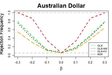
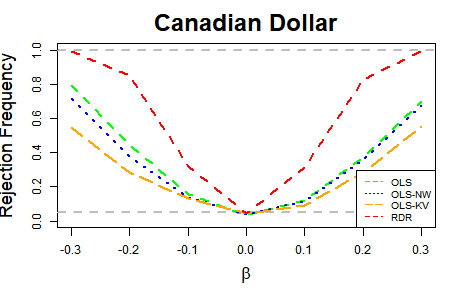
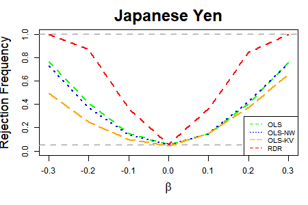
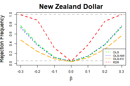
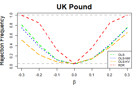
Figure 1: Size-corrected power for OLS (green), OLS-NW (blue), OLS-KV (yellow) and $RDynReg$ (red): A 5% t-test is conducted for the sample size T=250. The underlying model is the Hansen-Hodrick model (1980). The null value is $\beta=0$ and the alternatives are $\beta=\pm 0.1,\pm 0.2,\pm 0.3$.

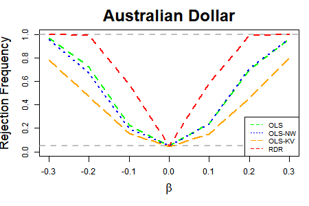
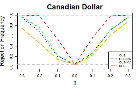
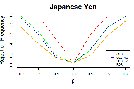
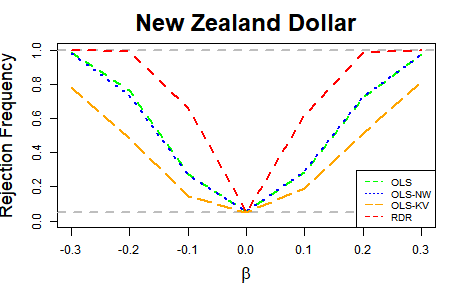
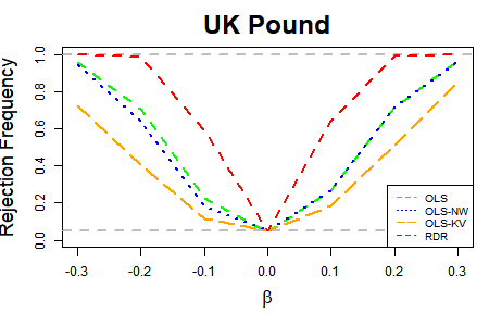
Figure 2: Size-corrected power for OLS (green), OLS-NW (blue), OLS-KV (yellow) and $RDynReg$ (red): A 5% t-test is conducted for the sample size T=500. The underlying model is the Hansen-Hodrick model (1980). The null value is $\beta=0$ and the alternatives are $\beta=\pm 0.1,\pm 0.2,\pm 0.3$.

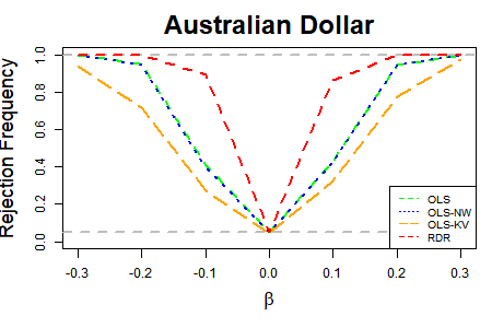
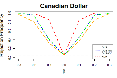
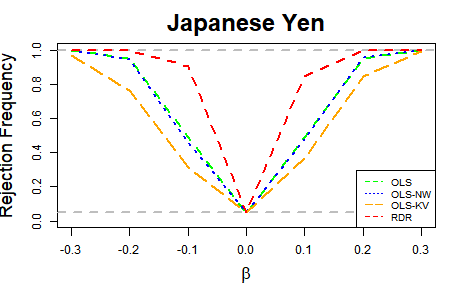
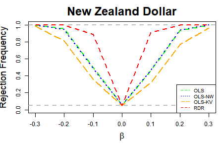
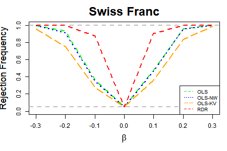
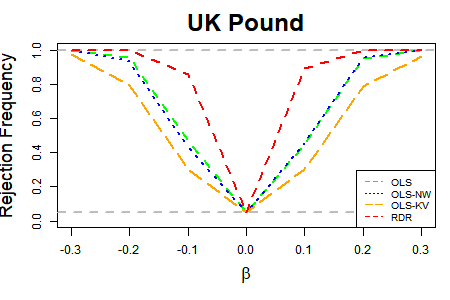
Figure 3: Size-corrected power for OLS (green), OLS-NW (blue), OLS-KV (yellow) and $RDynReg$ (red): A 5% t-test is conducted for the sample size T=1000. The underlying model is the Hansen-Hodrick (1980) model. The null value is $\beta=0$ and the alternatives are $\beta=\pm 0.1,\pm 0.2,\pm 0.3$.

Finally, the simulation results of Figures 1–3 we show size-corrected power curves for sample sizes $T=250$, $T=500$ and $T=1,000$, respectively, for $\beta\in[-0.3,0.3]$. $DynReg$ clearly dominates, for all six currencies. The high $DynReg$ test power is a natural consequence of its higher estimation efficiency.

In summary, Table 1 and Figures 1–3 clearly indicate that the $DynReg$ and $RDynReg$ methods improve on all competitors in all dimensions.

4 Empirical Results for Six Currencies

The above methodology was also implemented on the same weekly spot exchange rate data between January $1989$ through April $2021$ and were complemented with the actual $30$ day forward rate data which was recorded on the Tuesday of each week. This provides $T=1,941$ observations for each bi-variate system for each of the six currencies. In practice, due to the occurrence of holidays, religious festivals, and weekends, all of which produce market closures, the length of time between a forward rate and its corresponding spot rate in the data set is between $19$ and $25$ days.

There are several sets of results; each of which includes both $OLS/HAC$ and $DynReg$ estimation. Table 2 presents results for the model in equation (6), where the forward rate forecast error is regressed on its lagged value. The $OLS/HAC$ results have positive but small values for the estimated $\beta$ with significant rejections of the $\beta=0$ null for all countries apart from Switzerland. The $DynReg$ results uniformly do not reject the null.

The more interesting results appear in Table 3. They are based on the classic Fama forward premium regression (3), which has more economic and financial intuition. The $OLS/HAC$ $\beta$ estimates are between 0.07 for Canada and -0.11 for Japan. Three of the currencies have an estimated $\beta<0$, which is the case originally emphasized by Fama (1984). None of these six estimated $\beta$ coefficients are significantly different from zero at conventional levels. However, the results of $DynReg$ estimation indicate long-run $\beta$ in the range of 0.24 to 0.31 while the restricted $RDynReg$ are in the range of 0.30 to 0.40 for all six currencies. Hence the $DynReg$ results all indicate significant risk premia but less than those of early studies with monthly data where the $\beta<0.$

The appropriate Likelihood Ratio ($LR$) test statistic for the hypothesis of $UIP$ is denoted by $\lambda_{LR}$ and shows overwhelming rejections of the $UIP$ and $EMH$ for all six currencies. Hence this indicates the importance of information in the lagged forward rate errors, which is likely due to time variation in the risk premium.

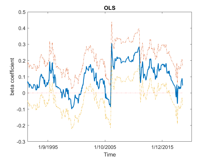
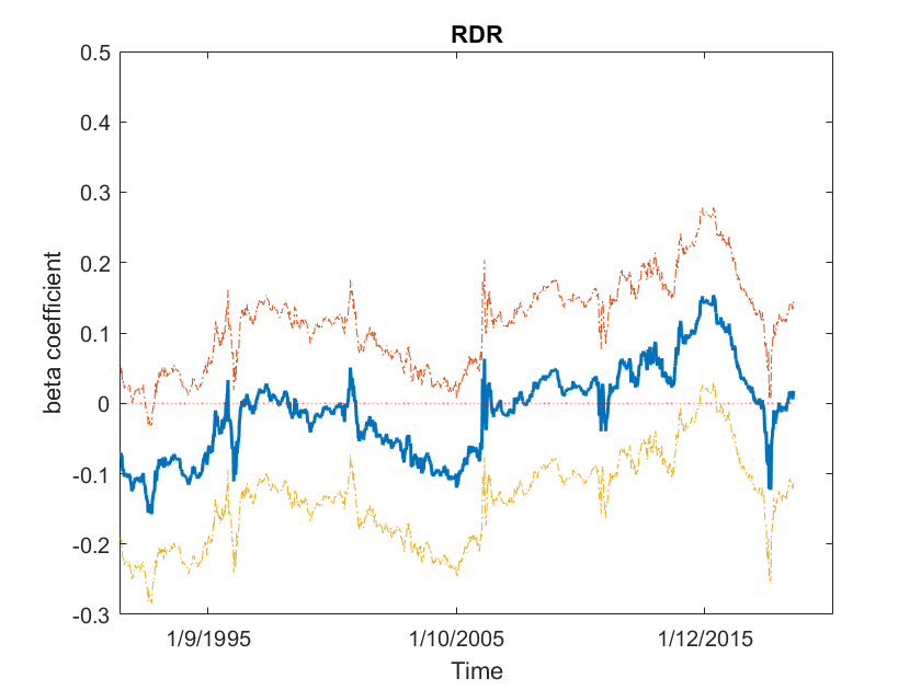
Australian Dollar	Australian Dollar
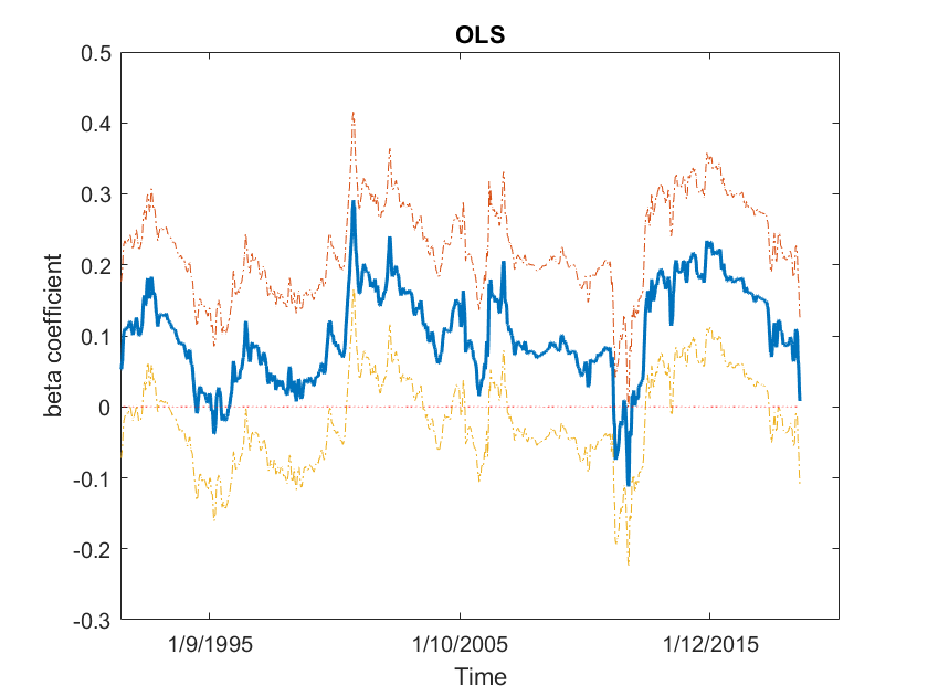
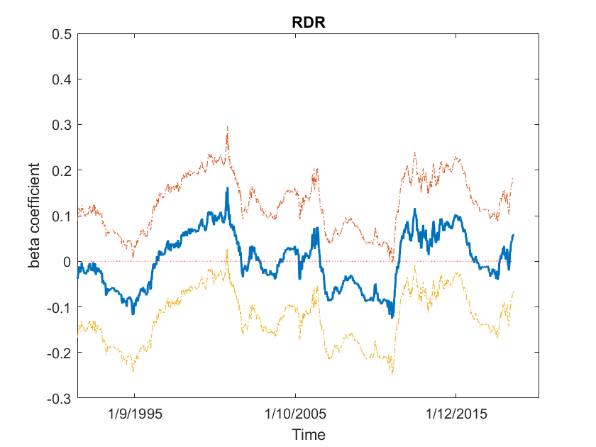
Canadian Dollar	Canadian Dollar
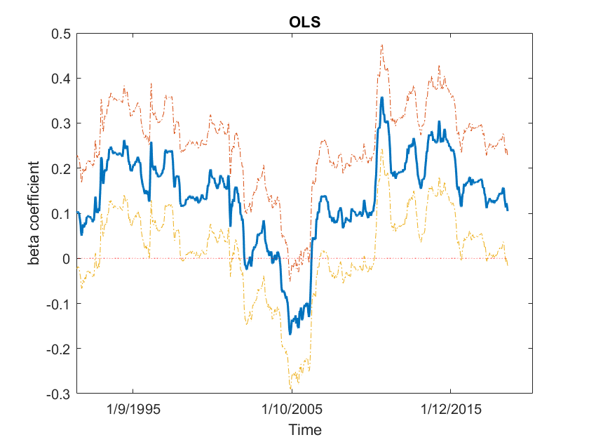
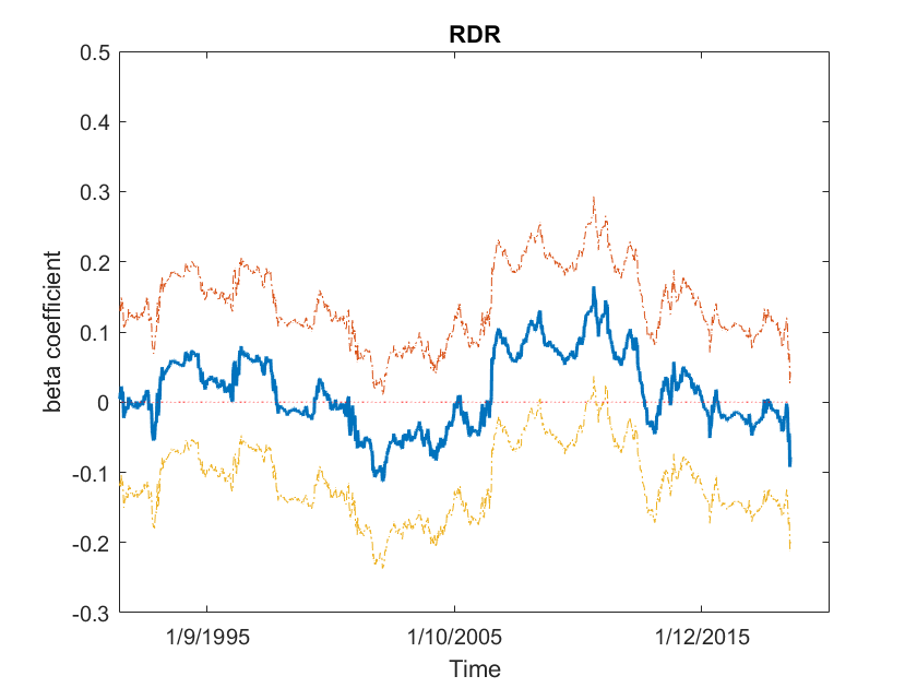
Japanese Yen	Japanese Yen

Figure 4: The blue curve is the 5-year rolling OLS (left)/$RDynReg$ (right) estimate of $\beta$ in the Hansen-Hodrick (1980) model; The null is $\beta=0$ and the dashed ones are the 95% confidence bands.

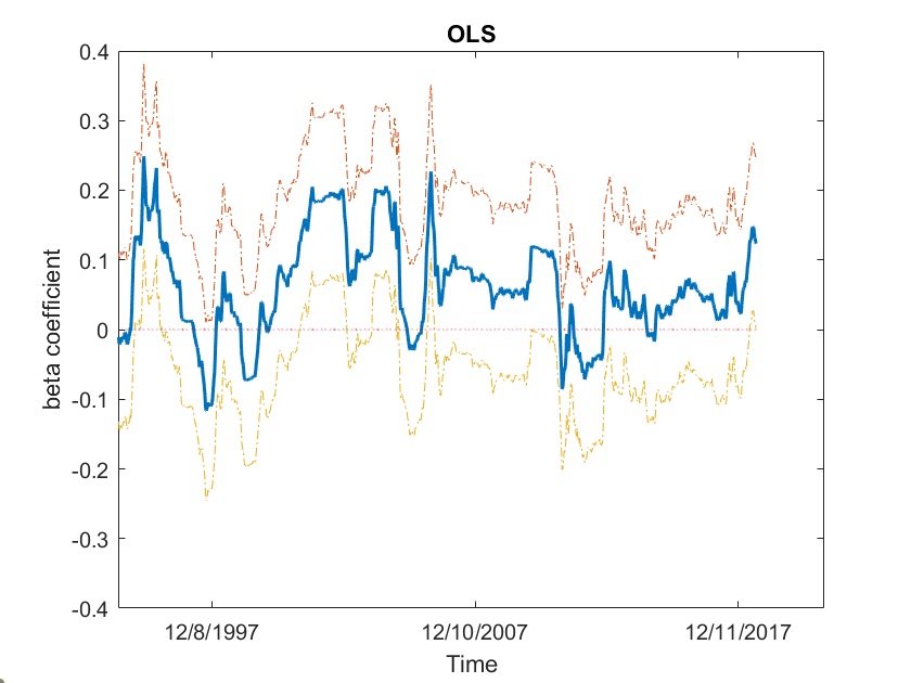
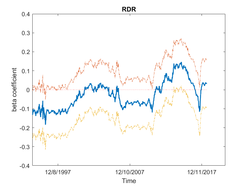
New Zealand Dollar	New Zealand Dollar
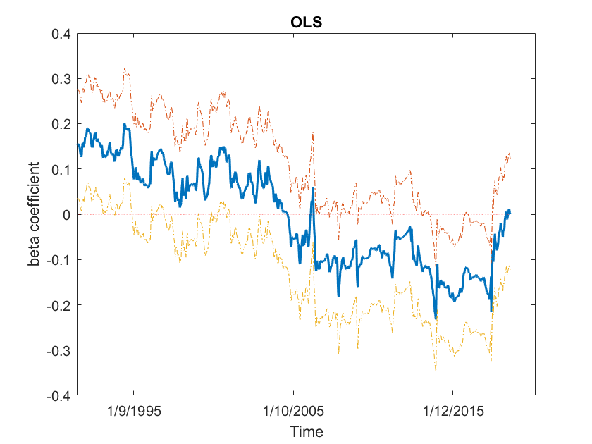
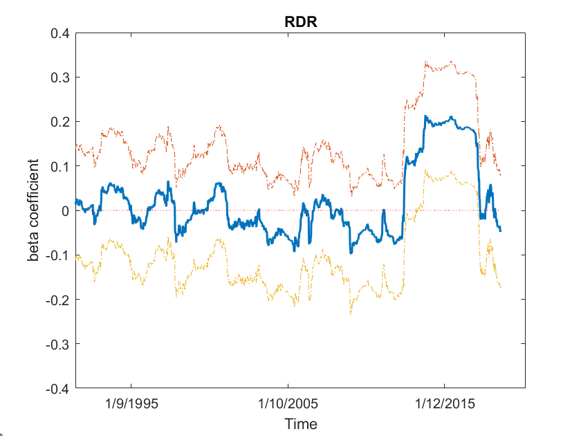
Swiss Franc	Swiss Franc
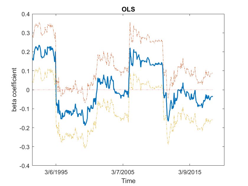
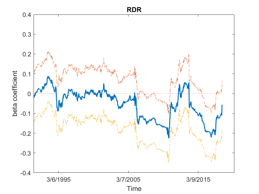
UK Pound	UK Pound

Figure 5: The blue curve is the 5-year rolling OLS (left)/$RDynReg$ (right) estimate of $\beta$ in the Hansen-Hodrick (1980) model; The null is $\beta=0$ and the dashed ones are the 95% confidence bands.

Some further insights into testing the $UIP$ condition are obtained by estimating the above models with five years of observations in each rolling sample. The results are reported graphically in Figures 4 through 7. Figures 4 and 5 show the estimates of $\beta$ from the forward rate forecast error regressions.  The $OLS$ estimates in the left hand panel are considerably more jagged and rough than those of the long run beta estimated by $DynReg$ in the right hand set of panels. The estimates of long run $\beta$ do not significantly depart from zero in any case. The 95% confidence bands for $DynReg$ almost entirely contain the null in the Hansen-Hodrick model (i.e. $\beta=0$) for Australian Dollar, Canadian Dollar, Japanese Yen and New Zealand Dollar (i.e. Figs 4 and 5). For Swiss Franc and UK Pound, the band mostly covers the null value. This is clearly not the case with OLS.

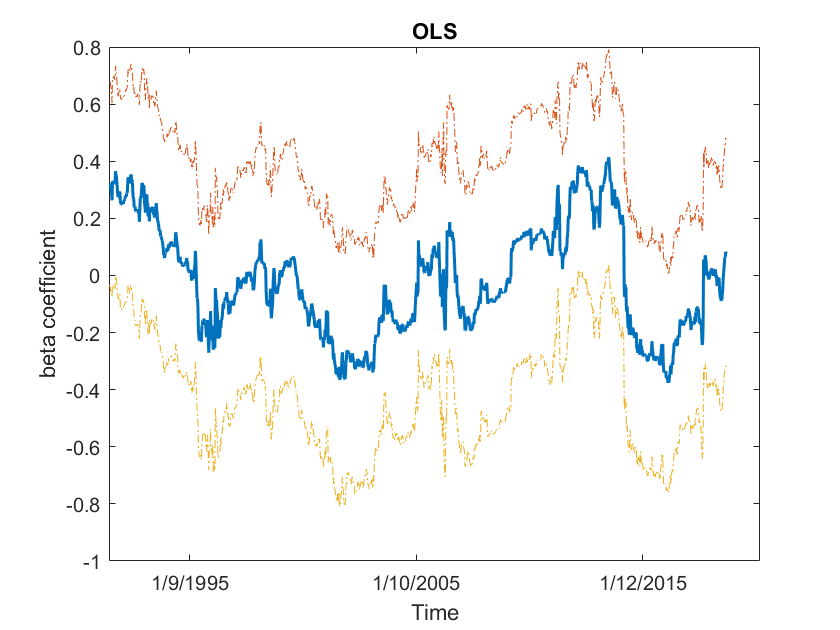
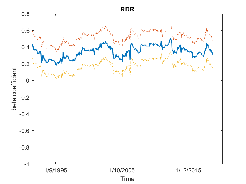
Australian Dollar	Australian Dollar
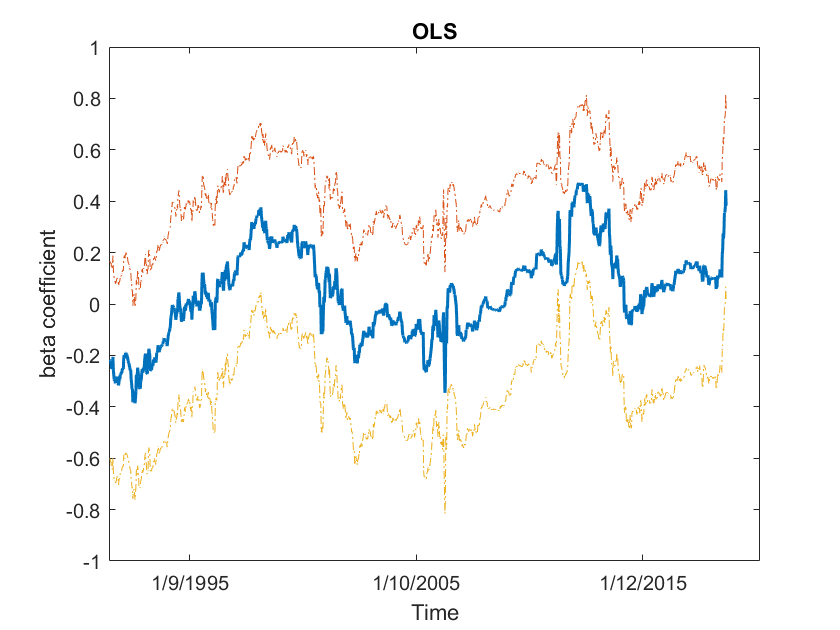
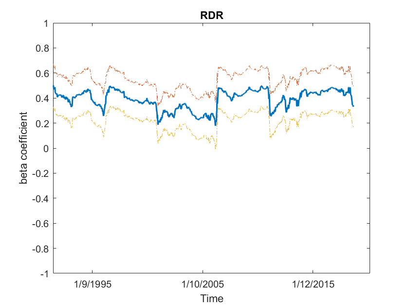
Canadian Dollar	Canadian Dollar
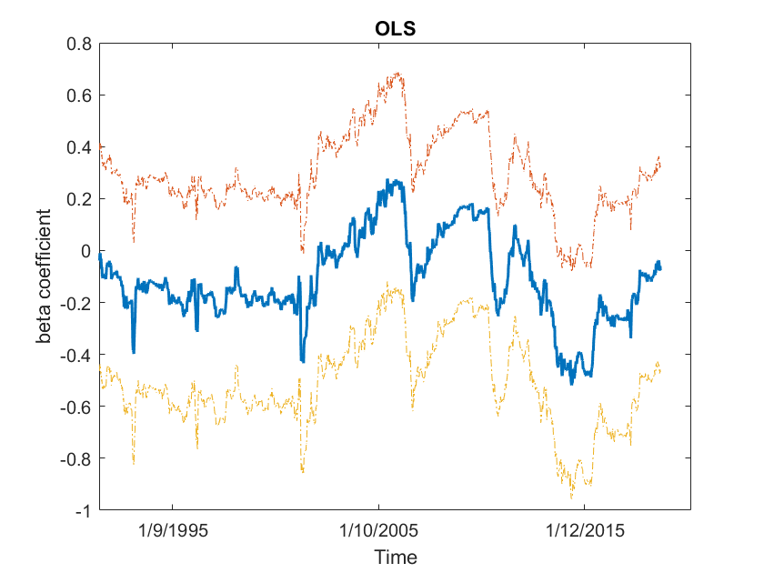
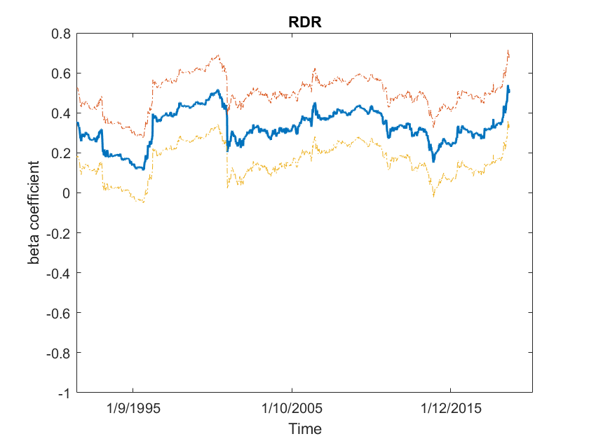
Japanese Yen	(f) Japanese Yen

Figure 6: The blue curve is the 5-year rolling OLS (left)/$RDynReg$ (right) estimate of $\beta$ in the Fama (1984) model; The null is $\beta=1$ and the dashed ones are the 95% confidence bands.

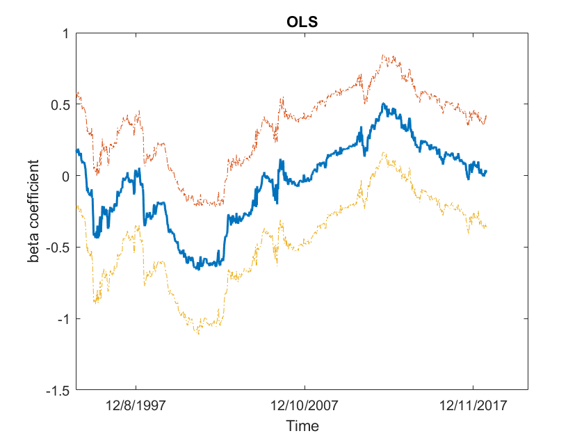
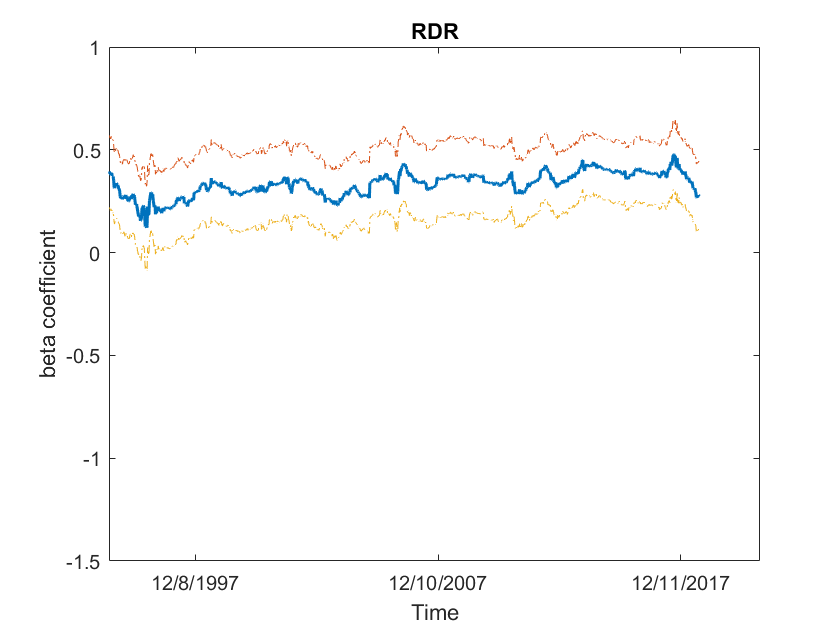
New Zealand Dollar	New Zealand Dollar
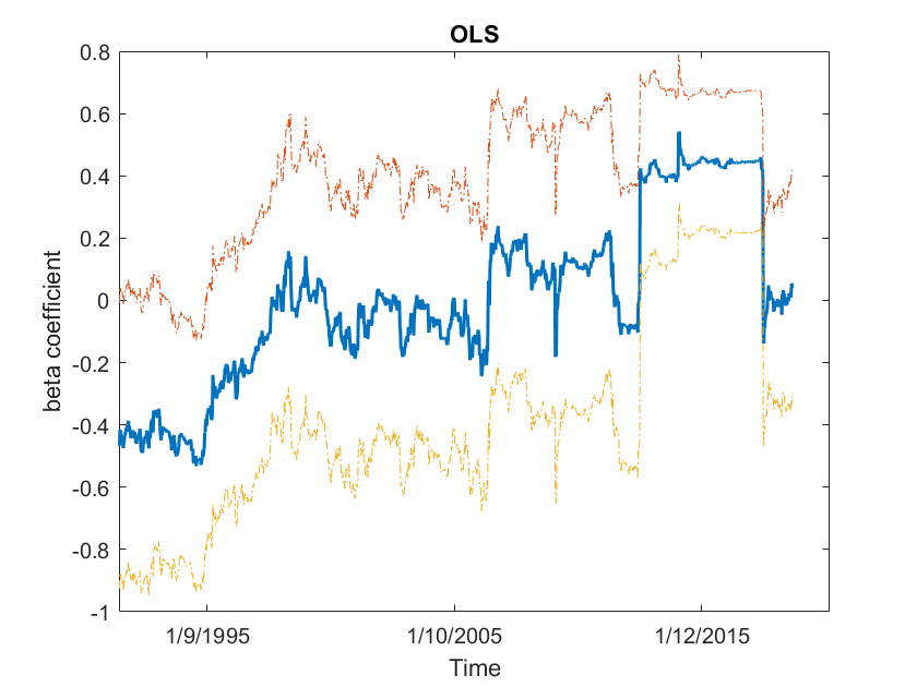
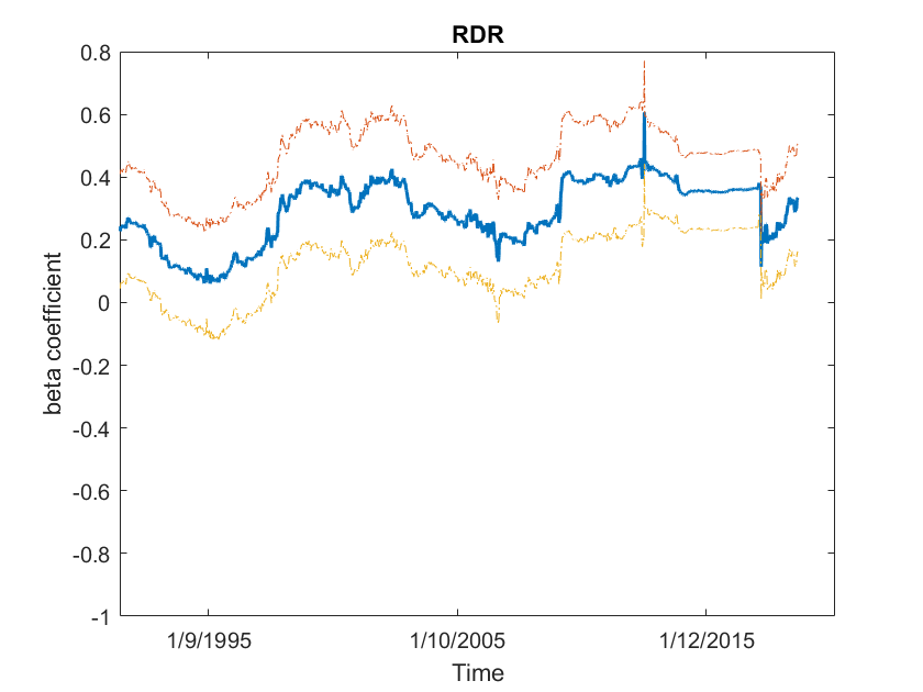
Swiss Franc	Swiss Franc
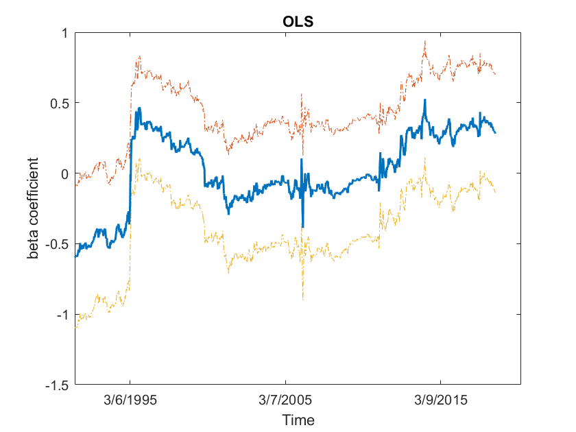
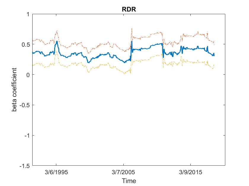
UK Pound	UK Pound

Figure 7: The blue curve is the 5-year rolling OLS (left)/$RDynReg$ (right) estimate of $\beta$ in the Fama (1984) model; The null is $\beta=1$ and the dashed ones are the 95% confidence bands.

The results for the Fama regression in (5), shown by Figs 6 and 7, are particularly interesting and indicate considerable stability over the rolling sample from the $DynReg$ estimates. These estimates are all positive and are typically around 0.4 instead of the $\beta=1$ implied by $UIP$. Given that the confidence bands for the $DynReg$ estimates in Figs 6 and 7 stay above zero for all six currencies, the estimates are statistically different to zero for virtually all sets of rolling regressions, which is not the case with $OLS$. Switzerland has slightly increased $\beta$ during the financial crisis and is otherwise quite stable. New Zealand has a slightly lower $\beta$ value than the other currencies.

Hence there is considerable evidence that the $UIP$ condition needs to be appended with risk premium terms, or possibly some measure of informational inefficiency. Models with appropriate variables could potentially be included in the modeling framework introduced in this paper.

5 Conclusions

This paper has suggested a new single-equation test for $UIP$ and $EMH$ based on $OLS$ estimation of a dynamic regression. The approach provides consistent and asymptotically efficient parameter estimates, and is not dependent on assumptions of strict exogeneity. This new approach has the advantage of being asymptotically more efficient than the common approach of using $HAC$ robust standard errors in the static forward premium regression. The method also has advantages of showing dynamic effects of risk premia, or other events that may lead to rejection of $UIP$ and $EMH$. The empirical results when spot returns are regressed on the lagged forward premium are all positive and remarkably stable across currencies.

Table 1: Performance of Tests of $\beta=0$ in Dynamic Regressions versus $OLS$ with robust standard errors in the Hansen-Hodrick (1980) model:

$$s_{t+k}-f_{t}=\alpha+\beta(s_{t}-f_{t-k})+u_{t+k}.$$

Under $EMH$ that $H_{0}:\,\alpha=0$ and $\beta=0$ and $Cov(u_{t+k},\,u_{t+k-j})=0$ for $j>k$,

		Australian Dollar				Canadian Dollar
		Bias	MSE	Level		Bias	MSE	Level
OLS		-0.0054	0.0019	0.2630		-0.0034	0.0018	0.2620
OLS-HH		–	–	0.0660		–	–	0.0560
OLS-NW		–	–	0.0810		–	–	0.0760
OLS-Andrews		–	–	0.0760		–	–	0.0720
OLS-KV		–	–	0.0520		–	–	0.0540
OLS-EWC		–	–	0.0590		–	–	0.0660
$DynReg$		-0.0004	0.0012	0.0590		0.0010	0.0011	0.0570
$RDynReg$		-0.0018	0.0006	0.0550		-0.0004	0.0006	0.0460
		Japanese Yen				New Zealand Dollar
		Bias	MSE	Level		Bias	MSE	Level
OLS		-0.0054	0.0017	0.2470		-0.0021	0.0021	0.2880
OLS-HH		–	–	0.0650		–	–	0.0580
OLS-NW		–	–	0.0790		–	–	0.0780
OLS-Andrews		–	–	0.0760		–	–	0.0740
OLS-KV		–	–	0.0540		–	–	0.0620
OLS-EWC		–	–	0.0680		–	–	0.0660
$DynReg$		-0.0017	0.0011	0.0450		-0.0002	0.0012	0.0430
$RDynReg$		-0.0010	0.0006	0.0590		0.0004	0.0007	0.0550

Table 1: (Continued) Performance of Tests of $\beta=0$ in Dynamic Regressions versus $OLS$ with robust standard errors in the Hansen-Hodrick (1980) model:

$$s_{t+k}-f_{t}=\alpha+\beta(s_{t}-f_{t-k})+u_{t+k}.$$

Under $EMH$ that $H_{0}:\,\alpha=0$ and $\beta=0$ and $Cov(u_{t+k},\,u_{t+k-j})=0$ for $j>k$,

		Swiss Franc				UK Pound
		Bias	MSE	Level		Bias	MSE	Level
OLS		-0.0047	0.0017	0.2420		-0.0029	0.0018	0.2350
OLS-HH		–	–	0.0640		–	–	0.0650
OLS-NW		–	–	0.0720		–	–	0.0740
OLS-Andrews		–	–	0.0710		–	–	0.0740
OLS-KV		–	–	0.0440		–	–	0.0530
OLS-EWC		–	–	0.0610		–	–	0.0660
$DynReg$		-0.0001	0.0011	0.0470		-0.0008	0.0010	0.0390
$RDynReg$		-0.0015	0.0006	0.0480		-0.0003	0.0006	0.0460
Key: The first six test statistics are based on $OLS$ estimation of $\beta$ with standard errors based on estimated parameters estimated covariance matrix computed by (i) regular $OLS$, (ii) $HH$, method of Hansen and Hodrick, (iii) $NW$, method of Newey and West, (iv) $Andrews$, method of Andrews, (v) $KV$, method Kiefer and Vogelsang, (vi) $EWC$, Equally Weighted Cosine. The $DynReg$ statistics are based on estimation of the unrestricted dynamic regression in equation (16) and $RDynReg$ is the restricted dynamic regression in equation (19) that constrains the error to be an $MA$(k-1) process as defined in equation (12).

Table 2: Estimation of the Hansen-Hodrick (1980) model $s_{t+k}-f_{t}=\alpha+\beta(s_{t}-f_{t-k})+u_{t+k}$ for actual weekly spot and forward exchange rate data from January 1989 through April 2021.

		Australian Dollar				Canadian Dollar
		$\hat{\beta}$	$s.e.(\hat{\beta})$	$\lambda_{LR}$		$\hat{\beta}$	$s.e.(\hat{\beta})$	$\lambda_{LR}$
OLS		0.1393	0.0241	–		0.1210	0.0243	–
OLS-HH		–	0.0664	–		–	0.0536	–
OLS-NW		–	0.0606	–		–	0.0488	–
OLS-Andrews		–	0.0620	–		–	0.0479	–
OLS-KV		–	0.0158	–		–	0.0069	–
OLS-EWC		–	0.0566	–		–	0.0448	–
$DynReg$		-0.0776	0.0320	2408.6		-0.0167	0.0320	2226.6
$RDynReg$		0.0024	0.0245	–		-0.0003	0.0246	–
		Japanese Yen				New Zealand Dollar
		$\hat{\beta}$	$s.e.(\hat{\beta})$	$\lambda_{LR}$		$\hat{\beta}$	$s.e.(\hat{\beta})$	$\lambda_{LR}$
OLS		0.1503	0.0242	–		0.0955	0.0255	–
OLS-HH		–	0.0533	–		–	0.0598	–
OLS-NW		–	0.0483	–		–	0.0566	–
OLS-Andrews		–	0.0486	–		–	0.0582	–
OLS-KV		–	0.0098	–		–	0.0089	–
OLS-EWC		–	0.0497	–		–	0.0571	–
$DynReg$		0.0120	0.0324	2479.5		-0.0555	0.0338	2386.3
$RDynReg$		0.0192	0.0245	–		-0.0236	0.0258	–
		Swiss Franc				UK Pound
		$\hat{\beta}$	$s.e.(\hat{\beta})$	$\lambda_{LR}$		$\hat{\beta}$	$s.e.(\hat{\beta})$	$\lambda_{LR}$
OLS		0.0373	0.0244	–		0.0799	0.0244	–
OLS-HH		–	0.0474	–		–	0.0598	–
OLS-NW		–	0.0446	–		–	0.0540	–
OLS-Andrews		–	0.0455	–		–	0.0542	–
OLS-KV		–	0.0333	–		–	0.0158	–
OLS-EWC		–	0.0438	–		–	0.0576	–
$DynReg$		-0.0415	0.0322	2315.3		-0.0527	0.0321	2391.8
$RDynReg$		0.0280	0.0245	–		-0.0584	0.0245	–
Key: See key to Table 1. The Likelihood Ratio test statistic $\lambda_{LR}$ is from a test of the static $OLS$ regression model against the DynReg model.

Table 3: Estimation of the Fama (1984) model $s_{t+k}-s_{t}=\alpha+\beta(f_{t}-s_{t})+u_{t+k}$ for actual weekly spot and forward exchange rate data from January 1989 through April 2021.

		Australian Dollar				Canadian Dollar
		$\hat{\beta}$	$s.e.(\hat{\beta})$	$\lambda_{LR}$		$\hat{\beta}$	$s.e.(\hat{\beta})$	$\lambda_{LR}$
OLS		0.0115	0.0815	–		0.0727	0.0762	–
OLS-HH		–	0.1077	–		–	0.1124	–
OLS-NW		–	0.1055	–		–	0.1141	–
OLS-Andrews		–	0.1043	–		–	0.1129	–
OLS-KV		–	0.0300	–		–	0.0270	–
OLS-EWC		–	0.1068	–		–	0.1057	–
$DynReg$		0.2440	0.0503	2852.4		0.3038	0.0495	2669.7
$RDynReg$		0.3696	0.0340	–		0.3972	0.0325	–
		Japanese Yen				New Zealand Dollar
		$\hat{\beta}$	$s.e.(\hat{\beta})$	$\lambda_{LR}$		$\hat{\beta}$	$s.e.(\hat{\beta})$	$\lambda_{LR}$
OLS		-0.1148	0.0815	–		-0.0320	0.0842	–
OLS-HH		–	0.0971	–		–	0.0847	–
OLS-NW		–	0.0927	–		–	0.0898	–
OLS-Andrews		–	0.0907	–		–	0.0902	–
OLS-KV		–	0.0171	–		–	0.0639	–
OLS-EWC		–	0.0842	–		–	0.0877	–
$DynReg$		0.2750	0.0503	2847.1		0.2392	0.0514	2845.9
$RDynReg$		0.3462	0.0334	–		0.3398	0.0351	–
		Swiss Franc				UK Pound
		$\hat{\beta}$	$s.e.(\hat{\beta})$	$\lambda_{LR}$		$\hat{\beta}$	$s.e.(\hat{\beta})$	$\lambda_{LR}$
OLS		0.0277	0.0770	–		-0.0737	0.0861	–
OLS-HH		–	0.1545	–		–	0.1066	–
OLS-NW		–	0.1491	–		–	0.1075	–
OLS-Andrews		–	0.1489	–		–	0.1058	–
OLS-KV		–	0.0983	–		–	0.0725	–
OLS-EWC		–	0.1486	–		–	0.1142	–
$DynReg$		0.2427	0.0477	2796.6		0.3054	0.0503	2797.2
$RDynReg$		0.3012	0.0326	–		0.3566	0.0365	–
Key: See key to Table 1. The Likelihood Ratio test statistic $\lambda_{LR}$ is from a test of the static $OLS$ regression model against the $DynReg$ model.

References

- [1] Anderson, T., Bollerslev, T. 1995. Intraday Periodicity and Volatility Persistence in Financial Markets, Journal of Empirical Finance, 4, 115-158.
- [2] Baillie R T. 1989. Econometric tests of rationality and market efficiency. Econometric Reviews 8: 151-186.
- [3] Baillie R T, Bollerslev T. 1989. Common stochastic trends in a system of exchange rates. Journal of Finance, 44: 167-181.
- [4] Baillie R T, Diebold F X, Kapetanios G, Kim K H. 2022. On robust inference in time series regression. arXiv:2203.04080, March, under revision.
- [5] Baillie R T, Lippens R E, McMahon, P C. 1983. Testing rational expectations and efficiency in the foreign exchange market . Econometrica 51: 553-563.
- [6] Baillie R T, Osterberg W P. 1997. Central bank intervention and risk in the forward premium. Journal of International Economics. 43: 483-497.
- [7] Baillie R T, Kilic R, 2006. Do asymmetric and nonlinear adjustments explain the forward premium anomaly? Journal of International, Money and Finance. 25: 22-47.
- [8] Bilson J F O. 1981. The speculative efficiency hypothesis. Journal of Business. 54: 435-452.
- [9] Burnside C, 2011. The cross section of foreign currency risk premia and consumption growth risk: comment. American Economic Review. 101: 3456-3476.
- [10] Corbae D, Ouliaris S. 1988. Robust tests for unit roots in the foreign exchange market. Economic Letters. 22: 375-380.
- [11] Domowitz I, Hakkio C S. 1984. Conditional variance and the risk premium in the foreign exchange market, Journal of International Economics. 19: 47-66.
- [12] Fama E F, 1984. Spot and forward exchange rates. Journal of Monetary Economics. 19: 319-338.
- [13] Frenkel J A, 1977. The forward exchange rate, expectations and the demand for money: The German hyperinflation. American Economic Review. 64: 653-670.
- [14] Frenkel J A, 1979. Further evidence on expectations and the demand for money during the German hyperinflation. Journal of Monetary Economics. 5: 81-96.
- [15] Frenkel J A, Levich R M. 1975. Covered Interest Arbitrage: Unexploited Profits?. Journal of Political Economy. 83(2): 325-338.
- [16] Grenander U, 1981. Indirect Inference. Wiley, New York.
- [17] Hakkio C S, 1981. Expectations and the forward exchange rate. International Economic Review 22: 663-678.
- [18] Hannan E J, Deistler M, 1988. The Statistical Theory of Linear Systems. SIAM..
- [19] Hansen L P, Hodrick R J, 1980. Forward exchange rates as optimal predictors of future spot rates: an econometric analysis. Journal of Political Economy, 88, 829–853.
- [20] Hansen, L P, Hodrick, R J. 1983. Risk averse speculation in the forward foreign exchange market: An econometric analysis of linear models. Exchange Rates and International Economics, edited by Jacob A. Frenkel.
- [21] Hodrick R J. 1989. Risk, uncertainty and exchange rates Journal of Monetary Economics. 23: 433-459.
- [22] Ismailov A, Rossi B, 2021. Uncertainty and deviations from uncovered interest rate parity. Journal of International, Money and Finance. forthcoming.
- [23] Kaminsky G, Peruga R, 1990. Can a time varying risk premium explain excess returns in the forward markets for foreign exchange? Journal of International Economics, 28: 47-70.
- [24] Levy E, Nobay A R, 1986. The speculative efficiency hypothesis: A bivariate analysis. Economic Journal, Annual Supplement, 109-121.1991.
- [25] Newey W K, West K D, 1987. A simple positive semi definite heteroscedasticity and autocorrelation consistent covariance matrix. Econometrica 55: 703-708.
- [26] Newey W K, West K D, 1994. Automatic lag selection in covariance matrix estimation, Review of Economic Studies 61: 634–654.
- [27] Schwarz G E, 1978. Estimating the dimension of a model. Annals of Statistics 6: 641-464.
- [28] Taylor M P, 1987. Covered interest parity: A high-frequency high-quality data study. Economica 54: 429-438.