POLICE: Provably Optimal Linear Constraint Enforcement for
Deep Neural Networks

Abstract

Deep Neural Networks (DNNs) outshine alternative function approximators in many settings thanks to their modularity in composing any desired differentiable operator. The formed parametrized functional is then tuned to solve a task at hand from simple gradient descent. This modularity comes at the cost of making strict enforcement of constraints on DNNs, e.g. from a priori knowledge of the task, or from desired physical properties, an open challenge. In this paper we propose the first provable affine constraint enforcement method for DNNs that only requires minimal changes into a given DNN’s forward-pass, that is computationally friendly, and that leaves the optimization of the DNN’s parameter to be unconstrained, i.e. standard gradient-based method can be employed. Our method does not require any sampling and provably ensures that the DNN fulfills the affine constraint on a given input space’s region at any point during training, and testing. We coin this method POLICE, standing for Provably Optimal LInear Constraint Enforcement. Github:https://github.com/RandallBalestriero/POLICE

1 Introduction

Deep Neural Networks (DNNs) are compositions of interleaved linear and nonlinear operators forming a differentiable functional $f_{{\bm{\theta}}}$ governed by some parameters ${\bm{\theta}}$ [1]. DNNs are universal approximators, but so are many other alternatives e.g. Fourier series [2], kernel machines [3], and decision trees [4]. The strength of DNNs rather lies in the ability of the function $f_{{\bm{\theta}}}$ to quickly and relatively easily fit most encountered target functional $f^{*}$ –often known through a given and finite training set– only by performing gradient updates on its parameters ${\bm{\theta}}$ [5]. This success, combined with the development of software and hardware making DNNs’ training and inference efficient, have made DNNs the operator of choice for most tasks encountered in machine learning and pattern recognition [6].

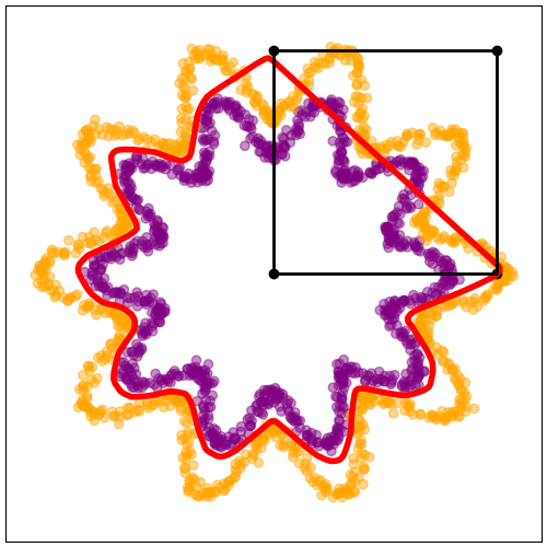
Fig. 1: Classification task of orange versus purple . The learned decision boundary ( red) comes from a SGD trained POLICEd DNN of depth $3$ with leaky-ReLU and dense layers of width $256$; POLICE provably enforce the DNN to be affine within the region delimited by the black lines through a simple projection of each layer’s bias parameters (Algorithm 1) –standard unconstrained optimization is still be used to train the DNN. See Fig. 2 for regression tasks.

Although ubiquitous for general purpose function fitting, DNNs have had a much harder time to shine in settings where specific constraints must be enforced exactly on the learned mapping. A motivating example follows from the following optimization problem

$$\min_{{\bm{\theta}}}\|f_{{\bm{\theta}}}-f^{*}\|+\lambda\mathcal{R}({\bm{\theta}})$$

$$\text{ s.t. }{\bm{J}}f_{{\bm{\theta}}}({\bm{x}})={\bm{A}},\forall{\bm{x}}\in R,$$ (1)

where ${\bm{J}}$ is the Jacobian operator and ${\bm{A}}$ is a target matrix that the model $f_{{\bm{\theta}}}$’s Jacobian should match for any input ${\bm{x}}$ in a given region $R$ of the input space. We employed explicitly a regularizer $\mathcal{R}$ with associated hyper-parameter $\lambda$ as one commonly employs weight-decay i.e. $\ell_{2}$ regularization on ${\bm{\theta}}$ [7]. The type of constraint of Eq. 1 is crucial in a variety of applications e.g. based on informed physical properties that $f_{{\bm{\theta}}}$ should obey [8, 9, 10] or based on (adversarial) noise robustness constraints [11, 12]. Another motivating example emerges when one has a priori knowledge that the target mapping $f^{*}$ is itself linear with parameters ${\bm{A}}^{*},{\bm{b}}^{*}$ within a region $R$ leading to the following optimization problem

$$\min_{{\bm{\theta}}}\|f_{{\bm{\theta}}}-f^{*}\|+\lambda\mathcal{R}({\bm{\theta}})$$

$$\text{ s.t. }f_{{\bm{\theta}}}({\bm{x}})={\bm{A}}^{*}{\bm{x}}+{\bm{b}}^{*},\forall{\bm{x}}\in R.$$ (2)

It is easy to see that one might arrive at numerous variants of Eqs. 1 and 2’s constraints. Crucial to our study is the observation that in all cases the necessary constraint one must provably and strictly enforce into $f_{{\bm{\theta}}}$ is to be affine within $R$. As a result, we summarize the generalized affine constraint that will interest us as follows

$$\min_{{\bm{\theta}}}\|f_{{\bm{\theta}}}-f^{*}\|+\lambda\mathcal{R}({\bm{\theta}})$$

$$\text{ s.t. }f_{{\bm{\theta}}}({\bm{x}})\text{ is affine on $R$},$$ (3)

and from which any more specific constraint can be efficiently enforced. For example, given Eq. 3, imposing Eq. 1 is straightforward by using a barrier method [13] with $\|{\bm{J}}f_{{\bm{\theta}}}({\bm{v}})-{\bm{A}}\|$ which can be done only by sampling a single sample ${\bm{v}}\in R$ and computing the DNN’s Jacobian matrix at that point. The same goes for imposing Eq. 2 given that Eq. 3 is fulfilled.

The main question that naturally arises is how to leverage DNNs while imposing Eq. 3. Current constraint enforcement with DNNs have so far only considered questions of verification [14, 15, 16] or constrained parameter space e.g. with integer parameters ${\bm{\theta}}$ [17] leaving us with little help to solve Eq. 3. A direct regularization-based approach suffers from the curse of dimensionality [18, 19] since sampling $R$ to ensure that $f_{{\bm{\theta}}}$ is affine requires exponentially many points as the dimension of $R$ increases. A more direct approach e.g. defining an alternative mapping $g_{{\bm{\theta}},{\bm{A}},{\bm{b}}}$ such as

$$g_{{\bm{\theta}},{\bm{A}},{\bm{b}}}({\bm{x}})=1_{\{{\bm{x}}\in R\}}({\bm{A}}{\bm{x}}+{\bm{b}})+1_{\{{\bm{x}}\not\in R\}}f_{{\bm{\theta}}}({\bm{x}}),$$

would destroy key properties such as continuity at the boundary $\partial R$. In short, we are in need of a principled and informed solution to strictly enforce Eq. 3 in arbitrarily wide and/or deep DNNs.

In this paper, we propose a theoretically motivated and provably optimal solution to enforce the affine constraint of Eq. 3 into DNNs. In particular, by focusing on convex polytopal regions $R$, we are able to exactly enforce the model to be affine on $R$; a visual depiction of the method at work is given in Fig. 1, and the pseudo-code is given in Algorithm 1. Our method has linear asymptotic complexity with respect to the number of vertices $P$ defining (or approximating) the region $R$ i.e. it has time-complexity $\mathcal{O}(KP)$ where $K$ is the complexity of the model’s forward pass. Hence the proposed strategy will often be unimpaired by the curse of dimensionality since for example a simplicial region $R\subset\mathbb{R}^{D}$ has only $D+1$ vertices [20] i.e. our method in this case has complexity growing linearly with the input space dimension. Our method is exact for any DNN architecture in which the nonlinearities are such as (leaky-)ReLU, absolute value, max-pooling and the likes, extension to smooth nonlinearities is discussed in Section 3. We coin our method POLICE standing for Provably Optimal LInear Constraint Enforcement; and we denoted a constrained DNN as being POLICEd. Two crucial benefits of POLICE are that the constraint enforcement is exact without requiring any sampling, and that the standard gradient-based training can be used on the POLICEd DNN parameters without any changes.

2 Strict Enforcement of Affine Constraints for Deep Neural Networks

In this section, we develop the proposed POLICE method that relies on two ingredients: (i) a DNN $f_{{\bm{\theta}}}$ using continuous piecewise-affine (CPA) nonlinearities which we formally introduce in Section 2.1; and (ii) a convex polytopal region $R$. The derivations of the proposed method will be carried in Section 2.2 and will empirically validated in Section 2.3.

2.1 Deep Neural Networks Are Continuous Piecewise Linear Operators

We denote the DNN input-output mapping as $f_{{\bm{\theta}}}:\mathbb{R}^{D}\mapsto\mathbb{R}^{K}$ with ${\bm{\theta}}$ the governing parameters of the mapping. In all generality, a DNN is formed by a composition of many layers as in

$$f_{{\bm{\theta}}}=\left(f_{{\bm{\theta}}^{(L)}}^{(L)}\circ\dots\circ f_{{\bm{\theta}}^{(1)}}^{(1)}\right),$$ (4)

where each layer mapping $f^{(\ell)}:\mathbb{R}^{D^{(\ell)}}\mapsto\mathbb{R}^{D^{(\ell+1)}}$ produces a feature map; with $D^{(1)}\triangleq D$ and $D^{(L)}\triangleq K$. For most architectures, i.e. parametrizations of the layers, the input-output mapping producing each feature map takes the form

$$f_{{\bm{\theta}}^{(\ell)}}^{(\ell)}({\bm{v}})=\sigma^{(\ell)}({\bm{h}}^{(\ell)}({\bm{v}}))\text{ with }{\bm{h}}^{(\ell)}({\bm{v}})={\bm{W}}^{(\ell)}{\bm{v}}+{\bm{b}}^{(\ell)}$$ (5)

where $\sigma$ is a pointwise activation function, ${\bm{W}}^{(\ell)}$ is a weight matrix of dimensions $D^{(\ell+1)}\times D^{(\ell)}$, and ${\bm{b}}^{(\ell)}$ is a bias vector of length $D^{(\ell+1)}$, ${\bm{h}}^{(\ell)}$ is denoted as the pre-activation map, and the layer parameters are gathered into ${\bm{\theta}}^{(\ell)}\triangleq\{{\bm{W}}^{(\ell)},{\bm{b}}^{(\ell)}\}$. The matrix ${\bm{W}}^{(\ell)}$ will often have a specific structure (e.g., circulant) at different layers. Without loss of generality we consider vectors as inputs since when dealing with images for example, one can always flatten them into vectors and reparametrize the layers accordingly leaving the input-output mapping of the DNN unchanged. The details on the layer mapping will not impact our results. One recent line of research that we will heavily rely on consists in formulating DNNs as Continuous Piecewise Affine (CPA) mappings [21, 22], that be expressed as

$$f_{{\bm{\theta}}}({\bm{x}})=\sum_{\omega\in\Omega}({\bm{A}}_{\omega}{\bm{x}}+{\bm{b}}_{\omega})1_{\{{\bm{x}}\in\omega\}},$$ (6)

where $\Omega$ is the input space partition induced by the DNN architecture, $\omega$ is a partition-region, and ${\bm{A}}_{\omega},{\bm{b}}_{\omega}$ are the corresponding per-region slope and offset parameters. A Key result that we will build upon is that the CPA formulation of Eq. 6 represents exactly the DNN functional of Eqs. 4 and 5, when the nonlinearities $\sigma$ are themselves CPA e.g. (leaky-)ReLU, absolute value, max-pooling [22].

2.2 POLICE Algorithm and Optimality

Equipped with the CPA notations expressing DNNs as per-region affine mappings (recall Eq. 6) we now derive the proposed POLICE algorithm that will strictly enforce the POLICEd DNN to fulfill the affine constraint from Eq. 3) on a region $R$ which is convex. We will then empirically validate the method in the following Section 2.3.

As mentioned above, our goal is to enforce the DNN to be a simple affine mapping on a convex region $R$. In particular, we will consider the $V$-representation of the region $R$ i.e. we consider $P$ vertices ${\bm{v}}_{1},\dots,{\bm{v}}_{P}$ so that the considered region $R$ is, or can be closely approximated by, the convex hull of those vertices as in

$$R=\left\{{\bm{V}}^{T}{\bm{\alpha}}:{\bm{\alpha}}_{p}\geq 0,\forall p\wedge{\bm{\alpha}}^{T}\mathbf{1}_{P}=1\right\},$$ (7)

where we gathered the $P$ vertices into the $P\times D$ matrix

$${\bm{V}}\triangleq[{\bm{v}}_{1},\dots,{\bm{v}}_{P}]^{T}.$$ (8)

We highlight that the actual ordering of the rows of ${\bm{V}}$ in Eq. 8, i.e. which vertex is put in which row, will not impact our result. We will also denote by ${\bm{v}}^{(\ell)}_{p}$ the $p^{\rm th}$ vertex mapped through the first $\ell-1$ layer, starting with ${\bm{v}}_{p}$ for $\ell=1$ and the corresponding matrix ${\bm{V}}^{(\ell)}$. By leveraging the CPA property of the DNN $f_{{\bm{\theta}}}$, one should notice that a necessary and sufficient condition for the model to stay affine within $R$ is to have the same pre-activation sign patterns (recall Eq. 5) which we formalize below.

Theorem 1.

A necessary and sufficient condition for a CPA DNN as per Eq. 6 to stay affine with a region $R$ given by Eq. 7 is to have the same pre-activation sign patterns between the vertices ${\bm{v}}_{p},\forall p\in[P]$ and that for each layer.

Proof.

The proof is direct. If the pre-activation signs are the same for all vertices, e.g. ${\rm sign}({\bm{h}}^{(1)}({\bm{v}}_{p}))={\rm sign}({\bm{h}}^{(1)}({\bm{v}}_{q}))$, $\forall p,q\in[P]^{2}$ for the first layer, then the vertices all lie within the same partition region i.e. $\exists\omega^{*}\in\Omega$ such that ${\bm{v}}_{p}\in\omega,\forall p$. Using Eq. 7 we obtain that $R\subset\omega^{*}$. Now, because the partition regions $\omega$ that form the DNN partition $\Omega$ (recall Eq. 6) are themselves convex polytopes, it implies that all the points within $\omega^{*}$, and thus $R$ since we showed that $R\subset\omega^{*}$, will also have the same pre-activation patterns, i.e. the entire DNN input-output mapping will stay affine within $R$ concluding the proof. ∎

Theorem 1 provides us with a necessary and sufficient condition but does not yet answer the principal question of “how to ensure that the vertices have the same pre-activation sign patterns”. There are actually many ways to enforce this, in our study we focus on one method that we deem the simplest and leave further comparison for future work.

Proposition 1.

A sufficient condition for layer $\ell$ to be linear within the input-space region defined by ${\bm{V}}$ (recall Eq. 8) is

$$0\leq\min_{(p,k)\in[P]\times[D^{(\ell+1)}]}{\bm{H}}_{p,k}{\bm{s}}_{k}$$ (9)

with ${\bm{H}}\triangleq{\bm{V}}^{(\ell)}({\bm{W}}^{(\ell)})^{T}+\mathbf{1}_{P}({\bm{b}}^{(\ell)})^{T}$ and with ${\bm{s}}_{k}$ being $1$ if $\#\{i:({\bm{H}})_{i,k}>0\}\geq P/2$ and $-1$ otherwise.

In the above, ${\bm{H}}$ is simply the pre-activation of layer $\ell$ given input ${\bm{V}}^{(\ell)}$, and Eq. 9 ensures that all vertices have the same sign pattern as ${\bm{s}}$; the latter determines on which side of the region ${\bm{V}}^{(\ell)}$ each hyperplane is projected to. Combining Theorems 1 and 1 leads to the POLICE algorithm given in Algorithm 1. Note that our choice of majority vote for ${\bm{s}}$ is arbitrary, other options would be valid as well depending on the desired properties that POLICE should follow. For example, one could find that direction based on margins instead. We now turn to empirically validate it in a variety of tasks in the following section.

Algorithm 1 POLICE procedure given a DNN $f_{{\bm{\theta}}}$ (recall Eq. 4) with activations $\sigma$ that can be (leaky-)ReLU or absolute value, and the region $R$ expressed by its vertices (recall Eq. 8). POLICE strictly enforces that $f_{{\bm{\theta}}}$ be affine in $R$; for clarity we denote by ${\rm MajorityVote}(.,{\rm axis}=0)$ the ${\bm{s}}$ vector from Proposition 1.

Train time procedure for each mini-batch ${\bm{X}}$:

1:${\bm{X}}\in\mathbb{R}^{N\times D},{\bm{V}}\in\mathbb{R}^{V\times D}$

2:${\bm{V}}^{(1)}\triangleq{\bm{V}},{\bm{X}}^{(1)}\triangleq{\bm{X}}$$\triangleright$ Initialization

3:for $\ell=1,\dots,L$ do$\triangleright$ Forward-pass

4:     ${\bm{H}}\leftarrow{\bm{V}}^{(\ell)}({\bm{W}}^{(\ell)})^{T}+\mathbf{1}_{P}({\bm{b}}^{(\ell)})^{T}$

5:     ${\bm{s}}={\rm MajorityVote}({\rm sign}({\bm{H}}),{\rm axis}=0)$

6:     ${\bm{c}}={\rm ReLU}(-{\bm{H}}{\rm diag}({\bm{s}})).{\rm max}({\rm axis}=0)\odot{\bm{s}}$

7:     ${\bm{X}}^{(\ell+1)}\leftarrow\sigma\left({\bm{X}}^{(\ell)}({\bm{W}}^{(\ell)})^{T}+\mathbf{1}_{N}({\bm{b}}^{(\ell)}+{\bm{c}})^{T}\right)$

8:     ${\bm{V}}^{(\ell+1)}\leftarrow\sigma\left({\bm{V}}^{(\ell)}({\bm{W}}^{(\ell)})^{T}+\mathbf{1}_{P}({\bm{b}}^{(\ell)}+{\bm{c}})^{T}\right)$

9:end for

10:${\bm{X}}^{(L)}$$\triangleright$ Evaluate loss and back-propagate as usual

Test time procedure (to run once post-training):

Do the train time procedure but without ${\bm{X}},{\bm{X}}^{(1)},\dots$ and set ${\bm{b}}^{(\ell)}\leftarrow{\bm{b}}^{(\ell)}+{\bm{c}},\forall\ell$ with ${\bm{c}}$ from Line 6.

target function

POLICE constrained

DNN approximation

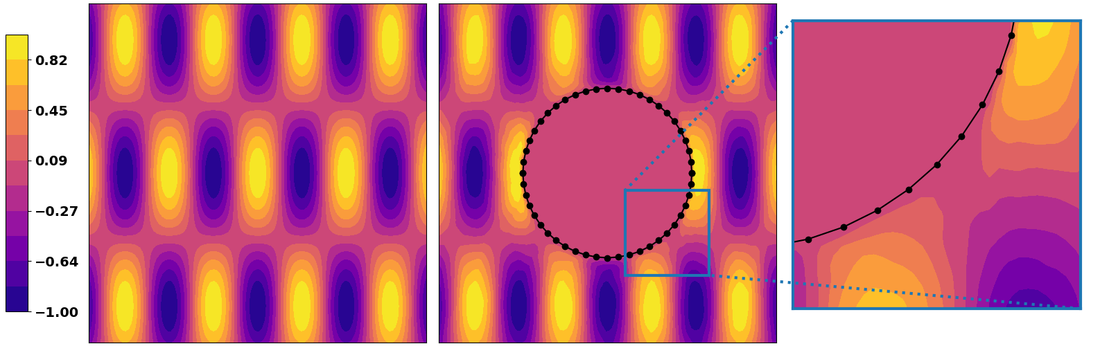
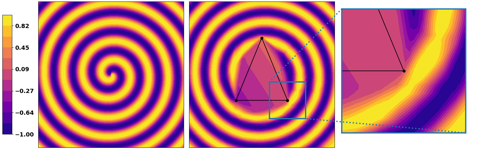
Fig. 2: Regression task of a $2$-dimensional space to a $1$-dimensional space with target function depicted in the left column with leaky-ReLU MLP of depth $4$ and width $256$ and for which the POLICE constrains the DNN to be an affine mapping within the region $R$ delimited by the black lines as depicted in the second column. On the right column a zoom-in is provided demonstrating how gradient based learning adapted the DNN parameters to very accurately approximate the target function.

Table 1: Average (over $1024$ runs) time (in ms.) and std to compute a forward-pass and a backward-pass with gradient accumulation in a standard DNN without any constraint enforced versus a POLICEd DNN for various input dimensions, widths and depths; given a mini-batch size of $1024$. We recall that at test time a POLICEd DNN has zero overhead (recall Algorithm 1).

input dim. $D$	2	2	2	784	784	3072
depth $L$	2.	4	4	2	8	6
widths $D^{(\ell)}$	256	64	4096	1024	1024	4096
no constr.	0.9$\pm$0	1.3$\pm$0	27.9$\pm$3	0.9$\pm$0	3.1$\pm$0	51.9$\pm$5
POLICEd	4.3$\pm$0	7.7$\pm$1	40.3$\pm$1	5.2$\pm$0	20.4$\pm$1	202.2$\pm$12
slow-down	$\times$4.5	$\times$ 5.7	$\times$ 1.4	$\times$ 5.5	$\times$ 6.6	$\times$ 3.9

2.3 Empirical Validation

We now propose to empirically validate the proposed POLICE method from Algorithm 1. First, we point out that POLICE can be applied regardless of the downstream task that one aims at solving e.g. classification or regression as presented in Figs. 1 and 2 respectively. In either case, the exact same methodology is employed (Algorithm 1). To complement the proposed classification case, we also provide in Fig. 3 the evolution of the DNN approximation at different training steps. We observe how the POLICE method enable gradient based learning to take into account the constraints so that the approximation can be of high-quality despite the constraint enforcement. Crucially, POLICE provides a strict constraint enforcement at any point during training requiring no tuning or sampling. We provide training times in Table 1 for the case with $R$ being the simplex of the considered ambient space, and recall the reader that POLICE has zero overhead at test time. We observe that especially as the dimension or the width of the model grows, as POLICE is able to provide relatively low computational overhead. In any case, the computational slow-down seems to lie between $1.4$ and $6.6$ in all studied cases. Additionally, those numbers were obtained from a naive Pytorch reproduction of Algorithm 1 and we expect the slow-down factor to greatly diminish by optimizing the implementation which we leave for future work.

target function

POLICE constrained DNN

step $5$

step $50$

step $10000$

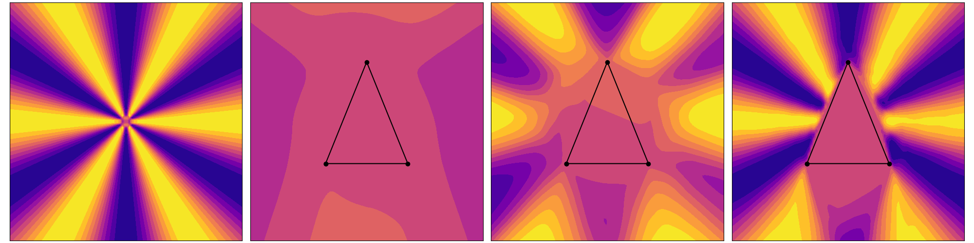
Fig. 3: Evolution of the DNN function approximation to the target function (left) at different training steps (5,50,10000) in each column. At any point during training POLICE strictly enforced the constraints on the region $R$ delimited by the black lines in a differentiable way to allow gradient based learning to discover a good value for the DNN parameters.

3 Conclusion and Future Work

We proposed a novel algorithm –POLICE– to provably enforce affine constraints into DNNs that employ continuous piecewise affine nonlinearities such as (leaky-)ReLU, absolute value or max-pooling. Given polytopal region $R$, POLICE enforces the DNN to be affine on $R$ only by a forward-pass through the DNN of the vertices defining $R$ (Algorithm 1) making it computationally efficient (Table 1) and lightweight to implement (no change in the model or optimizer). We believe that strict enforcement of the affine constraint is key to enable critical applications to leverage DNNs e.g. to enforce Eqs. 1 and 2. Among future directions we hope to explore the constraint enforcement on multiple regions simultaneously, and the extension to DNN employing smooth activation functions using a probabilistic argument as done e.g. in [24, 25]. Regarding the application of POLICE, we believe that implicit representation DNNs [26] could be fruitful beneficiaries.

References

- [1] Yann LeCun, Yoshua Bengio, and Geoffrey Hinton, “Deep learning,” nature, vol. 521, no. 7553, pp. 436–444, 2015.
- [2] Ronald Newbold Bracewell and Ronald N Bracewell, The Fourier transform and its applications, vol. 31999, McGraw-Hill New York, 1986.
- [3] Jooyoung Park and Irwin W Sandberg, “Universal approximation using radial-basis-function networks,” Neural computation, vol. 3, no. 2, pp. 246–257, 1991.
- [4] Mehryar Mohri, Afshin Rostamizadeh, and Ameet Talwalkar, Foundations of machine learning, MIT press, 2018.
- [5] Yann Le Cun, Ido Kanter, and Sara A Solla, “Eigenvalues of covariance matrices: Application to neural-network learning,” Physical Review Letters, vol. 66, no. 18, pp. 2396, 1991.
- [6] Ian Goodfellow, Yoshua Bengio, Aaron Courville, and Yoshua Bengio, Deep learning, vol. 1, MIT Press, 2016.
- [7] Anders Krogh and John Hertz, “A simple weight decay can improve generalization,” Advances in neural information processing systems, vol. 4, 1991.
- [8] Lipman Bers, Fritz John, and Martin Schechter, Partial differential equations, American Mathematical Soc., 1964.
- [9] Stanley J Farlow, Partial differential equations for scientists and engineers, Courier Corporation, 1993.
- [10] Lawrence C Evans, Partial differential equations, vol. 19, American Mathematical Soc., 2010.
- [11] Ian J Goodfellow, Jonathon Shlens, and Christian Szegedy, “Explaining and harnessing adversarial examples,” arXiv preprint arXiv:1412.6572, 2014.
- [12] Xiaoyong Yuan, Pan He, Qile Zhu, and Xiaolin Li, “Adversarial examples: Attacks and defenses for deep learning,” IEEE transactions on neural networks and learning systems, vol. 30, no. 9, pp. 2805–2824, 2019.
- [13] Anders Forsgren, Philip E Gill, and Margaret H Wright, “Interior methods for nonlinear optimization,” SIAM review, vol. 44, no. 4, pp. 525–597, 2002.
- [14] Youcheng Sun, Min Wu, Wenjie Ruan, Xiaowei Huang, Marta Kwiatkowska, and Daniel Kroening, “Concolic testing for deep neural networks,” in Proceedings of the 33rd ACM/IEEE International Conference on Automated Software Engineering, 2018, pp. 109–119.
- [15] Eric Wong and Zico Kolter, “Provable defenses against adversarial examples via the convex outer adversarial polytope,” in International Conference on Machine Learning. PMLR, 2018, pp. 5286–5295.
- [16] Changliu Liu, Tomer Arnon, Christopher Lazarus, Christopher Strong, Clark Barrett, Mykel J Kochenderfer, et al., “Algorithms for verifying deep neural networks,” Foundations and Trends® in Optimization, vol. 4, no. 3-4, pp. 244–404, 2021.
- [17] Shuang Wu, Guoqi Li, Feng Chen, and Luping Shi, “Training and inference with integers in deep neural networks,” arXiv preprint arXiv:1802.04680, 2018.
- [18] Richard E Bellman and Stuart E Dreyfus, Applied dynamic programming, vol. 2050, Princeton university press, 2015.
- [19] Mario Köppen, “The curse of dimensionality,” in 5th online world conference on soft computing in industrial applications (WSC5), 2000, vol. 1, pp. 4–8.
- [20] Herbert Edelsbrunner, Algorithms in combinatorial geometry, vol. 10, Springer Science & Business Media, 1987.
- [21] Guido F Montufar, Razvan Pascanu, Kyunghyun Cho, and Yoshua Bengio, “On the number of linear regions of deep neural networks,” Advances in neural information processing systems, vol. 27, 2014.
- [22] Randall Balestriero and Richard Baraniuk, “A spline theory of deep learning,” in International Conference on Machine Learning. PMLR, 2018, pp. 374–383.
- [23] Randall Balestriero, Romain Cosentino, Behnaam Aazhang, and Richard Baraniuk, “The geometry of deep networks: Power diagram subdivision,” Advances in Neural Information Processing Systems, vol. 32, 2019.
- [24] Randall Balestriero and Richard G Baraniuk, “From hard to soft: Understanding deep network nonlinearities via vector quantization and statistical inference,” arXiv preprint arXiv:1810.09274, 2018.
- [25] Ahmed Imtiaz Humayun, Randall Balestriero, and Richard Baraniuk, “Polarity sampling: Quality and diversity control of pre-trained generative networks via singular values,” in Proceedings of the IEEE/CVF Conference on Computer Vision and Pattern Recognition, 2022, pp. 10641–10650.
- [26] Vincent Sitzmann, Julien Martel, Alexander Bergman, David Lindell, and Gordon Wetzstein, “Implicit neural representations with periodic activation functions,” Advances in Neural Information Processing Systems, vol. 33, pp. 7462–7473, 2020.