The random Weierstrass zeta function II.
Fluctuations of the electric flux through rectifiable curves

Abstract

Consider a random planar point process whose law is invariant under planar isometries. We think of the process as a random distribution of point charges and consider the electric field generated by the charge distribution. In Part I of this work, we found a condition on the spectral side which characterizes when the field itself is invariant with a well-defined second-order structure. Here, we fix a process with an invariant field, and study the fluctuations of the flux through large arcs and curves in the plane. Under suitable conditions on the process and on the curve, denoted $\Gamma$, we show that the asymptotic variance of the flux through $R\,\Gamma$ grows like $R$ times the signed length of $\Gamma$. As a corollary, we find that the charge fluctuations in a dilated Jordan domain is asymptotic with the perimeter, provided only that the boundary is rectifiable.

The proof is based on the asymptotic analysis of a closely related quantity (the complex electric action of the field along a curve). A decisive role in the analysis is played by a signed version of the classical Ahlfors regularity condition.

1 Introduction

1.1 Electric fields and charge fluctuations

Denote by $\Lambda$ a stationary random point process in the complex plane ${\mathbb{C}}$ with intensity $c_{\Lambda}$ (i.e. the mean number of points of $\Lambda$ per unit area). If we think of $\Lambda$ as a random distribution of identical point charges, each sample generates an electric field which we identify with a solution $V_{\Lambda}$ to the equation

$$\bar{\partial}\,V_{\Lambda}=\pi\sum_{\lambda\in\Lambda}\delta_{\lambda}-\pi c_{\Lambda}\hskip 1.0ptm,$$ (1.1)

where $\bar{\partial}=\frac{1}{2}(\partial_{x}+{\rm i}\,\partial_{y})$ and where $m$ is the Lebesgue measure. In [21] (henceforth referred to as Part I), we found that, for processes with a spectral measure $\rho_{\Lambda}$, the spectral condition

$$\int_{|\xi|\leq 1}\frac{{\rm d}\rho_{\Lambda}(\xi)}{|\xi|^{2}}<\infty$$ (1.2)

characterizes those processes $\Lambda$ for which there exists a stationary electric field $V_{\Lambda}$ with a well-defined second-order (covariance) structure. When it exists, the field is given by

$$V_{\Lambda}(z)=\lim_{R\to\infty}\sum_{|\lambda|<R}\frac{1}{z-\lambda}-\pi c_{\Lambda}\hskip 1.0pt\overline{z},$$ (1.3)

and furthermore, it is essentially unique. In addition, the covariance structure of $V_{\Lambda}$ is conveniently expressed in terms of the covariance structure of $\Lambda$. The field $V_{\Lambda}$ can be seen as a random analogue of the Weierstrass zeta function from the theory of elliptic functions.

Denote by $n_{\Lambda}(\mathcal{G})=\#(\Lambda\cap\mathcal{G})$ the counting measure (or “charge”) of a Borel set $\mathcal{G}$. The asymptotic variance ${\sf Var}[n_{\Lambda}(R\mathcal{G})]$ of the charge fluctuations as $R\to\infty$ is of central interest in statistical physics. For the Poisson process, the size of the charge fluctuations in a disk is proportional to the area, while for more negatively correlated point processes the fluctuations tend to be suppressed and grow like $o(R^{2})$. Following Torquato-Stillinger, such processes are called hyperuniform or super-homogeneous; see [23]. Classical examples of hyperuniform point processes include the Ginibre ensemble [8] and the zero set of the Gaussian Entire Function (GEF) [3]. For both these examples, the variance of $n_{\Lambda}(R{\mathbb{D}})$ grows like the perimeter $R$. It is curious to ask to what extent the geometry of the disk is important, and in particular, what role is played by boundary regularity.

Since the divergence theorem expresses the charge in a domain as the electric flux through its boundary, it seems natural to ask for the behavior of the fluctuations of the flux of the field $V_{\Lambda}$ through more general rectifiable curves, which need not be closed nor simple. Specifically, given a rectifiable curve $\Gamma$ with unit normal $N$, we would like to describe the asymptotic variance of

$$\mathcal{F}_{\Lambda}(\Gamma)=\int_{R\Gamma}V_{\Lambda}(z)\cdot N\,|{\rm d}z|$$

for large $R$, provided that $\Lambda$ satisfies (1.2). To isolate the effect of the geometry of $\Gamma$, we will make the assumption that, in addition to being stationary, the law of the point process $\Lambda$ is invariant under rotations. We refer to such a process simply as “invariant”.

1.2 The electric action

For an invariant point process $\Lambda$ subject to the spectral condition (1.2), we introduce the electric action

$$\mathcal{E}_{\Lambda}(\Gamma)=\int_{\Gamma}V_{\Lambda}(z)\,{\rm d}z$$ (1.4)

where ${{\rm d}z}$ denotes the usual holomorphic $1$-differential and where $\Gamma$ is an arbitrary rectifiable curve in the plane. When $\Gamma$ bounds a Jordan domain $\mathcal{G}$, the action coincides with the flux, which in turn equals $2{\rm i}$ times $n_{\Lambda}(\mathcal{G})-c_{\Lambda}m(\mathcal{G})$. In general, if $T$ and $N$ denote the unit tangent and normal vectors to $\Gamma$, respectively, we obtain a decomposition

$$\mathcal{E}_{\Lambda}(\Gamma)=\int_{\Gamma}\Big{(}V_{\Lambda}\cdot T+{\rm i}\,V_{\Lambda}\cdot N\Big{)}\,|{\rm d}z|\overset{{\sf def}}{=}\mathcal{W}_{\Lambda}(\Gamma)+{\rm i}\,\mathcal{F}_{\Lambda}(\Gamma)$$

of $\mathcal{E}_{\Lambda}(\Gamma)$ in terms of the flux $\mathcal{F}_{\Lambda}(\Gamma)$ and the work $\mathcal{W}_{\Lambda}(\Gamma)$ of the field along $\Gamma$. While we are mainly interested in flux, the action appears to be more natural from an analytical point of view. Note that the work $\mathcal{W}_{\Lambda}(\Gamma)$ vanishes when the curve is closed. It appears that in the general situation, the fluctuations of $\mathcal{W}_{\Lambda}(R\Gamma)$ are negligible compared with those of the flux $\mathcal{F}_{\Lambda}(R\Gamma)$ (see Theorem 1.6 below).

1.3 Main results

We assume throughout that $\Lambda$ has a finite second moment, that is, that $\mathbb{E}\left[n_{\Lambda}(B)^{2}\right]<\infty$ for any bounded Borel set $B$. Under this assumption, there exists a measure $\kappa_{\Lambda}$ (the reduced covariance measure) with the property that

$${\sf Cov}\left[n_{\Lambda}(\varphi),n_{\Lambda}(\psi)\right]=\iint_{{\mathbb{C}}\times{\mathbb{C}}}\varphi(z)\,\overline{\psi(z^{\prime})}\,{\rm d}\kappa_{\Lambda}(z-z^{\prime})\,{\rm d}m(z)$$

for any test functions $\varphi,\psi\in C^{\infty}_{0}({\mathbb{C}})$, where $n_{\Lambda}(\varphi)$ is the standard linear statistic given by $n_{\Lambda}(\varphi)=\sum_{\lambda\in\Lambda}\varphi(\lambda)$. The spectral measure $\rho_{\Lambda}$ is the Fourier transform of $\kappa_{\Lambda}$ (understood in the sense of distributions).

We will also assume that the reduced truncated two-point measure $\tau_{\Lambda}\overset{{\sf def}}{=}\kappa_{\Lambda}-c_{\Lambda}\delta_{0}$ has a density $k_{\Lambda}$ with respect to planar Lebesgue measure (the truncated two-point function). Here, $c_{\Lambda}$ is the intensity of $\Lambda$, and $\delta_{0}$ is the unit point mass at the origin.

We recall also the standing assumption that the stationary point process $\Lambda$ is invariant, i.e., that the law of $\Lambda$ is invariant under all planar isometries. Under this assumption, the two-point function is automatically radially symmetric, so that

$$\kappa_{\Lambda}(z)=k_{\Lambda}(|z|)\,{\rm d}m(z)+c_{\Lambda}\delta_{0}(z).$$ (1.5)

Our results will require that $(1+t^{2})k_{\Lambda}(t)\in L^{1}({\mathbb{R}}_{\geq 0},{\rm d}t)$. Then, by [Part I, Remark 5.3], the spectral measure $\rho_{\Lambda}$ has a radial density $h_{\Lambda}$ which is $C^{1}$-smooth. Furthermore, if $\kappa_{\Lambda}({\mathbb{C}})=0$ (i.e., $\displaystyle\int_{{\mathbb{C}}}k_{\Lambda}(|z|)\,{\rm d}m(z)=-c_{\Lambda}$), we have the identity

$$\int_{0}^{\infty}k_{\Lambda}(t)\,t^{2}\,{\rm d}t=-\frac{1}{4\pi^{2}}\int_{0}^{\infty}\frac{h_{\Lambda}(\tau)}{\tau^{2}}\,{\rm d}\tau,$$ (1.6)

see Remark 5.1 below. Hence, the above moment assumption implies that $\rho_{\Lambda}$ satisfies the spectral condition (1.2).

By a curve we mean a continuous map $\Gamma:I\to{\mathbb{C}}$ of an interval $I$ into the plane. We identify two maps if they differ by pre-composition with an order-preserving homeomorphism of two intervals. We stress that $\Gamma$ need not be injective; if this is required we call the curve simple. The curve $\Gamma$ is said to be rectifiable if it has finite length

$$|\Gamma|=\sup_{t_{0}<t_{1}<\ldots<t_{n}}\sum_{j=1}^{n}\big{|}\Gamma(t_{j})-\Gamma(t_{j-1})\big{|}=\int_{I}|\gamma^{\prime}(t)|\,{\rm d}t<\infty,$$

where the supremum is taken over all partitions $a\leq t_{0}<t_{1}<\ldots<t_{n}\leq b$ of $I=[a,b]$, and where, without loss of generality, it is tacitly assumed that $\gamma$ is a Lipschitz parametrization of $\Gamma$, so that $\gamma^{\prime}$ exists a.e.. When no confusion should arise, we will abuse terminology somewhat and identify a curve with its image. When referring to a particular parametrization, we will use lowercase Greek letters, and write e.g. $\gamma:I\to\Gamma$.

The following regularity notion plays a key role in our analysis.

Definition 1.1 (Weak Ahlfors regularity).

We say that a rectifiable curve $\Gamma$ is weakly Ahlfors regular if there exists a constant $C_{\Gamma}<\infty$ such that

$$\left|\int_{\Gamma\cap D}{\rm d}z\right|\leq C_{\Gamma}|\partial D|,$$ (1.7)

for any Euclidean disk $D\subset{\mathbb{C}}$.

The terminology is borrowed from the classical Ahlfors regularity condition, which asks that

$$\int_{\Gamma\cap D}|{\rm d}z|\leq C_{\Gamma}|\partial D|.$$

While rectifiable Jordan curves may fail to be Ahlfors regular, it turns out that they are always weakly Ahlfors; see Lemma 3.1. Informally speaking, the weak Ahlfors condition is meant to prevent excessive spiralling near the end points of $\Gamma$, which appears to be the main obstruction to linear growth of charge fluctuations.

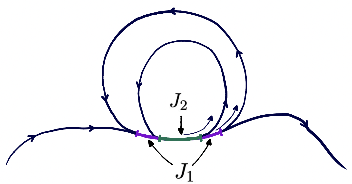
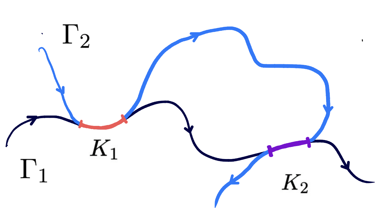
Figure 1: Left: The purple arcs $J_{1}\subset\Gamma$ are traversed twice and the green arc $J_{2}$ is traversed three times; these contribute $4\mathcal{H}^{1}(J_{1})$ and $9\mathcal{H}^{1}(J_{2})$, respectively, to the signed length $\mathcal{L}(\Gamma,\Gamma)$. Right: For the signed length $\mathcal{L}(\Gamma_{1},\Gamma_{2})$, the arc $K_{1}$ (orange) is counted with a positive sign, while $K_{2}$ (purple) is counted with negative sign.

Definition 1.2 (Signed length).

The signed length of the intersection of two rectifiable curves $\Gamma_{1}$ and $\Gamma_{2}$ is given by

$$\mathcal{L}(\Gamma_{1},\Gamma_{2})=\int_{{\mathbb{C}}}\bigg{(}\sum_{s\in\gamma_{1}^{-1}(z),\;t\in\gamma_{2}^{-1}(z)}\gamma_{1}^{\prime}(s)\cdot\gamma_{2}^{\prime}(t)\bigg{)}\,{\rm d}\mathcal{H}^{1}(z),$$ (1.8)

where $\gamma_{1}$ and $\gamma_{2}$ denote the arc-length parametrizations of the two curves, i.e. parametrizations with $|\gamma^{\prime}_{j}|=1$ a.e., and where $\mathcal{H}^{1}$ is one-dimensional Hausdorff measure on ${\mathbb{C}}$.

The quantity (1.8), which was introduced in [3], measures the length of the intersection $\Gamma_{1}\cap\Gamma_{2}$ taking orientation and multiplicity into account; see Figure 1. The signed length $\mathcal{L}(\Gamma_{1},\Gamma_{2})$ is finite for any two weakly Ahlfors regular curves; see Remark 3.3.

Theorem 1.3.

Denote by $\Lambda$ an invariant point process and let $\mathcal{E}_{\Lambda}(\Gamma)=\int_{\Gamma}V_{\Lambda}(z)\,{\rm d}z$. Assume that the two-point function $k_{\Lambda}$ of $\Lambda$ satisfies $(1+t^{2})k_{\Lambda}(t)\in L^{1}({\mathbb{R}}_{\geq 0},{\rm d}t)$ together with the zeroth moment condition

$$\int_{0}^{\infty}k_{\Lambda}(t)t\,{\rm d}t=-c_{\Lambda}.$$ (1.9)

Then, for any weakly Ahlfors regular rectifiable curves $\Gamma_{1}$ and $\Gamma_{2}$ we have that

$${\sf Cov}\big{[}\mathcal{E}_{\Lambda}(R\,\Gamma_{1})\,,\mathcal{E}_{\Lambda}(R\,\Gamma_{2})\big{]}=R\left(C_{\Lambda}+o(1)\right)\mathcal{L}(\Gamma_{1},\Gamma_{2})$$ (1.10)

as $R\to\infty$, where $\displaystyle{C_{\Lambda}=-8\pi^{2}\int_{0}^{\infty}k_{\Lambda}(t)\,t^{2}\,{\rm d}t}$.

Note that the identity (1.6) makes it clear that $C_{\Lambda}$ is positive. Since Jordan curves are always weakly Ahlfors regular (see Lemma 3.1), we get the following result.

Theorem 1.4.

Assume that $\Lambda$ satisfies the conditions of Theorem 1.3. Then for any Jordan domain $\mathcal{G}$ with rectifiable boundary, we have the asymptotics

$${\sf Var}\left[n_{\Lambda}(R\mathcal{G})\right]=\tfrac{1}{4}R\left(C_{\Lambda}+o(1)\right)|\partial\mathcal{G}|$$ (1.11)

as $R\to\infty$.

It should be mentioned that the fact that the zeroth-moment condition (1.9) yields the suppressed charge fluctuations (1.11) for domains $\mathcal{G}$ with smooth boundaries was known a long time ago, see [14, Section 1.6]

Remark 1.5.

Our proof of Theorem 1.3 yields that the weak Ahlfors condition can be relaxed to the maximal function criterion for the pair of rectifiable curves $(\Gamma_{1},\Gamma_{2})$:

$$\sup_{0<\varepsilon\leq 1}\varepsilon^{-1}\int_{0}^{\varepsilon}\frac{1}{t}\left|\int_{\Gamma_{1}\cap{\mathbb{D}}(\zeta,t)}{{\rm d}z}\right|{\rm d}t\in L^{1}(\Gamma_{2},|{\rm d}\zeta|)$$

without essential modifications. We have chosen to work with the stronger condition in Definition 1.1 to make the proofs as transparent as possible, but by doing so we miss out on a few examples where the maximal function condition would be needed. For instance, this seems to be the case for the “nested squares” curve $\Gamma_{1}=\Gamma_{2}=\bigcup_{k\geq 0}2^{-k}\partial Q$ where $Q=[0,1]\times[0,1]$.

There ought to exist counterexamples to the asymptotics of Theorem 1.3 if we do not impose anything like weak regularity. At least this is the case for the Ginibre ensemble, for which we show that for any $\varepsilon>0$, there exists a rectifiable Jordan arc $\Gamma_{\varepsilon}$ for which

$${\sf Var}\big{[}\mathcal{E}_{\Lambda}(R\Gamma_{\varepsilon})\big{]}\gtrsim R^{2-\varepsilon}|\Gamma|$$ (1.12)

holds as $R\to\infty$; see §6.1–§6.2.

Our last result concerns the asymptotics of the work $\mathcal{W}_{\Lambda}(\Gamma)$, i.e. the real part of the complex action $\mathcal{E}_{\Lambda}(\Gamma)$ (defined in §1.2).

Theorem 1.6.

Assume that the two-point function $k_{\Lambda}$ of the invariant point process $\Lambda$ satisfies $(1+t^{3})k_{\Lambda}(t)\in L^{1}({\mathbb{R}}_{\geq 0},{\rm d}t)$ along with the zeroth moment condition (1.9), and that $\Gamma$ is a weakly Ahlfors regular rectifiable curve with distinct start and end points. Then, as $R\to\infty$,

$${\sf Var}\big{[}\mathcal{W}_{\Lambda}(R\Gamma)\big{]}=\left(D_{\Lambda}+o(1)\right)\log R$$

where $\displaystyle{D_{\Lambda}=2\pi^{2}\int_{0}^{\infty}t^{3}k_{\Lambda}(t){\rm d}t}$. As a consequence, we have that, as $R\to\infty$,

$${\sf Var}\big{[}\mathcal{E}_{\Lambda}(R\Gamma)\big{]}={\sf Var}\big{[}\mathcal{F}_{\Lambda}(R\Gamma)\big{]}+O(\log R)\,.$$

In other words, under these assumptions the quantity $\mathcal{E}_{\Lambda}(R\Gamma)$ really measures the asymptotic electric flux through $R\Gamma$.

Remark 1.7.

Denoting by $(\Omega,\mathcal{F},\mathbb{P})$ the probability space on which the stationary point process $\Lambda$ is defined, let $\mathcal{F}_{\sf inv}\subset\mathcal{F}$ be the sigma-algebra of translation invariant events. Throughout this paper, we make the simplifying assumption that the spectral measure $\rho_{\Lambda}$ does not have an atom at the origin. As outlined in [Part I, §2.3], this is the same as saying that the conditional intensity of $\Lambda$, defined by

$$\mathfrak{c}_{\Lambda}=\pi^{-1}\mathbb{E}\big{[}n_{\Lambda}({\mathbb{D}})\mid\mathcal{F}_{{\sf inv}}\big{]}\,,$$

is non-random and equals $c_{\Lambda}$ almost surely. While this assumption simplifies the formulation of our results, our methods can be adapted to deal also with the case when $\rho_{\Lambda}(\{0\})>0$. We will not dwell on the details, but mention only that in this setting, the stationary vector field should be defined as in Part I by

$$V_{\Lambda}(z)=\lim_{R\to\infty}\sum_{|\lambda|<R}\frac{1}{z-\lambda}-\pi\mathfrak{c}_{\Lambda}\overline{z}\,,$$

and, in Theorem 1.4, one should replace the variance ${\sf Var}[n_{\Lambda}(R\,\mathcal{G})]$ with the re-centered variance ${\sf Var}\big{[}n_{\Lambda}(\mathcal{G})-\mathfrak{c}_{\Lambda}m(\mathcal{G})\big{]}$. Since the spectral measure $\rho_{V_{\Lambda}}$ and two-point function $K_{V_{\Lambda}}$ do not depend on the size of the atom $\rho_{\Lambda}(\{0\})$ ([Part I, Theorem 5.8]), only very minor modifications will be needed.

It is natural to ask about asymptotic normality of the renormalized electric flux $R^{-1/2}\mathcal{F}_{\Lambda}(R\Gamma)$ (or, equivalently, of the renormalized electric action). For the zeroes of GEFs and $C^{1}$-smooth curves, this was proven in [3] using the method of moments. An alternative is to use the clustering property of $k$-point functions (cf. Malyshev [13], Martin-Yalcin [15], Nazarov-Sodin [18, Theorem 1.5]), which is easy to verify for the Ginibre ensemble using its determinantal structure, and which was proven in [18] for the zero set of GEFs. We will not pursue the details here.

1.4 Related work

The study of charge fluctuations of stationary point processes is a classical topic in mathematical physics; see [6] for a recent survey. Important early contributions were the works of Martin-Yalcin [15], Lebowitz [11], and Jancovici-Lebowitz-Manificat [9] (see also Martin’s survey [14]). Recently there has been a resurgence of interest, due partly to the role of hyperuniform systems in material science (see e.g. [22]). This has highlighted the relationship between charge fluctuations and properties of the spectral measure; see the work [1] of Adhikari-Ghosh-Lebowitz and references therein for recent mathematical developments.

If we do not impose any smoothness condition on the spectral measure, there exist examples where the asymptotics (1.11) cease to hold. To see this, simply consider the stationary point process obtained by randomly shifting the lattice points $\mathbb{Z}^{2}\subset{\mathbb{R}}^{2}={\mathbb{C}}$ by a random variable uniformly distributed on $[0,1]^{2}$. In this example, the spectral measure consists of unit point masses on $\mathbb{Z}^{2}\setminus\{0\}$. Denoting by $\mathbb{B}^{p}\subset{\mathbb{R}}^{2}$ the unit ball in the $\ell^{p}$-metric, Kim and Torquato [10] showed that ${\sf Var}\big{[}n_{\Lambda}(R\,\mathbb{B}^{p})\big{]}$ grows like $R^{\sigma(p)}$, where $\sigma(p)$ varies continuously between $1$ and $2$ as $p$ ranges from $2$ to infinity. It is also worth mentioning that examples of this sort persists when considering independent Gaussian perturbations of the “randomly shifted” lattice, where the spectral measure is a mixture of an absolutely continuous part and a singular part, see Yakir [24]. Another related work is the recent study by Björklund and Hartnick [2], which investigated the hyperuniformity of various point processes which are models for quasicrystals. In this case the asymptotic of the number variance may depend on fine arithmetic properties of the quasicrystal.

For the zeros of the Gaussian Entire Function $F(z)$, the flux $\mathcal{F}_{\Lambda}(\Gamma)$ corresponds to the change in argument of $F(z)$ along $R\Gamma$. This was introduced by Buckley-Sodin in [3], though the idea was present already in Lebowitz work [11] on charge fluctuations in Coulomb systems. Buckley and Sodin obtained the large $R$-asymptotics of ${\sf Cov}\left[\mathcal{F}_{\Lambda}(R\Gamma_{1}),\mathcal{F}_{\Lambda}(R\Gamma_{2})\right]$ for piecewise $C^{1}$-regular curves $\Gamma_{1}$ and $\Gamma_{2}$ with a proof which used the properties of that ensemble. It is not clear whether the proof given there persists for weakly Ahlfors regular curves. We mention that the signed length recently appeared in the work of Notarnicola-Peccati-Vidotto on the length of nodal lines in Berry’s random planar wave model [19].

For determinental point processes (including the infinite Ginibre ensemble) Lin [12] very recently obtained a stronger version of Theorem 1.4, which is valid for a more general class of domains $\mathcal{G}$ having a bounded perimeter. He also showed that for a very large class of domains $\mathcal{G}$, ${\sf Var}\big{[}n_{\Lambda}(R\mathcal{G})\big{]}$ is comparable to $R^{\alpha(\mathcal{G})}$, where $\alpha(\mathcal{G})$ is the Minkowski dimension of $\partial\cal G$. Lin’s approach is based on the study of asymptotics of the functional

$$\iint_{{\mathbb{R}}^{2}\times{\mathbb{R}}^{2}}\big{(}{1\hskip-2.5pt{\rm l}}_{\mathcal{G}}(x)-{1\hskip-2.5pt{\rm l}}_{\mathcal{G}}(y)\big{)}^{2} \rho\big{(}R|x-y|\big{)}\,{\rm d}m(x)\,{\rm d}m(y)$$

$$=\iint_{\mathcal{G}\times\mathcal{G}^{c}}\rho\big{(}R|x-y|\big{)}\,{\rm d}m(x)\,{\rm d}m(y)$$

as $R\to\infty$, where $\rho$ is a non-negative integrable function which is sufficiently fast decaying at infinity (cf. Dávila [4]). In our case $\rho=-k_{\Lambda}$, the (truncated) two-point function of $\Lambda$ taken with negative sign. Non-negativity of $\rho$ seems to be an obstacle for using this technique for non-determinental point processes. Nevertheless, Lin mentions [12, Remark 1.2.3] that his techniques can be also applied to zeros of Gaussian Entire Functions.

There is also a resemblance between the topic of this paper and the study of “irregularities of distribution” e.g. in the work of Montgomery [17, Ch. 6].

1.5 Outline of the paper

The starting point for the asymptotic analysis of ${\sf Var}\big{[}\mathcal{E}_{\Lambda}(R\Gamma)\big{]}$ is the identity

$${\sf Var}\big{[}\mathcal{E}_{\Lambda}(R\Gamma)\big{]}={\sf p.v.}\iint_{R\Gamma\times R\Gamma}K(|x-y|)\,{\rm d}x{\rm d}\bar{y},$$ (1.13)

where $K$ is the (singular) covariance kernel of $V_{\Lambda}$ (see §4) and where the principal value integral is understood in the sense of the limit

$$\lim_{\varepsilon\to 0}\iint_{R\Gamma\times R\Gamma}{1\hskip-2.5pt{\rm l}}_{\{|x-y|>\varepsilon\}}K(|x-y|)\,{\rm d}x{\rm d}\bar{y}.$$

The article is organized as follows. In §2 we recall various preliminaries, mainly on the second-order structure of stationary processes. Section 3 is devoted to geometric observations concerning the weak-Ahlfors condition. In §4 we establish the formula (1.13) for the variance and recall a convenient representation of the kernel $K$ from Part I. The proof of the main results are given in §5, and the existence of rectifiable but not weakly Ahlfors regular Jordan arcs with large charge fluctuations is discussed in §6 (this is made rigorous for the infinite Ginibre ensemble).

2 Preliminaries

2.1 Notation and conventions

We will frequently use the following notation.

• ${\mathbb{C}}$, ${\mathbb{R}}$, ${\mathbb{R}}_{\geq 0}$; the complex plane, the real line and the half line ${\mathbb{R}}_{\geq 0}=\{x\in{\mathbb{R}}:x\geq 0\}$

• ${\mathbb{D}}(x,R)$; the disk $\{z\in{\mathbb{C}}:|z-x|<R\}$. We let ${\mathbb{D}}(0,1)={\mathbb{D}}$

• $\partial=\partial_{z}$ and $\bar{\partial}=\partial_{\bar{z}}$; the Wirtinger derivatives

  $$\partial=\frac{1}{2}\left(\frac{\partial}{\partial x}-{\rm i}\frac{\partial}{\partial y}\right),\qquad\bar{\partial}=\frac{1}{2}\left(\frac{\partial}{\partial x}+{\rm i}\frac{\partial}{\partial y}\right)$$

• $m$; the Lebesgue measure on ${\mathbb{C}}$

• $\widehat{f}$; the Fourier transform, with the normalization

  $$\widehat{f}(\xi)=\int_{{\mathbb{C}}}\,e^{-2\pi{\rm i}x\cdot\xi}f(x)\,{{\rm d}}m(x)$$

• $\mathfrak{D}$, $\mathcal{S}$; the class of compactly supported $C^{\infty}$-smooth functions and the class of Schwartz functions, respectively

• $\mathbb{E}$, ${\sf Cov}$, ${\sf Var}$; the expectation, covariance and variance with respect to the probability space $(\Omega,\mathcal{F},\mathbb{P})$ on which $\Lambda$ is defined

• $K$; the two-point function for the stationary field $V_{\Lambda}$; see Lemma 4.1.

• $\rho_{\Lambda}$, $\kappa_{\Lambda}$, $\tau_{\Lambda}$; spectral measure, and the reduced and reduced truncated covariance measures for $\Lambda$; see §2.2.

• $c_{\Lambda}$; the intensity of $\Lambda$

• $\tau(x)=\tau_{\Gamma}(x)$; the “net tangent” $\tau(x)\overset{{\sf def}}{=}\sum_{t\in\gamma^{-1}(x)}\gamma^{\prime}(t)$ for an oriented rectifiable curve $\Gamma$; see (3.4)

• $n_{\Lambda}$; the random counting measure $n_{\Lambda}=\sum_{\lambda\in\Lambda}\delta_{\lambda}$

• $\mu(f)=(f,\mu)$; the distributional action of the measure $\mu$; i.e. $\mu(f)=\int f\,{{\rm d}\mu}$

• $\nu_{\Gamma}$; the current which acts on one-forms $\omega$ by $\nu_{\Gamma}(\omega)=\int_{\Gamma}{{\rm d}}\omega$. By a slight abuse of notation, we will write $\nu_{\Gamma}(f)$ to mean $\nu_{\Gamma}(f\,{\rm d}z)$. We will identify $\nu_{\Gamma}$ with a complex-valued finite measure by setting $\nu_{\Gamma}(B)=\int_{\Gamma\cap B}{\rm d}z$ for Borel sets $B\subset{\mathbb{C}}$.

• $\phi_{\varepsilon}$; the Gaussian $\phi_{\varepsilon}(z)=\frac{1}{\pi\varepsilon^{2}}e^{-|z|^{2}/\varepsilon^{2}}$.

We use the standard $O$-notation and the notation $\lesssim$ with interchangeable meaning. If a limiting procedure involves an auxiliary parameter $a$, we write e.g. $f_{a}(x)=O_{a}(g(x))$ to indicate the dependence of the implicit constant on the parameter.

2.2 The covariance structure of $\Lambda$

For a discussion of the spectral measure and various covariance measures of the point process $\Lambda$, we refer to §2 of Part I. For the reader’s convenience, we recall the most central notions here.

We assume throughout that the point process has a finite second moment, i.e. that $\mathbb{E}\big{[}n_{\Lambda}(B)^{2}\big{]}<\infty$ holds for any bounded Borel set $B$. Under this assumption there exists a measure $\kappa_{\Lambda}$ such that

$${\sf Cov}\big{[}n_{\Lambda}(\varphi),n_{\Lambda}(\psi)\big{]}=\iint_{{\mathbb{C}}\times{\mathbb{C}}}\varphi(z)\overline{\psi(z^{\prime})}\,{\rm d}\kappa_{\Lambda}(z-z^{\prime}){\rm d}m(z).$$

This is the so-called reduced covariance measure. It is often more convenient to write $\kappa_{\Lambda}=\tau_{\Lambda}+c_{\Lambda}\delta_{0}$. Indeed, for the standard point processes that we have in mind (the Ginibre ensemble, and the zero set of the GEF) the measure $\tau_{\Lambda}$ has a density $k_{\Lambda}$ with respect to planar Lebesgue measure, called the (truncated) two-point function. For the Ginibre ensemble, the two-point function takes the particularly simple form $k_{\Lambda}(t)=-\pi^{-2}e^{-\pi\,t^{2}}$, while for the zeros of the GEF it is given by

$$k_{\Lambda}(t)=\frac{1}{2}\,\frac{{\rm d}^{2}}{{\rm d}t^{2}}\,t^{2}(\coth t-1)\,.$$

The spectral measure $\rho_{\Lambda}$ is the Fourier transform of $\kappa_{\Lambda}$, and it satisfies the Plancherel-type identity

$${\sf Cov}\left[n_{\Lambda}(\varphi),n_{\Lambda}(\psi)\right]=\int_{{\mathbb{C}}}\widehat{\varphi}(\xi)\overline{\widehat{\psi}(\xi)}\,{{\rm d}}\rho_{\Lambda}(\xi)=\langle\widehat{\varphi},\widehat{\psi}\rangle_{L^{2}(\rho_{\Lambda})}\,,$$ (2.1)

for test functions $\varphi,\psi\in\mathfrak{D}$. This relation extends to $\varphi,\psi\in\mathcal{S}$; see Remark 2.1 in Part I.

Under the spectral condition (1.2), we define the stationary random field $V_{\Lambda}$ by (1.3) (see also §5.1, Part I). The spectral measure $\rho_{V_{\Lambda}}$ of $V_{\Lambda}$ is given by

$${\rm d}\rho_{V_{\Lambda}}(\xi)={1\hskip-2.5pt{\rm l}}_{{\mathbb{C}}\setminus\{0\}}(\xi)\,\frac{{\rm d}\rho_{\Lambda}(\xi)}{|\xi|^{2}},$$

see Theorem 5.8 in Part I.

2.3 Admissible measures

For most of the article, it will be convenient to replace the current $\nu_{\Gamma}(f{\rm d}z)=\int_{\Gamma}f(z){{\rm d}z}$ with the more general observables

$$\mu(f)\overset{{\sf def}}{=}\int f\,{{\rm d}\mu}$$

where $\mu$ is a complex-valued measure of finite total variation. The weak Ahlfors regularity condition then corresponds to the following notion.

Definition 2.1 (Admissible complex-valued measures).

We say that a compactly supported complex-valued Borel measure $\mu$ on ${\mathbb{C}}$ of finite total variation is admissible if there exists a constant $C=C_{\mu}$ such that

$$|\mu({\mathbb{D}}(x,r))|\leq Cr$$

for all $x\in{\mathbb{C}}$ and $r>0$.

Denote by $\phi_{\varepsilon}$ the Gaussian

$$\phi_{\varepsilon}(z)=\frac{1}{\pi\varepsilon^{2}}e^{-|z|^{2}/\varepsilon^{2}}.$$ (2.2)

Claim 2.2.

Assume that $\mu$ is admissible with admissibility constant $C_{\mu}$, and define a regularized measure by $\mu_{\varepsilon}\overset{{\sf def}}{=}\phi_{\varepsilon}*\mu$. Then $\mu_{\varepsilon}$ is admissible with the same constant $C_{\mu}$.

Proof.

From the definition of $\mu_{\varepsilon}$, Fubini’s theorem, and a linear change of variables we get

$$\mu_{\varepsilon}({\mathbb{D}}(x,r)) =\int_{{\mathbb{D}}(x,r)}\int_{{\mathbb{C}}}\phi_{\varepsilon}(z-w)\,{{\rm d}\mu}(w){\rm d}m(z)$$ (2.3)

$$=\iint_{{\mathbb{C}}\times{\mathbb{C}}}{1\hskip-2.5pt{\rm l}}_{{\mathbb{D}}(x,r)}(\zeta+w)\phi_{\varepsilon}(\zeta)\,{{\rm d}\mu}(w){\rm d}m(\zeta)$$ (2.4)

$$=\int_{{\mathbb{C}}}\mu\left({\mathbb{D}}(x+\zeta,r)\right)\phi_{\varepsilon}(\zeta)\,{\rm d}m(\zeta).$$ (2.5)

Since $\phi_{\varepsilon}\geq 0$ with $\lVert\phi_{\varepsilon}\rVert_{L^{1}({\mathbb{C}},{\rm d}m)}=1$, this gives the upper bound

$$\frac{\left|\mu_{\varepsilon}({\mathbb{D}}(x,r))\right|}{r}\leq\int_{{\mathbb{C}}}\frac{|\mu\left({\mathbb{D}}(x+\zeta,r)\right)|}{r}\phi_{\varepsilon}(\zeta)\,{\rm d}\zeta\leq C_{\mu}$$

as claimed. ∎

3 Geometric lemmas

3.1 Rectifiable Jordan curves are weakly Ahlfors regular

We supply a simple proof that any Jordan curve is weakly Ahlfors regular.

Lemma 3.1.

Every rectifiable Jordan curve $\Gamma$ is weakly Ahlfors regular. In fact, for any disk $D$ we have the upper bound

$$\left|\int_{\Gamma\cap D}{{\rm d}z}\right|\leq|\partial D|.$$ (3.1)

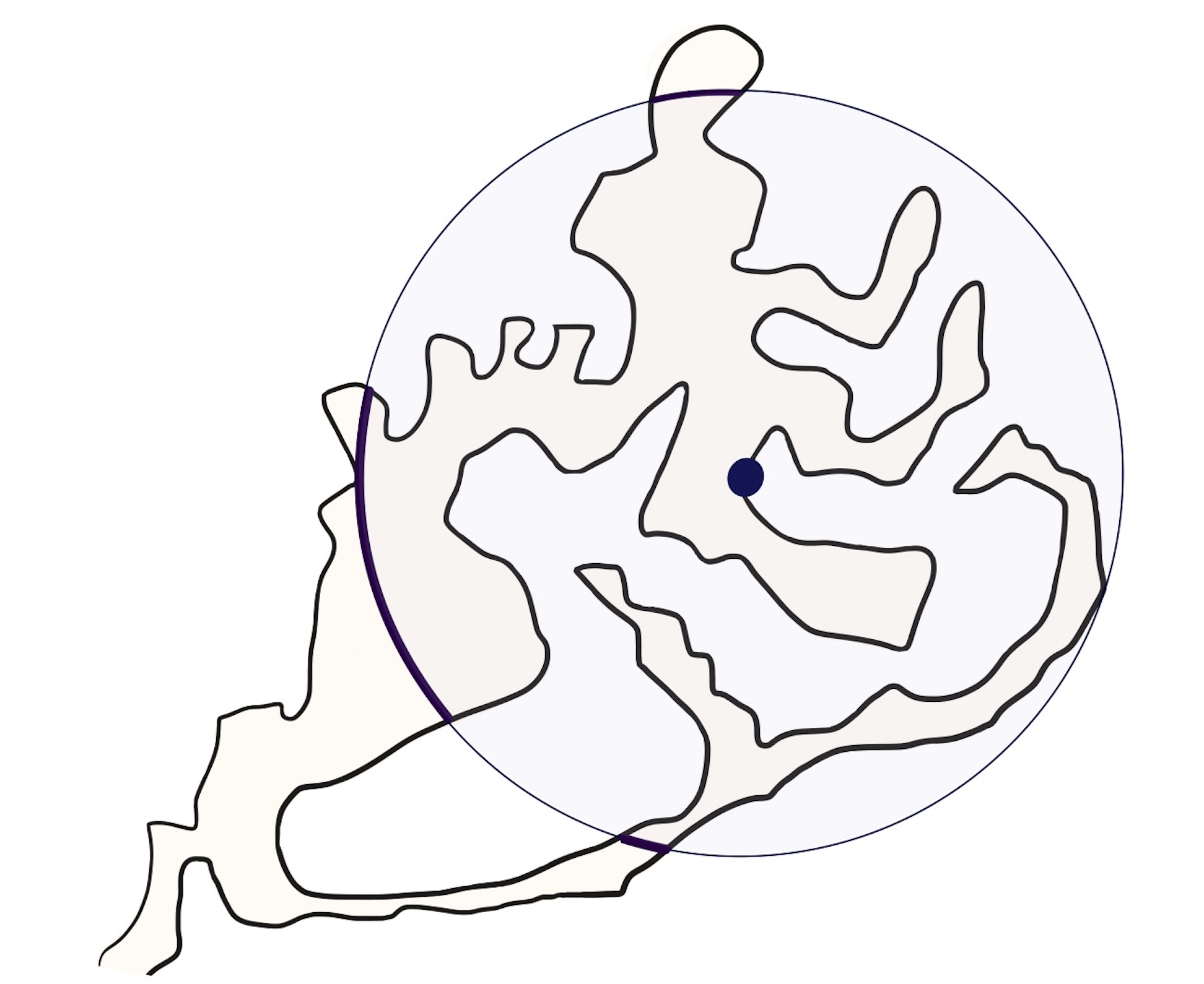
Figure 2: Figure pertaining to the proof that Jordan curves are weakly Ahlfors regular (Lemma 3.1). The union $\mathcal{C}$ of circular arcs intersecting the Jordan domain $\mathcal{G}$ is shown in purple, and the domains enclosed by $(\Gamma\cap D)\cup\mathcal{C}$ are lightly shaded.

Proof.

Denote by $\mathcal{G}$ the Jordan domain enclosed by $\Gamma$ and fix an open disk $D$. We first assume that $\Gamma$ is analytic, which implies that either $\Gamma=\partial D$, or it has finitely many intersections with $\partial D$. Indeed, after a translation and a rescaling, we may assume that $D$ is the unit disk. If $\phi:{\mathbb{D}}\to\mathcal{G}$ is a conformal map, it extends conformally past the boundary, and $f$ is real-analytic on the circle. If $\#(\Gamma\cap\partial D)$ were infinite, then the zeros of the real-analytic function $f(s)\overset{{\sf def}}{=}|\phi(e^{{\rm i}s})|^{2}-1$ would have an accumulation point, which implies that $f(s)=0$, so $\Gamma$ coincides with a circle. Hence, $\mathcal{G}\cap D$ is a finite union of Jordan domains with piecewise analytic boundaries. Moreover, $\mathcal{C}\overset{{\sf def}}{=}\overline{\mathcal{G}\cap\partial D}$ is a disjoint finite union of circular arcs. If these are given the positive orientation, the domain $\mathcal{G}$ always remains on the left-hand side as we traverse $\mathcal{C}$, and we find that the curve

$$\left(\Gamma\cap D\right)\cup\mathcal{C}$$

is a finite union of piecewise smooth Jordan curves, each of which bounds a connected component of $\mathcal{G}\cap D$; see Figure 2. Cauchy’s theorem then gives that

$$\int_{\Gamma\cap D}{{\rm d}z}=-\int_{\mathcal{C}}{{\rm d}z},$$ (3.2)

and we clearly have that

$$\left|\int_{\mathcal{C}}{{\rm d}z}\right|\leq\int_{\mathcal{C}}|{\rm d}z|=|\partial D|.$$ (3.3)

Hence, the proof is complete for analytic curves.

For a general rectifiable Jordan curve $\Gamma$, we argue by approximation. By Carathéodory’s theorem, there exists a conformal mapping $\phi$ of ${\mathbb{D}}$ onto $\mathcal{G}$, such that $\phi$ extends to a homeomorphism $\phi:\overline{{\mathbb{D}}}\to\overline{\mathcal{G}}$. We obtain the desired approximation by taking $\Gamma_{t}$ to be the curve parametrized by $\phi(te^{{\rm i}s})$, $s\in[0,2\pi)$, for $0<t<1$ and letting $t\to 1$. Since $\Gamma$ is rectifiable, a theorem of Riesz and Privalov (see [20, 6.8]) asserts that the derivative $\phi^{\prime}(z)$ belongs to the Hardy space $H^{1}({\mathbb{T}})$. In particular, the radial limit $\phi^{\prime}=\lim_{t\to 1}\phi^{\prime}_{t}$ exists a.e. on ${\mathbb{T}}$, and $\phi_{t}^{\prime}\to\phi^{\prime}$ in $L^{1}({\mathbb{T}})$. Since $\phi(e^{{\rm i}s})$ supplies an absolutely continuous parametrization of $\Gamma$, the quantity of interest may be expressed as

$$\int_{\Gamma\cap D}{\rm d}z=\int_{0}^{2\pi}{1\hskip-2.5pt{\rm l}}_{D}\big{(}\phi(e^{{\rm i}s})\big{)}\partial_{s}\phi(e^{{\rm i}s})\,{\rm d}s=\int_{0}^{2\pi}{1\hskip-2.5pt{\rm l}}_{D}\big{(}\phi(e^{{\rm i}s})\big{)}{\rm i}e^{{\rm i}s}\phi^{\prime}(e^{{\rm i}s})\,{\rm d}s.$$

Next, note that ${1\hskip-2.5pt{\rm l}}_{D}\circ\phi_{t}\to{1\hskip-2.5pt{\rm l}}_{D}\circ\phi$ holds everywhere on the circle. Indeed, since $D$ is open, any point $\phi(e^{{\rm i}s})\in D$ has a neighborhood $V\subset D$. But since $\phi_{t}(e^{{\rm i}s})\to\phi(e^{{\rm i}s})$ for any $s$, we have $\phi_{t}(e^{{\rm i}s})\in V$ for $t$ sufficiently close to $1$.

As a consequence of these properties of the approximating parametrization we find that for any fixed disk $D$, we have

$$\lim_{t\to 1}\int_{0}^{2\pi}{1\hskip-2.5pt{\rm l}}_{D}\big{(}\phi_{t}(e^{{\rm i}s})\big{)}{\rm i}e^{{\rm i}s}\phi_{t}^{\prime}(e^{{\rm i}s})\,{\rm d}s=\int_{0}^{2\pi}{1\hskip-2.5pt{\rm l}}_{D}\big{(}\phi(e^{{\rm i}s})\big{)}{\rm i}e^{{\rm i}s}\phi^{\prime}(e^{{\rm i}s})\,{\rm d}s,$$

or, in other words,

$$\lim_{t\to 1}\int_{\Gamma_{t}\cap D}{\rm d}z=\int_{\Gamma\cap D}{\rm d}z.$$

Hence, for any given disk $D$ and any fixed $\varepsilon>0$, we let $t$ be sufficiently close to $1$ so that

$$\left|\int_{\Gamma\cap D}{\rm d}z-\int_{\Gamma_{t}\cap D}{\rm d}z\right|\leq\varepsilon|\partial D|.$$

But since $\Gamma_{t}$ is analytic, it follows from (3.2) and (3.3) and the reverse triangle inequality that

$$\left|\int_{\Gamma\cap D}{\rm d}z\right|\leq(1+\varepsilon)|\partial D|.$$

Since $\varepsilon>0$ was arbitrary, the claim follows. ∎

If a rectifiable Jordan arc $\Gamma$ can be completed to a rectifiable Jordan curve by appending a weakly Ahlfors regular Jordan arc, then $\Gamma$ is also weakly Ahlfors regular; cf. Figure 3. The existence of such an arc would be guaranteed if, e.g., $\Gamma$ does not wind too wildly near any of its endpoints. Hence, at least for rectifiable Jordan arcs, only the behavior near the end-points matter for weak regularity.

3.2 The density of $\nu_{\Gamma}$

We denote by $\gamma:I\to\Gamma$ the arc-length parametrization of $\Gamma$, and introduce the (“net tangent”) function

$$\tau(x)=\tau_{\Gamma}(x)\overset{{\sf def}}{=}\sum_{t\in\gamma^{-1}(x)}\gamma^{\prime}(t).$$ (3.4)

Let $\nu_{\Gamma}$ be the complex-valued measure given by the integration current over $\Gamma$. That is,

$$\int h\,{\rm d}\nu_{\Gamma}=\int_{\Gamma}h(z)\,{\rm d}z=\int_{I}h(\gamma(t))\,\gamma^{\prime}(t)\,{\rm}{\rm d}t.$$ (3.5)

Then, for any Borel set $B$, $\displaystyle\nu_{\Gamma}(B)=\int_{\Gamma\cap B}{\rm d}z$.

Recall that $\mathcal{H}^{1}$ is the one-dimensional Hausdorff measure on ${\mathbb{C}}$.

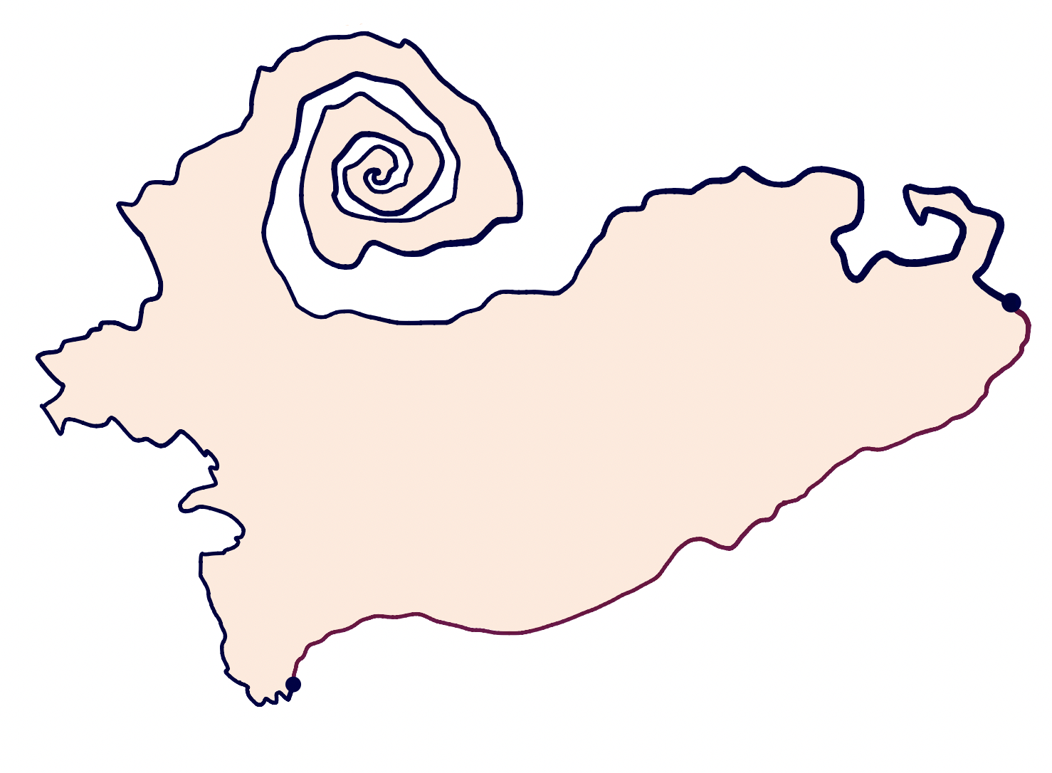
Figure 3: A Jordan arc $\Gamma$ (black) which can be completed to a Jordan curve by appending a weakly Ahlfors regular arc (red), implying that $\Gamma$ is weakly Ahlfors; cf. Lemma 3.1.

Lemma 3.2.

Assume that $\Gamma$ is a weakly Ahlfors regular rectifiable curve. Then for $\mathcal{H}^{1}$-a.e. $x$, it holds that

$$\lim_{\varepsilon\to 0}\frac{1}{\varepsilon}\int_{0}^{\varepsilon}\frac{\nu_{\Gamma}\left({\mathbb{D}}(x,r)\right)}{2r}{\rm d}r=\tau(x).$$

Proof.

From (3.5), it is evident that $\nu_{\Gamma}$ is absolutely continuous with respect to arc-length measure on $\Gamma$, which in turn is absolutely continuous with respect to $\mathcal{H}^{1}\big{|}_{\Gamma}$. In fact, by applying the change of variables formula in [5, Theorem 3.9] to the functions $g=(h\circ\gamma)\,\gamma^{\prime}$ and $f=\gamma$ (so that the Jacobian satisfies $Jf=1$ a.e.), we find that

$$\int_{I}h(\gamma(t))\gamma^{\prime}(t)\,{\rm d}t=\int_{\Gamma}h(x)\left(\sum_{t\in\gamma^{-1}(x)}\gamma^{\prime}(t)\right){\rm d}\mathcal{H}^{1}(x)=\int_{\Gamma}h(x)\tau(x)\,{\rm d}\mathcal{H}^{1}(x),$$

so that ${\rm d}\nu_{\Gamma}(x)=\tau(x)\,{\rm d}\mathcal{H}^{1}\big{|}_{\Gamma}(x)$. In view of the upper bound

$$\int_{\Gamma}|\tau(x)|\,{\rm d}\mathcal{H}^{1}(x) \leq\int_{\Gamma}\#\big{\{}t\in\gamma^{-1}(x)\big{\}}{\rm d}\mathcal{H}^{1}(x)$$

$$=\int_{I}|\gamma^{\prime}(t)|\,{\rm d}t=|\Gamma|,$$

and of the rectifiability of $\Gamma$, we have $\tau\in L^{1}(\mathcal{H}^{1}|_{\Gamma})$.

We next claim that

$$\frac{\mathcal{H}^{1}|_{\Gamma}({\mathbb{D}}(x,r))}{2r}\xrightarrow{r\to 0}1.$$ (3.6)

Indeed, the upper bound follows from the density bound [16, Theorem 6.2] for general rectifiable sets, and the lower bound is a consequence of the fact that $\Gamma$ has a tangent at $\mathcal{H}^{1}$-a.e. $x\in\Gamma$.

Since $\mathcal{H}^{1}|_{\Gamma}$ is a Borel regular measure (see [16, p. 57]), we may apply the Lebesgue-Besicovitch differentiation theorem ([5, Theorem 1.32]) along with (3.6) to obtain

$$\lim_{r\to 0}\frac{\nu_{\Gamma}({\mathbb{D}}(x,r))}{2r}=\lim_{r\to 0}\frac{1}{\mathcal{H}^{1}|_{\Gamma}({\mathbb{D}}(x,r))}\int_{\Gamma\cap{\mathbb{D}}(x,r)}\tau(x){\rm d}\mathcal{H}^{1}(x)\cdot\frac{\mathcal{H}^{1}|_{\Gamma}({\mathbb{D}}(x,r))}{2r}=\tau(x)$$ (3.7)

for $\mathcal{H}^{1}$-a.e. $x\in{\mathbb{C}}$.

Observe next that

$$\frac{1}{\varepsilon}\int_{0}^{\varepsilon}\frac{\nu_{\Gamma}\left({\mathbb{D}}(x,r)\right)}{2r}{\rm d}r=\int_{0}^{1}\frac{\nu_{\Gamma}\left({\mathbb{D}}(x,\varepsilon t)\right)}{2\varepsilon t}{\rm d}t,$$

and in view of the weak Ahlfors regularity of $\Gamma$, the integrand on the right-hand side is bounded above by $1$. Hence, the pointwise convergence (3.7) and the bounded convergence theorem together give that

$$\lim_{\varepsilon\to 0}\frac{1}{\varepsilon}\int_{0}^{\varepsilon}\frac{\nu_{\Gamma}\left({\mathbb{D}}(x,r)\right)}{2r}{\rm d}r=\int_{0}^{1}\tau(x){\rm d}t=\tau(x)$$

for $\mathcal{H}^{1}$-a.e. $x\in{\mathbb{C}}$. This completes the proof. ∎

Remark 3.3.

In view of Lemma 3.2, the net tangent $\tau_{\Gamma}$ of the weakly Ahlfors regular rectifiable curve $\Gamma$ (i.e., the density of ${{\rm d}z}$ along $\Gamma$ with respect to Hausdorff measure $\mathcal{H}^{1}$) belongs to $L^{\infty}({\mathbb{C}},{\rm d}\mathcal{H}^{1})$.

Furthermore, since $\Gamma_{1}$ and $\Gamma_{2}$ are assumed to be rectifiable, the angle between the tangents is either $0$ or $\pi$ at $\mathcal{H}^{1}$-a.e. point where the curves intersect. Indeed, the set of points in the intersection for which neither of the curves have a unimodular tangent has $\mathcal{H}^{1}$-measure $0$. Furthermore, for any point in $\Gamma_{1}\cap\Gamma_{2}$ where both curves have unimodular tangent and the angle of intersection is not $0$ or $\pi$, there exists a punctured neighborhood where the curves do not intersect. Therefore, the set of such points is at most countable.

Combining both observations with the definition (1.8) of $\mathcal{L}(\Gamma_{1},\Gamma_{2})$ and formula (3.4) for the net tangent $\tau_{\Lambda}$, we arrive at the formula

$$\mathcal{L}(\Gamma_{1},\Gamma_{2}) =\int_{{\mathbb{C}}}\bigg{(}\sum_{s\in\gamma_{1}^{-1}(z),\;t\in\gamma_{2}^{-1}(z)}\operatorname{Re}\big{(}\gamma_{1}^{\prime}(s)\,\overline{\gamma_{2}^{\prime}(t)}\big{)}\bigg{)}\,{\rm d}\mathcal{H}^{1}(z)$$ (3.8)

$$=\int_{{\mathbb{C}}}\bigg{(}\sum_{s\in\gamma_{1}^{-1}(z),\;t\in\gamma_{2}^{-1}(z)}\gamma_{1}^{\prime}(s)\,\overline{\gamma_{2}^{\prime}(t)}\bigg{)}\,{\rm d}\mathcal{H}^{1}(z)$$ (3.9)

$$=\int_{\Gamma_{1}\cap\Gamma_{2}}\tau_{\Gamma_{1}}(x)\overline{\tau_{\Gamma_{2}}(x)}\,{\rm d}\mathcal{H}^{1}(x)\,.$$ (3.10)

In particular, we see that the signed length $\mathcal{L}(\Gamma_{1},\Gamma_{2})$ is finite whenever $\Gamma_{1}$ and $\Gamma_{2}$ are weakly Ahlfors regular rectifiable curves.

4 The covariance structure of $\mathcal{E}_{\Lambda}(\Gamma)$

The purpose of this section is to establish the basic formula (1.13) for the covariance of the action of $V_{\Lambda}$ along two weakly Ahlfors regular rectifiable curves. The starting point is the following result taken from Proposition 5.9 and Remark 5.11 in Part I.

Lemma 4.1.

Assume that $(1+t^{2})k_{\Lambda}\in L^{1}({\mathbb{R}}_{\geq 0},{\rm d}t)$. Then for $\varphi,\psi\in\mathcal{S}$, we have

$${\sf Cov}\left[V_{\Lambda}(\varphi),V_{\Lambda}(\psi)\right]=\iint_{{\mathbb{C}}\times{\mathbb{C}}}\varphi(x)\overline{\psi(y)}K(|x-y|)\,{\rm d}m(x)\,{\rm d}m(y),$$ (4.1)

where the kernel $K=K_{V_{\Lambda}}$ (the two-point function for $V_{\Lambda}$) is given by

$$K(z)=-4\pi^{2}\int_{0}^{\infty}\log_{+}\left(\frac{r}{|z|}\right)k_{\Lambda}(r)\,r\,{\rm d}r,\qquad z\in{\mathbb{C}}\setminus\{0\}.$$

Juxtaposing (4.1) with the formula for the covariance on the Fourier side:

$${\sf Cov}\left[V_{\Lambda}(\varphi),V_{\Lambda}(\psi)\right]=\int_{{\mathbb{C}}}\widehat{\varphi}(\xi)\,\overline{\widehat{\psi}(\xi)}\,\frac{{\rm d}\rho_{\Lambda}(\xi)}{|\xi|^{2}}$$ (4.2)

(see Theorem 5.8, Part I), we conclude that

$$\widehat{K}(\xi)=|\xi|^{-2}h_{\Lambda}\,,$$ (4.3)

where $h_{\Lambda}$ is the (radial) density of $\rho_{\Lambda}$. The Fourier transform in (4.3) should be understood in the sense of distributions, or alternatively in the sense of Fourier transform acting on $L^{2}({\mathbb{C}},m)$ functions.

For the remainder of this section, we will work in somewhat greater generally with observables $\mu(V_{\Lambda})$, where $\mu$ is an admissible measure (recall Definition 2.1 above). In order to show that the variance of $\mu(V_{\Lambda})$ is well defined, we will approximate $\mu$ by $\mu_{\varepsilon}=\mu*\phi_{\varepsilon}$, where $\phi_{\varepsilon}(z)$ are the Gaussians from (2.2).

Lemma 4.2.

Assume that $\mu$ and $\nu$ are admissible complex-valued measures. Then we have $\mu(V_{\Lambda}),\nu(V_{\Lambda})\in L^{2}(\Omega,\mathbb{P})$, and

$${\sf Cov}\left[\int_{{\mathbb{C}}}V_{\Lambda}(z)\,{{\rm d}\mu}(z),\int_{{\mathbb{C}}}V_{\Lambda}(z)\,{\rm d}\nu(z)\right]=\lim_{\varepsilon\to 0}\iint_{{\mathbb{C}}\times{\mathbb{C}}}K(|x-y|)\,{{\rm d}\mu}_{\varepsilon}(x)\,{\rm d}\bar{\nu}_{\varepsilon}(y).$$

Proof.

It will suffice to show that $\mu(V_{\Lambda})=\int V_{\Lambda}{{\rm d}\mu}\in L^{2}(\Omega,\mathbb{P})$ and that

$${\sf Var}\left[\mu(V_{\Lambda})\right]=\lim_{\varepsilon\to 0}\iint_{{\mathbb{C}}\times{\mathbb{C}}}K(|x-y|)\,{\rm d}\mu_{\varepsilon}(x)\,{\rm d}\bar{\mu}_{\varepsilon}(y).$$

Since $\mu_{\varepsilon}$ is absolutely continuous with a density in $\mathcal{S}$, by (4.3) we have

$${\sf Var}\left[\mu_{\varepsilon}(V_{\Lambda})\right]=\int_{{\mathbb{C}}}|\widehat{\mu}_{\varepsilon}(\xi)|^{2}\,\frac{{\rm d}\rho_{\Lambda}(\xi)}{|\xi|^{2}}=\int_{{\mathbb{C}}}e^{-\varepsilon^{2}|\xi|^{2}}|\widehat{\mu}(\xi)|^{2}\,\frac{{\rm d}\rho_{\Lambda}(\xi)}{|\xi|^{2}}.$$

Notice that the integrand is monotonically increasing as $\varepsilon$ decreases to $0$, so it will be sufficient to establish that

$$\sup_{\varepsilon>0}\int_{{\mathbb{C}}}e^{-\varepsilon^{2}|\xi|^{2}}|\widehat{\mu}(\xi)|^{2}\,\frac{{\rm d}\rho_{\Lambda}(\xi)}{|\xi|^{2}}<\infty.$$ (4.4)

Indeed, it will then follow from monotone convergence that ${\sf Var}\left[\mu_{\varepsilon}(V_{\Lambda})\right]$ converges to $\lVert\widehat{\mu}\rVert_{L^{2}(|\xi|^{-2}\rho_{\Lambda})}^{2}$ as $\varepsilon\to 0$, which implies that

$$\lVert\widehat{\mu}_{\varepsilon}-\widehat{\mu}_{\delta}\rVert_{L^{2}({\mathbb{C}},|\xi|^{-2}\rho_{\Lambda})}^{2}=\int_{{\mathbb{C}}}\Big{(}e^{-\varepsilon^{2}|\xi|^{2}}+e^{-\delta^{2}|\xi|^{2}}-2e^{-\frac{\varepsilon^{2}+\delta^{2}}{2}|\xi|^{2}}\Big{)}|\widehat{\mu}(\xi)|^{2}\,\frac{{\rm d}\rho_{\Lambda}(\xi)}{|\xi|^{2}}\to 0$$

as $\varepsilon,\delta\to 0$. Hence, we see that $\displaystyle\mu(V_{\Lambda})=\lim_{\varepsilon\to 0}\,\mu_{\varepsilon}(V_{\Lambda})$ in $L^{2}(\Omega,\mathbb{P})$, and the variance may be expressed as

$${\sf Var}[\mu(V_{\Lambda})]=\lim_{\varepsilon\to 0}\iint_{{\mathbb{C}}\times{\mathbb{C}}}K(|x-y|)\,{{\rm d}\mu}_{\varepsilon}(x)\,{\rm d}\bar{\mu}_{\varepsilon}(y).$$

In order to see why (4.4) holds, notice that by Lemma 4.1 we have

$${\sf Var}\left[\mu_{\varepsilon}(V_{\Lambda})\right] =\iint_{{\mathbb{C}}\times{\mathbb{C}}}K(|x-y|)\,{{\rm d}\mu}_{\varepsilon}(x)\,{\rm d}\bar{\mu}_{\varepsilon}(y)$$ (4.5)

$$=-4\pi^{2}\iint_{{\mathbb{C}}\times{\mathbb{C}}}\left(\int_{0}^{\infty}\log_{+}\frac{t}{|x-y|}k_{\Lambda}(t)\,t\,{\rm d}t\right){{\rm d}\mu}_{\varepsilon}(x)\,{\rm d}\bar{\mu}_{\varepsilon}(y).$$ (4.6)

Note that the measure $|\mu_{\varepsilon}|$ is absolutely continuous with density in $\mathcal{S}$, so we may integrate against $|\mu_{\varepsilon}|\times|\mu_{\varepsilon}|$ to get

$$\iint_{{\mathbb{C}}\times{\mathbb{C}}}\int_{0}^{\infty}\log_{+}\frac{t}{|x-y|}|k_{\Lambda}(t)|\,t\,{\rm d}|\mu_{\varepsilon}|(x)\,{\rm d}|\mu_{\varepsilon}|(y)\,{\rm dt}\\ \leq\iint_{{\mathbb{C}}\times{\mathbb{C}}}\int_{0}^{\infty}\left(\big{|}\log|x-y|\big{|}+\big{|}\log t\big{|}\right)|k_{\Lambda}(t)|\,t\,{\rm d}|\mu_{\varepsilon}|(x)\,{\rm d}|\mu_{\varepsilon}|(y)\,{\rm dt}\\ \lesssim_{\varepsilon}\int_{0}^{\infty}\big{(}1+|\log t|\big{)}|k_{\Lambda}(t)|\,t\,{\rm d}t<\infty.$$ (4.7)

We may thus apply Fubini’s theorem to the right-hand side of (4.5) to get

$${\sf Var}\left[\mu_{\varepsilon}(V_{\Lambda})\right]=-4\pi^{2}\int_{{\mathbb{C}}}\int_{0}^{\infty}t^{2}k_{\Lambda}(t)I_{\varepsilon}(t,x)\,{\rm d}t\,{\rm d}\mu_{\varepsilon}(x),$$

where

$$I_{\varepsilon}(t,x)=\frac{1}{t}\int_{\mathbb{C}}\log_{+}\frac{t}{|x-y|}\,{\rm d}\bar{\mu}_{\varepsilon}(y)=\frac{1}{t}\int_{0}^{\infty}\bar{\mu}_{\varepsilon}\left({\mathbb{D}}(x,te^{-s})\right)\,{\rm d}s,$$

the last equality being a consequence of the “layer cake formula”; that is, integration with respect to the distribution function. Hence, by the triangle inequality, we get that

$${\sf Var}\left[\mu_{\varepsilon}(V_{\Lambda})\right]\leq 4\pi^{2}\int_{{\mathbb{C}}}\int_{0}^{\infty}t^{2}\,|k_{\Lambda}(t)|\,|I_{\varepsilon}(t,x)|\,{\rm d}t\,{\rm d}|\mu_{\varepsilon}|(x).$$

By Claim 2.2, the measure $\mu_{\varepsilon}$ is admissible, with admissibility constant independent of $\varepsilon$. Therefore,

$$|I_{\varepsilon}(t,x)|\leq\frac{1}{t}\int_{0}^{t}\frac{|\mu_{\varepsilon}\left({\mathbb{D}}(x,r)\right)|}{r}{\rm d}r\leq C_{\mu},$$

and, as a consequence,

$${\sf Var}\left[\mu_{\varepsilon}(V_{\Lambda})\right]\leq C_{\mu}|\mu_{\varepsilon}|({\mathbb{C}})\int_{0}^{\infty}t^{2}\,|k_{\Lambda}(t)|\,{\rm d}t,$$

which is readily seen to be bounded above independently of $\varepsilon$ by use of the trivial bound $|\mu*\phi_{\varepsilon}|({\mathbb{C}})\leq|\mu|({\mathbb{C}})\int_{\mathbb{C}}\phi_{\varepsilon}(z){\rm d}m(z)=|\mu|({\mathbb{C}})$. ∎

Since in the end we prefer to think in terms of the principal value integral, we should check that both regularizations of the integral $\displaystyle{\iint_{{\mathbb{C}}\times{\mathbb{C}}}K(|x-y|)\,{\rm d}\mu(x)\,{\rm d}\bar{\mu}(y)}$ give the same result.

Lemma 4.3.

For any two admissible measures $\mu$ and $\nu$, we have that

$$\lim_{\varepsilon\to 0}\iint_{{\mathbb{C}}\times{\mathbb{C}}}K(|x-y|)\,{{\rm d}\mu}_{\varepsilon}(x)\,{\rm d}\bar{\nu}_{\varepsilon}(y) =\lim_{\varepsilon\to 0}\iint_{{\mathbb{C}}\times{\mathbb{C}}}{1\hskip-2.5pt{\rm l}}_{\{|x-y|>\varepsilon\}}K(|x-y|)\,{\rm d}\mu(x)\,{\rm d}\bar{\nu}(y)$$

$$\overset{{\sf def}}{=}{\sf p.v.}\iint_{{\mathbb{C}}\times{\mathbb{C}}}K(|x-y|)\,{{\rm d}\mu}(x)\,{\rm d}\bar{\nu}(y).$$

Proof.

Again, by polarization, it suffices to check the condition for $\mu=\nu$. Recall that the convolution of two centered Gaussians is again a centered Gaussian;

$$\phi_{\varepsilon}*\phi_{\varepsilon}=\phi_{\sqrt{2}\varepsilon}.$$ (4.8)

Thinking of $K$ as a function in ${\mathbb{C}}$ by the identification $K(z)=K(|z|)$, we rewrite the regularized variance as

$$\iint_{{\mathbb{C}}\times{\mathbb{C}}}K(|x-y|)\,{{\rm d}\mu}_{\varepsilon}(x)\,{\rm d}\bar{\mu}_{\varepsilon}(y) =\int_{\mathbb{C}}[K*\phi_{\varepsilon}*\bar{\mu}]\,[\phi_{\varepsilon}*\mu]\,{\rm d}m$$ (4.9)

$$=\int_{\mathbb{C}}[K*\phi_{\varepsilon}*\bar{\mu}]*\phi_{\varepsilon}\,{{\rm d}\mu}$$ (4.10)

where we have used the general distributional identity

$$\left(f,g*h\right)=\left(f*g,h\right)$$

applied to $f=K*\phi_{\varepsilon}$, $g=\phi_{\varepsilon}$ and $h=\mu$ to arrive at the last equality. Using the associativity of convolution along with the identity (4.8), we recognize this as

$$\int_{\mathbb{C}}[K*\phi_{\varepsilon}*\bar{\mu}]*\phi_{\varepsilon}\,{{\rm d}\mu}=\int_{{\mathbb{C}}}\left(\int_{{\mathbb{C}}}K(|x-y|)\,{\rm d}\bar{\mu}_{\sqrt{2}\varepsilon}(y)\right){{\rm d}\mu}(x).$$

The quantity of interest is thus

$$\int_{{\mathbb{C}}}\bigg{(}\int_{{\mathbb{C}}}K(|x-y|)\,{\rm d}\bar{\mu}_{\sqrt{2}\varepsilon}(y)-\int_{|x-y|>\varepsilon}K(|x-y|)\,{\rm d}\bar{\mu}(y)\bigg{)}{{\rm d}\mu}(x)\\ =-4\pi^{2}\int_{{\mathbb{C}}}\int_{0}^{\infty}k_{\Lambda}(t)t^{2}I^{\Delta}_{\varepsilon}(t,x)\,{\rm d}t\,{\rm d}\mu_{\varepsilon}(x)$$ (4.11)

where

$$I^{\Delta}_{\varepsilon}(t,x) =\frac{1}{t}\int_{0}^{\infty}\left[\mu_{\sqrt{2}\varepsilon}\left({\mathbb{D}}(x,te^{-s})\right)-\mu\left({\mathbb{D}}(x,te^{-s})\setminus{\mathbb{D}}(x,\varepsilon)\right)\right]{\rm d}s$$ (4.12)

$$=\frac{1}{t}\int_{0}^{t}\left(\frac{\mu_{\sqrt{2}\varepsilon}\left({\mathbb{D}}(x,r)\right)}{r}-\frac{\mu\left({\mathbb{D}}(x,r)\setminus{\mathbb{D}}(x,\varepsilon)\right)}{r}\right){\rm d}r.$$ (4.13)

By the admissibility assumption and by the fact that convolution preserves weak Ahlfors regularity (Claim 2.2), the integrand on the right-hand side is uniformly bounded, as

$$\bigg{|}\frac{\mu_{\sqrt{2}\varepsilon}\left({\mathbb{D}}(x,r)\right)}{r}-\frac{\mu\left({\mathbb{D}}(x,r)\setminus{\mathbb{D}}(x,\varepsilon)\right)}{r}\bigg{|}\leq\frac{|\mu_{\sqrt{2}\varepsilon}({\mathbb{D}}(x,r))|}{r}+\frac{|\mu({\mathbb{D}}(x,r))|}{r}\leq 2\,C_{\mu}\,.$$

Therefore, we can apply the bounded convergence theorem for each fixed $t>0$ and get

$$\lim_{\varepsilon\to 0}I^{\Delta}_{\varepsilon}(t,x)=0$$

for $\mathcal{H}^{1}$-a.e. $x$. Hence, in view of the condition that $t^{2}k_{\Lambda}(t)\in L^{1}({\mathbb{R}}_{\geq 0},{\rm d}t)$, the claim follows from the dominated convergence theorem. ∎

5 Proof of the main results

5.1 The asymptotic covariance structure of the electric action

Recall that Theorem 1.3 asserts that if the two-point function $k_{\Lambda}$ is radial and satisfies $(1+t^{2})k_{\Lambda}(t)\in L^{1}({\mathbb{R}}_{\geq 0},{\rm d}t)$, then for any weakly Ahlfors regular rectifiable curves $\Gamma_{1}$ and $\Gamma_{2}$ we have

$${\sf Cov}\left[\int_{R\Gamma_{1}}V_{\Lambda}(z)\,{\rm d}z,\int_{R\Gamma_{2}}V_{\Lambda}(z)\,{\rm d}z\right]=R\left(C_{\Lambda}+o(1)\right)\mathcal{L}(\Gamma_{1},\Gamma_{2})$$

as $R\to\infty$, where $\displaystyle{C_{\Lambda}=-8\pi^{2}\int_{0}^{\infty}k_{\Lambda}(t)\,t^{2}\,{\rm d}t}$.

Proof of Theorem 1.3.

We will show that for any two admissible measures $\mu$ and $\nu$ such that the limit

$$\tau_{\nu}(x)\overset{{\sf def}}{=}\lim_{\varepsilon\to 0}\frac{1}{\varepsilon}\int_{0}^{\varepsilon}\frac{\nu({\mathbb{D}}(x,r))}{2r}{\rm d}r$$ (5.1)

exists $\mathcal{H}^{1}$-a.e., we have

$${\sf Cov}\left[\int_{{\mathbb{C}}}V_{\Lambda}(Rz)\,{{\rm d}\mu}(z),\int_{{\mathbb{C}}}V_{\Lambda}(Rz)\,{\rm d}\nu(z)\right]=\left(C_{\Lambda}+o(1)\right)\,R^{-1}\int_{{\mathbb{C}}}\overline{\tau_{\nu}(z)}\,{{\rm d}\mu}(z).$$ (5.2)

Theorem 1.3 will follow by combining (5.2) with Lemma 3.2, which states that (5.1) holds for the complex-valued measure $\nu_{\Gamma}$, which was defined by $\nu_{\Gamma}(f)=\int_{\Gamma}f\,{\rm d}z$. This measure is clearly admissible, since $\Gamma$ is assumed to be weakly Ahlfors regular. We note that

$$\int_{\Gamma_{1}\cap\Gamma_{2}}\overline{\tau_{\Gamma_{2}}(x)}\,{\rm d}\nu_{\Gamma_{1}}(x)=\int_{\Gamma_{1}\cap\Gamma_{2}}\tau_{\Gamma_{1}}(x)\,\overline{\tau_{\Gamma_{2}}(x)}\,{\rm d}\mathcal{H}^{1}(x)=\mathcal{L}(\Gamma_{1},\Gamma_{2}),$$

see Remark 3.3.

Putting together the two formulas from Lemma 4.2 and Lemma 4.3 for the regularized covariance, we have

$${\sf Cov}\left[\int_{{\mathbb{C}}}V_{\Lambda}(Rz)\,{{\rm d}\mu}(z),\int_{{\mathbb{C}}}V_{\Lambda}(Rz)\,{\rm d}\nu(z)\right] ={\sf p.v.}\iint_{{\mathbb{C}}\times{\mathbb{C}}}K(R|x-y|)\,{{\rm d}\mu}(x)\,{\rm d}\bar{\nu}(y)$$ (5.3)

$$=\lim_{\varepsilon\to 0}\iint_{{\mathbb{C}}\times{\mathbb{C}}}{1\hskip-2.5pt{\rm l}}_{\{|x-y|>\varepsilon\}}K(R|x-y|)\,{{\rm d}\mu}(x)\,{\rm d}\bar{\nu}(y).$$ (5.4)

For any $\varepsilon>0$, we may write the truncated covariance integral as

$$\iint_{{\mathbb{C}}\times{\mathbb{C}}}{1\hskip-2.5pt{\rm l}}_{\{|x-y|>\varepsilon\}}K(R|x-y|)\,{{\rm d}\mu}(x)\,{\rm d}\bar{\nu}(y)\\ =-4\pi^{2}\int_{{\mathbb{C}}}\int_{|x-y|>\varepsilon}\int_{0}^{\infty}\log_{+}\frac{t/R}{|x-y|}k_{\Lambda}(t)\,t\,{\rm d}t\,{{\rm d}\mu}(x)\,{\rm d}\bar{\nu}(y).$$ (5.5)

This integral is absolutely convergent, and an application of Fubini’s theorem gives that

$$\iint_{{\mathbb{C}}\times{\mathbb{C}}}{1\hskip-2.5pt{\rm l}}_{\{|x-y|>\varepsilon\}}K(R|x-y|)\,{{\rm d}\mu}(x)\,{\rm d}\bar{\nu}(y)\\ =\frac{1}{R}\int_{{\mathbb{C}}}I_{R,\varepsilon}(x)\,{{\rm d}\mu}(x)$$

where

$$I_{R,\varepsilon}(x) =-4\pi^{2}\int_{0}^{\infty}k_{\Lambda}(t)\,t^{2}\left(\frac{R}{t}\int_{|x-y|>\varepsilon}\log_{+}\frac{t/R}{|x-y|}\,{\rm d}\bar{\nu}(y)\right)\,{\rm d}t$$ (5.6)

$$\overset{{\sf def}}{=}-4\pi^{2}\int_{0}^{\infty}k_{\Lambda}(t)\,t^{2}J_{R,t,\varepsilon}(x){\rm d}t.$$ (5.7)

Integrating with respect to the distribution function, we arrive at

$$J_{R,t,\varepsilon}(x) =\frac{R}{t}\int_{|x-y|>\varepsilon}\log_{+}\frac{t/R}{|x-y|}{\rm d}\bar{\nu}(y)$$ (5.8)

$$=\frac{1}{t/R}\int_{0}^{\infty}\bar{\nu}\left(\left\{y:\varepsilon<|x-y|<\frac{t}{R}e^{-s}\right\}\right){\rm d}s$$ (5.9)

$$=\frac{1}{t/R}\int_{\varepsilon}^{t/R}\frac{\bar{\nu}\left({\mathbb{D}}(x,r)\setminus{\mathbb{D}}(x,\varepsilon)\right)}{r}{\rm d}r.$$ (5.10)

By the definition of admissible measures, we have

$$|J_{R,t,\varepsilon}(x)|\leq C$$

uniformly in $x,R$ $t$ and $\varepsilon$. What is more, the existence of $\displaystyle\lim_{\varepsilon\to 0}J_{R,t,\varepsilon}(x)=J_{R,t,0}(x)$ for all $x$ follows from admissibility, while the assumption (5.1) together with admissibility of $\nu$ ensure that for any fixed $t>0$, we have

$$J_{R,t,0}(x)=\frac{1}{t/R}\int_{0}^{t/R}\frac{\bar{\nu}\left({\mathbb{D}}(x,r)\right)}{r}{\rm d}r\xrightarrow{R\to\infty}2\overline{\tau_{\nu}(x)}$$

for $\mathcal{H}^{1}$-a.e. $x\in{\mathbb{C}}$. Hence, we may apply the dominated convergence theorem to the integral (5.6) to find

$$\lim_{R\to\infty}\lim_{\varepsilon\to 0}I_{R,\varepsilon}(x)=-8\pi^{2}\int_{0}^{\infty}k_{\Lambda}(t)\,t^{2}{\rm d}t\;\overline{\tau_{\nu}(x)}\overset{{\sf def}}{=}C_{\Lambda}\overline{\tau_{\nu}(x)}\,.$$

We also have for free the bound

$$|I_{R,\varepsilon}(x)|\leq\int_{0}^{\infty}t^{2}|k_{\Lambda}(t)|\,|J_{R,t,\varepsilon}(x)|{\rm d}t\leq C\int_{0}^{\infty}t^{2}k_{\Lambda}(t){\rm d}t$$

for $\mathcal{H}^{1}$-a.e. $x\in{\mathbb{C}}$. If we decompose $\mu$ as $\mu=\mu^{+}_{1}-\mu^{-}_{1}+{\rm i}\,\mu_{2}^{+}-{\rm i}\,\mu_{2}^{-}$ where each $\mu_{i}^{\pm}$ is a finite positive measure, the bounded convergence theorem applied to each of the four integrals then gives

$${\sf p.v.}\iint_{{\mathbb{C}}\times{\mathbb{C}}}K(R|x-y|){{\rm d}\mu}(x){\rm d}\bar{\nu}(y) =-\lim_{\varepsilon\to 0}\frac{1}{R}\int_{{\mathbb{C}}}I_{R,\varepsilon}(x)\,{{\rm d}\mu}(x)$$ (5.11)

$$=\left(C_{\Lambda}+o(1)\right)R^{-1}\int_{{\mathbb{C}}}\overline{\tau_{\nu}(x)}\,{{\rm d}\mu}(x)$$ (5.12)

as $R\to\infty$, as claimed. ∎

Remark 5.1.

The constant $C_{\Lambda}$ in Theorem 1.3 is given by

$$C_{\Lambda}=-8\pi^{2}\int_{0}^{\infty}k_{\Lambda}(t)t^{2}\,{\rm d}t.$$

From this formula, it is not immediately clear that it is positive, but another representation clarifies matters. Under the conditions of the theorem, the spectral measure $\rho_{\Lambda}$ has a radial density $h_{\Lambda}$, and we have

$$h_{\Lambda}=c_{\Lambda}+\widehat{k}_{\Lambda},$$

where

$$\widehat{k}_{\Lambda}(\xi)=\int_{{\mathbb{C}}}e^{-2\pi{\rm i}\xi\cdot z}k_{\Lambda}(|z|)\,{\rm d}m(z).$$

Being the density of a positive measure, $h_{\Lambda}$ is certainly positive. Moreover, the zeroth moment condition (1.9) gives that $h_{\Lambda}(0)=0$. Since $(1+|z|)\,k_{\Lambda}(|z|)$ belongs to $L^{1}({\mathbb{C}},{\rm d}m)$, we also have $h_{\Lambda}(|z|)\in C^{1}({\mathbb{C}})$. Then, by positivity, we find that $h^{\prime}_{\Lambda}(0)=0$ as well. Since moreover $\lVert h_{\Lambda}\rVert_{L^{\infty}}\leq|c_{\Lambda}|+\lVert k_{\Lambda}(|\cdot|)\rVert_{L^{1}({\mathbb{C}})}$, we have

$$\lim_{\tau\to 0}\frac{1}{\tau}h_{\Lambda}(\tau)=\lim_{\tau\to\infty}\frac{1}{\tau}h_{\Lambda}(\tau)=0,$$

so integrating by parts we find that

$$\int_{0}^{\infty}\frac{h_{\Lambda}(\tau)}{\tau^{2}}\,{\rm d}\tau =\int_{0}^{\infty}\frac{1}{\tau}\partial_{\tau}\left(\int_{0}^{\infty}\int_{0}^{2\pi}e^{2\pi{\rm i}r\tau\cos\vartheta}k_{\Lambda}(r)r\,{\rm d}r{\rm d}\vartheta\right){\rm d}\tau$$ (5.13)

$$=2\pi{\rm i}\int_{0}^{\infty}\frac{1}{\tau}\int_{0}^{\infty}\int_{0}^{2\pi}\cos\vartheta e^{2\pi{\rm i}r\tau\cos\vartheta}r^{2}k_{\Lambda}(r)\,{\rm d}r{\rm d}\vartheta{\rm d}\tau$$ (5.14)

$$=-4\pi^{2}\int_{0}^{\infty}\int_{0}^{\infty}\frac{1}{\tau}J_{1}(2\pi r\tau)r^{2}k_{\Lambda}(r)\,{\rm d}r{\rm d}\tau,$$ (5.15)

where the last equality follows from the identity

$$\int_{0}^{2\pi}\cos(\vartheta)e^{2\pi{\rm i}r\tau\vartheta}{\rm d}\vartheta=2\pi{\rm i}\,J_{1}(2\pi r\tau).$$

But $\displaystyle{\int_{0}^{\infty}\frac{J_{1}(2\pi r\tau)}{\tau}{\rm d}\tau=1}$, so an application of Fubini’s theorem gives that

$$\int_{0}^{\infty}\frac{h_{\Lambda}(\tau)}{\tau^{2}}\,{\rm d}\tau=-4\pi^{2}\int_{0}^{\infty}r^{2}k_{\Lambda}(r)\,{\rm d}r.$$

Since the left-hand side is clearly positive, it follows that $C_{\Lambda}$ is positive as well.

5.2 The asymptotic charge fluctuations in rectifiable Jordan domains

Proof of Theorem 1.4.

We fix a Jordan domain $\mathcal{G}$ with rectifiable boundary $\Gamma=\partial\mathcal{G}$. Recall that Lemma 3.1 asserts that any rectifiable Jordan curve $\Gamma$ is weakly Ahlfors regular. Moreover, we have

$${\sf Var}\big{[}n_{\Lambda}(R\mathcal{G})\big{]}={\sf Var}\big{[}\frac{1}{2{\rm i}}\int_{\partial(R\mathcal{G})}V_{\Lambda}(z)\,{\rm d}z\big{]}=\frac{1}{4}{\sf Var}\big{[}\mathcal{E}_{\Lambda}(\partial(R\mathcal{G}))\big{]}.$$

As a consequence, an application Theorem 1.3 with $\Gamma_{1}=\Gamma_{2}=\partial\mathcal{C}$ gives

$${\sf Var}\big{[}n_{\Lambda}(R\mathcal{G})\big{]}=\frac{1}{4}R\big{(}C_{\Lambda}+o(1)\big{)}\,|\partial\mathcal{G}|$$

as $R\to\infty$, where $C_{\Lambda}$ is the constant $\displaystyle{-8\pi^{2}\int_{0}^{\infty}k_{\Lambda}(t)\,t^{2}\,{\rm d}t}$. This completes the proof. ∎

5.3 Logarithmic asymptotics for the work

The purpose of this section is prove Theorem 1.6. That is, we need to obtain the asymptotics of the variance of the work

$$\mathcal{W}_{\Lambda}(R\Gamma)=\operatorname{Re}\int_{R\Gamma}V_{\Lambda}(z)\,{{\rm d}z},$$

of $V_{\Lambda}$ along $R\Gamma$. We recall that for this result, we assume that $\Lambda$ is an invariant point process subject to the stronger moment condition $(1+t^{3})k_{\Lambda}(t)\in L^{1}({\mathbb{R}}_{\geq 0},{\rm d}t)$ for the two-point function $k_{\Lambda}$ of $\Lambda$.

Below, we will express the work $\mathcal{W}_{\Lambda}(\Gamma)$ in terms of the increments

$${\sf\Delta}_{a}\Pi_{\Lambda}(z)\stackrel{{\scriptstyle\rm def}}{{=}}\Pi_{\Lambda}(z+a)-\Pi_{\Lambda}(z),$$

where $\Pi_{\Lambda}$ is the random potential for $\Lambda$, i.e. the solution to $\Delta\Pi_{\Lambda}=2\pi(n_{\Lambda}-c_{\Lambda}\hskip 1.0ptm)$, defined in §6 in Part I. The potential is given by $\Pi_{\Lambda}(z)\stackrel{{\scriptstyle\rm def}}{{=}}\log|F_{\Lambda}(z)|-\tfrac{1}{2}\,\pi c_{\Lambda}|z|^{2}$, where $F_{\Lambda}$ is the random entire function

$$F_{\Lambda}(z)=\exp\bigl{[}-\Psi_{1}(\infty)z-\frac{1}{2}\,\Psi_{2}(\infty)z^{2}\bigr{]}\,\prod_{|\lambda|<1}(\lambda-z)\prod_{|\lambda|\geq 1}\left(\frac{\lambda-z}{\lambda}\,\exp\Bigl{[}\,\frac{z}{\lambda}\,+\frac{z^{2}}{2\lambda^{2}}\,\Bigr{]}\right)\,,$$

where for $j=1,2$,

$$\Psi_{j}(\infty)=\lim_{R\to\infty}\sum_{1\leq|\lambda|\leq R}\frac{1}{\lambda^{j}}$$

with convergence in $L^{2}(\Omega,\mathbb{P})$. For $j=1$, this limit exists under the spectral assumption (1.2); see Lemma 3.3 in Part I. It is worth mentioning that a straightforward computation (see Theorem 6.2 in Part I) shows that

$${\sf\Delta}_{a}\Pi(0)=\lim_{R\to\infty}\sum_{|\lambda|\leq R}\big{(}\log|a-\lambda|-\log|\lambda|\big{)}-\tfrac{1}{2}\pi c_{\Lambda}|a|^{2},$$

where the convergence is locally uniform in $a$.

Before we proceed, we derive a useful formula for the variance of ${\sf\Delta}_{a}\Pi(z)$. By Theorem 6.2 in Part I, $\Pi_{\Lambda}$ has stationary increments, so it suffices to analyze ${\sf Var}\big{[}{\sf\Delta}_{a}\Pi_{\Lambda}(0)\big{]}$.

Claim 5.2.

For any $a\in{\mathbb{C}}\setminus\{0\}$, we have

$${\sf Var}\big{[}{\sf\Delta}_{a}\Pi_{\Lambda}(0)\big{]}=\frac{1}{2\pi}\int_{{\mathbb{C}}}K(|s|)\Phi(a/s)\,{{\rm d}}m(s)$$ (5.16)

where

$$\Phi(a/s)\overset{{\sf def}}{=}2\log|s|-\log|s-a|-\log|s+a|=-\log\left|1-\frac{a^{2}}{s^{2}}\right|$$ (5.17)

and where $K(s)=K(|s|)$ is the same as above (defined in Lemma 4.1).

Proof.

Let

$$\varphi_{a}(z)=\frac{1}{\pi}\Big{(}\frac{1}{\bar{z}-\bar{a}}-\frac{1}{\bar{z}}\Big{)}\,$$

and note that $\partial\varphi_{a}=\delta_{a}-\delta_{0}$. As $\partial\,\Pi_{\Lambda}=\frac{1}{2}V_{\Lambda}$, we get

$${\sf\Delta}_{a}\Pi_{\Lambda}(0)=\frac{1}{2}V_{\Lambda}(\varphi_{a})\,.$$ (5.18)

By Remark 5.1, the spectral measure $\rho_{\Lambda}$ is absolutely continuous with respect to Lebesgue measure and has a $C^{1}$-regular bounded (radial) density $h_{\Lambda}$. Furthermore, a simple computation shows that

$$\widehat{\varphi}_{a}(\xi)=\big{(}1-e^{-2\pi{\rm i}a\cdot\xi}\big{)}\,\frac{1}{{\rm i}\overline{\xi}}\,,$$

in the sense of distributions, and Theorem 5.8 from Part I implies that

$${\sf Var}\left[V_{\Lambda}(\varphi_{a})\right]=\int_{{\mathbb{C}}}\big{|}\widehat{\varphi}_{a}(\xi)\big{|}^{2}\,\frac{{{\rm d}}\rho_{\Lambda}(\xi)}{|\xi|^{2}}=\int_{{\mathbb{C}}}\big{|}\widehat{\varphi}_{a}(\xi)\big{|}^{2}\,\frac{h_{\Lambda}(|\xi|)}{|\xi|^{2}}\,{\rm d}m(\xi)<\infty\,.$$ (5.19)

In particular, by (5.18) we see that ${\sf\Delta}_{a}\Pi_{\Lambda}(0)\in L^{2}(\Omega,\mathbb{P})$ and it remains to prove the formula for ${\sf Var}\big{[}{\sf\Delta}_{a}\Pi_{\Lambda}(0)\big{]}$. By rotational invariance of $\Lambda$, we may assume that $a>0$. Recall that the function $K$ is the (distributional) Fourier transform of $|\xi|^{-2}h_{\Lambda}$, the spectral measure of $V_{\Lambda}$, see (4.3). As both $|\widehat{\varphi}_{a}(\xi)|^{2}$ and $|\xi|^{-2}h_{\Lambda}$ are in $L^{2}({\mathbb{C}},m)$, we may apply the Plancherel identity to (5.19) and get that

$${\sf Var}\left[V_{\Lambda}(\varphi_{a})\right]=\int_{{\mathbb{C}}}\big{(}\varphi_{a}\ast\overline{\varphi}_{a}\big{)}(s)\,K(|s|)\,{{\rm d}}m(s)\,.$$ (5.20)

To compute the convolution $\varphi_{a}\ast\overline{\varphi}_{a}$, observe that

$$\big{(}\varphi_{a}\ast\overline{\varphi}_{a}\big{)}(s)=\frac{1}{\pi^{2}}\int_{{\mathbb{C}}}\Big{(}\frac{1}{\bar{z}-a}-\frac{1}{\bar{z}}\Big{)}\Big{(}\frac{1}{z-s-a}-\frac{1}{z-s}\Big{)}\,{\rm d}m(z)\,,$$

and by expanding the product we see that

$$\big{(}\varphi_{a}\ast\overline{\varphi}_{a}\big{)}(s)=\lim_{R\to\infty}\frac{1}{\pi^{2}}\int_{|z|\leq R}\Big{(}\frac{1}{(\bar{z}-a)(z-a-s)}-\frac{1}{(\bar{z}-a)(z-s)}\Big{)}{{\rm d}}m(z)\\ +\lim_{R\to\infty}\frac{1}{\pi^{2}}\int_{|z|\leq R}\Big{(}\frac{1}{\bar{z}(z-s)}-\frac{1}{\bar{z}(z-a-s)}\Big{)}{{\rm d}}m(z)\,.$$ (5.21)

Now, for any $\alpha>0$ and $\beta\in{\mathbb{C}}$ we have that

$$\int_{|z|\leq R}\frac{{{\rm d}}m(z)}{(\bar{z}-\alpha)(z-\beta)} =2\int_{|z|\leq R}\bar{\partial}\log|z-\alpha|\,\frac{{{\rm d}}m(z)}{z-\beta}$$

$$=2\pi\log|\beta-\alpha|-\frac{1}{{\rm i}}\int_{|z|=R}\frac{\log|z-\alpha|}{z-\beta}\,{{\rm d}}z$$

$$=2\pi\log|\beta-\alpha|-2\pi\log R+o(1)$$

as $R\to\infty$. Combining this with (5.21), we find that

$$\big{(}\varphi_{a}\ast\overline{\varphi}_{a}\big{)}(s)=\frac{2}{\pi}\big{(}2\log|s|-\log|s-a|-\log|s+a|\big{)}\stackrel{{\scriptstyle\eqref{eq:def_of_Phi}}}{{=}}\frac{2}{\pi}\Phi(a/s)\,.$$

Plugging back into (5.20) gives

$${\sf Var}\left[V_{\Lambda}(\varphi_{a})\right]=\frac{2}{\pi}\int_{{\mathbb{C}}}K(|s|)\,\Phi(a/s)\,{{\rm d}}m(s)$$

which, together with (5.18), gives the claim. ∎

Theorem 5.3.

Assume that the truncated two-point function $k_{\Lambda}$ satisfies $(1+t^{3})k_{\Lambda}(t)\in L^{1}({\mathbb{R}}_{\geq 0},{{\rm d}}t)$. Then

$${\sf Var}\left[{\sf\Delta}_{a}\Pi_{\Lambda}(0)\right]=\left(D_{\Lambda}+o(1)\right)\log|a|,$$

as $a\to\infty$, where

$$D_{\Lambda}=2\pi^{2}\int_{0}^{\infty}t^{3}k_{\Lambda}(t)\,{{\rm d}}t.$$

Proof.

By Claim 5.2, we have

$${\sf Var}\left[{\sf\Delta}_{a}\Pi_{\Lambda}(z)\right]=\frac{1}{2\pi}\int_{{\mathbb{C}}}K(|s|)\Phi(a/s)\,{{\rm d}}m(s)$$ (5.22)

where $\Phi$ is defined by (5.17) and

$$K(s)=-4\pi^{2}\int_{r}^{\infty}\log\Big{(}\frac{|s|}{t}\Big{)}k_{\Lambda}(t)\,t\,{{\rm d}}t.$$

We first note that

$$\frac{1}{2\pi}\int_{0}^{2\pi}\Phi\Big{(}\frac{a}{re^{{\rm i}\theta}}\Big{)}{{\rm d}}\theta =2\log r-\frac{1}{2\pi}\int_{0}^{2\pi}\Big{(}\log|a-re^{{\rm i}\theta}|-\log|a+re^{{\rm i}\theta}|\Big{)}{{\rm d}}\theta$$

$$=-2\log_{+}\Big{(}\frac{a}{r}\Big{)}.$$

Incorporating this formula into (5.22), we get

$${\sf Var}\left[{\sf\Delta}_{a}\Pi_{\Lambda}(0)\right] =\int_{0}^{\infty}K(r)\left[\frac{1}{2\pi}\int_{0}^{2\pi}\Phi\Big{(}\frac{a}{re^{{\rm i}\theta}}\Big{)}{{\rm d}}\theta\right]r\,{{\rm d}}r$$

$$=-2\int_{0}^{\infty}K(r)\log_{+}\Big{(}\frac{a}{r}\Big{)}r\,{{\rm d}}r$$

$$=8\pi^{2}\int_{0}^{\infty}\int_{0}^{\infty}\left[\int_{r}^{\infty}\log\Big{(}\frac{t}{r}\Big{)}k_{\Lambda}(t)t\,{{\rm d}}t\right]\log_{+}\Big{(}\frac{a}{r}\Big{)}r\,{{\rm d}}r$$

$$=8\pi^{2}\int_{0}^{\infty}k_{\Lambda}(t)t\left[\int_{0}^{t}\log\Big{(}\frac{t}{r}\Big{)}\log_{+}\Big{(}\frac{a}{r}\Big{)}r\,{{\rm d}}r\right]{{\rm d}}t.$$

The inner integral on the right-hand side simplifies to

$$\int_{0}^{t}\log\Big{(}\frac{t}{r}\Big{)}\log_{+}\Big{(}\frac{a}{r}\Big{)}r\,{{\rm d}}r=t^{2}\int_{0}^{1}\log\Big{(}\frac{1}{u}\Big{)}\log_{+}\Big{(}\frac{a}{tu}\Big{)}u\,{{\rm d}}u,$$

whence

$${\sf Var}\left[{\sf\Delta}_{a}\Pi_{\Lambda}(0)\right] =8\pi^{2}\int_{0}^{\infty}k_{\Lambda}(t)t^{3}\left[\int_{0}^{1}\log\Big{(}\frac{1}{u}\Big{)}\log_{+}\Big{(}\frac{a}{tu}\Big{)}u\,{{\rm d}}u\right]{{\rm d}}t$$

$$=8\pi^{2}\left(\int_{0}^{a}+\int_{a}^{\infty}\right)k_{\Lambda}(t)t^{3}\left[\int_{0}^{1}\log\Big{(}\frac{1}{u}\Big{)}\log_{+}\Big{(}\frac{a}{tu}\Big{)}u\,{{\rm d}}u\right]{{\rm d}}t$$

$$\overset{{\sf def}}{=}8\pi^{2}\big{(}J_{1}(a)+J_{2}(a)\big{)}\,.$$

By our assumption $\displaystyle{\int_{0}^{\infty}|k_{\Lambda}(t)|\,t^{3}{{\rm d}}t<\infty}$,

$$J_{1} =\int_{0}^{a}k_{\Lambda}(t)t^{3}\left[\int_{0}^{1}\log\Big{(}\frac{1}{u}\Big{)}\left(\log\Big{(}\frac{a}{t}\Big{)}+\log\Big{(}\frac{1}{u}\Big{)}\right)u\,{{\rm d}}u\right]{{\rm d}}t$$

$$=C_{1}\int_{0}^{\infty}k_{\Lambda}(t)t^{3}\log\Big{(}\frac{a}{t}\Big{)}{{\rm d}}t+C_{2}+o(1)$$

as $a\to\infty$, where $\displaystyle{C_{1}=\int_{0}^{1}\log(1/u)u\,{{\rm d}}u=\tfrac{1}{4}}$ and

$$C_{2}=\left(\int_{0}^{\infty}k_{\Lambda}(t)t^{3}\,{{\rm d}}t\right)\cdot\left(\int_{0}^{1}\log^{2}\Big{(}\frac{1}{u}\Big{)}u\,{{\rm d}}u\right).$$

Moreover, we note that

$$\int_{0}^{\infty}k_{\Lambda}(t)t^{3}\log\Big{(}\frac{a}{t}\Big{)}{{\rm d}}t=\log a\left[\int_{0}^{\infty}k_{\Lambda}(t)\,t^{3}\,\frac{\log a-\log t}{\log a}{1\hskip-2.5pt{\rm l}}_{[0,a]}(t)\,{{\rm d}}t\right],$$

and the expression in brackets converges to $\displaystyle{\int_{0}^{\infty}k_{\Lambda}(t)t^{3}\,{{\rm d}}t}$ as $a\to\infty$ by the dominated convergence theorem. Hence, the integral $J_{1}(a)$ satisfies

$$J_{1}(a)=\Big{(}\frac{1}{4}\int_{0}^{\infty}k_{\Lambda}(t)t^{3}\,{{\rm d}}t\Big{)}\log a+O(1)$$ (5.23)

as $a\to\infty$. For the second integral $J_{2}(a)$, we have

$$J_{2}(a) =\int_{a}^{\infty}k_{\Lambda}(t)\,t^{3}\left[\int_{0}^{a/t}\log\Big{(}\frac{1}{u}\Big{)}\cdot\log\Big{(}\frac{a}{tu}\Big{)}u\,{{\rm d}}u\right]{{\rm d}}t$$

$$=\int_{a}^{\infty}k_{\Lambda}(t)t\left[a^{2}\int_{0}^{1}\log\Big{(}\frac{t}{av}\Big{)}\cdot\log\Big{(}\frac{1}{v}\Big{)}v\,{{\rm d}}v\right]{{\rm d}}t$$

$$=a^{2}\int_{a}^{\infty}k_{\Lambda}(t)t\left[C_{3}\log\Big{(}\frac{t}{a}\Big{)}+C_{4}\right]{{\rm d}}t\,,$$

for some explicit constants $C_{3}$ and $C_{4}$. Furthermore, we have the bound

$$a^{2}\int_{a}^{\infty}k_{\Lambda}(t)\,t\log\Big{(}\frac{a}{t}\Big{)}\,{{\rm d}}t \leq a^{2}\int_{a}^{\infty}k_{\Lambda}(t)\,t\,\log t\,{{\rm d}}t$$

$$=a^{2}\int_{a}^{\infty}k_{\Lambda}(t)\,\frac{t^{3}}{t^{2}\log t}\,{{\rm d}}t\lesssim\log a\int_{a}^{\infty}k_{\Lambda}(t)\,t^{3}\,{{\rm d}}t=o\big{(}\log a\big{)}$$

as $a\to\infty$. Combining the asymptotics for $J_{1}(a)$ and $J_{2}(a)$ with the identity ${\sf Var}\left[{\sf\Delta}_{a}\Pi_{\Lambda}(0)\right]=8\pi^{2}\big{(}J_{1}(a)+J_{2}(a)\big{)}$, we find that

$${\sf Var}\left[{\sf\Delta}_{a}\Pi_{\Lambda}(0)\right]=\left(2\pi^{2}\int_{0}^{\infty}k_{\Lambda}(t)t^{3}\,{{\rm d}}t+o(1)\right)\log a$$

as $a\to\infty$, which is what we wanted. ∎

Proof of Theorem 1.6.

Assume without loss of generality that $\Gamma$ starts at the origin and ends at $a>0$, and let $\gamma:I\to\Gamma$ denote a parametrization of $\Gamma$. Notice first that $\mathbb{P}$-a.s., no point of $\Lambda$ lies exactly on $R\Gamma$. Hence, for each $\lambda\in\Lambda$, we may choose a branch of the logarithm such that $\log(\gamma(t)-\lambda)^{-1}$ is continuous on $I$, and we find that

$$\operatorname{Re}\int_{R\Gamma}\frac{{{\rm d}z}}{z-\lambda}=\log|Ra-\lambda|-\log|\lambda|.$$

As a consequence, we find that (see (5.3) for the definition of ${\sf\Delta}\Pi_{a}(0)$)

$$\mathcal{W}_{\Lambda}(R\Gamma)=\lim_{S\to\infty}\sum_{|\lambda|\leq S}\left(\log|Ra-\lambda|-\log|\lambda|\right)-\tfrac{1}{2}c_{\Lambda}R^{2}={\sf\Delta}_{Ra}\Pi_{\Lambda}(0),$$

where the convergence is in the sense of $L^{2}(\Omega,\mathbb{P})$ (this was justified in §6, Part I). Hence, by applying Theorem 5.3, we find that

$${\sf Var}\left[\mathcal{W}_{\Lambda}(R\Gamma)\right]={\sf Var}\left[{\sf\Delta}_{Ra}\Pi_{\Lambda}(0)\right] =\left(D_{\Lambda}+o(1)\right)\log(Ra)$$

$$=\left(D_{\Lambda}+o(1)\right)\log R.$$

This completes the proof. ∎

6 Rectifiable Jordan arcs with large variance

6.1 Nested disks with large charge fluctuations

In this section, we specialize to the case when $\Lambda$ is the infinite Ginibre point process. Denote by $n_{\Lambda}$ the corresponding point count measure. We will show that for any fixed $\varepsilon>0$ there exists a rectifiable curve $\mathcal{C}_{\varepsilon}$ such that

$${\sf Var}\left[\frac{1}{2\pi{\rm i}}\int_{R\mathcal{C}_{\varepsilon}}V_{\Lambda}(z)\,{{\rm d}z}\right]\gtrsim R^{2-\varepsilon}.$$ (6.1)

Let $\ell_{k}=k^{-1-\varepsilon}$. To describe the desired curve $\mathcal{C}_{\varepsilon}$, we begin with a concatenation of circles (all with positive orientation) $\{|z|=\ell_{k}\}$, and add arcs $\{{\rm i}zt\mid\ell_{k}+1\leq t\leq\ell_{k}\}$ which connect subsequent circles along the imaginary axis. The curve $\mathcal{C}_{\varepsilon}$ is not simple nor closed (in the upcoming section, we will deform $\mathcal{C}_{\varepsilon}$ into a simple Jordan arc), but since $(\ell_{k})$ is a summable sequence it is rectifiable. By the argument principle,

$$\frac{1}{2\pi{\rm i}}\int_{R\mathcal{C}_{\varepsilon}}V_{\Lambda}(z)\,{{\rm d}z}=\sum_{k=1}^{\infty}n_{\Lambda}(R\ell_{k}\,{\mathbb{D}})-\int_{0}^{R}V_{\Lambda}({\rm i}w)\,{\rm d}w\,.$$

Since the variance of the last term on the right-hand side is of order $O(R)$ (for instance, by Theorem 1.3), the lower bound (6.1) will follow once we show that

$${\sf Var}\left[\sum_{k=1}^{\infty}n_{\Lambda}(R\ell_{k}\,{\mathbb{D}})\right]\gtrsim R^{2-\varepsilon}\,,$$ (6.2)

which we will do by applying Kostlan’s theorem, a result which is specific for radially symmetric determinantal point processes such as the infinite Ginibre ensemble.

Theorem 6.1 ([7, Theorem 4.7.1]).

Let $\{\,|\lambda_{j}|:\lambda_{j}\in\Lambda\}$ be the set of absolute values of the Ginibre process ordered by non-decreasing modulus. Then $|\lambda_{j}|$ are independent with

$$|\lambda_{j}|^{2}\sim\text{\sf{Gamma}}(j,1)\,.$$

Here, $\text{\sf{Gamma}}(j,1)$ denotes the standard Gamma distribution with density given by $f_{j}(x)=\frac{1}{\Gamma(j)}x^{j-1}e^{-x}$, $x>0$. We use Theorem 6.1 to prove (6.2). Indeed,

$$\sum_{k=1}^{\infty}n_{\Lambda}(R\ell_{k}\,{\mathbb{D}})=\sum_{k=1}^{\infty}\left(\sum_{j=1}^{\infty}{1\hskip-2.5pt{\rm l}}_{\{|\lambda_{j}|^{2}\leq(R\ell_{k})^{2}\}}\right)=\sum_{j=1}^{\infty}\left(\sum_{k=1}^{\infty}{1\hskip-2.5pt{\rm l}}_{\{|\lambda_{j}|^{2}\leq(R\ell_{k})^{2}\}}\right)$$

and since $\{|\lambda_{j}|^{2}\}_{j\geq 1}$ are independent we get the lower bound

$${\sf Var}\left[\sum_{k=1}^{\infty}n_{\Lambda}(R\ell_{k}\,{\mathbb{D}})\right]\geq{\sf Var}\left[\sum_{k=1}^{\infty}{1\hskip-2.5pt{\rm l}}_{\{Z\leq(R\ell_{k})^{2}\}}\right]$$

where $Z=|\lambda_{1}|^{2}\sim\text{\sf exp}(1)\overset{{\sf def}}{=}{\sf Gamma}(1,1)$. In view of the above, the lower bound (6.2) follows from the following simple claim.

Claim 6.2.

If $Z\sim\text{\sf exp}(1)$ then

$${\sf Var}\left[\sum_{k=1}^{\infty}{1\hskip-2.5pt{\rm l}}_{\{Z\leq(R\ell_{k})^{2}\}}\right]\gtrsim R^{2-\varepsilon}.$$

Proof.

Denote by

$$Y_{R}=\sum_{k=1}^{\infty}{1\hskip-2.5pt{\rm l}}_{\{Z\leq(R\ell_{k})^{2}\}}\,.$$

Since $\mathbb{P}(Z\geq t)=\exp(-t)$, we can bound the expectation of $Y_{R}$ as

$$\mathbb{E}[Y_{R}]=\sum_{k=1}^{\infty}\mathbb{P}\left(Z\leq(R\ell_{k})^{2}\right) =\sum_{k=1}^{\infty}(1-e^{-(R\ell_{k})^{2}})$$

$$\leq M+R^{2}\sum_{k=M}^{\infty}\ell_{k}^{2}\leq M+3R^{2}M^{-1-2\varepsilon}$$

for all $M\geq 1$. By choosing $M=\lfloor R^{1/(1+\varepsilon)}\rfloor$ we obtain

$$\mathbb{E}[Y_{R}]\leq 5R^{1/(1+\varepsilon)}\,.$$

Furthermore, we have the inclusion of events

$$\left\{Y_{R}\geq 6R^{1/(1+\varepsilon)}\right\} \supset\left\{Z\leq\left(R\ell_{\lfloor 6R^{1/(1+\varepsilon)}\rfloor}\right)^{2}\right\}\supset\left\{Z\leq 6^{-2(1+\varepsilon)}\right\}\supset\left\{Z\leq 0.01\right\}\,.$$

Since $Z\sim\text{\sf exp}(1)$, the latter event has strictly positive probability, and combining all together we get

$${\sf Var}[Y_{R}]=\mathbb{E}[(Y_{R}- \mathbb{E}[Y_{R}])^{2}]$$

$$\gtrsim R^{2/(1+\varepsilon)}\,\mathbb{P}(Y_{R}\geq 6R^{1/(1+\varepsilon)})\geq R^{2/(1+\varepsilon)}\,\mathbb{P}(Z\leq 0.01)$$

as desired. ∎

6.2 Nested disks to spirals

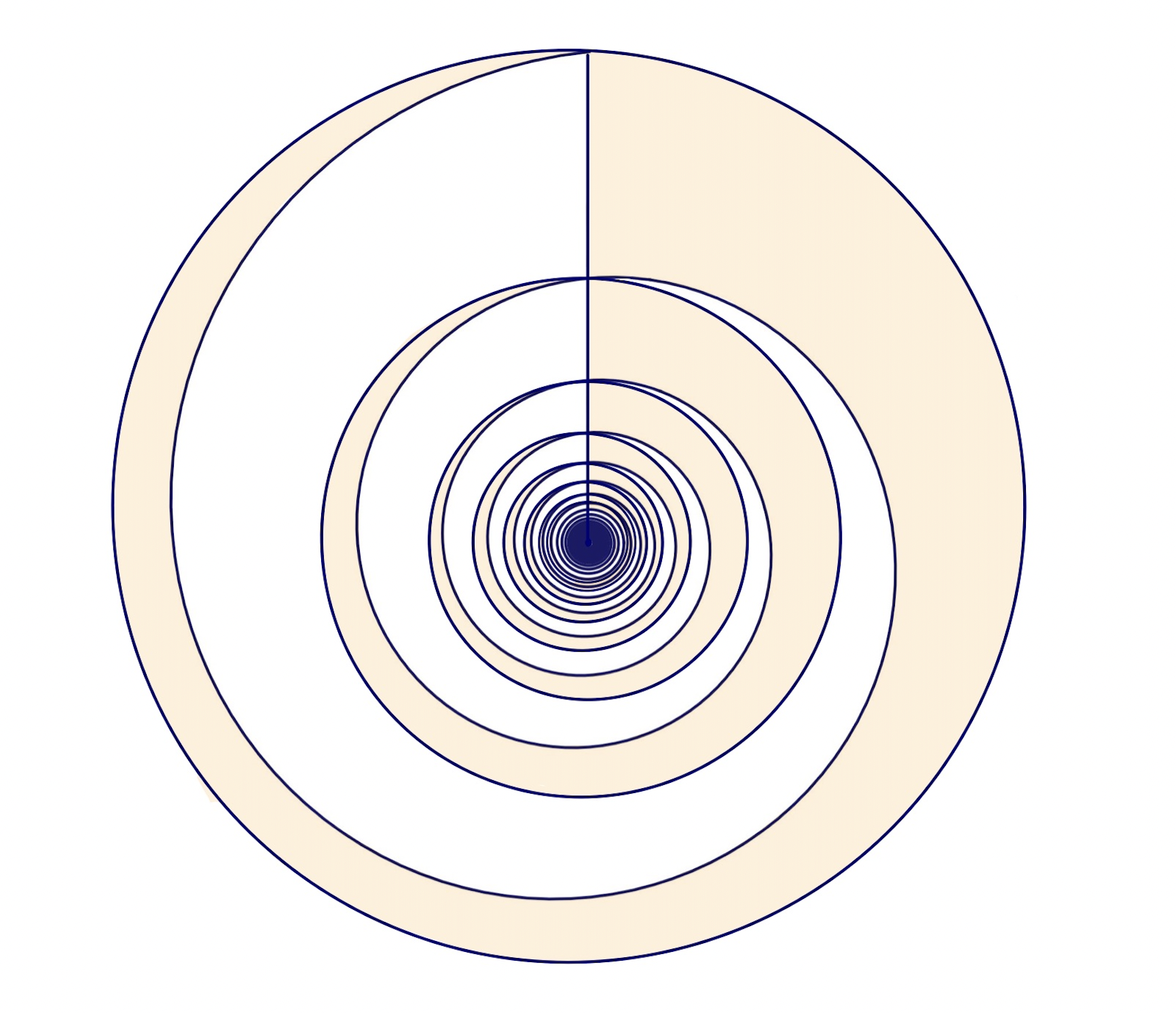
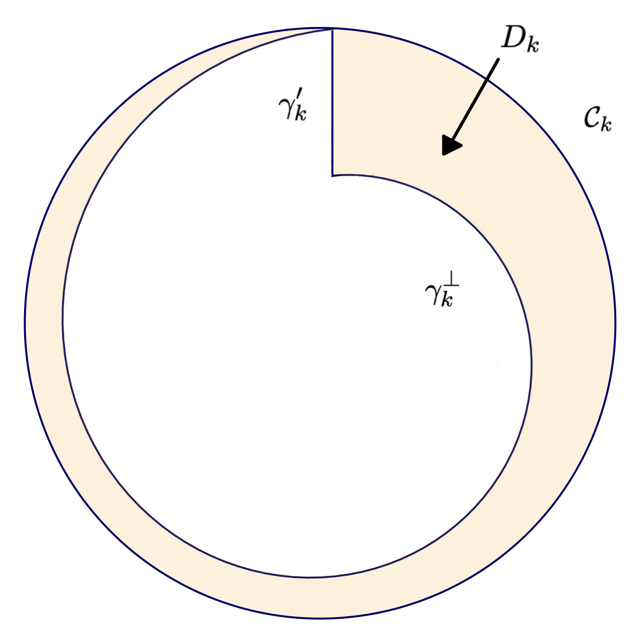
Figure 4: Left: The sequence of seashell domains (shaded), each component is enclosed between a circle, one revolution of the spiral, and a vertical line segment.
Right: A single seashell domain $D_{k}$, with the arcs $\gamma_{k}^{\prime}$, $\gamma_{k}^{\perp}$ and $\mathcal{C}_{k}$ indicated.

We continue our construction of a rectifiable Jordan arc $\Gamma_{\varepsilon}$ with superlinear growth of ${\sf Var}[\mathcal{E}_{\Lambda}(\Gamma)]$ when $\Lambda$ is the infinite Ginibre ensemble. For a given $\varepsilon>0$, we have found a curve $\mathcal{C}=\mathcal{C}_{\varepsilon}$ of the form

$$\mathcal{C}={\rm i}[0,\ell_{1}]\cup\bigcup_{k\geq 1}{\mathbb{D}}(0,\ell_{k})$$

such that

$${\sf Var}\left[\int_{R\mathcal{C}}V_{\Lambda}(z)\,{{\rm d}z}\right]\gtrsim R^{2-\varepsilon}.$$ (6.3)

We want to turn $\mathcal{C}$ into a Jordan arc with the bound (6.3) preserved. We do so by forming a spiral $\Gamma=\cup_{k\geq 1}\gamma_{k}$, where each revolution $\gamma_{k}$ interpolates between the intersection of successive circles $\mathcal{C}_{k}$ and $\mathcal{C}_{k+1}$ with the imaginary axis; i.e.

$$\gamma_{k}=\left\{\left(\ell_{k}(1-t)+\ell_{k+1}t\right)e^{2\pi{\rm i}t}:0\leq t\leq 1\right\}.$$

With the help of (6.3), we prove that

$${\sf Var}\left[\frac{1}{2\pi{\rm i}}\int_{R\Gamma}V_{\Lambda}(z)\,{{\rm d}z}\right]\gtrsim R^{2-\varepsilon}$$

as well. To see why this is so, we first recall that for the Ginibre point process, the (radial) two-point function $k_{\Lambda}(t)$ is given by

$$k_{\Lambda}(t)=-\pi^{-2}e^{-\pi t^{2}}\,,$$

see §2.4, Part I. Integration by parts yields

$$K(z)=4\int_{|z|}^{\infty}\log\Big{(}\frac{r}{|z|}\Big{)}re^{-\pi r^{2}}\,{{\rm d}}r=\frac{2}{\pi}\int_{|z|}^{\infty}e^{-\pi r^{2}}\,\frac{{\rm d}r}{r}\,,$$

which implies that

$$\bar{\partial}K(z)=\frac{e^{-\pi|z|^{2}}}{\pi\bar{z}}\in L^{1}({\mathbb{C}},{\rm d}m)\,.$$

We let $\gamma^{\prime}_{k}$ denote the short vertical segment $\gamma^{\prime}_{k}\stackrel{{\scriptstyle{\rm def}}}{{=}}\{{\rm i}t:\ell_{k+1}\leq t\leq\ell_{k}\}$. Then we obtain a closed curve by taking the union $\mathcal{C}_{k}\cup\gamma_{k}^{\perp}\cup\gamma^{\prime}_{k}$ (traversing $\mathcal{C}_{k}$ with its original orientation, and where $\gamma_{k}^{\perp}$ is $\gamma_{k}$ traversed backwards), which encloses a domain $D_{k}$; cf. Figure 4. All the domains $D_{k}$ are disjoint, and we denote their union by $D$ (the “seashell”).

By Green’s formula, we have for each $k\geq 0$ that

$$\int_{R(\mathcal{C}_{k}\cup\gamma_{k}^{\perp}\cup\gamma^{\prime}_{k})}K(|x-y|)\,{\rm d}y=2{\rm i}\int_{RD_{k}}\bar{\partial}_{y}K(|x-y|)\,{\rm d}m(y),$$

so that

$$\int_{R\gamma_{k}}K(|x-y|)\,{\rm d}y =-\int_{R\gamma_{k}^{\perp}}K(|x-y|)\,{\rm d}y$$

$$=\int_{R(\mathcal{C}_{k}\cup\gamma_{k}^{\prime})}K(|x-y|)\,{\rm d}y-2{\rm i}\int_{RD_{k}}\bar{\partial}_{y}K(|x-y|)\,{\rm d}m(y).$$

Adding up the contributions for $k\geq 0$, we obtain

$$\int_{R\Gamma}K(|x-y|)\,{\rm d}y =\int_{R(\mathcal{C}\cup i[0,\ell_{1}])}K(|x-y|)\,{\rm d}y-2{\rm i}\int_{RD}\bar{\partial}_{y}K(|x-y|)\,{\rm d}m(y)$$ (6.4)

$$=\int_{R\mathcal{C}}K(|x-y|)\,{\rm d}y+O(1),$$ (6.5)

where we have used that fact that $\bar{\partial}K\in L^{1}({\mathbb{C}},{\rm d}m)$. Integrating over $R\Gamma$, we find that

$$\iint_{R\Gamma\times R\Gamma}K(|x-y|)\,{\rm d}y{\rm d}\bar{x} =\int_{R\mathcal{C}}\left[\int_{R\Gamma}K(|x-y|)\,{\rm d}\bar{x}\right]{\rm d}y+O(R)$$ (6.6)

$$=\iint_{R\Gamma\times R\mathcal{C}}K(|x-y|)\,{\rm d}y{\rm d}\bar{x}+O(R).$$ (6.7)

Repeating the above argument, we finally arrive at

$$\iint_{R\Gamma\times R\Gamma}K(|x-y|)\,{\rm d}y{\rm d}\bar{x}=\iint_{R\mathcal{C}\times R\mathcal{C}}K(|x-y|)\,{\rm d}y{\rm d}\bar{x}+O(R),$$

from which the claim follows.

Acknowledgments

We are grateful to Fedor Nazarov, Alon Nishry and Ron Peled for several useful discussions throughout our work. We thank the anonymous referees for helpful comments.

Part of the work on this project was carried out while A.W. was based at Tel Aviv University. He would like to express his gratitude for the excellent scientific environment provided there.

The work of A.W. was supported by the KAW foundation grant 2017.0398, by ERC Advanced Grant 692616 and by Grant No. 2022-03611 from the Swedish Research Council (VR). The work of M.S. and O.Y. was supported by ERC Advanced Grant 692616, ISF Grant 1288/21 and by BSF Grant 202019.

Data availability statement

Data sharing not applicable to this article as no datasets were generated or analysed during the current study.

Compliance with ethical standards

The authors do not have any potential conflicts of interests to disclose.

Sodin: School of Mathematical Sciences, Tel Aviv University, Tel Aviv, Israel
sodin@tauex.tau.ac.il
Wennman: Department of Mathematics, KTH Royal Institute of Technology, Stockholm, Sweden
aronw@kth.se
Yakir: School of Mathematical Sciences, Tel Aviv University, Tel Aviv, Israel
oren.yakir@gmail.com

References

- [1] K. Adhikari, S. Ghosh, and J. L. Lebowitz, Fluctuation and entropy in spectrally constrained random fields, Comm. Math. Phys. 386 (2021), 749–780.
- [2] M. Björklund, T. Hartnick, Hyperuniformity and non-hyperuniformity of quasicrystals, Preprint, arXiv:2210.02151 (2022).
- [3] J. Buckley and M. Sodin, Fluctuations of the increment of the argument for the Gaussian Entire Function, J. Stat. Phys. 168 (2017), 300–330.
- [4] J. Dávila, On an open question about functions of bounded variation, Calc. Var. Partial Differential Equations 15 (2002), 519–527.
- [5] L. C. Evans and R. F. Gariepy, Measure theory and fine properties of functions. Revised, Textbooks in Mathematics, CRC Press, Boca Raton, FL, 2015.
- [6] S. Ghosh and J. L. Lebowitz, Fluctuations, large deviations and rigidity in hyperuniform systems: a brief survey, Indian J. Pure Appl. Math. 48 (2017), 609–631.
- [7] J. B. Hough, M. Krishnapur, Y. Peres and B. Virág, Zeros of Gaussian analytic functions and determinantal point processes. American Mathematical Society, Providence, RI, 2009.
- [8] B. Jancovici, Exact results for the two-dimensional one-component plasma, Phys. Rev. Lett. 46 (1981), 386–388.
- [9] B. Jancovici, J. L. Lebowitz, and G. Manificat, Large charge fluctuations in classical Coulomb systems, J. Stat. Phys. 72 (1993), 773–787.
- [10] J. Kim and S. Torquato, Effect of window shape on the detection of hyperuniformity via the local number variance, J. Stat. Mech. Theory Exp. (2017), p. 013402, 38.
- [11] J. L. Lebowitz, Charge fluctuations in Coulomb systems, Phys. Rev. E 27 (1983), 1491–1494.
- [12] Z. Lin, Nonlocal energy functionals and determinantal point processes on non-smooth domains, Preprint, arXiv:2304.00118 (2023).
- [13] V. A. Malyšev, A central limit theorem for Gibbsian random fields, Dokl. Akad. Nauk SSSR 224 (1975), 35–38.
- [14] P. A. Martin, Sum rules in charged fluids, Rev. Modern Phys. 60 (1988), 1075–1127.
- [15] P. A. Martin and T. Yalcin, The charge fluctuations in classical Coulomb systems, J. Statist. Phys. 22 (1980), 435–463.
- [16] P. Mattila, Geometry of sets and measures in Euclidean spaces. Cambridge University Press, 1995.
- [17] H. L. Montgomery, Ten lectures on the interface between analytic number theory and harmonic analysis. American Mathematical Society, Providence, RI, 1994.
- [18] F. Nazarov and M. Sodin, Correlation functions for random complex zeroes: strong clustering and local universality, Comm. Math. Phys. 310 (2012), 75–98.
- [19] M. Notarnicola, G. Peccati, A. Vidotto, Functional convergence of Berry’s nodal lengths: Approximate tightness and total disorder, Preprint, arXv:2208.07580 (2022).
- [20] C. Pommerenke, Boundary behaviour of conformal maps. Grundlehren der mathematischen Wissenschaften, 299. Springer-Verlag, Berlin, 1992.
- [21] M. Sodin, A. Wennman, and O. Yakir, The random Weierstrass zeta function I. Existence, uniqueness, fluctuations, Preprint, arXiv:2210.09882 (2022).
- [22] S. Torquato, Hyperuniform states of matter, Phys. Rep. 745 (2018), 1–95.
- [23] S. Torquato and F. H. Stillinger, Local density fluctuations, hyperuniformity, and order metrics, Phys. Rev. E (3) 68 (2003), pp. 041113, 25.
- [24] O. Yakir, Fluctuations of linear statistics for Gaussian perturbations of the lattice . J. Stat. Phys. 182 (2021), Paper No. 58, 21 pp.
Sodin:
School of Mathematical Sciences, Tel Aviv University, Tel Aviv, Israel