A Categorical Framework for Modeling with Stock and Flow Diagrams

Abstract

Stock and flow diagrams are already an important tool in epidemiology, but category theory lets us go further and treat these diagrams as mathematical entities in their own right. In this chapter we use communicable disease models created with our software, StockFlow.jl, to explain the benefits of the categorical approach. We first explain the category of stock-flow diagrams and note the clear separation between the syntax of these diagrams and their semantics, demonstrating three examples of semantics already implemented in the software: ODEs, causal loop diagrams, and system structure diagrams. We then turn to two methods for building large stock-flow diagrams from smaller ones in a modular fashion: composition and stratification. Finally, we introduce the open-source ModelCollab software for diagram-based collaborative modeling. The graphical user interface of this web-based software lets modelers take advantage of the ideas discussed here without any knowledge of their categorical foundations.

1 Introduction

Mathematical modeling of infectious disease at scale is important, but challenging. There are many benefits to the modeling process extending from taking diagrams as mathematical formalisms in their own right with the help of category theory. Stock and flow diagrams are widely used in infectious disease modeling, so we illustrate this point using these. However, rather than focusing on the underlying mathematics, we informally use communicable disease examples created with our software, called StockFlow.jl AlgebraicStockFlow , to explain the benefits of the categorical framework. Readers interested in the mathematical details may refer to our earlier paper baez2022compositional .

Many compartmental modelers regard diagrams offering a visual characterization of structure—e.g., susceptible, infective and recovered stocks and transitions between them—as broadly accessible but informal steps towards a mathematically rigorous formulation in terms of ordinary differential equations (ODEs). However, ODEs are typically opaque to non-modelers—including the interdisciplinary members of the teams that typically are required for impactful models. By contrast, the System Dynamics modeling tradition places a premium on engagement with stakeholders hovmandCBSD , and offers a modeling approach centered around diagrams. This approach commonly proceeds in a manner that depicts model structure using successively more detailed models. The process starts with a “causal loop diagram” illustrating causal connections and feedback loops (Figure 6). It then often proceeds to a “system structure diagram”, which distinguishes stocks from flows but still lacks quantitative information. The next step is to construct a stock and flow diagram—or henceforth, “stock-flow diagram” (Figure 1). This diagram is visually identical to the system structure diagram, but it also includes formulae, values for parameters, and initial values of stocks.

The stock–flow diagram is treated as the durable end result of this modeling process, since it uniquely specifies a system of first-order ODEs. System Dynamics modeling typically then alternates between assessing scenario outcomes resulting from numerically integrating the ODEs, performing other analyses (e.g., identifying location or stability of equilibria), and elaborating the stock-flow diagram—such as by adding elements to it, often borrowed from other models, or “stratifying” it by breaking large stocks (compartments) into smaller ones that differ in some characteristics.

While each of the types of diagrams in the System Dynamics tradition is recommended by visual accessibility, development of models using the traditional approach suffers from a number of practical shortcomings.

1. Monolithic models: Stock-flow models are traditionally built up in a monolithic fashion, leading ultimately to a single large piece of code. In larger models, this inhibits independent simultaneous work by multiple modelers. Lack of model modularity further prevents effective reuse of particular model elements. If elements of other models are used, they are commonly copy-and-pasted into the developing model, with the source and destination then evolving independently. Such separation can lead to a proliferation of conceptually overlapping models in which a single conceptual change (e.g., addition of a new asymptomatic infective compartment) requires corresponding updates in several successive models.

2. Curse of stratification dimensionality: While stratification is a key tool for representing heterogeneity and multiple lines of progression in compartmental models, stratification commonly requires modifications across the breadth of a model—stocks, flows, derived quantities, and many parameters. When that stratification involves multiple dimensions of heterogeneity, it can lead to a proliferation of terms in the ODEs. For example, rendering a model characterizing both COVID-19 into a model also characterizes influenza would require that each COVID-19 state to be replicated for each stage in the natural history of influenza. Represented visually, this stratification leads to a multi-dimensional lattice, commonly with progression proceeding along several dimensions of the lattice. Because of the unwieldy character of the diagram, much of the structure of the model is obscured. Adding, removing, or otherwise changing dimensions of heterogeneity routinely leads to pervasive changes across the model.

3. Privileging ODE semantics: The structure of causal loop diagrams, system structure diagrams and stock-flow diagrams characterizes general state and accumulations, transitions and posited causal relations—including induced feedbacks—amongst variables. Nothing about such a characterization restricts its meaning to ordinary differential equations; indeed, many other interpretations and uses of these diagrams are possible. However, existing software privileges an ODE interpretation for stock-flow diagrams, while sometimes allowing for secondary analyses in ad hoc way—for example, identifying causal loops associated with the model, or verifying dimensional homogeneity in dimensionally annotated models. Conducting other sorts of analyses—such as computation of eigenvalue elasticities or loop gains, analysis as a stochastic transition system, or other methods such as particle filtering Arulampalam2002-xj ; li2018applyingMeasles ; OsgoodLiuPF2014 ; safarishahrbijari2017predictive , particle MCMC andrieuDoucet2010PMCMC ; opioids_li2018illuminating ; SSC_OsgoodEng2022 or Kalman filtered gelb1974applied ; WinchellKalman systems—typically requires bespoke software for reading, representing and analyzing stock-flow models.

4. Divergence of model representations: Although the evolution from causal loop diagrams to system structure diagrams to stock-flow models is one of successive elaboration and informational enrichment, existing representations treat these as entirely separate characterizations and fail to capture the logical relationships between them. Such fragmentation commonly induces inconsistent evolution. Indeed, in many projects, the evolution of stock-flow diagrams renders the earlier, more abstract formulations obsolete, and the focus henceforth rests on the stock-flow diagrams.

What is less widely appreciated is that beyond their visual transparency and capacity to be lent a clear ODE semantics, both stock-flow diagrams themselves and their more abstract cousins possess a precise mathematical structure—a corresponding grammar, as it were. This algebraic structure, called the “syntax” of stock-flow diagrams, can be characterized using the tools of a branch of mathematics called category theory SevenSketches ; leinster . Formalizing the syntax of stock-flow diagrams lends precise meaning to the process of “composing” such models (building them out of smaller parts), stratifying them, and other operations. Explicitly characterizing the syntax in software also allows for diagrams to be represented, manipulated, composed, transformed, and flexibly analyzed in software that implements the underlying mathematics.

Formalizing the mathematics of diagram-based models using category theory and capturing it in software offers manifold benefits. This paper discusses and demonstrates just a few:

1. Separation of syntax and semantics. Category theory gives tools to separate the formal structure, or “syntax”, of diagram-based models from the uses to which they are put, or “semantics”. This separation permits great flexibility in applying different semantics to the same model. With appropriate software design, this decoupling can allow the same software to support a diverse array of analyses, which can be supplemented over time.

2. Reuse of structure. The approaches explored here provide a structured way to build complex diagrams by composing small reusable pieces. With software support, modeling frameworks can allow for saving models and retrieving them for reuse as parts of many different models. For example, a diagram representing contact tracing processes can be reused across diagrams addressing different pathogens.

3. Modular stratification. A categorical foundation further supports a structured way to build stratified dynamical systems out of modular, reusable, largely orthogonal pieces. In contrast to the global changes commonly required to a diagram and the curse of dimensionality that traditionally arises when stratifying a diagram, categorically-founded stratification methods allow for crisply characterizing a stratified diagram as built from simpler diagrams, one for each heterogeneity or progression dimension.

The balance of the chapter is structured as follows. Section 2 describes the categorical formulation of stock-flow diagrams. Section 3 explains how the categorical approach allows for decoupling the syntax and semantics of such diagrams. Section 4 introduces the hallmark of the categorical approach: the ability to build larger stock-flow diagrams from smaller pieces by composition. Section 5 discusses another key application of the categorical approach: stratification. Section 6 introduces ModelCollab: a web-based graphical user interface that allows users to build and run stock-flow models using the category-theoretic ideas we have introduced without requiring expertise in the mathematics. Finally, in Section 7 we close with some reflections on the significance and evolution of the methods described here. The code for examples in this paper can be found in the Appendix.

2 The Syntax of Stock-Flow Diagrams

In this section, we illustrate the categorical method of representing stock-flow diagrams, which we can think of as characterizing the syntax of such diagrams. Section 3 of our previous work baez2022compositional introduced the mathematics underlying stock-flow diagrams. In this paper, we show how to encode an instance of a familiar stock-flow diagram—namely, the Susceptible-Exposure-Infectious-Recovered or “SEIR” model with an open population anderson1992infectious —using the categorical method.

Figure 1: The stock-flow diagram of the open population SEIR model

Figure 1 shows the stock-flow diagram for the SEIR model. The blue boxes labeled S, E, I and R are “stocks”. The letter N is a “sum variable”, and there are blue “links” to it from the stocks on which it depends. The orange arrows are “flows”. Note that some flows go between stocks, while others enter a stock from outside the model, or leave a stock to go outside the model. The latter two cases are indicated with small “clouds”.

There are one or more blue links to each flow from the stocks and/or sum variables on which it depends. For each flow there is also a “flow variable” drawn in purple, which indicates the rate of that flow. Each flow variable is determined by some function of the stocks and/or sum variables that are connected to that flow variable by blue links. These functions are defined below the diagram in Figure 1. For example, the flow describing infection, called inf, has a flow variable vinf determined by the function $f_{\textrm{inf}}$.

[width=0.5]fig/schema_stockflow.jpg

Figure 2: The schema for stock-flow diagrams

The SEIR model is just one example of a stock-flow diagram. To formalize their general structure we use the so-called “schema” for stock-flow diagrams, shown in Figure 2. It consists of boxes, called “objects”, and arrows between boxes, called “morphisms”. In an “instance” of this schema, we choose a set for each object and a function between such sets for each morphism. Other types of diagrams, such as causal loop diagrams, have their own schemas (see Section 3.2), and in fact there is a general theory of schemas SevenSketches ; spivak2014category . For now we consider only the schema for stock-flow diagrams. In this schema:

1. The objects $\mathrm{S}$ and $\mathrm{F}$ represent the stocks and flows, respectively.

2. The objects $\mathrm{I}$ and $\mathrm{O}$ represent the inflows and outflows. The morphisms $\mathrm{S}\xleftarrow{\mathrm{is}}\mathrm{I}\xrightarrow{\mathrm{ifn}}\mathrm{F}$ are used to describe which stocks are downstream of a given flow, while the morphisms $\mathrm{S}\xleftarrow{\mathrm{os}}\mathrm{O}\xrightarrow{\mathrm{ofn}}\mathrm{F}$ are used to describe which stocks are upstream of a given flow. This structure allow for flows that go between two stocks, but also flows that enter a stock from outside the model or leave a stock and go outside the model.

3. The object $\mathrm{V}$ represents “auxiliary variables”, sometimes termed “dynamic variables”. These are variables whose value is an instantaneous function of the current model state. The morphism $\mathrm{F}\xrightarrow{\mathrm{fv}}\mathrm{V}$ indicates that the rate of each flow depends on one auxiliary variable. This relation is usually left implicit, not drawn, in the stock-flow diagram.

4. The object $\mathrm{LV}$ represents “variable links”: that is, links from stocks to auxiliary variables. The morphisms $\mathrm{S}\xleftarrow{\mathrm{lvs}}\mathrm{LV}\xrightarrow{\mathrm{lvv}}\mathrm{V}$ indicate that any variable link goes from a stock to an auxiliary variable.

5. The objects $\mathrm{SV}$ and $\mathrm{LS}$ represent “sum variables” and “sum links”. Sum variables are a special type of auxiliary variable introduced in baez2022compositional to make composing stock-flow diagrams easier. A sum variable is simply the sum of the stocks linked to them by sum links. The arrows $\mathrm{S}\xleftarrow{\mathrm{lss}}\mathrm{LS}\xrightarrow{\mathrm{lssv}}\mathrm{SV}$ indicate that any sum link goes from a stock to a sum variable.

6. The object $\mathrm{LSV}$ represents “sum variable links”: that is, links from sum variables to auxiliary variables. The arrows $\mathrm{SV}\xleftarrow{\mathrm{lsvsv}}\mathrm{LSV}\xrightarrow{\mathrm{lsvv}}\mathrm{V}$ indicate that any sum variable link goes from a sum variable to an auxiliary variable.

An “instance” $G$ of a schema assigns a finite set $G(\mathsf{X})$ to each object $\mathsf{X}$ of the schema and a function $G(a)\colon G(\mathsf{X})\to G(\mathsf{Y})$ to each morphism $\mathsf{X}\xrightarrow{a}\mathsf{Y}$ of the schema. So, an instance of the schema for stock-flow diagrams consists of:

1. A finite set of stocks $G(\mathrm{S})$ and a finite set of flows $G(\mathrm{F})$.

2. A finite set of inflows $G(\mathrm{I})$, a finite set of outflows $G(\mathrm{O})$, and functions

   $$G(\mathrm{is})\colon G(\mathrm{I})\to G(\mathrm{S}),\qquad G(\mathrm{ifn})\colon G(\mathrm{I})\to G(\mathrm{F})$$

   $$G(\mathrm{os})\colon G(\mathrm{O})\to G(\mathrm{S}),\qquad G(\mathrm{ofn})\colon G(\mathrm{O})\to G(\mathrm{F}).$$

3. A finite set of auxiliary variables $G(\mathrm{V})$ and a function

   $$G(\mathrm{fv})\colon G(\mathrm{F})\to G(\mathrm{V}).$$

4. A finite set of variable links $G(\mathrm{LV})$ and functions

   $$G(\mathrm{lvs})\colon G(\mathrm{LV})\to G(\mathrm{S}),\qquad G(\mathrm{lvv})\colon G(\mathrm{LV})\to G(\mathrm{V}).$$

5. A finite set of sum variables $G(\mathrm{SV})$, a finite set of sum links $G(\mathrm{LS})$, and functions

   $$G(\mathrm{lss})\colon G(\mathrm{LS})\to G(\mathrm{S}),\qquad G(\mathrm{lssv})\colon G(\mathrm{LS})\to G(\mathrm{SV}).$$

6. A finite set of sum variable links $G(\mathrm{LSV})$ and functions

   $$G(\mathrm{lsvsv})\colon G(\mathrm{LSV})\to G(\mathrm{SV}),\qquad G(\mathrm{lsvv})\colon G(\mathrm{LSV})\to G(\mathrm{V}).$$

A “stock-flow diagram” is a pair $(G,\phi)$ consisting of an instance $G$ and, for each auxiliary variable $v$, a continuous function $\phi_{v}\colon\mathbb{R}^{G(\mathrm{lvv})^{-1}(v)}\times\mathbb{R}^{G(\mathrm{lsvv})^{-1}(v)}\to\mathbb{R}$. In Section 3.1 we explain how in the ODE semantics for stock-flow diagrams, the function $\phi_{v}$ specifies how the value of the variable $v$ depends on the stocks and sum variables that link to it.

Given an inflow $i\in G(\mathrm{I})$ we say the stock $G(\mathrm{is})(i)$ is “downstream” from the flow $G(\mathrm{ifn})(i)$. Similarly, given an outflow $o\in G(\mathrm{O})$ we say the stock $G(\mathrm{os})(o)$ is “upstream” from the flow $G(\mathrm{ofn})(o)$. In practice, we only want stock-flow diagrams where the functions $G(\mathrm{ifn})$ and $G(\mathrm{ofn})$ are injective. This constraint ensures that each flow has at most one downstream stock and at most one upstream stock. Also in practice we attach to each stock, flow, auxiliary variable or sum variable an “attribute” which serves as its name. This naming relies on the theory of attributes developed by Patterson, Lynch and Fairbanks patterson-lynch-fairbanks2021 .

Figure 3: The categorical database structure representing the stock-flow diagram associated with the SEIR model

When a stock-flow diagram is implemented in software, it is encoded as a categorical database patterson-lynch-fairbanks2021 . Figure 3 shows the categorical database representing the stock-flow diagram for the SEIR model shown in Figure 1. In this categorical database, each object $\mathsf{X}$ in the schema for stock-flow diagrams is represented by a database table. The row indices within this table consist of the elements of the set $G(\mathsf{X})$ associated to the object $\mathsf{X}$. Thus, if the set $G(\mathsf{X})$ has $n$ elements, then the table has $n$ rows. In database parlance, each such row is associated with a “primary key” given in the first column of that table. For example, since there are four stocks in the SEIR model, the object $\mathrm{S}$ in the schema for stock-flow diagrams maps to the set $\{1,2,3,4\}$, and the table for the object $\mathrm{S}$ has four rows numbered $1,2,3,4$. By contrast, the table for the object $\mathrm{F}$ has eight rows, reflecting the fact that there are eight flows in the SEIR model.

The table for any object $\mathsf{X}$ has one column for each morphism coming out of $\mathsf{X}$, which describes the function associated to that morphism. For example, the table for the object $\mathrm{LV}$ has one column “$\mathrm{lvs}$” describing the function $G(\mathrm{lvs})\colon G(\mathrm{LV})\to G(\mathrm{S})$ mapping each variable link to a stock (as a “foreign key” giving the key of that stock in the “S” table), and one column “$\mathrm{lvv}$” describing the function $G(\mathrm{lvv})\colon G(\mathrm{LV})\to G(\mathrm{V})$ mapping each variable link to a variable (similarly specified by a foreign key). Besides this, the tables for $\mathrm{S},\mathrm{F},\mathrm{V}$ and $\mathrm{SV}$ have an extra column giving names for the stocks, flows and variables and sum variables, rather than foreign keys. Technically, these names are handled using the theory of attributes mentioned above.

This capacity to encode stock-flow diagrams in a mathematically precise and transparent fashion confers diverse benefits. To list a few, these include the capacity to compose such diagrams (see Section 4), to soundly transform such diagrams for optimization, and to parallelize them. But one of the most foundational benefits is the capacity to perform different types of analysis on such diagrams—that is, to interpret a given diagram using various choices of “semantics”. The next section discusses that benefit in greater detail.

3 The Semantics of Stock-Flow Diagrams

The capacity to interpret stock-flow diagrams in different ways is achieved by separating the syntax from the semantics of such diagrams. Matters of syntax concern the forms that such diagrams can take. In particular, the rules governing what counts as a legitimate stock-flow diagram—what can connect to what—are largely specified by the schema discussed in the previous section. But the syntax of stock-flow diagrams is distinct from the interpretation given to these diagrams. A given stock-flow diagram can be interpreted in different ways, each lending that diagram some meaning. Some of these interpretations involve dynamic simulations that solve equations specified by the diagram, whilst others describe static features of the diagram—for example, extracting algebraic equations specifying the equilibria of the system in terms of the parameters.

In this section, we introduce three choices of semantics for stock-flow diagrams that have been implemented in StockFlow.jl baez2022compositional ; AlgebraicStockFlow : ordinary differential equations, and a pair of semantics that extract from a stock-flow diagram the associated causal loop diagram and system structure diagram.

3.1 ODEs (Ordinary Differential Equations)

A stock-flow diagram is traditionally used to represent a continuous-time, continuous-state dynamical system sterman2000business : a system of ODEs that describes the evolution of each real-valued stock. While this addresses an important subclass of dynamical systems, this convention has needlessly restricted analysis potential and crimped the flexibility of supporting software by privileging a single interpretation of the syntax of the stock-flow diagrams. In this project, we mathematically decouple the choice of the stock-flow diagram (the syntax) from the choice of its interpretation (the semantics). As we shall see in this subsection, this approach readily supports the traditional interpretation of a stock-flow diagram in terms of ODEs. But as subsequent subsections illustrate, this interpretation is no longer required, or even privileged.

The decoupling of syntax and semantics afforded by the categorical approach is achieved by use of a structure-preserving map, called a “functor”, sending each stock-flow diagram to its interpretation, or meaning. The choice of different such functors allows for different interpretations.

“Functorial semantics”—the idea of treating semantics as a functor—goes back to Lawvere’s work lawvere1963functorial in the early 1960s. It has grown into a powerful method for specifying and analyzing the semantics of programming languages. By now, it has also been applied to many diagrammatic modeling languages, including Petri nets, electrical circuit diagrams and chemical reaction networks, and others baezcourser2020 ; baez-courser-vasilakopoulou2022 ; fongthesis . Thus, the time is ripe for applying functorial semantics to stock–flow diagrams.

To do this, we need to define a category of stock-flow diagrams, which in essence means precisely defining not only these diagrams, as we have done above, but also maps between them. Using the methods of our previous paper baez2022compositional we can define such a category, called $\mathsf{StockFlow}$, and also a functor

from this category to a category of ODEs and maps between those. Here, for simplicity, we simply explain how this functor sends any stock-flow diagram to an ODE.

For any stock $s\in G(\mathrm{S})$, the set of its inflows is $G(\mathrm{is})^{-1}(s)$. Thus, this stock is downstream from precisely the flows in $G(\mathrm{ifn})(G(\mathrm{is})^{-1}(s))$. Similarly, this stock is upstream from precisely the flows in $G(\mathrm{ofn})(G(\mathrm{os})^{-1}(s))$. We denote as $\phi_{v}$ the continuous function describing the value of each auxiliary variable $v\in G(\mathrm{V})$ as a function of the stocks and sum variables linked to it, so $\phi_{v}\colon\mathbb{R}^{G(\mathrm{lvv})^{-1}(v)}\times\mathbb{R}^{G(\mathrm{lsvv})^{-1}(v)}\to\mathbb{R}$. Then, the function describing the rate of the flow $f\in G(\mathrm{F})$ is $\phi_{(G(\mathrm{fv})(f))}$. The ordinary differential equation of the stock $s$ can then be defined as follows:

$$\dot{s}=\sum_{f\in G(\mathrm{ifn})(G(\mathrm{is})^{-1}(s))}\phi_{(G(\mathrm{fv})(f))}-\sum_{f\in G(\mathrm{ofn})(G(\mathrm{os})^{-1}(s))}\phi_{(G(\mathrm{fv})(f))},$$ (1)

Furthermore the value of each sum auxiliary variable is the sum of the values of the stocks it links to. For example, the value of the sum variable $N$ is defined as $N=S+E+I+R$ in the SEIR model.

We can easily understand the functor mapping from a stock-flow diagram to the ODEs by the slogan: the time derivative of the value of each stock equals the sum of its inflows minus the sum of its outflows.

For example, the SEIR stock-flow diagram (Figure 1) gives the following set of ODEs:

$$\begin{split}\dot{S}&=\mu N-\beta\frac{I}{N}S-\delta S\\ \dot{E}&=\beta\frac{I}{N}S-\frac{E}{t_{\text{latent}}}-\delta E\\ \dot{I}&=\frac{E}{t_{\text{latent}}}-\frac{I}{t_{\text{recovery}}}-\delta I\\ \dot{R}&=\frac{I}{t_{\text{recovery}}}-\delta R\end{split}$$ (2)

The solutions can be calculated and plotted out directly using the StockFlow.jl software, as in Figure 4.

[width=0.6]fig/ODEsSolution.jpg

Figure 4: An example solution of the ODEs of the SEIR stock-flow diagram

It is notable that the ODE semantics mapping is more general than illustrated above: we can also map the syntax of “open” stock-flow diagrams (to be discussed in Section 4) to “open” dynamical systems. This supports composition of models.

3.2 Causal Loop Diagrams

In this section, we define a semantics for stock-flow diagrams that maps any such diagram into a particularly simple kind of causal loop diagram. In System Dynamics, a “causal loop diagram” is a graph where each node represents a variable and each edge represents a way in which one variable can directly influence another sterman2000business . The edges are typically labelled with $\pm$ signs called “polarities” that indicate whether an increase in the source variable tends to increase or decrease the target variable, ceteris paribus. From these we can compute signs for loops of edges, which describe positive or negative feedback loops.

Here we consider a simplified variant of causal loop diagram which is simply a graph: the polarities for edges are not included. The problem of interpreting a stock-flow diagram as a fully annotated causal loop diagram is left for future work.

[width=0.4]fig/schema_causalLoop.jpg

Figure 5: The schema for causal loop diagrams

Figure 5 depicts the schema for causal loop diagrams. It is just the schema for what category theorists call “graphs” (that is, directed multigraphs allowing self-loops). There is an object $\mathrm{E}$ for edges, an object $\mathrm{N}$ for nodes, and morphisms $s,t\colon\mathrm{E}\to\mathrm{N}$ sending each edge to its source and target node, respectively. Thus, an instance $\mathrm{CL}$ of this schema is simply a finite set $\mathrm{CL}(\mathrm{N})$ of nodes, a finite set $\mathrm{CL}(\mathrm{E})$ of edges, and maps $\mathrm{CL}(s),\mathrm{CL}(t)\colon\mathrm{CL}(\mathrm{E})\to\mathrm{CL}(\mathrm{N})$ sending each edge to its source and target node.

There is in fact a way to translate any stock-flow diagram $(G,\phi)$ into a causal loop diagram $\mathrm{CL}$. It works as follows:

1. The set of nodes $\mathrm{CL}(\mathrm{N})$ is the disjoint union of the set of stocks, the set of sum variables, and the set of auxiliary variables (which includes such a variable for each flow). Explicitly,

   $$\mathrm{CL}(\mathrm{N})\coloneqq\mathsf{G}(\mathrm{S})\sqcup\mathsf{G}(\mathrm{SV})\sqcup\mathsf{G}(\mathrm{V}).$$

2. The set of edges $\mathrm{CL}(\mathrm{E})$ is given by

   $$\mathrm{CL}(\mathrm{E}):=\mathsf{G}(\mathrm{LV})\sqcup\mathsf{G}(\mathrm{LS})\sqcup\mathsf{G}(\mathrm{LSV})\sqcup\mathsf{G}(\mathrm{I})\sqcup\mathsf{G}(\mathrm{O}).$$

3. Each edge coming from a variable link $\ell\in\mathsf{G}(\mathrm{LV})$ has source $\mathsf{G}(\mathrm{lvs})(\ell)$ and target $\mathsf{G}(\mathrm{lvv})(\ell)$. The source and target of edges coming from sum links and sum variable links are defined similarly. Each edge coming from an inflow $i\in\mathsf{G}(\mathrm{I})$ has the auxiliary variable $\mathsf{G}(\mathrm{fv})\mathsf{G}(\mathrm{ifn})(i)$ as its source and the stock $G(\mathrm{is})(i)$ as its target. Note that the auxiliary variable $\mathsf{G}(\mathrm{fv})\mathsf{G}(\mathrm{ifn})(i)$ represents the flow for which $i$ is the inflow. Similarly, each edge coming from an outflow $o\in\mathsf{G}(\mathrm{O})$ has the stock $G(\mathrm{os})(o)$ as its source and the auxiliary variable $\mathsf{G}(\mathrm{fv})\mathsf{G}(\mathrm{ofn})(o)$ as its target.

Using this procedure, the SEIR stock-flow diagram in Figure 1 gives rise to the causal loop diagram in Figure 6. Here, following tradition, we have labeled some of the nodes by flows rather than their corresponding auxiliary variables, e.g. “birth” rather than “vbirth”. Since the map $\mathsf{G}(\mathrm{fv})\colon\mathsf{G}(\mathrm{F})\to\mathsf{G}(\mathrm{V})$ is usually one-to-one, this does not create ambiguities in practice.

[width=0.6]fig/causalLoop_SEIR.jpg

Figure 6: The causal loop diagram of the SEIR model

Just as with stock-flow diagrams, we use the data structure of a categorical database to encode causal loop diagrams in the software. Figure 7 shows an example: the categorical database for the SEIR causal loop diagram.

[width=0.6]fig/schema_database_causalloop_SEIR.jpg

Figure 7: The categorical database structure representing the SEIR causal loop diagram

3.3 System Structure Diagrams

In System Dynamics sterman2000business , a system structure diagram is a purely qualitative version of a stock-flow diagram. It lacks the quantitative information provided by the functions $\phi_{v}$ that describe how each auxiliary variable $v$ depends on the quantities linked to it. While many uses of system structure diagrams further annotate links in such diagrams with polarities, we reserve for future work the problem of automatic derivation of such polarities. For now, we therefore define a “system structure diagram” to be simply an instance $G$ of the schema for stock-flow diagrams, as explained in Section 2.

There is a semantics for stock-flow diagrams that maps them to system structure diagrams: it simply maps any stock-flow diagram $(G,\phi)$ to the system structure diagram $G$. In fact one can construct a category $\mathsf{StockFlow}$ of stock-flow diagrams, a category $\mathsf{SystemStructure}$ of system structure diagrams, and a functor

that maps any stock-flow diagram $(G,\phi)$ to the system structure diagram $G$.

Likewise, the semantics described in Section 3.2 gives a functor

from the category of stock-flow diagrams to a suitable category $\mathsf{CausalLoop}$. But note that the causal loop diagram associated to a stock-flow diagram $(G,\phi)$ depends only on $G$: the functions $\phi_{v}$ play no role here, though they would for the more elaborate and more commonly used causal loop diagrams with edges labeled by polarities. Thus, our causal loop and system structure semantics for stock-flow diagrams fit into a so-called “commutative diagram” of functors between categories:

In essence, this diagram says that to turn a stock-flow diagram $(G,\phi)$ into a causal loop diagram in the manner explained in Section 3.2, we can first extract the system structure diagram $G$ and then turn that into a causal loop diagram.

This commutative diagram illustrates a general fact: rather than the various semantics for a given form of syntax being separate from each other, like isolated walled gardens, they are often related in fruitful ways. Category theory lets us formalize these relationships, and category-based software lets us apply them in practical ways.

4 Composing Open Stock-Flow Diagrams

We can build larger stock-flow diagrams by gluing together smaller ones. To achieve this goal, we need “open” stock-flow diagrams. An example is shown in Figure 8. It consists of a stock-flow diagram together with some extra data describing interfaces at which we can compose this diagram to other stock-flow diagrams.

Figure 8: An example of an open stock-flow diagram

More precisely, an open stock-flow diagram consists of an “apex” together with a finite collection of “feet” and “legs”. The “apex” is any stock-flow diagram $(G,\phi)$. Each “foot” is also a stock-flow diagram, and it comes with a “leg”, which is a map of stock-flow diagrams from the foot to $(G,\phi)$. However, we require that the feet are stock-flow diagrams of a restricted sort: they can contain only stocks, sum variables and sum links. We enforce this restriction because we want to glue together stock-flow diagrams only by identifying certain stocks in one diagram with stocks in another diagram; however, doing this properly may require identifying certain sum variables and sum links as well.

[width=0.35]fig/foot_schema.jpg

Figure 9: The schema for interfaces

We call these restricted stock-flow diagrams “interfaces”. Just as there is a schema for stock-flow diagrams, there is a schema for interfaces, shown in Figure 9. An interface, say $X$, is precisely an instance of this schema. It thus consists of:

1. a finite set $X(\mathrm{S})$ of stocks,

2. a finite set of sum variables $X(\mathrm{SV})$, a finite set of sum links $X(\mathrm{LS})$, and functions

   $$X(\mathrm{lss})\colon X(\mathrm{LS})\to X(\mathrm{S}),\qquad X(\mathrm{lssv})\colon X(\mathrm{LS})\to X(\mathrm{SV}).$$

In our previous paper baez2022compositional we explain how to compose open stock-flow diagrams. Briefly, we use the mathematics of “decorated cospans” fong2015 —a general category-theoretic framework for the composition of open systems. However, to implement this in code in StockFlow.jl we also take advantage of a closely related framework, “structured cospans” baezcourser2020 ; baez-courser-vasilakopoulou2022 . The reason is that structured cospans have already been systematically implemented in the Catlab.jl package patterson-lynch-fairbanks2021 , which serves as the foundation underlying our implementation of StockFlow.jl. StockFlow.jl is one of the newer members of the AlgebraicJulia ecosystem AlgebraicJulia , which provides computational support for applied category theory via Catlab.jl.

Two other twists are also worth noting, if only for cognoscenti. Firstly, in StockFlow.jl we actually use decorated or structured “multicospans” libkind-baas-patterson-fairbanks2021 ; spivak2013 instead of cospans. The difference is that multicospans can have multiple legs and feet, as shown for example in Figure 8, while cospans have exactly two. Secondly, StockFlow.jl applies the flexible graphical syntax of undirected wiring diagrams fongspivak2018 to compose these multicospans.

However, users do not need to understand these technicalities to use our software. The key ideas can be understood from an example. Figure 8 shows an open stock-flow diagram with three legs and feet: this is an SEIR model with three interfaces containing the stocks $\mathrm{S},\mathrm{E}$ and $\mathrm{I}$, respectively. Figure 10 shows an example of composition in which this open stock-flow diagram is glued to another open stock-flow diagram, an SVEI model, along all three interfaces. The result of composition is yet another open stock-flow diagram, but in this particular case there are no interfaces left, so it amounts to an ordinary stock-flow diagram. The composite diagram describes an SEIRV model. Like any other diagram, diagrams that result from such composition can be mapped to alternative semantic domains. For example, the bottom right plot in Figure 10 then shows a solution of the system of ODEs to which the composite stock-flow diagram is mapped using ODE semantics.

Figure 10: Composing SEIR and SVEI models to obtain an SEIRV model

5 Stratifying Typed System Structure Diagrams

Just as we introduced open stock-flow diagrams to permit composition of models, we now introduce typed diagrams to support stratification of models. Recall from Section 1 that “stratifying” a model involves breaking stocks into smaller stocks that differ in some characteristics. For example, we might take the simple SEIR model shown in Figure 1 and subdivide each stock into two groups of different sexes, or three groups of different ages, or both. This subdivision is a common and important procedure for refining models in epidemiology.

However, stratification also requires introducing new flows, new auxiliary variables, new links, and so on. For example, consider the flow “inf” from the “Exposed” stock to the “Infectious” stock in the SEIR model. If we stratify this model by breaking each stock into two sexes, we also need to replace this flow with two separate flows, one for each sex. Furthermore, since the rate of this flow is given by an auxiliary variable, we must replace that variable by two separate variables if we wish to allow the two sexes to have different rates of infection—which indeed is the whole point of stratifying the model in this way.

The challenge is to carry out all these steps in a mathematically well-defined way that can be cleanly implemented in software. Libkind et al. recently did this for a related diagrammatic modeling language that has also been implemented in the AlgebraicJulia ecosystem: Petri nets libkind2022epidemic . The key was to introduce “typed” Petri nets and use pullbacks, a standard construction in category theory leinster . However, their approach to stratification has the potential to be generalized to many other diagrammatic modeling languages. Here we adapt their approach to stock-flow diagrams.

To begin, it is important to realize that when we stratify a model described by a stock-flow diagram $(G,\phi)$, we do not expect that all the functions $\phi_{v}$ associated to auxiliary variables $v$ can be copied over from the original model in an automatic way. Indeed, the point of stratification is to let these functions depend on the “stratum”, e.g. the sex, the age group, and so on. Thus, in the approach we take here, we first stratify not the whole stock-flow diagram $(G,\phi)$ but only its underlying system structure diagram $G$ (as defined in Section 3.3). To promote the stratified system structure diagram to a stock-flow diagram, the user must then choose functions for the auxiliary variables. In future work, we can enable an approach where most, but not all, of the original functions are automatically reused.

How do we stratify system structure diagrams? A first naive thought would be to take a “product” of two system structure diagrams:

1. The original system structure diagram that we wish to stratify. We call this the “aggregate model” and denote it as $S_{\textrm{aggregate}}$.

2. A system structure diagram describing the strata (e.g., age groups or sexes) that we wish to use in stratifying the aggregate model. We call this the “strata model” and denote it as $S_{\textrm{strata}}$.

The product of these two, denoted $S_{\textrm{aggregate}}\times S_{\textrm{strata}}$, is a system structure diagram for which a stock is an ordered pair $(x,y)$ consisting of a stock $x$ in the aggregate model $S_{\textrm{aggregate}}$ and a stock $y$ in the strata model $S_{\textrm{strata}}$. Similarly a flow in the product is an ordered pair of flows, one from each model—and so on for inflows, outflows, auxiliary variables, and all the other objects in the schema for stock-flow diagrams.

In fact, category theory has a general notion of “product” leinster applicable to any category, and $S_{\textrm{aggregate}}\times S_{\textrm{strata}}$ is a product in the category $\mathsf{SystemStructure}$. One consequence is that it comes with maps as follows:

Given any ordered pair $(x,y)$ of stocks, flows, etc. in the product $S_{\textrm{aggregate}}\times S_{\textrm{strata}}$, the maps $p_{1}$ and $p_{2}$ pick out the components of this ordered pair:

$$p_{1}(x,y)=x,\qquad p_{2}(x,y)=y.$$

Unfortunately, the product $S_{\textrm{aggregate}}\times S_{\textrm{strata}}$ often contains more stocks, flows, etc. than we really want. The solution is to keep only the ordered pairs $(x,y)$ where $x$ and $y$ have the same “type”. To do this, we introduce a third stock-flow diagram $S_{\textrm{type}}$, called the “type system”, together with maps

We obtain the desired stratified model $S_{\textrm{stratified}}$ by taking a “pullback” in the category $\mathsf{StockFlow}$. The pullback is a particular stock-flow diagram equipped with maps making the following square commute:

The pullback is defined so that a stock in $S_{\textrm{stratified}}$ is an ordered pair $(x,y)$ consisting of a stock $x$ in the aggregate model $S_{\textrm{aggregate}}$ and a stock $y$ in the strata model $S_{\textrm{strata}}$ that both map to the same stock in the type system $S_{\textrm{type}}$. In other words, the pair $(x,y)$ satisfies

$$(t_{\textrm{aggregate}})_{\mathrm{S}}(x)=(t_{\textrm{strata}})_{\mathrm{S}}(y).$$

Similarly, a flow in $S_{\textrm{stratified}}$ is a pair consisting of a flow in the aggregate model and a flow in the strata model that both map to the same flow in the type system—and so on for inflows, outflows, auxiliary variables, and all the other objects in the schema for stock-flow diagrams. As before, the maps $p_{1}$ and $p_{2}$ pick out the components of these ordered pairs:

$$p_{1}(x,y)=x,\qquad p_{2}(x,y)=y.$$

All this and more follows from the general theory of pullbacks, which works in any category leinster . That is why this approach to stratification works so generally.

Before we turn to examples of stratification, let us briefly explain the maps between system structure diagrams that appear as arrows in the above diagram. Technically these maps are the morphisms in the category $\mathsf{SystemStructure}$, and they play an important role in the theory. But what are these maps like?

Given system structure diagrams $\mathsf{G}$ and $\mathsf{H}$, a map $\alpha\colon\mathsf{G}\to\mathsf{H}$ consists of functions sending all the stocks, flows, inflows, outflows, auxiliary variables, etc. for $\mathsf{G}$ to the corresponding items for $\mathsf{H}$. We use $\alpha_{\mathrm{S}}\colon\mathsf{G}(\mathrm{S})\to\mathsf{H}(\mathrm{S})$ to denote the function on stocks, $\alpha_{\mathrm{F}}\colon\mathsf{G}(\mathrm{F})\to\mathsf{H}(\mathrm{F})$ to denote the function on flows, and so forth. But we require that these functions be structure-preserving. For example, if $\alpha_{\mathrm{F}}$ maps a flow $f\in\mathsf{G}(\mathrm{F})$ to a flow $f^{\prime}\in\mathsf{H}(\mathrm{F})$, then we require that $\alpha_{\mathrm{F}}$ must map the upstream of $f$ to the upstream of $f^{\prime}$, and map the downstream of $f$ to the downstream of $f^{\prime}$. For details, see baez2022compositional .

Figure 11 shows an example of such a map $\alpha$ from the SEIR system structure diagram (top) to the SIR system structure diagram (bottom). To show the map clearly, we have coloured the components of the SEIR diagram according to the colour of the component in the SIR diagram to which they are mapped. Notice that $\alpha$ maps the flow $\textrm{inf}_{2}$ of the SEIR diagram to the flow $\textrm{inf}_{1}$ of the SIR diagram. Thus, we require that $\alpha$ maps the upstream stock of $\textrm{inf}_{2}$ to the upstream stock of $\textrm{inf}_{1}$, and the downstream stock of $\textrm{inf}_{2}$ to the downstream stock of $\textrm{inf}_{1}$.

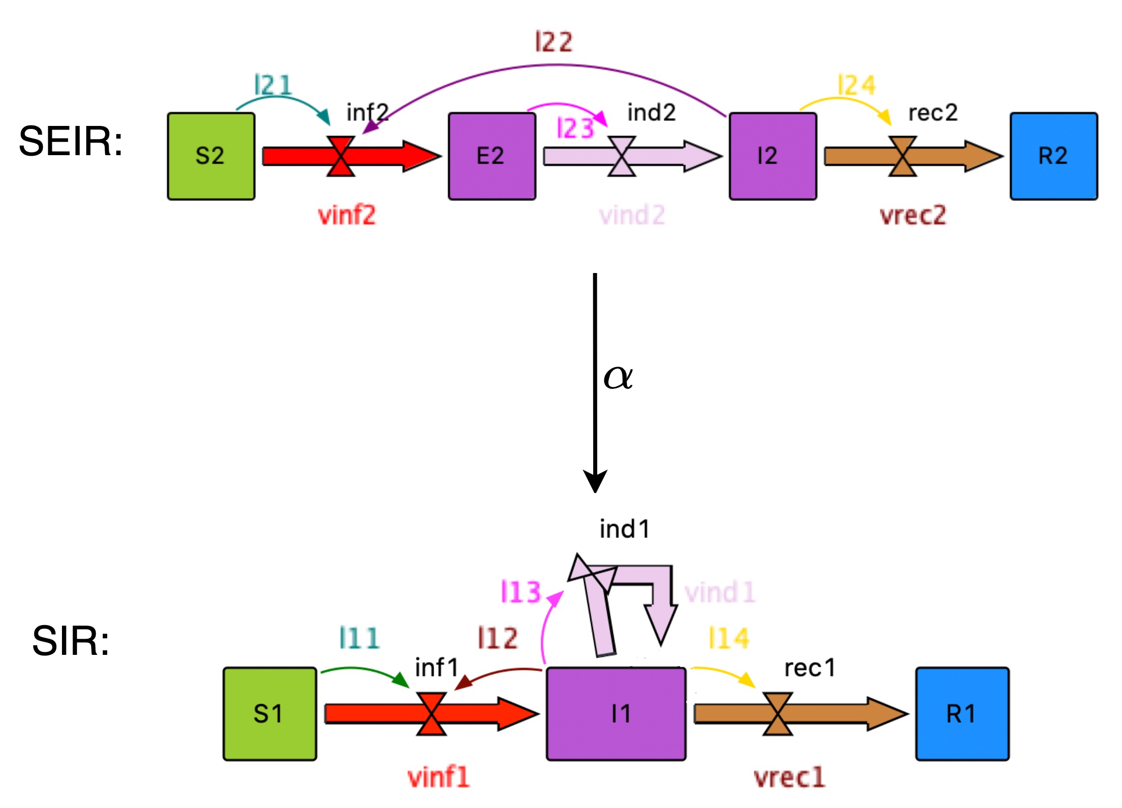
Figure 11: An example of a map (morphism) from the SEIR system structure diagram to the SIR system structure diagram

[width=0.5]juliaCodeAndExamples/s_type.png

Figure 12: A stock-flow diagram $S_{\textrm{type}}$ serving as a type system for infectious disease models

Now let us turn to examples of stratification. Figure 12 shows a system structure diagram $S_{\textrm{type}}$ that can serve as a type system for stratified infectious disease models. This system structure diagram has just one stock, Pop, which represents all the kinds of populations. It has five flows, representing five different types of flows in the infectious disease models we wish to build:

1. the birth flow,

2. the death flow,

3. the flow for new (incident) infections,

4. the aging flow representing the transition from one age group to its immediately older group,

5. the first order delay flow based on the schema of the system structure diagrams.

To support a clearer visualization, these flows are drawn using five different colours. The type system $S_{\textrm{type}}$ has five auxiliary variables corresponding to these five flows—but for simplicity, we do not depict these auxiliary variables. It also has three sum auxiliary variables:

1. $\mathrm{N}$, representing the total population of the whole model,

2. $\mathrm{NS}$, representing the population of a specific subgroup,

3. $\mathrm{NI}$, representing the count of infectious persons of a specific subgroup.

Finally, the type system $S_{\textrm{type}}$ has nine links.

Figure 13 shows four system structure diagrams “typed” by $S_{\textrm{type}}$: that is, equipped with maps to $S_{\textrm{type}}$. The first two are infectious disease models which can serve as aggregate models $S_{\textrm{aggregate}}$: an SEIR model and an SIS (Susceptible–Infectious–Susceptible) model. The second two can serve as strata models $S_{\textrm{strata}}$: a sex strata model and an age strata model. The “typing” of these four stock-flow diagrams—that is, their maps to $S_{\textrm{type}}$—are indicated by colours following the colouring scheme of Figure 12.

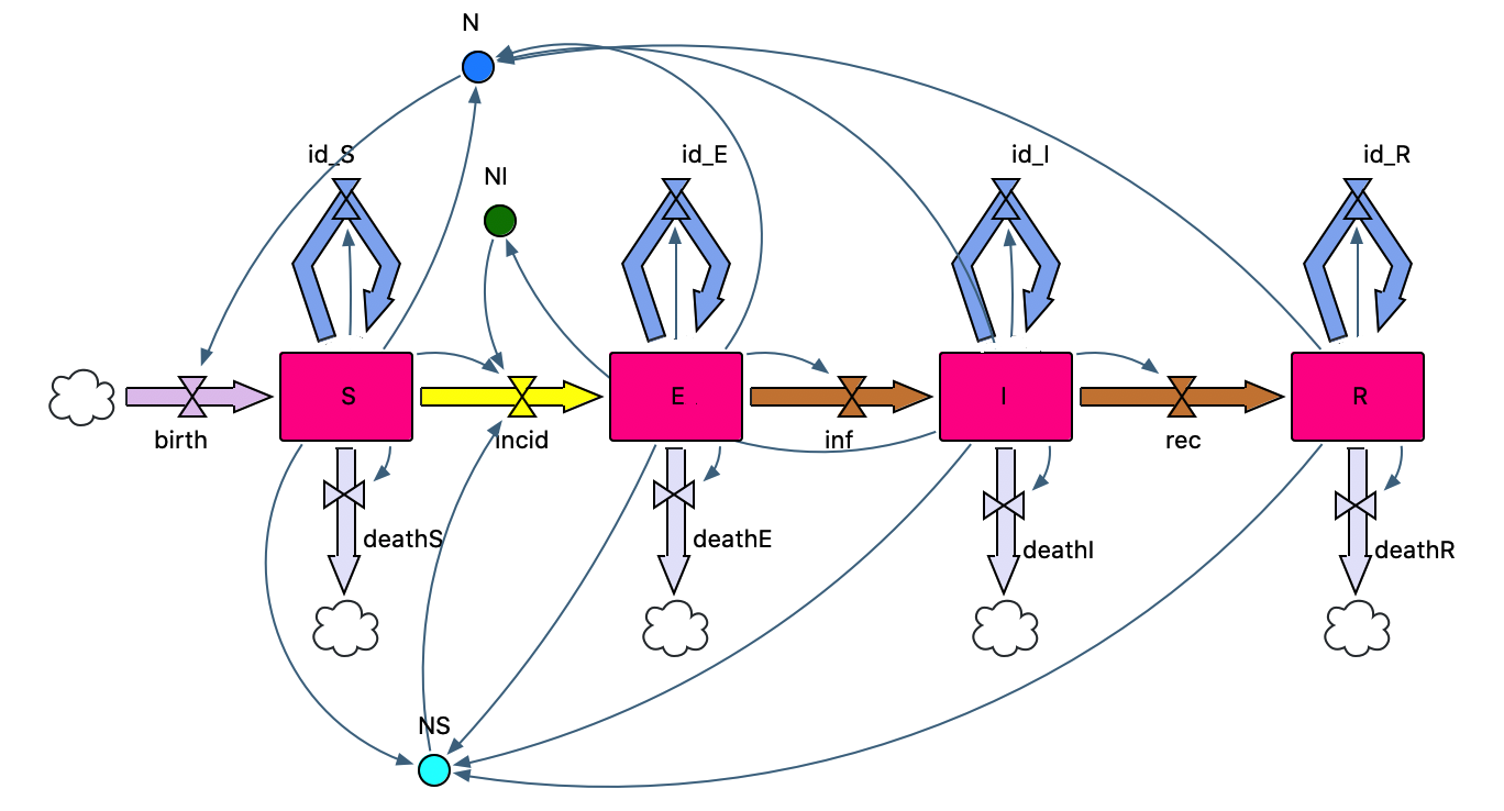
(a) Typed SEIR disease model

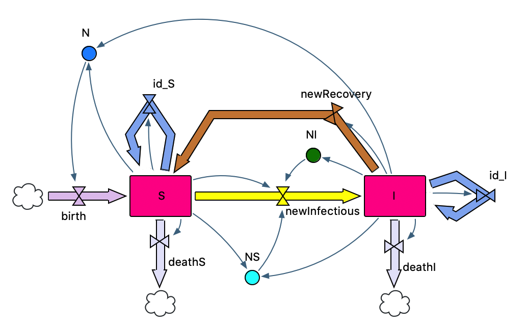
(b) Typed SIS disease model

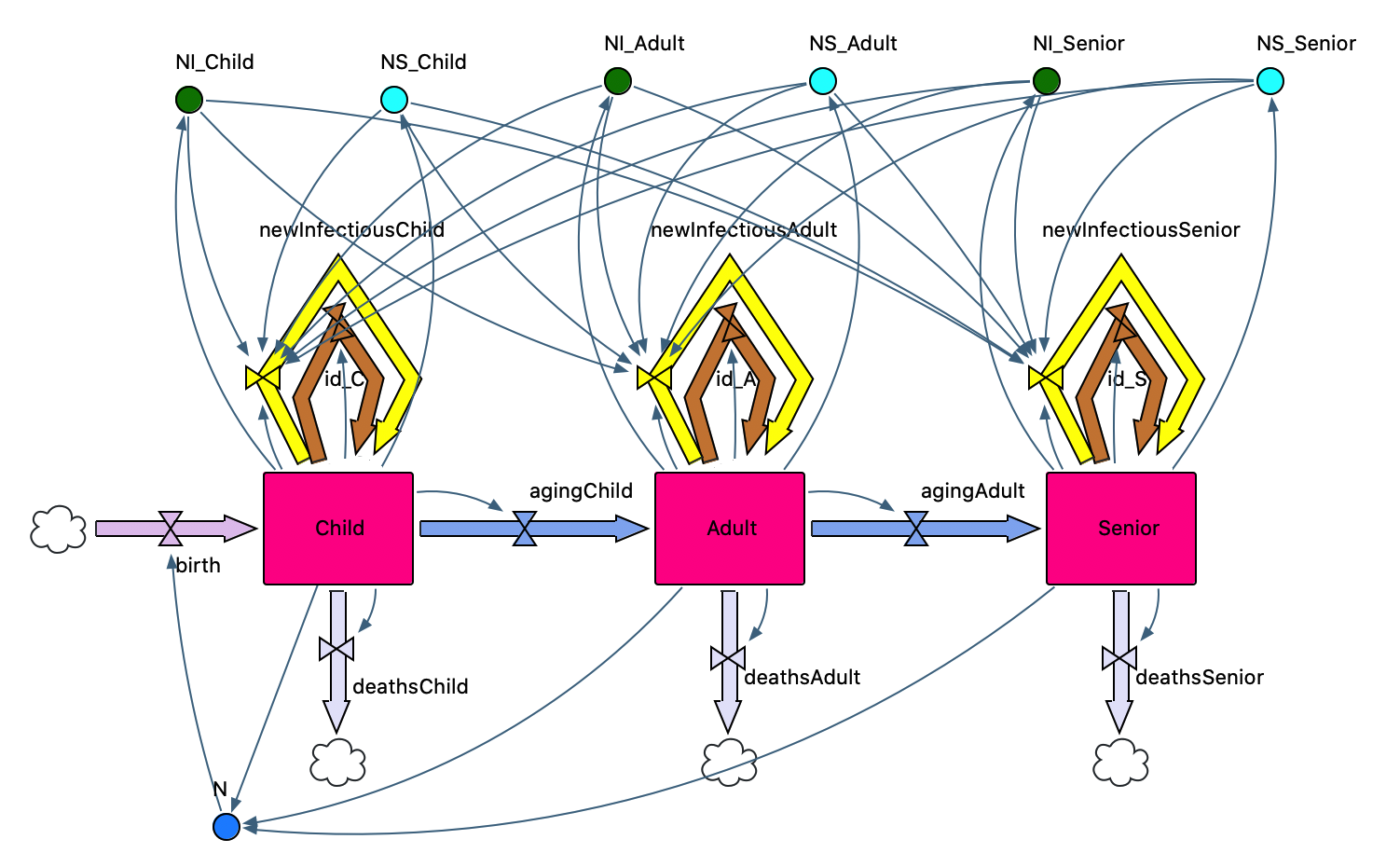
(c) Typed age strata model

(d) Typed sex strata model

Figure 13: Four examples of typed stock-flow diagrams

In Figure 14 we show the results of pullback-based stratification for each combination of an aggregate model (either the SEIR model or SIS model) and a strata model (either the age strata model and sex strata model). A stratified model $S_{\textrm{stratified}}$ is generated by taking the pullback of each of the four combinations of an aggregate model and a strata model. These four stratified models are the age-stratified SEIR model, age-stratified SIS model, sex-stratified SEIR model and sex-stratified SIS model.

More generally, we can define many other system structure diagrams $S_{\textrm{aggregate}}$ to serve as aggregate models for infectious disease anderson1992infectious . Similarly, we can define many different system structure diagrams $S_{\textrm{strata}}$ to serve as strata models characterizing the structure and patterns of progression associated with different types of stratification: not only sex and age but also by socioeconomic or employment status, and geographical stratification including mobility amongst regions, mobility amongst regions from a home base in a particular region, etc. Once an aggregate model and strata model are chosen along with their typings $t_{\textrm{aggregate}}\colon S_{\textrm{aggregate}}\to S_{\textrm{type}}$ and $t_{\textrm{strata}}\colon S_{\textrm{strata}}\to S_{\textrm{type}}$, our code can automatically construct a stratified model by taking a pullback. For example, we can generate an SEIR age-stratified system structure diagram by calculating the pullback of the SEIR model and an age strata model.

Figure 14: Examples of four stratified models

Moreover, we can build stratified models with multiple dimensions by taking repeated pullbacks of multiple stock-flow diagrams. For example, we can build an age-and-sex stratified SEIR model by such an iterated pullback involving strata models for each of two dimensions—sex and age. The result is shown in Figure 15. Similar approaches can be used to model progression of multiple comorbidities and behavioural risk factors—a form of stratification that, done by hand, would be subject to a combinatorial explosion of detail osgood2009Comorbidities .

As mentioned, the stratified models here are built based on system structure diagrams, with the goal of simplifying the stratification process and avoiding the need to consider the functions in the stock-flow diagrams. Fully stratified stock-flow diagrams are then generated by assigning functions to each auxiliary variable of the stratified system structure diagram. Figure 16 shows a solution of an example SIS model stratified by sex.

Figure 15: Example of building an SEIR model stratified in multiple dimensions

[width=0.6]fig/example_stratified_sis_ODEs_solution.jpg

Figure 16: Solutions of the ODE semantics for a sex-stratified SIS model

6 ModelCollab: A Graphical Real-time Collaborative Compositional Modeling Tool

While the modular modeling approaches explored in this chapter make ubiquitous use of category theory, use of the resulting functionality—for example, the ability to compose and stratify diagrams, or to interpret them through differing analyses—does not require knowledge of that foundation. Impactful infectious disease modeling is typically conducted in interdisciplinary teams, and securing timely, ongoing feedback about model structure and emergent behaviour from non-modeler team members is key to both model refinement and organizational learning from modeling. Often tacit knowledge of non-modeling team members concerning the system under study (say, evidence for episodic reemergence of a communicable disease in certain demographic segments despite prevention and control efforts) is only elicited once team members have a chance to comment on visualizations of model structure and summaries of model dynamics. Often interpretation of such dynamics is greatly enhanced through reasoning about the relationship between observed behaviour and the diagram structure – for example, through recognizing that an increase in a variable over time reflects a situation where inflow is greater than outflow, explaining an invariant value of a state variable in terms of a balance between inflows and outflows, or reasoning about exponential change in terms of driving feedback loops.

Partly for these reasons, the System Dynamics tradition of modeling has long prized the use of visual modeling software that keeps the attention of modelers – and other team members – on diagrams depicting model structure. While such software does support communication across interdisciplinary team members, it sufferings both from the disadvantages of traditional treatment of such models discussed in the introduction and a limit to being modified—and often viewed—by only a single user at a time.

We describe here open-source, visual, collaborative, categorically-rooted, diagram-centric software for building, manipulating, composing, and analyzing System Dynamics models. This web-based software, named ModelCollab, is designed for real-time collaborative use across interdisciplinary teams. The graphical user interface allows the user to interactively conduct the types of categorically-rooted operations discussed without any knowledge of their categorical foundations. This software is at an early stage, and currently supports only a subset of the options made possible by the StockFlow.jl framework on which it rests. But its development is progressing rapidly, and we anticipate an expansion to eventually handle a far larger set of operations. We describe use of some of the early features of this system, bearing in mind that multiple users will commonly be using the system simultaneously.

ModelCollab provides a modal interface for adding diagram components to a Canvas used to display the diagram being assembled. Different concurrent users can be present in different modes at the same time. For example, within “Stock” mode, the user can click on the canvas to add a Stock, and similarly for “Flow”, “Auxiliary Variable”, “Sum Variable” modes. “Connect” mode is used to establish links indicating dependencies, such as those for auxiliary and sum variables. The interface abstraction level sometimes exceeds that of StockFlow.jl; for example, flows within the graphical interface are shown as depending directly on other variables in the diagram, rather than only via connections with a distinct auxiliary variable. Through this interface, larger diagrams can be created; for example, Figure 17 depicts an SEIR diagram built in the system.

Figure 17: An SEIR diagram built in ModelCollab

As in online collaborative software such as Google Docs, diagrams can be accessed on an ongoing basis by multiple parties once they have been created in ModelCollab. It is also possible to persist diagrams in other forms within the system. The interface allows export of diagrams through a menu item, with that diagram then being downloaded to the invoking user’s local computer as a JSON json file. Beyond exporting, the system offers a structured means of “publishing” diagrams to a simple “Diagram Library” once they have attained a sufficient level of maturity to be worth sharing. Such published diagrams can then be reused by others.

A foundationally important component of ModelCollab functionality is the ability to compose diagrams. Like other diagram assembly operations within ModelCollab, this operation is performed graphically. As a first step, the user can add previously published diagrams into the model canvas, where this imported diagram (henceforth referred to as the “subdiagram”) is visually distinguished from the surrounding diagram being assembled, as is depicted in 18.

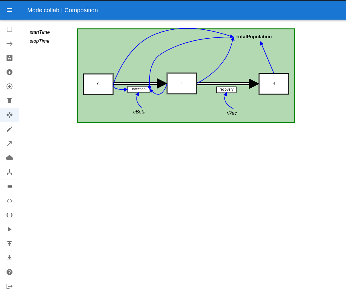
Figure 18: ModelCollab: Results of importing a single previously published diagram

More than one such published diagram can be imported, in which case each is distinguished by a different colour. For example, Figure 19 shows the results of importing a second subdiagram, which lies beneath the first imported subdiagram. Beyond these subdiagrams, the canvas will commonly contain a surrounding diagram.

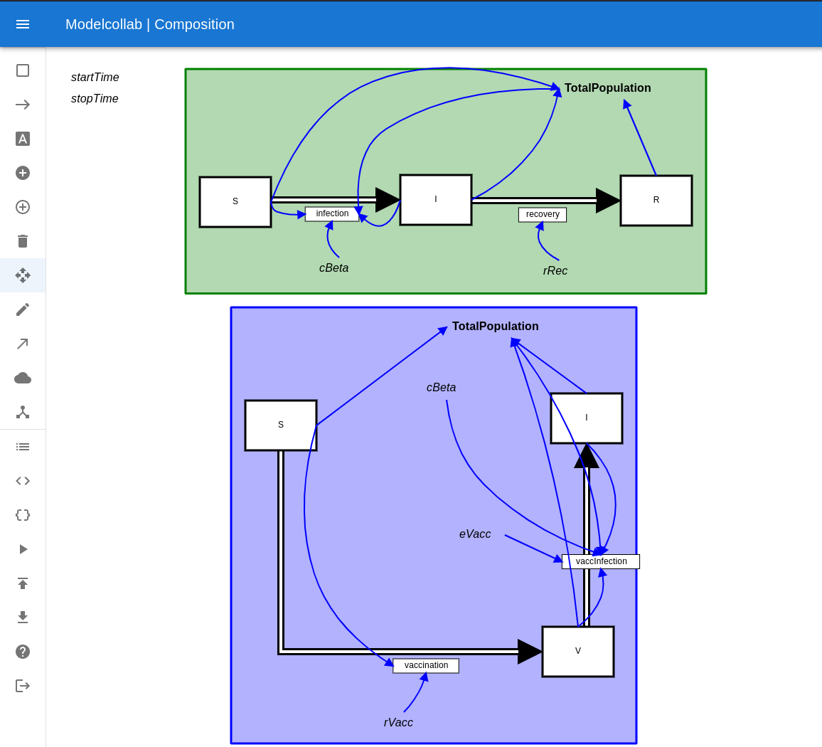
Figure 19: ModelCollab: Results of importing a second diagram

Just after being imported, the two subdiagrams are independent of one another; while this is sometimes appropriate, often the user will recognize ways in which the process depicted in a specific imported subdiagram is coupled with the processes depicted by the surrounding diagram, or in the other imported subdiagrams. Such coupling is represented by composition of the diagrams via the interface. Through user interface actions, a user can elect to identify (unify) a stock or sum dynamic variable with a variable of the same type in a subdiagram. Such identification of pairs of variables may be performed between variables in an outer canvas diagram and in a subdiagram, or (alternatively) between two variables in different subdiagrams. For example, 20 graphically illustrates the results of identification of a stock V of the upper and lower diagrams. By entering “Identify” mode from the ModelCollab menu, the user can indicate with a pair of successive clicks the pair of stocks to be identified.

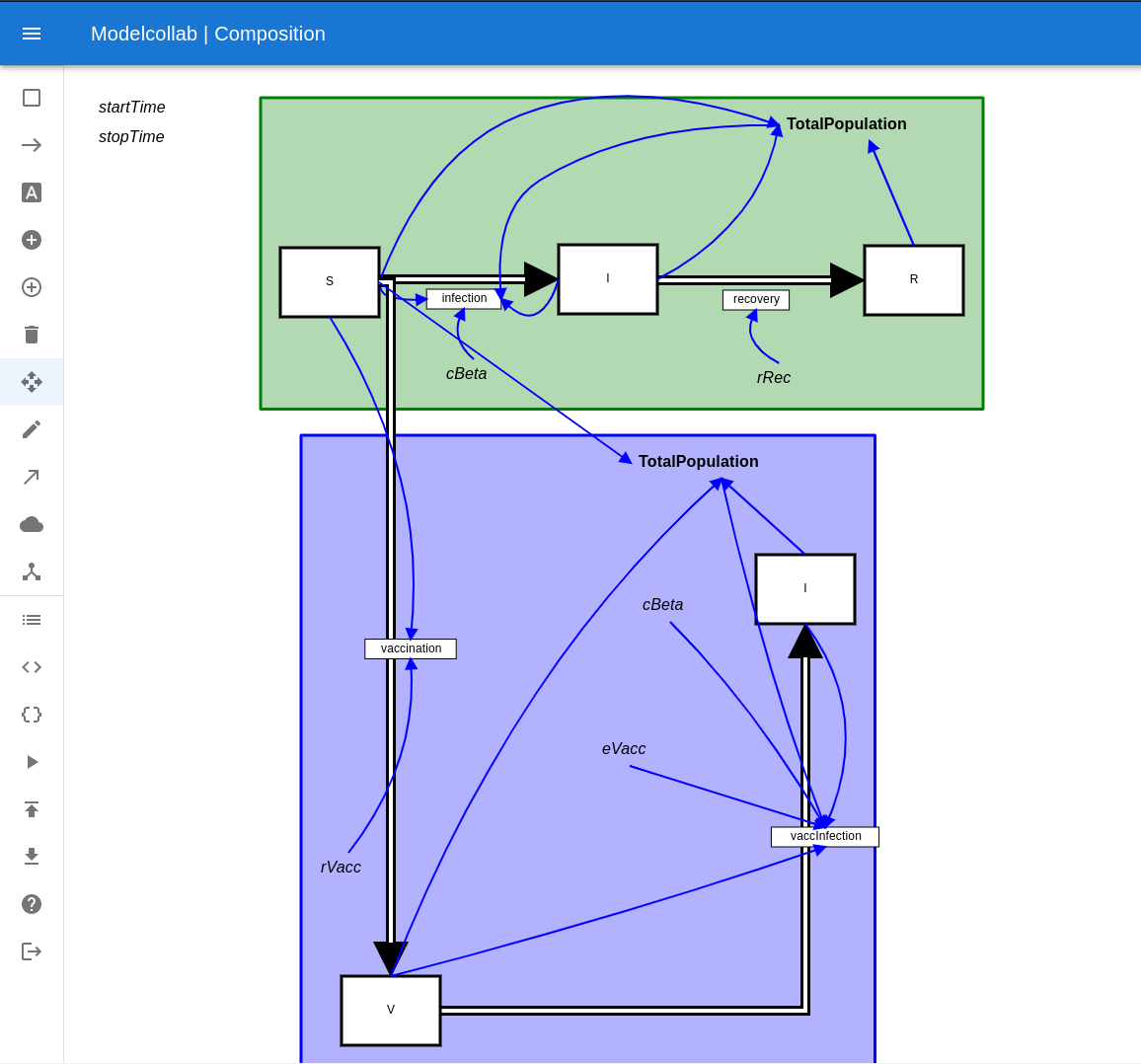
Figure 20: ModelCollab: Example of two subdiagrams composed by identifying stock S

Figure 21 shows the results of using the “Identify” mode of ModelCollab to identify not just additional stock I between the two diagrams, but also sum variable N.

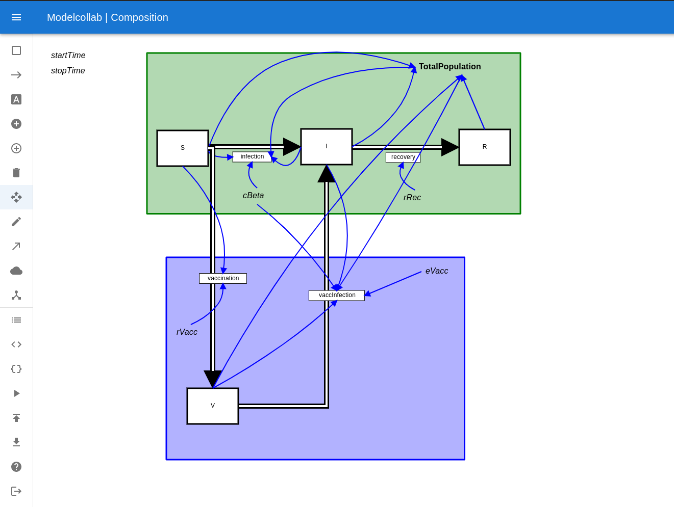
Figure 21: ModelCollab: Example of two subdiagrams composed by identifying both stocks S and I and sum variable N

Once built, ModelCollab supports rendering the definition of a diagram in code form. Specifically, the system offers a “Get code” menu item that produces a file containing Julia code to create the current diagram using calls to StockFlow.jl. If desired, such code could then be used to interactively manipulate the models from a Julia codebase or within a Jupyter notebook.

Beyond operating on syntactic constructs in the form of diagrams, ModelCollab provides an interface to interpret diagrams according to a menu-chosen semantics. At the time of writing, the software only supports ODE semantics (see Figure 22), but implementation of the other semantics discussed in section 3 is planned within the near future.

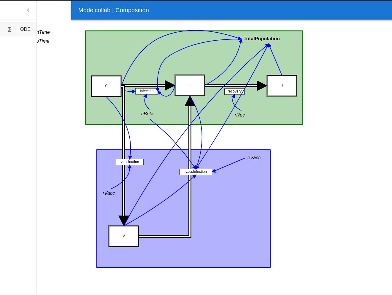
Figure 22: ModelCollab: Example of using the “Semantics” menu to elect to interpret the diagram (the syntax) as an ODE

Interpretation of a diagram by ODE semantics involves numerical integration of that diagram over a user-specified timeframe. Outputs from that simulation are currently rendered and downloaded as a PNG image file; Figure 23 shows an example.

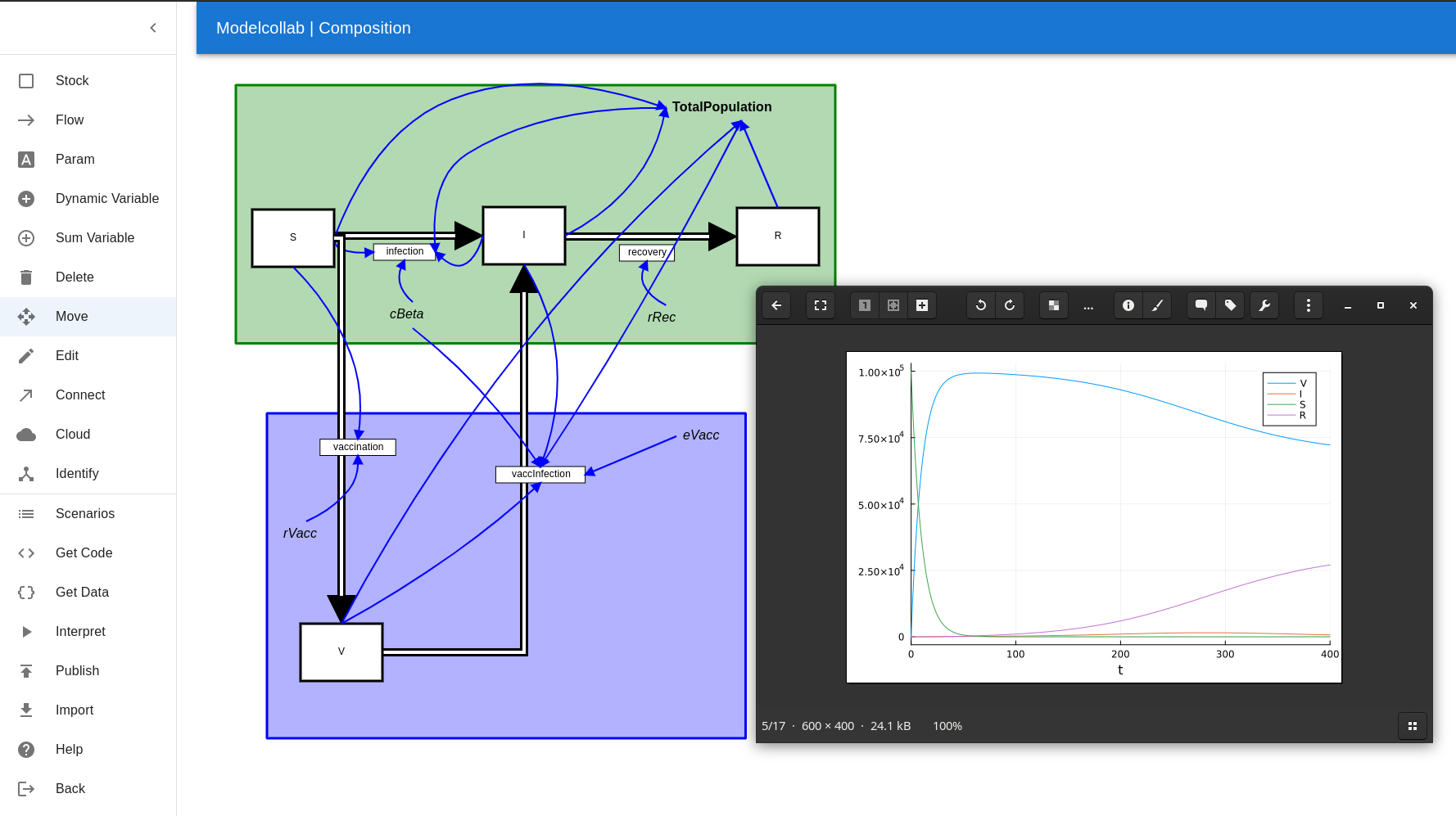
Figure 23: ModelCollab: Example of results of interpreting the composed diagrams (the syntax) with ODE semantics

The current ModelCollab software represents a modest step towards realizing the promise of compositional approaches for the broader modeling community. There are several priorities anticipated for rollout in the near future. Putting aside additions requiring changes for StockFlow.jl itself (some of which are discussed below), planned features include support for pullback-based stratification and additional semantic domains. Furthermore, a scenario-based interface is being planned that will provide persistent options to interpret the model using different semantics and settings, and support other users in observing and annotating the output from semantic-based interpretation long after it is first produced. Support is also planned for the type of seamless version control standard in many real-time collaborative systems and indications of the presence of the pointers of different concurrent users. Finally, role-based security, authentication and authorization systems are planned to formalize permission-based enablement of diagram use, sharing and modes of interaction.

7 Conclusion

This chapter demonstrates some of the modeling benefits secured when one takes diagrams seriously. Specifically, we have offered a brief look at some of the characteristics of categorical treatment of stock-flow diagrams, while offering a nod to other related diagrams within the diagram-centric System Dynamics modeling tradition. While our treatment has been informal and has only touched on a small subset of the consequences of a categorical foundation for diagrams, we have highlighted several benefits: the capacity to promote modularity and reuse via diagram composition, to sidestep model opacity arising from the curse of dimensionality afflicting stratified models via a modular stratification, and better supporting the needs of interdisciplinary stakeholders via the capacity to interpret the same diagrams through the lens of varying semantic domains. Some of these benefits—such as those involving semantics mapping stock-flow diagrams to system structure diagrams or causal loop diagrams—describe relationships between different types of diagrams not previously formalized. Other outcomes of providing a firm mathematical basis for stock-flow models have been noted in passing. For example, such a formalization offers the ability to soundly transform a diagram whilst maintaining invariant its mathematical meaning, such as for optimization or parallelization of model simulation. As another example, the formalization can also allow the use of maps between diagrams that coarse-grain model structure. There are diverse other opportunities for exploiting this categorical formalization of mathematical structure.

While it offers promise, this work remains at the earliest stages of exploiting such opportunities extending from categorifying stock-flow diagrams. StockFlow.jl and ModelCollab require many important extensions to substantively address the challenges of practical modeling. Key priorities include providing support for upstream/downstream composition based on “half-edge” flows emerging from a diagram, supporting methods for hierarchical composition of diagrams (such as those pioneered by our colleague N. Meadows NicholasHierarchicalCEPHILTechReport2022 ), adding full support for causal loop diagrams and system structure diagrams, and supporting the augmentation of multiple types of diagrams with dimensional information hart1995multidimensional and use of such information in stock-flow diagram composition, stratification and additional semantic domains. There is further a need and opportunity to develop additional semantic domains for use with stock-flow models. These include those associated with different numerical simulations, such as stochastic transition systems, stochastic differential equations and difference equations, as well as those associated with computational statistics techniques. We seek to follow each such advance in the formalisms for stock-flow models by successive implementation in StockFlow.jl and ModelCollab.

At a time where health dynamic modeling is in greater demand and more needed than ever, formalizing its categorical foundation confers benefits key to addressing the team-based modeling needs of the 21st century. We enthusiastically welcome collaboration with colleagues interested in exploring opportunities to transformationally enable health modeling by tapping the power of category theory.

See pages - of codeAndExamples.pdf