Multicast Beamformer Design
for MIMO Coded Caching Systems

Abstract

Coded caching (CC) techniques have been shown to be conveniently applicable in multi-input multi-output (MIMO) systems. In a $K$-user network with spatial multiplexing gains of $L$ at the transmitter and $G$ at every receiver, if each user can cache a fraction $\gamma$ of the file library, a total number of $GK\gamma+L$ data streams can be served in parallel. In this paper, we focus on improving the finite-SNR performance of MIMO-CC systems. We first consider a MIMO-CC scheme that relies only on unicasting individual data streams, and then, introduce a decomposition strategy to design a new scheme that delivers the same data streams through multicasting of $G$ parallel codewords. We discuss how optimized beamformers could be designed for each scheme and use numerical simulations to compare their finite-SNR performance. It is shown that while both schemes serve the same number of streams, multicasting provides notable performance improvements. This is because, with multicasting, transmission vectors are built with fewer beamformers, leading to more efficient usage of available power resources.

I Introduction

Wireless communication networks are under mounting pressure to support exponentially increasing volumes of multimedia content [1] and to provide the infrastructure for the imminent emergence of new applications such as wireless immersive viewing [2, 3]. For the efficient delivery of such multimedia content, the work of Maddah-Ali and Niesen in [4] proposed the idea of coded caching (CC) as a means of increasing the data rates by exploiting cache content across the network. In a single-stream downlink network of $K$ users each with a cache memory large enough to store a portion $\gamma\leq 1$ of the entire file library, CC enables boosting the achievable rate by a factor of $K\gamma+1$. This is achieved by multicasting carefully created codewords such that each user can use its cache content to remove unwanted parts from the received signal. As a result, with CC, the achievable DoF is increased from one to $K\gamma+1$. The multiplicative factor $t\equiv K\gamma$ is also called the coded caching gain.

Motivated by the growing importance of multi-antenna wireless communications [5], the authors in [6, 7] explored the cache-aided MISO setting, revealing that for a downlink MISO setup with cache-enabled users and the transmitter-side multiplexing gain of $L$, the cumulative DoF of $t+L$ is achievable. Many subsequent works then explored various implementation challenges of MISO-CC schemes, including but not limited to, optimal beamformer design [8, 9, 10], exponentially growing subpacketization [11, 12], and applicability to dynamic setups [13, 14].

Compared to MISO setups, applying CC techniques in MIMO communications has been less investigated. In [15, 16], information-theoretic approaches were used to find upper bounds to the achievable DoF in MIMO-CC setups with multiple transmitters and receivers. It was revealed that multiple antennas at the receiver side could actually increase the DoF over MISO settings. Following the same direction, the authors in [17] proposed a low-complexity solution to construct MIMO-CC schemes building on any given scheme available for MISO setups. It was shown that for the simple case of a MIMO setting with a single transmitter and multiple receivers with spatial multiplexing gains of $L$ and $G$, respectively, if $\frac{L}{G}$ is an integer, the cumulative DoF of $Gt+L$ is achievable. In other words, multiple receive antennas enable a multiplicative boost in the coded caching gain.

In this paper, we study the finite-SNR performance of MIMO-CC schemes. We start with the scheme in [17], which is based on unicasting individual data terms, and explain how optimized beamformers could be designed for this scheme following a similar approach to [8]. Then, we discuss how the underlying MIMO structure could be used to decompose the system into multiple parallel MISO setups (or single-antenna, if $L=G$), and how this decomposition could enable transmitting several multicast codewords simultaneously. While both considered schemes deliver the same number of streams in each transmission, we expect the scheme with multicasting to have better performance in the finite-SNR regime as it requires fewer beamformers in each transmission (hence, the usage of available power resources is more efficient). Finally, numerical simulations are used to verify this assumption.

Throughout the text, we use the following notations. For integer $J$, $[J]$ is the set of numbers $\{1,2,\cdot\cdot\cdot,J\}$. Boldface upper- and lower-case letters indicate matrices and vectors, respectively, and calligraphic letters denote sets. For two sets ${\mathcal{K}}$ and ${\mathcal{T}}$, ${\mathcal{K}}\backslash{\mathcal{T}}$ is the set of elements in ${\mathcal{K}}$ that are not in ${\mathcal{T}}$. Other notations are defined as they are used in the text.

II System Model

We consider a MIMO communication setup with $K$ users, ${\mathsf{L}}$ antennas at the transmitter, and ${\mathsf{G}}$ antennas at each receiver. We assume the spatial multiplexing gains at the transmitter and receivers are set to $L\leq{\mathsf{L}}$ and $G\leq{\mathsf{G}}$, i.e., the transmitter can deliver $L$ data streams and each user can receive $G$ data streams simultaneously. This requires that the channel matrices ${\mathbf{H}}_{k}\in\mathbb{C}^{{\mathsf{G}}\times{\mathsf{L}}}$ from the transmitter to every user $k\in[K]$ to have ranks not smaller than $G$, and the cumulative channel matrix formed by the vertical concatenation of individual channel matrices as ${\mathbf{H}}=[{\mathbf{H}}_{1}^{H};{\mathbf{H}}_{2}^{H};\cdots;{\mathbf{H}}_{k}^{H}]^{H}$ to have a rank larger than or equal to $L$. Each user has a cache memory of size $MF$ bits, and requests files from a library ${\mathcal{F}}$ of $N$ files each with size $F$ bits. For notational simplicity, we use a normalized data unit and ignore $F$ in subsequent notations. The coded caching gain is defined as $t\equiv\frac{KM}{N}$ and indicates how many copies of the file library can be stored in the cache memories of all the users. We assume both $\eta\equiv\frac{L}{G}$ and $t$ are integers.

The system operation consists of two phases; placement, and delivery. In the placement phase, users’ cache memories are filled up with data. Following a similar structure as in [7], we split each file $W\in{\mathcal{F}}$ into $\binom{K}{t}$ subfiles $W_{{\mathcal{P}}}$, where ${\mathcal{P}}\subseteq[K]$ can be any subset of users with $|{\mathcal{P}}|=t$. Then, in the cache memory of user $k\in[K]$, we store $W_{{\mathcal{P}}}$, $\forall W\in{\mathcal{F}}$, $\forall{\mathcal{P}}:k\in{\mathcal{P}}$.

At the beginning of the delivery phase, every user $k$ announces its requested file $W(k)\in{\mathcal{F}}$ to the server. The server then builds and transmits a vector ${\mathbf{x}}({\mathcal{K}})$ for every subset of users ${\mathcal{K}}\subseteq[K]$ with $|{\mathcal{K}}|=t+\eta$ (transmissions are done, e.g., in consecutive TDMA slots). Each ${\mathbf{x}}({\mathcal{K}})$ is built to deliver $G$ parallel data streams to every user in ${\mathcal{K}}$, resulting in the total DoF of $G(t+\eta)=Gt+L$. After transmitting ${\mathbf{x}}({\mathcal{K}})$, every user $k\in{\mathcal{K}}$ receives ${\mathbf{y}}_{k}({\mathcal{K}})={\mathbf{H}}_{k}{\mathbf{x}}({\mathcal{K}})+{\mathbf{z}}_{k}$, where ${\mathbf{z}}_{k}\in\mathbb{C}^{{\mathsf{G}}\times 1}$ is the additive white Gaussian noise (AWGN) with power $N_{0}$. Then, receive beamforming vectors ${\mathbf{u}}_{k,g}\in\mathbb{C}^{{\mathsf{G}}\times 1}$, $g\in[G]$ are used to produce stream-specific received signals $y_{k,g}({\mathcal{K}})={\mathbf{u}}_{k,g}^{H}{\mathbf{y}}_{k}({\mathcal{K}})$. For simplicity, let us use ${\mathsf{s}}_{k,g}$ to denote the stream $g$ at user $k$, and define the equivalent channel vector for the stream ${\mathsf{s}}_{k,g}$ as ${\mathbf{h}}_{k,g}=({\mathbf{u}}_{k,g}^{H}{\mathbf{H}}_{k})^{H}$. Then, we have

$$y_{k,g}({\mathcal{K}})={\mathbf{h}}_{k,g}^{H}{\mathbf{x}}({\mathcal{K}})+z_{k,g}\;,$$ (1)

where $z_{k,g}={\mathbf{u}}_{k,g}^{H}{\mathbf{z}}_{k}$ denotes the AWGN over the stream ${\mathsf{s}}_{k,g}$.

The transmission vectors ${\mathbf{x}}({\mathcal{K}})$ are built using the delivery algorithm of the considered MIMO-CC scheme. In this paper, we study two schemes with the same number of parallel data streams but with different transmission strategies; unicasting and multicasting. The details of the schemes are provided in subsequent sections.

III Data Delivery with Unicasting

For data delivery with unicasting, we consider the MISO scheme in [7] as the baseline and use the stretching mechanism in [17] to apply it to MIMO setups. As a result, we first split every subfile $W_{{\mathcal{P}}}$ into $Q=\binom{K-t-1}{L-1}$ smaller parts $W_{{\mathcal{P}}}^{q}$, $q\in[Q]$, and then, split every resulting part $W_{{\mathcal{P}}}^{q}$ into $G$ subpackets $W_{{\mathcal{P}}}^{q,g}$, $g\in[G]$. The index $q$ does not affect our analysis in this paper and is removed for notational simplicity. Then, the transmission vector ${\mathbf{x}}({\mathcal{K}})$ is built as

$${\mathbf{x}}({\mathcal{K}})=\sum_{\begin{subarray}{c}{\mathcal{T}}\subseteq{\mathcal{K}}\\ |{\mathcal{T}}|=t+1\end{subarray}}\sum_{\begin{subarray}{c}k\in{\mathcal{T}}\end{subarray}}\sum_{G\in[G]}W_{{\mathcal{T}}\backslash\{k\}}^{g}(k){\mathbf{w}}_{{\mathcal{R}}({\mathcal{K}},{\mathcal{T}},k,g)}\;,$$ (2)

where

$${\mathcal{R}}({\mathcal{K}},{\mathcal{T}},k,g)=\bigcup_{\begin{subarray}{c}\bar{k}\in{\mathcal{K}}\backslash{\mathcal{T}}\\ \bar{g}\in[G]\end{subarray}}\{{\mathsf{s}}_{\bar{k},\bar{g}}\}\;\bigcup_{\begin{subarray}{c}\bar{g}\in[G]\backslash\{g\}\end{subarray}}\{{\mathsf{s}}_{k,\bar{g}}\}$$ (3)

represents the set of streams over which the interference is suppressed by beamforming, and ${\mathbf{w}}_{{\mathcal{R}}(\cdot)}$ denotes transmit beamformers. As a quick explanation, using vector ${\mathbf{x}}({\mathcal{K}})$, we transmit $G(t+1)\binom{t+\eta}{t+1}$ subpackets (recall that $|{\mathcal{K}}|=t+\eta$), and all these subpackets can be decoded simultaneously as the interference caused by each of them over other streams is either suppressed by beamforming or could be reconstructed and removed using the cache contents. The following example clarifies this procedure.

Example 1.

Consider a MIMO setup where spatial multiplexing gains at the transmitter and receivers are $L=G=2$, and the coded caching gain is $t=1$ (i.e., $t+\eta=2$). Let us consider the transmission vector serving users 1 and 2, assuming they have requested files $A$ and $B$, respectively. It is built as

$${\mathbf{x}}(\{1,2\})=A_{2}^{1}{\mathbf{w}}_{{\mathsf{s}}_{1,2}}+A_{2}^{2}{\mathbf{w}}_{{\mathsf{s}}_{1,1}}+B_{1}^{1}{\mathbf{w}}_{{\mathsf{s}}_{2,2}}+B_{1}^{2}{\mathbf{w}}_{{\mathsf{s}}_{2,1}}\;,$$ (4)

and delivers four subpackets to users 1 and 2 in parallel (note that the brackets for sets ${\mathcal{R}}(\cdot)$ are removed for notational simplicity). Let us review the decoding process for the first subpacket for user 1, i.e., $A_{2}^{1}$. Using (1), the respective stream-specific received signal for this subpacket is

$$y_{1,1}(\{1,2\}) ={\mathbf{h}}_{1,1}^{H}{\mathbf{x}}(\{1,2\})+z_{1,1}$$

$$=A_{2}^{1}{\mathbf{h}}_{1,1}^{H}{\mathbf{w}}_{{\mathsf{s}}_{1,2}}+A_{2}^{2}{\mathbf{h}}_{1,1}^{H}{\mathbf{w}}_{{\mathsf{s}}_{1,1}}+I_{c}+z_{1,1},$$

where the interference term $I_{c}=B_{1}^{1}{\mathbf{h}}_{1,1}^{H}{\mathbf{w}}_{{\mathsf{s}}_{2,2}}+B_{1}^{2}{\mathbf{h}}_{1,1}^{H}{\mathbf{w}}_{{\mathsf{s}}_{2,1}}$ can be fully reconstructed and removed using the cache contents of user 1. Now, by definition, the remaining interference term $A_{2}^{2}{\mathbf{h}}_{1,1}^{H}{\mathbf{w}}_{{\mathsf{s}}_{1,1}}$ is also suppressed by beamforming, and hence, $A_{2}^{1}$ is decodable at user 1. Following the same process, all the other three streams could also be decoded successfully.

In [17], zero-force (ZF) unicast beamformers are used to completely null out the interference, i.e., transmit and receive beamformers are built such that ${\mathbf{h}}_{k,g}^{H}{\mathbf{w}}_{{\mathcal{R}}({\mathcal{K}},{\mathcal{T}},k,g)}=0$ for every ${\mathsf{s}}_{k,g}\in{\mathcal{R}}({\mathcal{K}},{\mathcal{T}},k,g)$. Of course, ZF beamforming is not an appropriate choice in finite-SNR [8], and we need to design optimized beamformers to improve the performance in this regime. This can be done using alternating optimization together with the successive convex approximation (SCA) method in [8]. To do so, at each step, we fix either transmit or receive beamformers to their latest known values and find the optimal solution for the other one, and update this procedure until the convergence is achieved.

Here, due to lack of space, we review the beamformer design process only for the symmetric case of $L=G$ (i.e., $\eta=1$) and leave the general formulation for the extended version of this paper. The reason for this assumption is that if $\eta>1$, each receiver has to decode multiple subpackets over each stream through an equivalent user-specific multiple access channel (MAC) [8], and hence, linear MMSE receivers would no longer work. However, if $\eta=1$, after solving for optimal transmit beamformers, receive beamformers can be simply calculated as

$${\mathbf{u}}_{k,g}=({\mathbf{H}}_{k}{\mathbf{W}}_{k}{\mathbf{W}}_{k}^{H}{\mathbf{H}}_{k}^{H}+N_{0}{\mathbf{I}})^{-1}{\mathbf{H}}_{k}{\mathbf{w}}_{{\mathcal{R}}({\mathcal{K}},{\mathcal{K}},k,g)}\;,$$ (5)

where ${\mathbf{W}}_{k}\equiv[{\mathbf{w}}_{{\mathcal{R}}({\mathcal{K}},{\mathcal{K}},k,1)};...;{\mathbf{w}}_{{\mathcal{R}}({\mathcal{K}},{\mathcal{K}},k,G)}]$ is formed by concatenating all the $G$ transmit beamformers used to send data to user $k$ (note that when $\eta=1$, ${\mathcal{T}}={\mathcal{K}}$).

Now, assuming receive beamformers are fixed, to calculate optimal transmit beamformers we first notice that the SINR for decoding subpacket $W_{{\mathcal{T}}\backslash\{k\}}^{g}(k)$ at user $k\in{\mathcal{K}}$ is given as

$$\lambda_{k,g}=\frac{|{\mathbf{h}}_{k,g}^{H}{\mathbf{w}}_{{\mathcal{R}}({\mathcal{K}},{\mathcal{K}},k,g)}|^{2}}{\sum_{\begin{subarray}{c}\bar{g}\in[G]\backslash\{g\}\end{subarray}}|{\mathbf{h}}_{k,g}^{H}{\mathbf{w}}_{{\mathcal{R}}({\mathcal{K}},{\mathcal{K}},k,\bar{g})}|^{2}+N_{0}}$$ (6)

and the rate optimization problem will be

$$\max_{{\mathbf{w}}_{{\mathcal{R}}({\mathcal{K}},{\mathcal{K}},k,g)}}\min_{k\in{\mathcal{K}},g\in[G]}r_{k,g}$$ (7)

$$s.t.\quad r_{k,g}\leq\log(1+\lambda_{k,g}),\;\forall k\in{\mathcal{K}},g\in[G]\;,$$

$$\quad\quad\sum_{k\in{\mathcal{K}}}\sum_{g\in[G]}|{\mathbf{w}}_{{{\mathcal{R}}({\mathcal{K}},{\mathcal{K}},k,g)}}|^{2}\leq P_{T}\;,$$

where $P_{T}$ is the total available transmit power. As discussed in [8], this optimization problem is non-convex and can be solved, e.g. using an SCA method similar to [8].

IV Data Delivery with Multicasting

The primary goal of using multicast transmissions in the MIMO-CC scheme is to improve the finite-SNR performance. This is because, with multicasting, fewer beamforming vectors are needed for the transmission, and as a result, the average power allocated to each beamformer is increased. Of course, this will have a more prominent effect in finite-SNR communications as the rate is power-limited in this regime. Similar results for MISO setups could be found in [18, 19].

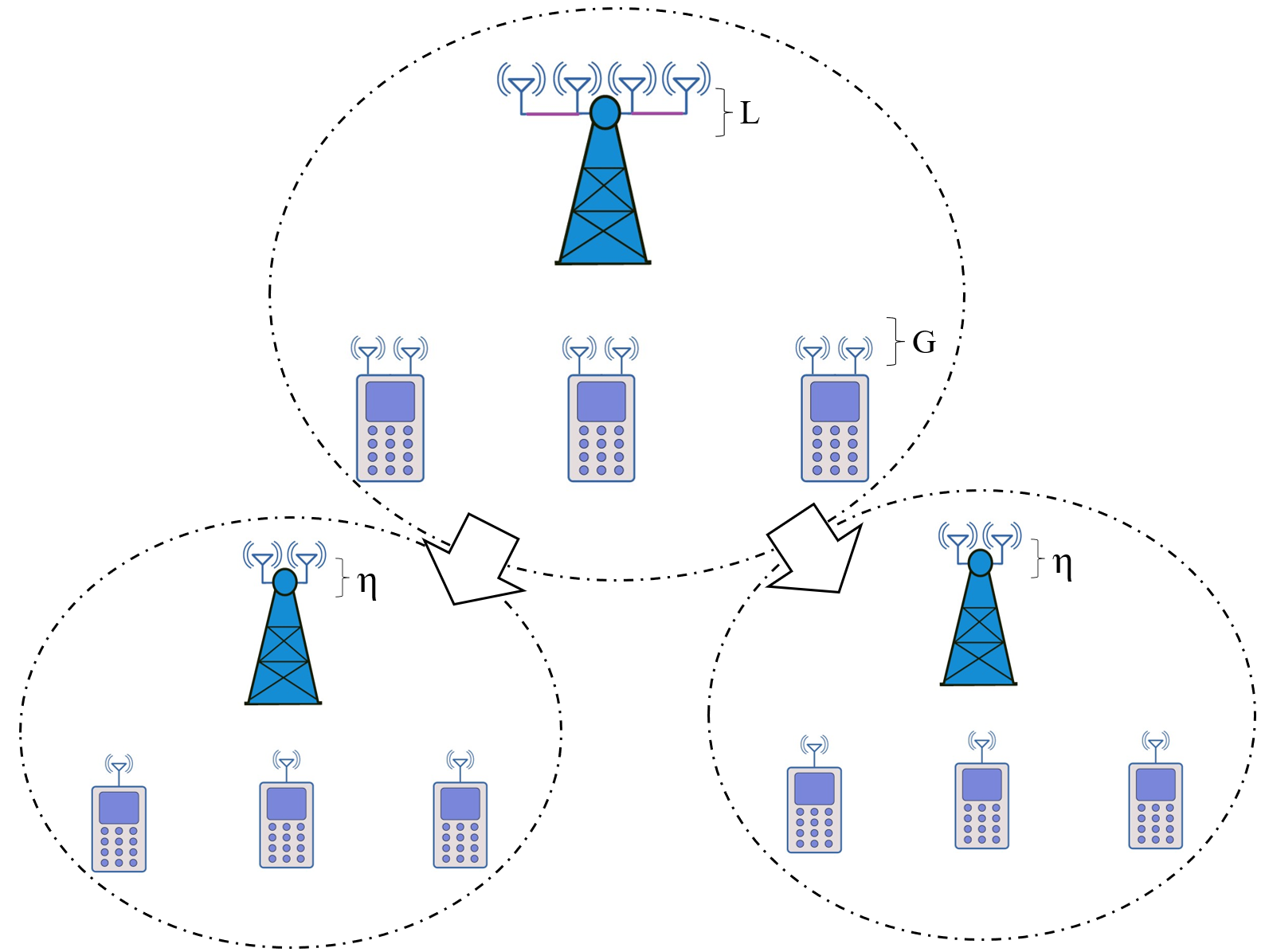
Figure 1: MIMO system decomposition into parallel MISO systems

In order to illustrate the multicasting opportunities available in MIMO-CC, we decompose the MIMO system into $G$ parallel MISO systems (or single-antenna, if $L=G$), as shown in Figure 1. This requires splitting subfiles $W_{{\mathcal{P}}}$ into subpackets $W_{{\mathcal{P}}}^{q,g}$ following the same process as in Section III, and building the multicast-enabled transmission vector $\hat{{\mathbf{x}}}({\mathcal{K}})$ as

$$\hat{{\mathbf{x}}}({\mathcal{K}})=\sum_{\begin{subarray}{c}{\mathcal{T}}\subseteq{\mathcal{K}}\\ |{\mathcal{T}}|=t+1\end{subarray}}\sum_{\begin{subarray}{c}g\in[G]\end{subarray}}{\mathsf{X}}_{{\mathcal{T}}}^{g}\hat{{\mathbf{w}}}_{\hat{{\mathcal{R}}}({\mathcal{K}},{\mathcal{T}},g)}\;,$$ (8)

where, using $\oplus$ to represent the bit-wise XOR operation in the finite field, we have

$${\mathsf{X}}_{{\mathcal{T}}}^{g}=\bigoplus_{k\in{\mathcal{T}}}W_{{\mathcal{T}}\backslash\{k\}}^{g}(k)\;,$$ (9)

$$\hat{{\mathcal{R}}}({\mathcal{K}},{\mathcal{T}},g)=\bigcup_{\begin{subarray}{c}\bar{k}\in{\mathcal{K}}\backslash{\mathcal{T}}\\ \bar{g}\in[G]\end{subarray}}\{{\mathsf{s}}_{\bar{k},\bar{g}}\}\;\bigcup_{\begin{subarray}{c}\bar{k}\in{\mathcal{T}}\\ \bar{g}\in[G]\backslash\{g\}\end{subarray}}\{{\mathsf{s}}_{\bar{k},\bar{g}}\}\;.$$ (10)

Note that the $q$ index is again removed for notational simplicity. As a quick explanation, instead of unicasting individual subpackets, here we deliver $G$ parallel codewords to every subset of users ${\mathcal{T}}\subseteq{\mathcal{K}}$ with size $|{\mathcal{T}}|=t+1$. Each codeword is built using the same XOR method as in [7] and includes fresh subpackets for all the $t+1$ users in ${\mathcal{T}}$. Every transmission vector $\hat{{\mathbf{x}}}({\mathcal{K}})$ delivers $G\binom{t+\eta}{t+1}$ codewords, and hence, the same number of $G(t+1)\binom{t+\eta}{t+1}$ subpackets as the unicast-based scheme in Section III. The following example clarifies data delivery with the proposed scheme.

Example 2.

Consider the network in Example 1. Instead of using unicast transmission as in (4), we can transmit two codewords ${\mathsf{X}}_{\{1,2\}}^{1}=A_{2}^{1}\oplus B_{1}^{1}$ and ${\mathsf{X}}_{\{1,2\}}^{2}=A_{2}^{2}\oplus B_{1}^{2}$ using

$$\hat{{\mathbf{x}}}(\{1,2\})={\mathsf{X}}_{\{1,2\}}^{1}\hat{{\mathbf{w}}}_{{\mathsf{s}}_{1,2},{\mathsf{s}}_{2,2}}+{\mathsf{X}}_{\{1,2\}}^{2}\hat{{\mathbf{w}}}_{{\mathsf{s}}_{1,1},{\mathsf{s}}_{2,1}}.$$ (11)

Then, for decoding $A_{2}^{1}$ at user 1, this user has to first extract ${\mathsf{X}}_{\{1,2\}}^{1}$ from the stream-specific received signal

$$\hat{y}_{1,1}(\{1,2\})\!={\mathsf{X}}_{\{1,2\}}^{1}{\mathbf{h}}_{1,1}^{H}\hat{{\mathbf{w}}}_{{\mathsf{s}}_{1,2},{\mathsf{s}}_{2,2}}+{\mathsf{X}}_{\{1,2\}}^{2}{\mathbf{h}}_{1,1}^{H}\hat{{\mathbf{w}}}_{{\mathsf{s}}_{1,1},{\mathsf{s}}_{2,1}}+z_{1,1},$$

which is possible as the interference term ${\mathsf{X}}_{\{1,2\}}^{2}{\mathbf{h}}_{1,1}^{H}\hat{{\mathbf{w}}}_{{\mathsf{s}}_{1,1},{\mathsf{s}}_{2,1}}$ is suppressed by beamforming. Finally, after extracting ${\mathsf{X}}_{\{1,2\}}^{1}$, user 1 can decode $A_{2}^{1}$ by removing $B_{1}^{1}$ which is available in its cache memory. Using the same procedure, all four subpackets could be decoded successfully.

We can use a similar procedure as the unicast case to design optimized beamformers for the multicast-enabled scheme. Again, due to lack of space, we only review this process for the symmetric case of $L=G$ (and hence, ${\mathcal{T}}={\mathcal{K}}$). With this assumption, updating received beamformers is possible using the same linear MMSE receiver in 5. However, to find optimal transmit beamformers, instead of using the SINR value in (6) for decoding subpackets, we need to use the SINR term for extracting codeword ${\mathsf{X}}_{{\mathcal{K}}}^{g}$ at user $k$, given as

$$\hat{\lambda}_{k,g}=\frac{|{\mathbf{h}}_{k,g}^{H}\hat{{\mathbf{w}}}_{\hat{{\mathcal{R}}}({\mathcal{K}},{\mathcal{K}},g)}|^{2}}{\sum_{\begin{subarray}{c}\bar{g}\in[G]\backslash\{g\}\end{subarray}}|{\mathbf{h}}_{k,g}^{H}\hat{{\mathbf{w}}}_{\hat{{\mathcal{R}}}({\mathcal{K}},{\mathcal{K}},\bar{g})}|^{2}+N_{0}}\;.$$ (12)

Finally, the rate optimization problem could be written as

$$\max_{\hat{{\mathbf{w}}}_{\hat{{\mathcal{R}}}({\mathcal{K}},{\mathcal{K}},g)}}\min_{k\in{\mathcal{K}},g\in[G]}\hat{r}_{k,g}$$ (13)

$$s.t.\quad\hat{r}_{k,g}\leq\log(1+\hat{\lambda}_{k,g}),\;\forall k\in{\mathcal{K}},g\in[G]\;,$$

$$\quad\quad\sum_{g\in[G]}|\hat{{\mathbf{w}}}_{{\hat{{\mathcal{R}}}({\mathcal{K}},{\mathcal{K}},g)}}|^{2}\leq P_{T}\;.$$

Comparing (13) with (7), it is clear that the number of required beamformers for every transmission is reduced by a factor of $|{\mathcal{K}}|=t+1$. As a result, we expect a performance boost as the average power allocated to each beamformer is increased. On the other hand, from (12) and (6), it can be seen that every beamformer appears more times at the interference sum (denominators of the SINR terms), by the same factor of $t+1$. This results in more constraints as we search for the optimal beamformer, hindering the performance improvement expected by the power gain. However, as will be shown by simulation results, the overall performance improvement is still noticeable – especially in the finite-SNR regime.

V Simulation Results

We use numerical simulations to compare the performance of the proposed schemes. For reference, we also simulate another setup, called virtual MISO, where the spatial multiplexing gain at the receiver side is used only for achieving a beamforming gain. For this setup, we consider just one receive beamforming vector ${\mathbf{u}}_{k}$ for user $k$, and set it as the eigenvector corresponding to the strongest eigenmode (i.e., the largest eigenvalue) of ${\mathbf{H}}_{k}$ (the channel matrix of user $k$). The coded caching scheme is also set to be the MISO scheme in [7]. The goal of simulating this virtual MISO setup is to analyze the real performance gains achieved by using the proposed MIMO-CC schemes. All the simulations are done for a network of $K=8$ users with coded caching gain $t=1$, and optimized beamformers are used for transmissions.

In Figure 2, we have compared the performance of the virtual MISO setup with the proposed MIMO-CC scheme with underlying multicast transmissions. As can be seen, the MIMO scheme outperforms the virtual MISO setup for all values of $L$ and $G$. Moreover, the gap between the performance of the two schemes becomes larger at higher SNR values and also as $L$ and $G$ grow. This happens because the main advantage of MIMO-CC schemes is their larger DoF, where the coded caching gain $t$ is multiplied by $G$, and the DoF value has a more prominent performance effect in the high-SNR regime [8, 19].

In Figure 3, we have compared the performance of the two MIMO-CC schemes considered in this paper. One scheme is based on unicasting subpackets and the other one incorporates multicasting codewords. As can be seen, the scheme with multicasting provides superior performance. This is expected as with multicasting, fewer beamformers are needed for transmission, and the average power allocated to each beamformer increases. Moreover, the (relative) improvement is more prominent in finite-SNR (e.g., up to 30% for the considered network with $L=G=4$ at $5\textrm{dB}$), which is also expected as the rate is power-limited in this regime.

Figure 2: MIMO multicast vs Virtual MISO - $K=8$, $t=1$

Figure 3: MIMO multicast vs MIMO unicast - $K=8$, $t=1$

VI Conclusion and Future Work

Coded caching techniques are conveniently applicable in MIMO systems. With coded caching gain $t$, if the spatial multiplexing gains of the transmitter and receivers are $L$ and $G$, respectively, the total DoF of $Gt+L$ is achievable. In this paper, we focused on improving the finite-SNR performance of coded caching schemes for MIMO systems. We studied two schemes with the same number of parallel streams (i.e., with the same DoF) but with different transmission strategies; one based on unicasting individual data terms and the other with multicasting carefully created codewords. We discussed how optimized beamformers could be designed for each scheme and used numerical simulations to compare their finite-SNR performance. It was shown that while both schemes have the same DoF, with multicasting, the performance could be improved noticeably, especially in the finite-SNR regime. This was related to the fact that with multicasting, transmission vectors are built with fewer beamformers, and hence, the average power allocated to each beamformer is increased.

Future extensions include applying results to the non-integer $\eta$ case and the non-symmetric ($L\neq G$) scenario. We also target designing MIMO-CC schemes with multicasting but without requiring the complex successive interference cancellation (SIC) structure at the receiver.

References

- [1] E. Summary, “Cisco Visual Networking Index – Forecast and,” Europe, vol. 1, pp. 2007–2012, 2012.
- [2] H. B. Mahmoodi, M. J. Salehi, and A. Tolli, “Non-Symmetric Coded Caching for Location-Dependent Content Delivery,” IEEE International Symposium on Information Theory - Proceedings, vol. 2021-July, pp. 712–717, 2021.
- [3] M. Salehi, K. Hooli, J. Hulkkonen, and A. Tolli, “Enhancing Next-Generation Extended Reality Applications with Coded Caching,” arXiv preprint arXiv:2202.06814, 2022. [Online]. Available: http://arxiv.org/abs/2202.06814
- [4] M. A. Maddah-Ali and U. Niesen, “Fundamental limits of caching,” IEEE Transactions on Information Theory, vol. 60, no. 5, pp. 2856–2867, 2014.
- [5] N. Rajatheva, I. Atzeni, E. Bjornson, A. Bourdoux, S. Buzzi, J.-B. Dore, S. Erkucuk, M. Fuentes, K. Guan, Y. Hu, X. Huang, J. Hulkkonen, J. M. Jornet, M. Katz, R. Nilsson, E. Panayirci, K. Rabie, N. Rajapaksha, M. Salehi, H. Sarieddeen, T. Svensson, O. Tervo, A. Tolli, Q. Wu, and W. Xu, “White Paper on Broadband Connectivity in 6G,” arXiv preprint arXiv:2004.14247, 2020. [Online]. Available: http://arxiv.org/abs/2004.14247
- [6] S. P. Shariatpanahi, S. A. Motahari, and B. H. Khalaj, “Multi-server coded caching,” IEEE Transactions on Information Theory, vol. 62, no. 12, pp. 7253–7271, 2016.
- [7] S. P. Shariatpanahi, G. Caire, and B. Hossein Khalaj, “Physical-Layer Schemes for Wireless Coded Caching,” IEEE Transactions on Information Theory, vol. 65, no. 5, pp. 2792–2807, 2019.
- [8] A. Tölli, S. P. Shariatpanahi, J. Kaleva, and B. H. Khalaj, “Multi-antenna interference management for coded caching,” IEEE Transactions on Wireless Communications, vol. 19, no. 3, pp. 2091–2106, 2020.
- [9] A. Tölli, S. P. Shariatpanahi, J. Kaleva, and B. Khalaj, “Multicast Beamformer Design for Coded Caching,” in IEEE International Symposium on Information Theory - Proceedings, vol. 2018-June. IEEE, 2018, pp. 1914–1918.
- [10] H. B. Mahmoodi, B. Gouda, M. Salehi, and A. Tolli, “Low-complexity Multicast Beamforming for Multi-stream Multi-group Communications,” in 2021 IEEE Global Communications Conference, GLOBECOM 2021 - Proceedings, 2022, pp. 01–06.
- [11] E. Lampiris and P. Elia, “Adding transmitters dramatically boosts coded-caching gains for finite file sizes,” IEEE Journal on Selected Areas in Communications, vol. 36, no. 6, pp. 1176–1188, 2018.
- [12] M. J. Salehi, E. Parrinello, S. P. Shariatpanahi, P. Elia, and A. Tolli, “Low-Complexity High-Performance Cyclic Caching for Large MISO Systems,” IEEE Transactions on Wireless Communications, vol. 21, no. 5, pp. 3263–3278, 2022.
- [13] M. J. Salehi, E. Parrinello, H. B. Mahmoodi, and A. Tolli, “Low-Subpacketization Multi-Antenna Coded Caching for Dynamic Networks,” 2022 Joint European Conference on Networks and Communications and 6G Summit, EuCNC/6G Summit 2022, pp. 112–117, 2022.
- [14] M. Abolpour, M. J. Salehi, and A. Tolli, “Coded Caching and Spatial Multiplexing Gain Trade-off in Dynamic MISO Networks,” IEEE Workshop on Signal Processing Advances in Wireless Communications, SPAWC, vol. 2022-July, 2022.
- [15] Y. Cao, M. Tao, F. Xu, and K. Liu, “Fundamental Storage-Latency Tradeoff in Cache-Aided MIMO Interference Networks,” IEEE Transactions on Wireless Communications, vol. 16, no. 8, pp. 5061–5076, 2017.
- [16] Y. Cao and M. Tao, “Treating Content Delivery in Multi-Antenna Coded Caching as General Message Sets Transmission: A DoF Region Perspective,” IEEE Transactions on Wireless Communications, vol. 18, no. 6, pp. 3129–3141, 2019.
- [17] M. J. Salehi, H. B. Mahmoodi, and A. Tölli, “A Low-Subpacketization High-Performance MIMO Coded Caching Scheme,” in WSA 2021 - 25th International ITG Workshop on Smart Antennas, 2021, pp. 427–432.
- [18] M. Salehi, A. Tolli, S. P. Shariatpanahi, and J. Kaleva, “Subpacketization-rate trade-off in multi-antenna coded caching,” in 2019 IEEE Global Communications Conference, GLOBECOM 2019 - Proceedings. IEEE, 2019, pp. 1–6.
- [19] M. Salehi and A. Tölli, “Multi-antenna Coded Caching at Finite-SNR: Breaking Down the Gain Structure,” arXiv preprint arXiv:2210.10433, 2022.