DynamicISP: Dynamically Controlled Image Signal Processor
for Image Recognition

Abstract

Image Signal Processors (ISPs) play important roles in image recognition tasks as well as in the perceptual quality of captured images. In most cases, experts make a lot of effort to manually tune many parameters of ISPs, but the parameters are sub-optimal. In the literature, two types of techniques have been actively studied: a machine learning-based parameter tuning technique and a DNN-based ISP technique. The former is lightweight but lacks expressive power. The latter has expressive power, but the computational cost is too heavy on edge devices. To solve these problems, we propose “DynamicISP,” which consists of multiple classical ISP functions and dynamically controls the parameters of each frame according to the recognition result of the previous frame. We show our method successfully controls the parameters of multiple ISP functions and achieves state-of-the-art accuracy with low computational cost in single and multi-category object detection tasks.

1 Introduction

The image signal processor (ISP) is an important component of modern digital cameras. It converts raw outputs of the sensors, RAW images, into commonly used standard RGB (sRGB) images, and is composed of many functions because of its multiple roles. For example, it calibrates the color sensitivity of each sensor with a color correction matrix, and improves image quality with demosaicing, denoising, and sharpening. Auto-exposure, auto-white balance, and tone mapping are necessary to mimic the adaptive and responsive characteristics of the human eye to produce images that closely resemble the appearance perceived by humans. The human eye cancels out the environment's luminance with dark or light adaptation and also cancels out the environment's color with color adaptation. As to the response characteristics, it is said that the human eye non-linearly responds to light intensity roughly obeying $y=x^{1/3}$ [40]. These functions for human eye adaptation have another role. Optimizing these functions for compression enables conversion from high dynamic range signals in the real world to 8-bit sRGB images with little information loss. The real world has the range from 0.0001 $[cd/m^{2}]$ (starlight) to 1.6 billion $[cd/m^{2}]$ [36] (direct sunlight). We don't go any further, but ISPs have more functions, like lens shading correction, dehazer, and bad pixel correction.

ISPs are also needed for image recognition tasks. DNN-based image recognition, which has achieved excellent results recently, shows even better performance with ISPs [11, 3]. However, ISP hyperparameters commonly require manual tuning by experts, which consumes considerable time [29]. The tuning is necessary for each sensor. It is ineffective and might be sub-optimal, especially for image recognition tasks. Easy-to-see images for humans are not equal to easy-to-recognize images. In fact, recent works demonstrate that the hyperparameter tuning for image recognition improves the accuracy [29, 49, 37, 42].

Figure 1: The concept of proposed DynamicISP. The parameters of the ISP are controlled dynamically based on what the downstream recognition model felt.

To achieve a better ISP for image recognition, we believe it is important to improve the expressive power of the ISP since most ISP functions are classical static functions. One solution is a DNN encoder-decoder-based ISP; many works indeed achieved state-of-the-art accuracy in image recognition performance [9, 28] and perceptual quality [35, 21]. However, the computation costs are enormous, especially when high-resolution outputs were required. Devices such as smartphones have limited computational resources and require an efficient ISP.

Based on the above, we propose ``DynamicISP,'' which consists of multiple conventional ISP functions, but their parameters are controlled dynamically per image. Although they are classical functions, their dynamic control compensates for their expressive power. Our controller is based on what the downstream recognition model felt and desired at the previous time step as shown in Fig. 1. Specifically, our method predicts appropriate ISP parameters for the following frame based on intermediate features of the downstream recognition model.

In terms of dynamic control, dynamic neural networks have been actively studied [47, 6] and a similar method, named NeuralAE, that controls auto-exposure with DNNs has recently been published [32]. Our method successfully controls the parameters of multiple ISP functions, which is difficult even with these successful dynamic control methods. In addition, despite its low computational cost, our method achieves state-of-the-art accuracy compared to encoder-decoder based DNN ISPs.

Our contributions are as follows:

• A novel ISP for image recognition that utilizes classical functions but dynamically controls their parameters based on what the downstream image recognition model senses.

• A residual output format of parameters, which decomposes the control into static tuning to average good parameters for the entire data set and further pursuit of the best parameters per image. It eases the difficulty of controlling complex functions.

• A latent update style ISP controller that manages multiple ISP functions. It generates shared latent variables which indicate how to change the RAW images with the entire ISP pipeline; then, after applying each ISP function, sequentially updates them to contain information on what the remaining functions should do considering upstream functions.

• End-to-end optimization method from ISP to image recognition model. A proposed parameter initializer module enabled the control of complex functions.

• Diverse evaluations show the effectiveness of the proposed DynamicISP. It achieves state-of-the-art accuracy despite the low computational cost.

2 Related Works

2.1 Image Signal Processor

In recent years, many ISPs that utilize machine learning have been proposed. They can be broadly classified into two categories: methods that tune the classical ISP functions and methods that replace them with a DNN-based encoder-decoder model.

In the first category, they tune the existing ISP parameters using machine learning techniques. It defines perceptual loss or image recognition loss, depending on the goal, to increase perceptual quality or recognition accuracy. In some cases, evolutionary algorithms [34, 29, 14] or other search methods [30] are applied because most existing ISPs are black-box and the search space of the parameters have multiple local minima [42]. However, these methods optimize only ISP parameters for a fixed downstream part, and the performance gain is limited. To partly address the problem, a work proposes a joint training schedule wherein ISP and downstream CNN are optimized alternately while the other is fixed [37]. Other methods optimize the parameters with gradient-based backpropagation [46, 32, 48]. Although we mentioned NeuralAE [32] controls auto-exposure with DNN, ISP parameters are trained with backpropagation as static parameters. ReconfigISP [49] not only optimizes the hyperparameters but also explores functions by a neural architecture search method [20]. It is important to note that the computational costs of this category are low because their ISPs for inference time consist of classical functions. We argue that the problem with these methods is the lack of expressive power compared with the other category.

In the other category, methods creates an ISP with encoder-decoder-based DNN. Recently, tremendous model architectures are proposed as an ISP function replacement, such as denoiser [51, 27], color constancy [31, 1], and deblurring [50, 45]. Some works propose generic models that can replace various functions with the same architecture [43, 5], while several others replace the whole ISP pipeline with DNN [35, 28, 9, 21]. Though DNN-based ISPs and ISP functions achieve state-of-the-art, the computational cost remains an issue especially when high-resolution outputs are necessary. Currently, smartphones are one of the major use cases of ISPs, thus low computational cost ISPs are highly desired.

Based on the above, we propose a dynamic ISP control method that doesn't match either of these two categories. By dynamically controlling parameters, classical ISPs are empowered with a minimal computational cost. Our method is possible to optimize from ISP to image recognition end-to-end, going beyond the usual individal optimization of the ISP and the recognition model.

2.2 Low-Light Image Enhancement

Figure 2: The proposed latent update style controller to control multi-layers.

It is said that conventional ISPs tend to be poor in a low-light environment [10, 16, 52]. Many works focus on improving perceptual quality or recognition accuracy in low-light environments. Most of them try to enhance the brightness of pre-captured sRGB images [24, 52, 16, 44, 10, 25]. These are very useful when improving already saved sRGB images but some information is already vanished due to the lossy conversion from RAW to sRGB. Other works optimize ISP for dark environment [35, 28, 21, 9]. Several works train recognition models to recognize RAW images, which have the richest information [15, 39].

Our first objective is to establish an ISP that can be used in any environment covering from low light to dazzling, high dynamic range (HDR), and even blurry. However, our DynamicISP can be useful when targeting only dark scenes because optimal ISP parameters can be different per environment even if the luminance is the same. Hence, we also evaluate our method on low-light image recognition.

2.3 Dynamic Parameter Control

The dynamic model is one of the current hot research topics. Attention-based feedforward control is successful in dynamically controlling DNN parameters. Several works control the amplification values of the convolution weights or PReLU [12] using a separate attention module fed features just before the convolution or PReLU [47, 6, 7]. These works prove the effectiveness of controlling partial DNN parameters.

However, these attention-based feedforward controls are difficult to apply to the parameters of the preprocessing part - there are no rich features before the target functions. NeuralAE [32] solves these situations by introducing a feedback circuit in which an intermediate feature of the detector's backbone from the previous time step is used to control the exposure.

Although our ISP control can be based on feedback control as NeruralAE does, the control of multiple ISP functions with a controller has never been realized to the best of our knowledge; it fails when we simply apply the existing NeuralAE's method. Therefore, we propose the feedback control method to control parameters of multiple ISP functions.

3 Methodology

In this section, the proposed dynamic ISP control and its training method are presented.

3.1 Dynamic ISP Control

Our problem setting for ISP control is to predict the next frame $(t+1)$ parameters $P=\{P_{l}|l=1,...,L\}$ of ISP functions $I(x)=\{I_{l}\left(x\right)|l=1,...,L\}$, where $L$ is the number of ISP functions, to boost visibility for machine vision. Each function $I_{l}\left(x\right)$ contains $N_{l}$ parameters $P_{l}=\{p_{l,n}^{t+1}|n=1,...,N_{l}\}$. In a static frame scenario, we let the next frame $(t+1)$ just the same image as the previous frame $t$. The parameters $P$ are estimated based on encoded intermediate feature $X_{t}$ of the downstream recognition model in a feedback control format according to NeuralAE [32]. Specifically, we use the ``Semantic Feature Branch'' $f_{SFB}(X_{t})$ proposed in NeuralAE to encode the features. While NeuralAE adds another histogram-based RAW image encoder independent from the recognition model, we did not use it because it was the bottleneck of the speed in our implementation, and no accuracy improvement was noticed, particularly when a large downstream recognition model was used.

Residual Output Format of Parameters

NeuralAE predicts the desired exposure by

$$p_{0,0}^{t+1}=f_{act}\left(f_{full}\left(f_{SFB}\left(X_{t}\right)\right)\right),$$ (1)

where $f_{full}$ and $f_{act}$ are fully connected layers and an output activation layer respectively. Since ISP functions are not as simple as the exposure function, which just multiplies the input, we need to propose an elaborate output format to control them properly. We introduce learnable parameter $\hat{p_{l,n}}$ as

$$p_{l,n}^{t+1}=f_{act}\left(\hat{p_{l,n}}+f_{full}\left(f_{SFB}\left(X_{t}\right)\right)\right).$$ (2)

By this formulation, the $\hat{p_{l,n}}$ can be trained as an average good value for the entire data set, while the controller only predicts the gap between the average good value and the best value per image. It eases the difficulty of controlling complex functions. In detail, we define $f_{act}$ as

$$f_{act}(x)=\left(p_{l,n,max}-p_{l,n,min}\right)\cdot sigmoid(x)+p_{l,n,min},$$ (3)

to search in $\left(p_{l,n,min},p_{l,n,max}\right)$. This formulation is handy because we can easily set the search space of any hyperparameters based on their domain. Some ISP parameters are limited in the range they can take. In the experiments, wide search ranges were set to allow free control within the ranges they can take.

Latent Update Style Controller

Both attention-based dynamic DNN [47, 6] and NeuralAE [32] predict parameters of only one function by a controller. However, multi-layer ISP control is necessary to predict the parameters of multi-layers. As modifying the parameters in upstream functions affect the following functions, controlling all functions is challenging. In fact, our experiments show that existing methods are difficult to control multi-layers. We tackle this issue with a proposed latent updated style controller. The proposal is illustrated in Fig. 2. First, the main controller $f_{SFB}$ extracts what the downstream image recognition model felt and reacted to the previous frame and converts the information into a latent variable that contains what to do in overall functions. Then, after applying each function, the latent variable is updated to contain information on what to do in the remaining functions. The concept is realized with the following formula:

$$\begin{cases}P_{l}=f_{de,l}\left(V_{l-1}\right)=f_{act,l}\left(\hat{P_{l}}+f_{full,l}(V_{l-1})\right)\\ V_{l}=f_{up,l}\left(P_{l},V_{l-1}\right)\end{cases},$$ (4)

where $V_{l-1}$ is the latent variable for deciding the parameters $P_{l}$ of function $I_{l}$ with $f_{de,l}$, and $f_{ud,l}$ updates it according to what conversion is done in $I_{l}$. In our experiments, we define $f_{ud,l}$ simply as

$$f_{up,l}\left(P_{l},V_{l-1}\right)=f_{a}\left(P_{l}\right)\cdot V_{l-1},$$ (5)

where $f_{a}\left(P_{l}\right)$ consists of a normalization layer, two fully connected layers, a ReLU activation between the fully connected layers, then an activation, $y=5\cdot sigmoid(x)$. The normalization layer is based on the range of the parameter search spaces: $\left(p_{l,n}^{t+1}-p_{l,n,min}\right)/\left(p_{l,n,max}-p_{l,n,min}\right)$ for each $n$.

The latent update style disentangles the multi-layer control problem setting without adding image encoders between the functions to convert it into a single-layer control per each estimator problem. Adding image encoders per function increases the computational cost compared to our 1-D latent variable manipulations.

3.2 Training Method

We mainly follow the two-frame training method of NeuralAE [32]. The first frame is input to the differentiably implemented ISP and to a part of the image recognition backbone to get the intermediate feature $X_{t}$ for ISP control. Second, the ISP is controlled for the next frame. Third, the next frame is input to the ISP and the image recognition model to compute a recognition loss. Finally, the recognition loss for the second frame is backpropagated through all paths above to train the ISP, controller, and recognition model end-to-end.

In NeuralAE, the exposure of the first frame is set to default, in other words, the exposure of the first frame is set to the same value used in data capturing. One major problem with ISP control is that it consists of non-linear functions and drastically changes the original RAW input depending on the parameters. To train the controller, it is fundamental to properly manage the ISP parameters for the first frame. To this end, we propose a parameter initializer that manages ISP parameters of the first frame at the training time.

Parameter Initializer

As mentioned above, this module sets ISP parameters of the first frame at training time. The parameters are needed to be not always optimal values for the input to train how to improve. However, it still should be realistic values - learning parameter domain that will never be used at inference time is inefficient and makes the training difficult. Additionally, hand tuning the range for all parameters is difficult. Therefore we propose a method to choose realistic parameters automatically based on what kind of parameters was predicted as optimal for the second frames in the previous iterations by the controller as illustrated in Fig. 3. Our approach is to memorize the estimated parameters in the most recent $M$ data in a buffer and randomly use the value at the first frame. We also consider sampling parameters from Gaussian distribution based on running mean and variance of the past parameters. This approach assume the parameters follow Gaussian distribution, but we are not sure it is true. Therefore, we expect our approach can generate more plausible initial parameters easily than other approaches which requires some assumptions or domain knowledge.

Figure 3: The proposed training method. The parameter initializer decides the ISP parameters for the first frame based on what kind of parameters were used for the second frames.

4 Evaluation

4.1 Datasets

Although DynamicISP can be applied to any recognition task, it is evaluated on detection tasks because of their wide usage. Two datasets are used to check the robustness in different settings. One is a human detection dataset [48]. This dataset aims to detect humans in any environment while training only with simple environmental images, as annotating difficult images is costly. Most of the test images are taken in challenging environments: dark, HDR, and heavy handshakes. They are taken with a RAW Bayer sensor. It has 18,880 easy images for the training set and 2,800 difficult images for the test set.

The other is LODDataset [15], which contains 2230 14-bit low-light RAW images with eight categories of objects. This dataset aims to detect multi-category objects in a low-light environment.

4.2 ISP functions

We implement five ISP functions, auto gain (AG), denoiser (DN), sharpener (SN), gamma tone mapping (GM), and contrast stretcher (CS), in a differentiable manner. The details are in the supplemental material. In the setting of single-function ISPs, GM is used as an ISP since it is known to improve image recognition accuracy the most [11]. In the setting of multi-function ISPs, the combination of functions is determined for each dataset after several experiments. It is known that the optimal combination of functions varies depending on the sensor, task, and environment [49]. In the future, this process could be automated by combining our method with a neural architecture search like ReconfigISP [49].

4.3 Ablation Studies on Human Detection

sRGB (ISP=Black-box)	DNN ISP [35] AWB+sGM+UNet(p)	Rawgment [48] (ISP=GM)	NeuralAE [32] (ISP=GM)	Ours (ISP=GM)	Ours (ISP=DN+SN+GM+CS)

Figure 4: The visualization result. We set an adequate confidence threshold per model as the precision@0.5 becomes 80% for a fair comparison. The darker bounding boxes are ground truth, and the brighter bounding boxes with captions are predictions.

Various ablation studies are performed using the human detection RAW dataset [48]. We evaluate with the following setting if not specified. TTFNet [22] with ResNet18 [13] backbone is used as the detector. The entire pipeline is trained for 24 epochs with Adam optimizer [17] from randomly initialized weights using a cosine decay learning rate schedule (0.001 magnitudes) whose maximum and minimum learning rates are 1e-3 and 1e-6 with a linear warmup for the first 1,000 iterations [23]. The controller's learning rate is multiplied by 0.1 from the base learning rate. After that, the model is additionally trained for 24 epochs with the same learning rate scheduling, but the ISP and controller are frozen the samely with NeuralAE [32]. This procedure slightly improves the accuracy from simple 48-epoch training. The input size is set to $\left(576,\,352,\,3\right)$, and Rawgment [48] is applied to bridge the domain gap between the training data and challenging test data. During the training phase, the identical frame is input twice instead of using the continuous frame as described in Section 3.2 due to the rough frame rate of about 1 fps. In the evaluation phase, on the other hand, we try both sequential input and identical input. We set the channel size of the latent variable in the proposed controller as 256. The accuracy is evaluated with the average AP@0.5:0.95 [19] scores of four-time experiments with different random seeds.

Importance of Each Proposed Component

Table 1: Ablation studies about each proposed component. We add them one by one to the controller of NeuralAE [32]. The abbreviations of the proposed method are as follows; RO: residual output format of parameters whose default parameters are static, RO+: residual output format of parameters whose default parameters are learnable, PI: parameter initializer, and LU: latent update style controller. The metrics are AP@0.5:0.95 [%].

				ISP components
PI	RO	RO+	LU	GM	DN+SN+GM+CS
				42.8	46.0
$\checkmark$				45.8	-
$\checkmark$	$\checkmark$			48.6	-
$\checkmark$	$\checkmark$	$\checkmark$		48.9	48.0
$\checkmark$	$\checkmark$	$\checkmark$	$\checkmark$	-	49.5

We add each proposed component one by one to the NeuralAE controller [32] to control two ISPs. One consisting of only GM and the other consisting of DN, SN, GM, and CS. The reason we do not use AG is that we tried to control AG, but for some reason, it failed on this dataset. The result is shown in Table 1.

Even when controlling only the GM, the complexity of the GM function makes it difficult to control with the NeuralAE method. The parameter initializer (PI) contributes significantly to alleviate the difficulty; without PI, the detector's backbone has to deal with the pixel distributions before and after ISP, degrading detection performance. A detailed ablation study of the PI is shown in Table 2. We compare three types of PIs. One is a uniform sampling from $\left(p_{l,n,min},\,p_{l,n,max}\right)$; it learns how to control from all possible parameters. Another adds Gaussian noise to the running mean of the previously used parameters by tracking the running mean and running variance of used parameters in the second frame. The last approach is our best method, which memorizes the parameters for the 500 most recent data in a buffer and randomly adopts the value in the first frame. It takes into account correlations between parameters and does not approximate a Gaussian distribution, thus covering more necessary and sufficient parameter regions. Our buffer memory automatically fits the search space to the minimum required, although it can still make the controller stable to the drastic environmental change. The buffer memory creates a situation where the environment is changed from day to night in a one-time step.

Table 2: Ablation studies about the parameter initializer.

	AP@0.5:0.95
None	42.8
uniform	44.2
running mean + Gaussian	44.7
buffer memory	45.8

The residual output format of parameters (RO) further eases the difficulty of controlling complex functions by making the controller output the difference from the averaging good parameters for the entire dataset. For the normal RO, the static ISP parameter obtained by differentiable tuning in Table 3 is used as a constant $\hat{p_{l,n}}$. On the other hand, $\hat{p_{l,n}}$ in RO+ is jointly optimized with the dynamic ISP control from scratch. The gain from RO to RO+ is thought to be because the averaging good parameters for the static ISP and DynamicISP is different. RO+ is practical as the parameters are tuned automatically.

For multi-layer control, the latent update style controller (LU) further improves the accuracy. All-at-one estimation of all the parameters in the multi-layers is difficult and the proposed LU successfully disentangles the problem setting.

Static Tuning V.S. Dynamic Control

The proposed dynamic control is compared to static tuning approaches. In this comparison, we use an ISP containing only a GM tone mapping function because tone mapping is known to have the biggest impact on machine vision [11]. One of the static tuning approaches for comparison is a grid search [48]. In this approach, the detector is trained per searched parameters. Since it takes a huge time to train the detector per parameter set of large search space, it searches for one parameter of the simplest gamma function $y=x^{\frac{1}{\text{}}}$. The other is a differentiable tuning approach to train the ISP and detector end-to-end [48]. Table 3 shows the effectiveness of our dynamic control. Although both static ISPs are optimized for machine vision, they are just optimal for the entire dataset and not optimal for each image.

Table 3: Static tuning V.S. dynamic control. The grid search method is the value described in Rawgment performs[48] using a simple gamma. The diff. tuning denotes differentiable tuning of the static ISP parameters also described in Rawgment [48].

	ISP components
	GM	DN+SN+GM+CS
grid search [48]	45.3	-
diff. tuning [48]	48.3	45.1
dynamic control	48.9	49.5

Sequential Control Availability

The experiments above are conducted by inputting identical images twice instead of sequential input. We now check the availability of sequential inference without twice input. In this setting, optimal parameters for the previous frame are used, resulting in possibly suboptimal. The result is shown in Table 4. Contrary to expectations, a slight improvement is observed, and it might come from the fact that the twice input case is evaluated under severe settings. The initial parameters are set as the moving average of the parameters in the training phase and are far from the optimal parameters per image. On the other hand, in the sequential settings, the previous parameters can be already decent values since consecutive frames are similar. From this experiment, efficient inference without input twice is proved to be possible. Additionally, since the dataset is captured at about 1 fps, and about half of it is taken with a shaken camera, consecutive frames may have some disparities. Inference at higher frame rates might further improve the performance of sequential inference.

Table 4: The availability of efficient sequential inference. The “input twice” is the same as all the experiments above. It uses the same frame for determining ISP's parameters and detection. On the other hand, in "input sequentially,” optimal parameters for the previous frame is used for the next frame.

	ISP components
	GM	DN+SN+GM+CS
input twice	48.9	49.5
input sequentialy	49.1	49.6

Computational Efficiency

Table 5: The computational cost of the inference pipeline. $C$ is the computational cost of the ISP. Any ISP configurations don't change the computational cost of the controller very much; adding an ISP function increases the cost by only about 4e-5 GFLOPS.

	computational cost [GFLOPS]
	ISP	controller	detector	overall
w/o control	$C$	-	13.63	13.63+$C$
input twice	2$C$	0.02	15.99	16.02+2$C$
input sequentialy	$C$	0.02	13.63	13.65+$C$

The computational efficiency is evaluated by profiling the FLOPS of each component. As listed in Table 5, the computational cost of our ISP controller is lightweight enough to be ignored compared with the detector despite our choice of a lightweight TTFNet detector with a ResNet18 backbone. Although our proposed LU has a complicated computational graph as shown in Fig. 2, the computational cost does not change very much (an increase of about 4e-5 GFLOPS per each ISP function) thanks to the lightweight design with 1-D latent variable manipulations. The computational cost of the detector in the input twice setting is not doubled from other settings because the whole part of the calculation for the first input is not needed. If ISP functions are lightweight classical functions, the dynamic ISP control can be efficient even as a single image detector with the inputting twice setting.

Comparison with State-of-the-arts

Table 6: Comparison with state-of-the-arts. $C$ and $H$ are the computational cost of the ISP and generating histograms of an image.

ISP		GFLOPS	#params [M]	latency [ms]	w/o detector [ms]	AP [%]
w/o ISP		13.63	14.20	7.0	0.0	32.8
DNN based	UNet(s)	21.96	21.96	13.8	6.8	28.7
	AWB+sGM+UNet(f) [35]	21.96+C	21.96	14.2	7.2	17.3
	AWB+sGM+UNet(p) [35]	21.96+C	21.96	14.2	7.2	42.0
classical function based	sRGB (black box ISP)	13.63	14.20	-	-	38.4
	diff. tuning (ISP=DN+SN+GM+CS) [48]	13.63+C	14.20	25.8$\spadesuit$	18.8$\spadesuit$	45.1
	NeuralAE (ISP=DN+SN+GM+CS) [32]	13.65+C	15.66	26.0$\spadesuit$	19.0$\spadesuit$	45.2
	NeuralAE (ISP=GM)$\clubsuit$ [32]	13.65+C+H	15.66	8.4	1.4	47.0
	Hardware-in-the-loop [29]	13.63+C	14.20	8.1	1.1	47.1
	diff. tuning (ISP=GM) [48]	13.63+C	14.20	8.1	1.1	48.3
	NeuralAE (ISP=GM)$\dagger$ [32]	13.65+C+H	15.66	18.3	11.3	48.5
	NeuralAE (ISP=GM) [32]	13.65+C	15.66	8.4	1.4	48.6
dynamic	ours (ISP=GM)	13.65+C	15.66	8.3	1.3	49.1
	ours (ISP=DN+SN+GM+CS)	13.65+C	15.76	27.7$\spadesuit$	20.7$\spadesuit$	49.6

$\clubsuit$: The original augmentation in stead of Rawgment[48] is used.

$\dagger$: Full version of NeuralAE including Global Feature Branch, which is a histgram-based encoder to support Semantic Feature Branch.

$\spadesuit$: Our implementations of DN and SN have a lot of duplicate calculations and are not optimized.

Various evaluations are performed against the state-of-the-art. The latency is measured on an RTX2080 GPU. The result is shown in Table 6.

One category for comparison is DNN-based encoder-decoder ISPs. The problem with the DNN ISP is that there are no input and ground truth pairs to train them. As pointed out in [35], creating clean ground truth for challenging noisy/blurry environment data is difficult. So, three kinds of DNN ISPs are tried. One is UNet(s); an UNet [38] based ISP , and the ISP and detector are trained end-to-end from scratch. It means that the ISP is trained only with the detection loss. The second is AW+sGM+UNet(f); a fixed state-of-ther-art UNet ISP trained for dark environments [35] is used following auto-white balance (AWB) and simple gamma (sGM). The AWB and sGM are identical to the preprocessing pipeline of the trained UNet. In this setting, the UNet ISP is trained with paired data for dark environments proposed in [35]. The third is AW+sGM+UNet(p); end-to-end training is performed from the pre-trained UNet ISP's weight to tune it to the target sensor and downstream detector.

The other category is classical function-based ISPs. As for NeuralAE, we do not convert the images to those taken with lower-quality sensors as the original paper did to make a fair comparison and use our ISP functions because the details are missing. Comparing DNN ISP and classical ISPs, the tuned classical ISPs outperform the existing state-of-the-art DNN ISPs in challenging environments despite the low computational cost. One of the reasons should be the lack of paired data for the target dataset to train the DNN ISPs, but it is difficult to create ground truth images for challenging RAW data. ISPs that do not require paired data and can be optimized with downstream task loss must be useful. As to NeuralAE [32], we try two of its proposed encoders, Semantic Feature Branch and Global Feature Branch. Our Global Feature Branch implementation uses the histc() function implemented in Pytroch [33] to generate multiple histograms of the image, but it is time-consuming. So we only use Semantic Feature Branch in our method. We also tried further tuning from the well-trained diff. tuning (GM) [32] weight using Hardware-in-the-loop [48], but it did not improve accuracy due to overfitting the training data. Although we use vanilla CMA-ES in the Hardware-in-the-loop due to the missing information about the modifications, it should be no problem since only three parameters in the GM function are the target for the optimization.

Comparing ours with both categories, our method achieves the best accuracy in spite of the low computational cost. Especially, compared with diff. tuning, ours further improved detection accuracy with a little computational gain. While our computational cost and inference speed are almost unchanged compared to static ISP (diff. tuning), the number of parameters is increased. This is because the fully connected layers whose channel sizes are 1024 in the Semantic Feature Branch have many parameters despite a few computational costs. If the target device is constrained by the number of parameters, we can reduce their channel sizes. It is not a bottleneck, but an enough large value of 256 is also set for the channel size for latent variable in LU since the computational cost hardly increases. Although NeuralAE also controls the exposure function, it is a simple function. Instead, ours enables the control of complicated functions and yields more suitable images for the downstream detector like Fig. 4.

4.4 Low Light Image Recognition

We evaluate on the public LODDataset [15]. The experimental settings are almost identical to [15] using CenterNet [53] as a detector. The only one difference is that we apply wider contrast augmentation from 1/100 to 1/10 since the dataset is captured with 1/100 to 1/10 times of default ISO and our input are not normalized with the ISO factor. Following [15], we use simulated RAW-like images converted from COCO Dataset [19] using UPI [2] as a training dataset and use real RAW images as a test dataset. AG, GM, and CS are used for the ISP as this combination is deemed effective for LODDataset. It might be because this dataset is not so much darker than the darkest image in the human detection dataset.

As shown in Table 7, our method achieves significant improvement from the state-of-the-arts. The dynamic control may mitigate the domain gap between real RAW images and simulated RAW-like images. Because the control is based on what the detector felt and reacted to the input image, it automatically self-adjusts and closes the domain gap. Our method outperformed NeuralAE by a large margin by enabling the control of complex ISP functions. More results are listed in the supplemental material.

Table 7: Evaluation on LODDataset trained with simulated RAW-like data converted from COCO Dataset [19]. Note that NeuralAE and ours are compared with the same ISP combinations. NeuralAE always applies AE outside ISPs, but it works samely with AG on the software computation.

	AP@0.5:0.95
as is	14.3
SID [4]	16.2
Zero DCE [10]	21.6
REDI [18]	25.4
H. Yang et. al. [15]	28.8
diff. tuning (ISP=GM) [48]	33.0
NeuralAE (ISP=GM)[32]	33.7
NeuralAE (ISP=GM+CS)[32]	30.6
ours (ISP=GM)	43.6
ours (ISP=AG+GM+CS)	44.0

5 Conclusion

We propose DynamicISP, a method to dynamically control parameters of the ISP functions per image, which is beneficial to recognition in various environments. Although they are classical functions, the dynamic control compensates expressive power. Our controller is based on how the downstream recognition model reacted and desired at the previous time step. The control is realized with the proposed residual output format of parameters, latent update style controller, and parameter initializer. Finally, we achieve state-of-the-art detection results with efficient computing costs for detection in various environments. We believe DynamicISP will enhance many other computer vision tasks, such as image classification, keypoint detection, and segmentation. Furthermore, the proposed controller might enhance other modal tasks like sound recognition and natural language processing.

Appendices

Appendix A Details of the Implemented ISP

We implement the following ISP functions in a differentiable manner.

Auto Gain (AG)

Usual auto gains simply multiply some value, but we formulate as,

$$I_{AG}\left(X\right)=\begin{cases}\frac{1-p_{h}}{1-p_{w}}X\\ \;\left(if\,x<p_{x}\left(1-p_{w}\right),\,x\in X\right)\\ \frac{1-p_{h}}{1-p_{w}}X+\frac{p_{h}-p_{w}}{1-p_{w}}\\ \;\left(if\,p_{x}\left(1-p_{w}\right)+p_{w}<x,x\in X\right)\\ \frac{p_{h}}{p_{w}}(X-p_{x}(1-p_{w}))+p_{x}(1-p_{h})\\ \;\left(otherwise\right)\end{cases},$$ (6)

where $p_{w}$, $p_{h}$, and $p_{x}$ are parameters to be controlled, and $x$ is the each pixel in the input image $X$. It intends to control how much and what range of domain should be emphasized with the third equation. The first and the second avoid overflow from $[0,1]$ without clipping as shown in Fig. 5.

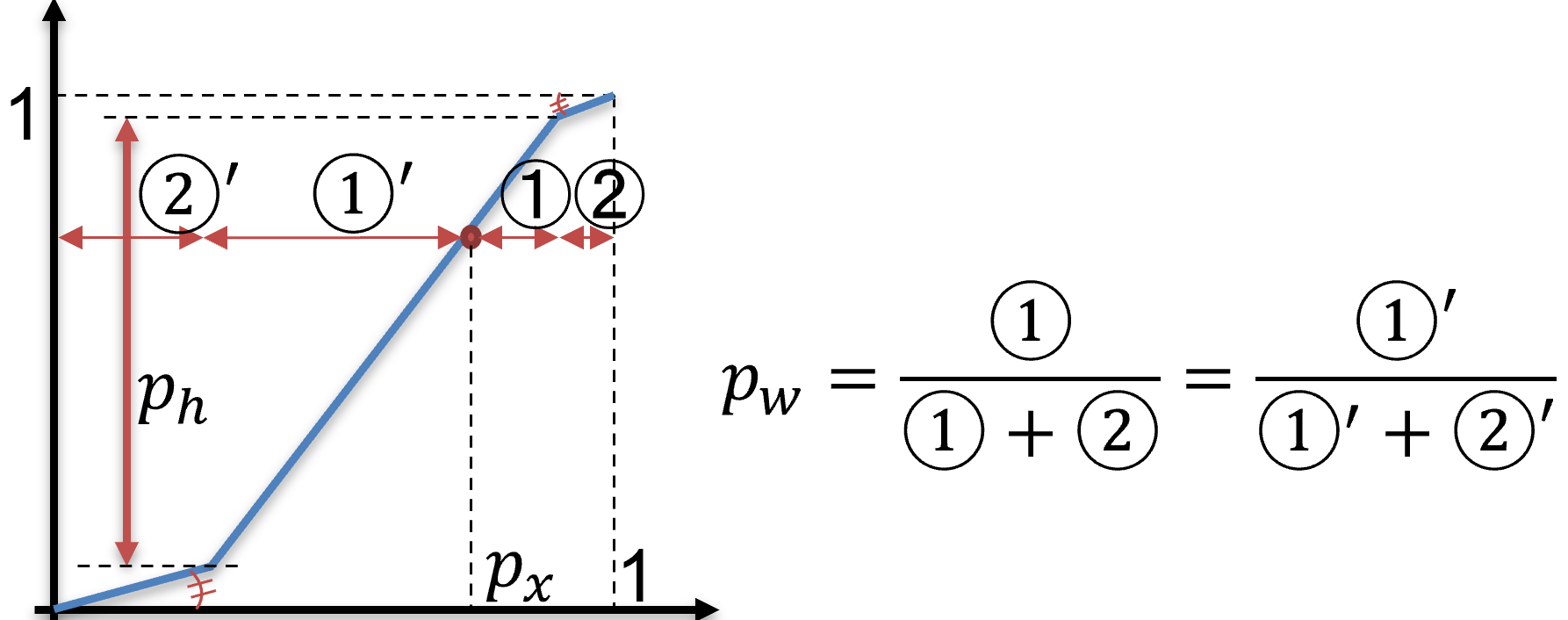
Figure 5: Auto gain function without clipping.

Denoiser (DN)

We utilize a simple Bilateral filter (BF) [41] as,

$$I_{DN}\left(X\right)=\left(1-p_{a}\right)\cdot X+p_{a}\cdot BF\left(p_{\sigma s},p_{\sigma i};X\right),$$ (7)

where $p_{\sigma s}$ and $p_{\sigma i}$ are the parameters for the spatial and intensity variance and $p_{a}$ is another parameter. We set the kernel size as five.

Sharpener (SN)

Simple Gaussian filter (GF) is used as,

$$I_{SN}\left(X\right)=\left(1-p_{a}\right)\cdot X+p_{a}\cdot\left(X-GF\left(p_{\sigma};X\right)\right).$$ (8)

The second term is the difference-of-Gaussians [26] whose kernel sizes are one and five;

$$DoG(X) =GF(p_{\sigma 1},k_{1};X)-GF(p_{\sigma},k_{2};X)$$

$$=X-GF(p_{\sigma},5;X).$$ (9)

Gamma (GM)

We follow the parameterization of gamma tone mapping in [29, 48] and implement it as differentiable;

$$I_{GM}\left(X\right)=X^{\frac{1}{p_{\text{1}}}\cdot\frac{1-\left(1-p_{\text{2}}\right)X^{\frac{1}{p_{\text{1}}}}}{1-\left(1-p_{\text{2}}\right)p_{k}^{\frac{1}{\text{$p_{\text{1}}$}}}}}.$$ (10)

Contrast Stretcher (CS)

We implement CS as a simple linear function of $I_{CS}\left(X\right)=q_{b}X+q_{c}$. Because DNN can process any range of value, we do not restrict the range.

Appendix B Additional Evaluations

B.1 Evaluation on Human Detection

Multi-Layer Control

A more detailed ablation study is performed for multi-layer control. Here, we add ISP layers in order of effect one by one. As the Table 8 shows, the proposed method without LU struggles to control multi-layer ISPs. The proposed LU successfully disentangles the difficulty of multi-layer control and boosts the accuracy from the setting of only containing GM tone mapping.

Table 8: Control of Multi-layer ISPs on the human detection dataset. We add ISP layers in order of effect.

ISP components	w/o LU	w/ LU
GM	48.9	-
GM+CS	49.4	49.4
DN+GM+CS	49.2	49.4
DN+SN+GM+CS	48.0	49.5

Comparison with Other Possible Controllers

(a) Feedforward control from a single-feature.	(b) Feedforward control from multi-features.
(c) Feedforward control by exemplifications
when using several ISP parameter sets [8].	(d) Feedback control from a single-feature (ours).

Figure 6: Comparison with other possible controllers. The (a) is the most lightweight possible controller among feedforward control. The (b) is based on typical dynamic neural network architectures [47, 6, 7]. The (c) is a more advanced method of the (b) proposed for RAW image reconstruction [8]. The (d) is the proposed efficient feedback control.

Table 9: Comparison with other possible controllers on the human detection dataset. $C$ is the computational cost of the ISP. ResNet18 or 4-layer CNN is used as the encoder for feedforward controls.

ISP		GFLOPS	#params [M]	latency [ms]	controller [ms]	AP [%]
GM	(a) (encoder = 4-layer CNN)	14.03+C	14.33	11.2	3.3	47.5
	+ our ``RO+''	14.03+C	14.33	11.5	3.6	48.8
	(a) (encoder = ResNet18)	20.99+C	25.77	13.2	5.3	46.1
	+ our ``RO+''	20.99+C	25.77	13.6	5.7	49.4
	(d) ours	13.65+C	15.66	8.3	0.4	49.1
DN+SN+GM+CS	(a) (encoder = ResNet18)	20.99+C	25.77	31.1$\spadesuit$	5.3	48.3
	+ our ``RO+'' and ``LU''	20.99+C	25.87	31.6$\spadesuit$	5.8	48.5
	(b) (encoder = 4-layer CNN)	15.23+C	14.72	29.1$\spadesuit$	3.3	47.7
	+ our ``RO+''	15.23+C	14.72	29.5$\spadesuit$	3.7	49.0
	(c) (encoder = 4-layer CNN)	15.93+6C	14.73	101.1$\spadesuit$	9.2 $\clubsuit$	49.4
	(d) ours	13.65+C	15.76	27.7$\spadesuit$	1.9	49.6

$\spadesuit$: Our implementations of DN and SN have a lot of duplicate calculations and are not optimized.

$\clubsuit$: Because of the above, the controller's latency is measured in case all four layers are GM to make a fair comparison.

Table 10: Detailed evaluation on LODDataset [15] trained with simulated RAW-like data converted from COCO Dataset [19].

	mAP@0.5:0.95 per exposure ratio to default
	1/10	1/20	1/30	1/40	1/50	1/100	Ave.
as is	23.3	16.7	14.4	114.1	13.4	3.6	14.3
SID [4]	25.8	20.0	16.4	15.1	13.2	6.7	16.2
Zero DCE [10]	32.5	25.3	23.4	21.5	17.8	8.9	21.6
REDI [18]	33.6	30.2	26.1	24.6	23.4	14.1	25.4
H. Yang et. al. [15]	38.5	31.7	29.3	27.8	27.1	18.1	28.8
diff. tuning (GM) [48]	42.8	34.9	39.5	38.9	29.4	12.6	33.0
NeuralAE (GM)[32]	42.3	35.3	38.5	40.6	29.9	15.6	33.7
NeuralAE (GM+CS)[32]	37.0	31.5	33.4	35.1	28.5	18.3	30.6
ours (GM)	45.2	41.1	51.1	49.1	41.4	33.9	43.6
ours (AG+GM+CS)	45.8	41.1	52.1	48.6	41.2	34.9	44.0

In this section, the proposed controller is compared with other possible controllers, especially feedforward controllers because most of the dynamic neural networks methods [47, 6, 7] have successfully controlled DNN parameters based on feedforward controls. Fig. 6(a) controls all functions based on a single-feature. It is different from the typical controllers for dynamic neural networks [47, 6, 7] but the most lightweight possible feedforward controller. Fig. 6(b) is based on typical dynamic neural network architectures that control each layer with an output of the previous layer. The problem in applying it to the ISP control is that the output of the previous layer is just an image, so it is necessary to create features from scratch using an encoder. Fig. 6(c) is a more advanced method of Fig. 6(b) proposed for RAW image reconstruction [8]. Several processed images with different parameter sets are input to the encoder as exemplifications, and the output parameters from the encoder are determined as the weighted average of the parameter sets. Note that the inverse pipeline is not implemented because it is trained only with detection loss in our problem setup. The number of exemplifications is set as five. We use two types of networks with different computational costs as encoders in Fig. 6(a), (b), and (c): ResNet18 [13] or 4-layer light-weight CNNs with ReLU activations, whose kernel sizes, strides, and output channel sizes are (3, 3, 3, 3), (2, 2, 2, 2), and (16, 32, 64, 128). Fig. 6(d) is the proposed feedback control from a feature.

The results are shown in Table 9. In the case of the single-layer ISP setting, the feedforward control exceeds the accuracy of the proposed method by using a large encoder (ResNet18). However, in the experimental setting with the 4-layer CNN, where the computational cost is still higher than the proposed method, the accuracy is inferior. This result indicates that the feedback control is more efficient. By adding more convolutions to the ``Semantic Feature Branch'' (SFB), the proposed feedback control might improve the accuracy. In our setting, SFB contains only one convolution layer. In addition, the proposed RO+ for controlling a difficult function is found to be effective even for the feedforward controls.

In the case of the multi-layer ISP setting, the proposed method outperforms feedforward controls with lower computational cost. Although the (c) architecture is accurate, it takes a high computational cost because it needs multiple computations of ISPs and encoders. Limitted to feedforward controls, a comparison of (a) and (b) shows that it is more efficient to encode the previous layer's image with multiple small encoders than with one large encoder. On the other hand, our feedback control achieves higher accuracy despite the fact that the control is based on a single shallow layer of feature (the output of the first stage of the detector's ResNet18 backbone). This should be because the following two factors outweigh the difficulty of controlling from a single encoder. One factor should be the advantage that the controller is able to extract what is captured by the detector directly. The other factor should be the effectiveness of the proposed training method for feedback control (PI).

Lastly, the proposed method is lightweight because it does not require image encoders and performs almost only 1D tensor operations.

B.2 Evaluation on Low-Light Recognition

Training with Simulated RAW Images

A more detailed comparison than Table 7 of the main paper is shown in Table 10. It is broken down by the level of under-exposure. Our method obtains the highest accuracy among all levels of under-exposure. The dynamic ISP control is able to convert a broad luminance distribution environment to a preferable distribution for the detector. The visualized comparison is in Fig. 7 and Fig. 8.

Training with Real Dark RAW Images

We also evaluate the case of real RAW images used for training. The real RAW images are randomly split into training data of 1830 images and test data of 400, the same with [15]. The result is shown in Table 11. Our method is confirmed effective for small amounts of real RAW training data.

Table 11: Evaluation on LODDataset [15] trained with real dark RAW data in LODDataset.

	ISP	mAP@0.5:0.95
H. Yang et. al. [15]	-	44.7
NeuralAE [32]	GM	45.0
NeuralAE [32]	GM+CS	45.5
ours	GM	45.4
ours	AG+GM+CS	46.2

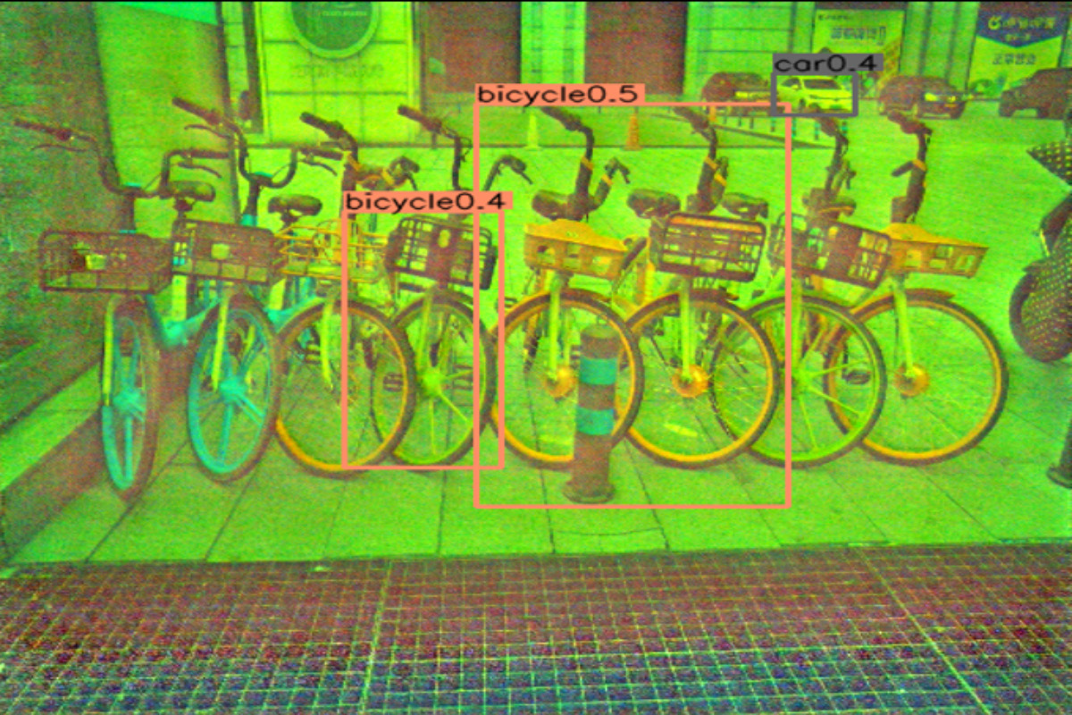
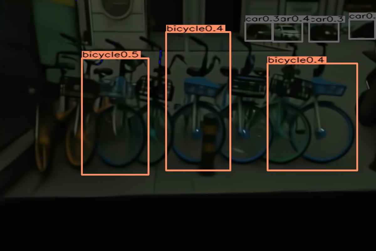
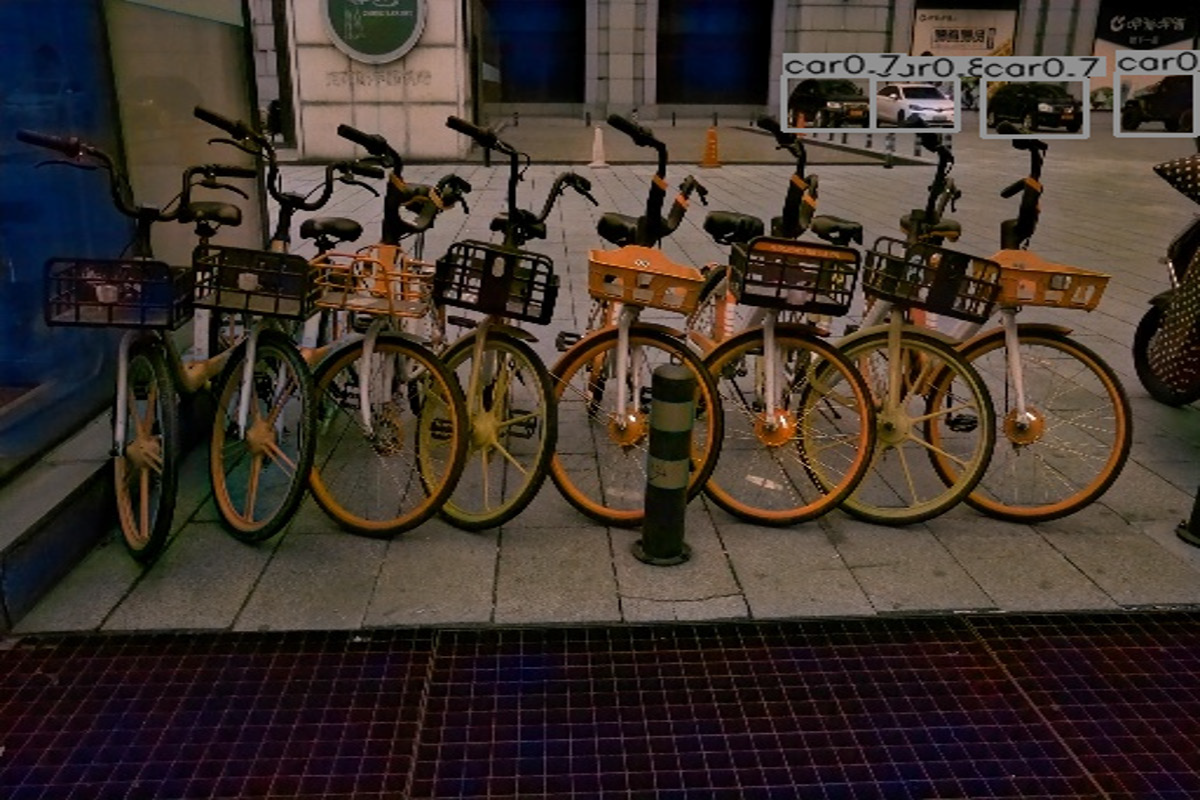
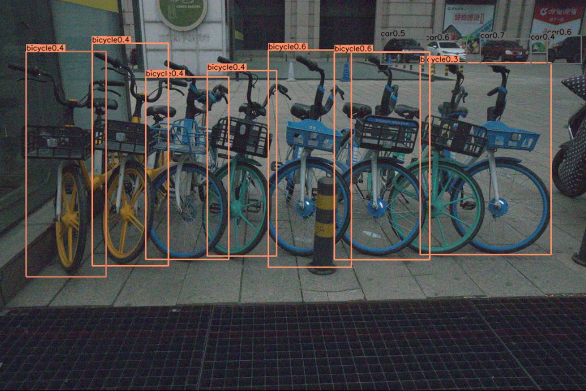
SID [4]	Zero DCE [10]	REDI [18]	H. Yang et. al. [15]
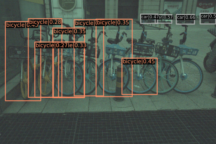
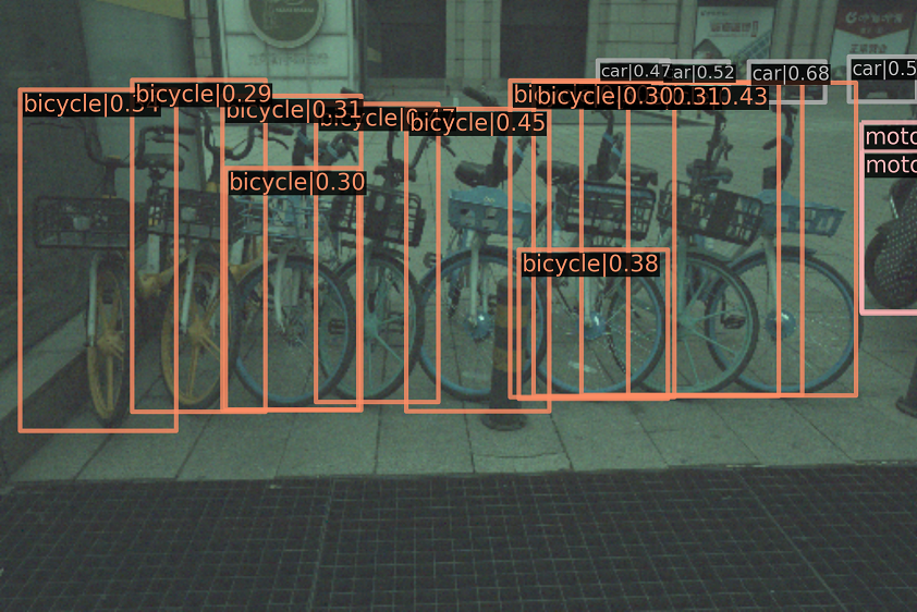
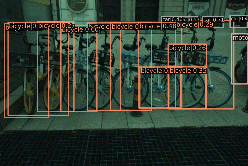
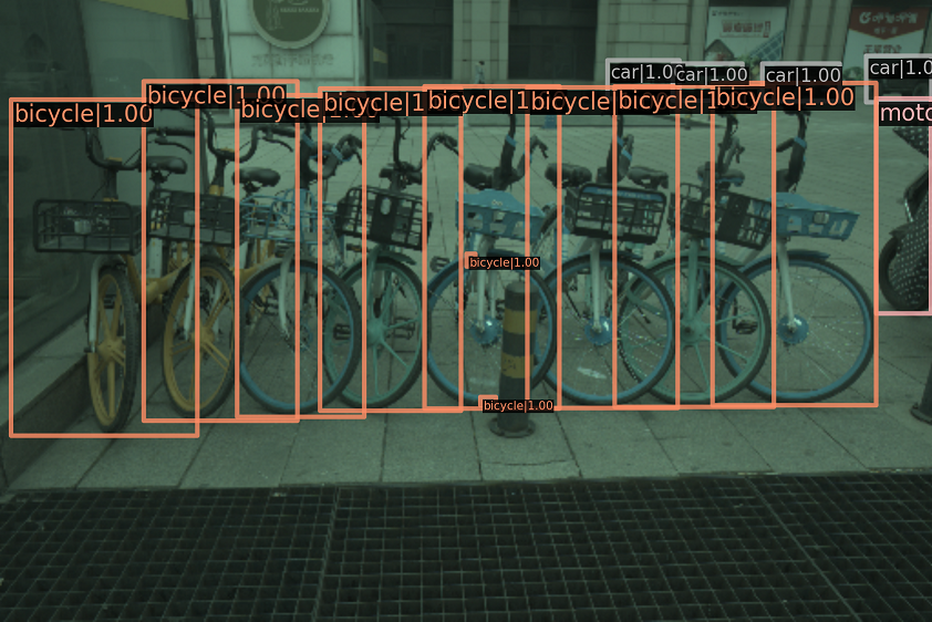
diff. tuning (GM) [48]	NeuralAE (GM)[32]	ours (AG+GM+CS)	GT
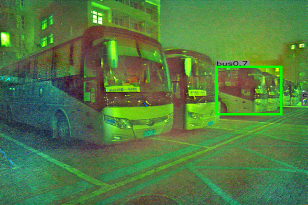
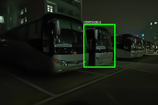
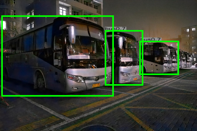
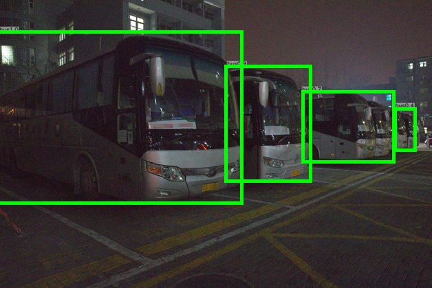
SID [4]	Zero DCE [10]	REDI [18]	H. Yang et. al. [15]
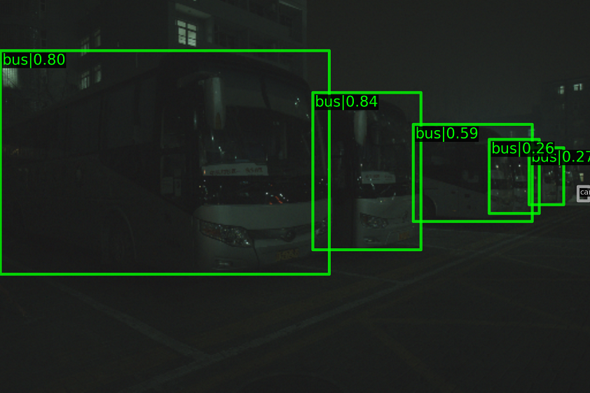
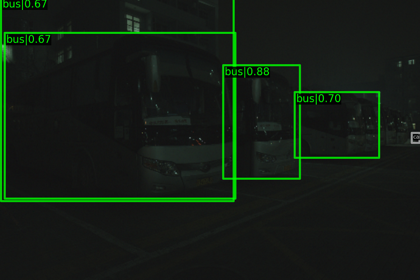
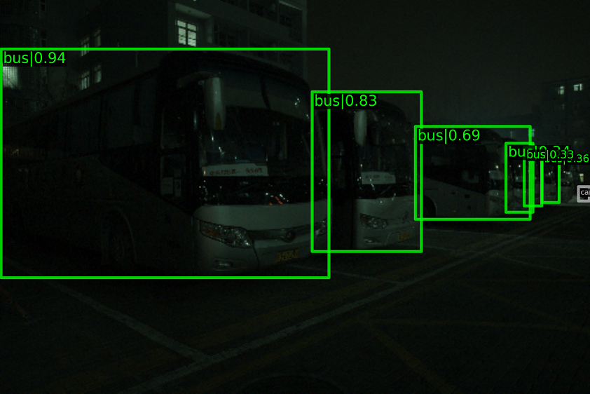
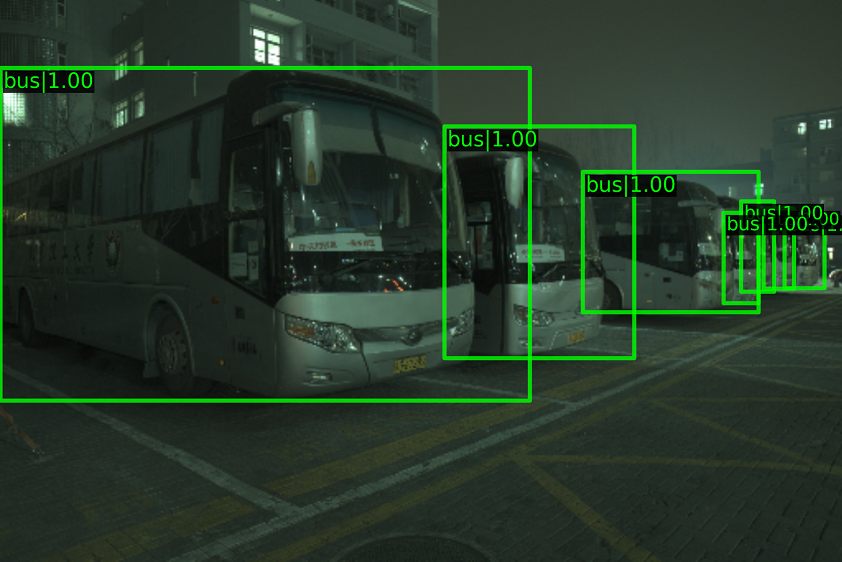
diff. tuning (GM) [48]	NeuralAE (GM)[32]	ours (AG+GM+CS)	GT
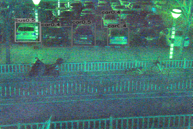
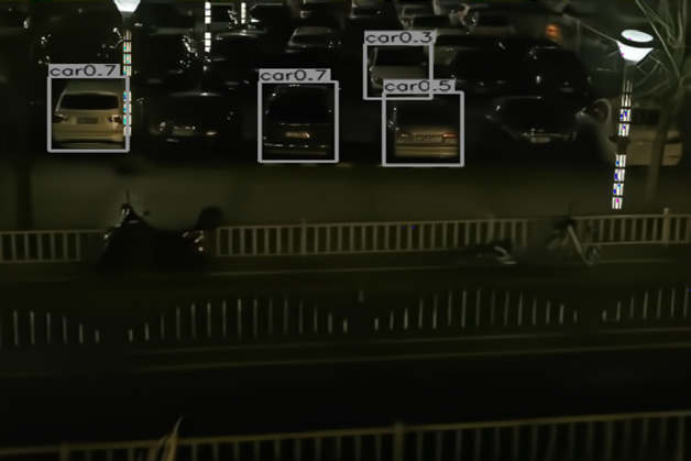
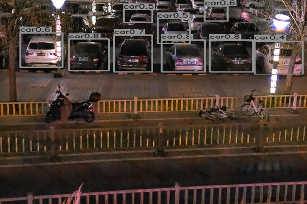
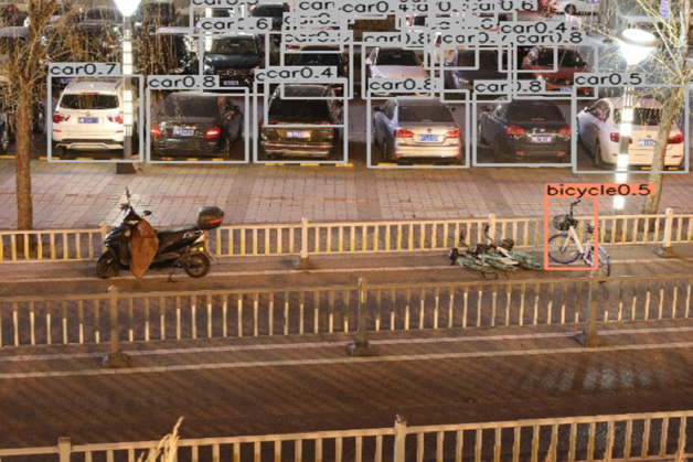
SID [4]	Zero DCE [10]	REDI [18]	H. Yang et. al. [15]
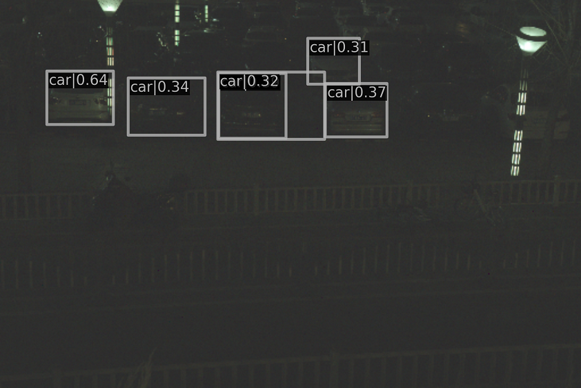
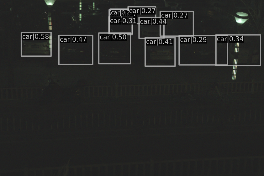
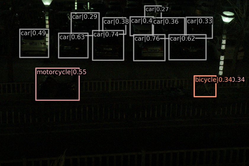
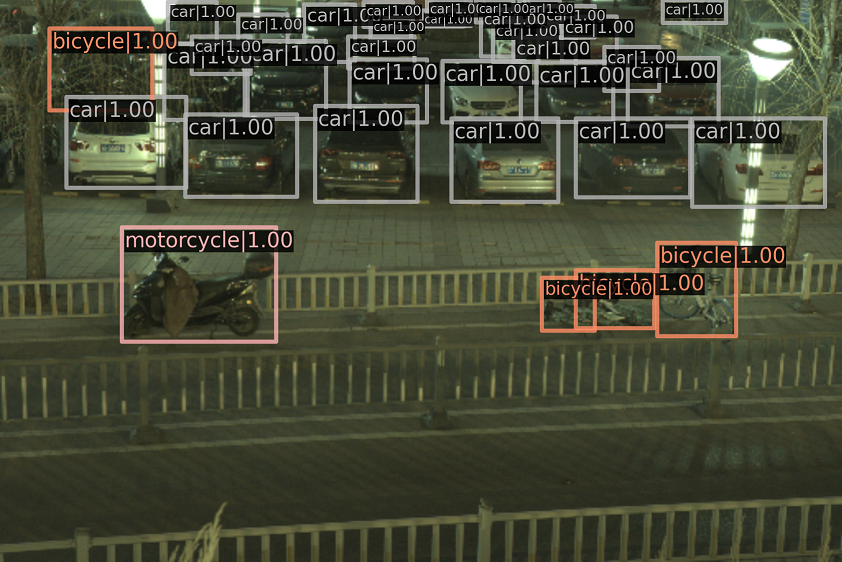
diff. tuning (GM) [48]	NeuralAE (GM)[32]	ours (AG+GM+CS)	GT

Figure 7: The visualization result on LODDataset [15] trained with simulated RAW-like data converted from COCO Dataset [19]. The results of SID, Zero DCE, REDI, and H. Yang et. al. are from the [15]'s paper.

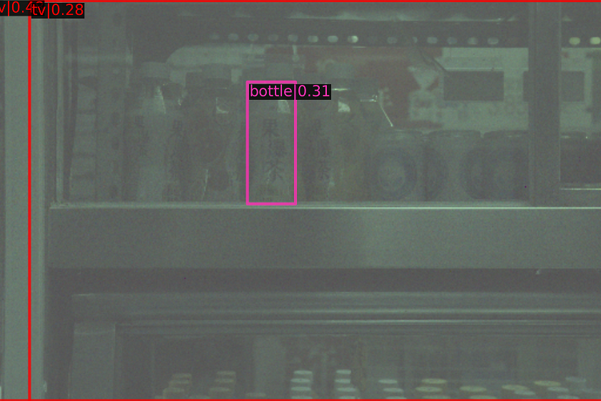
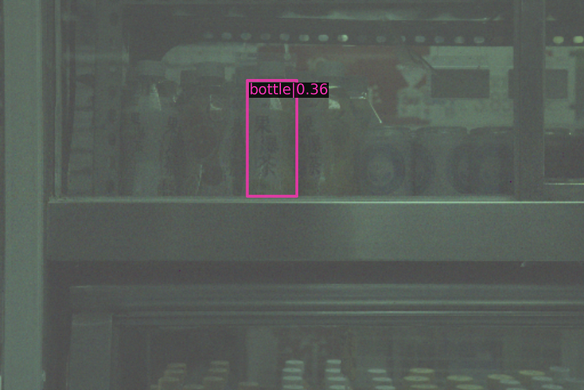
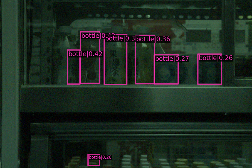
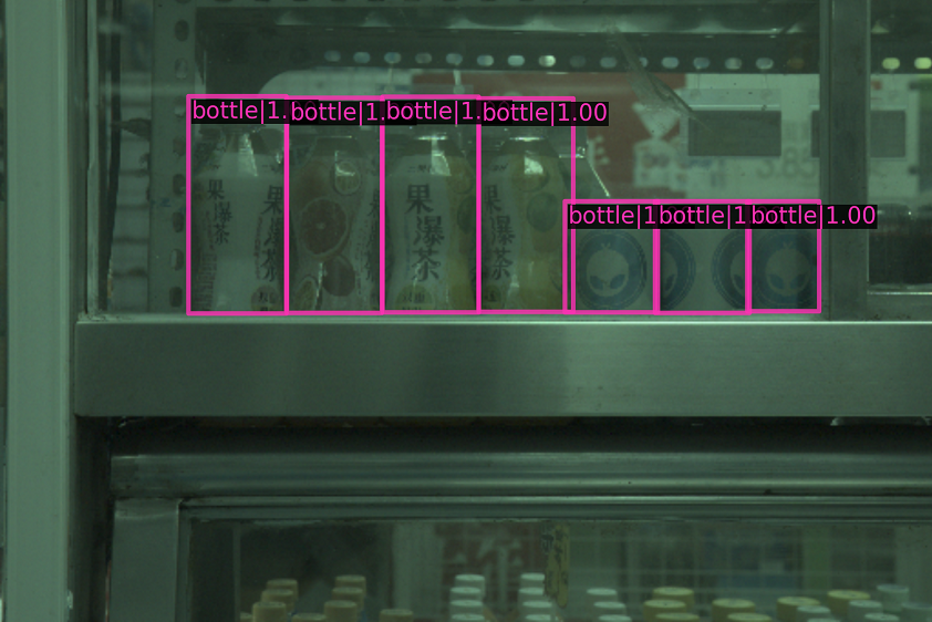
diff. tuning (GM) [48]	NeuralAE (GM)[32]	ours (AG+GM+CS)	GT
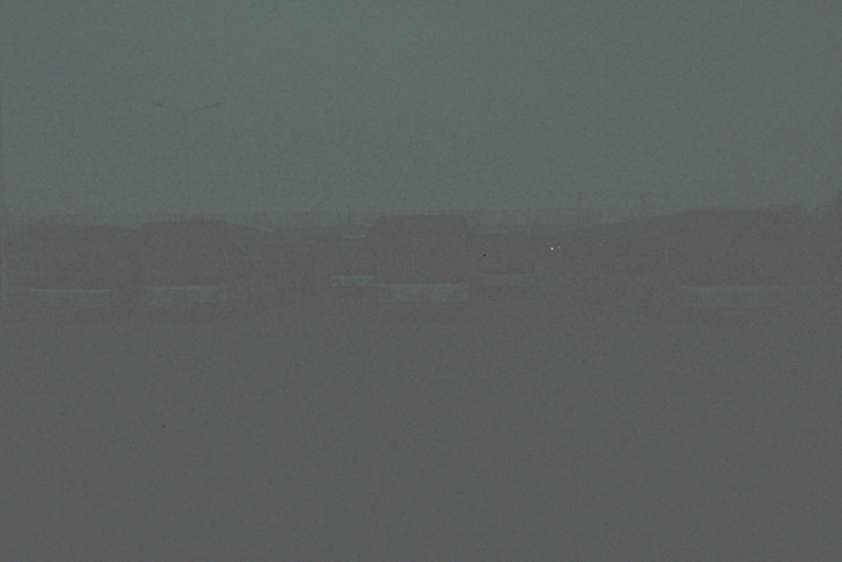
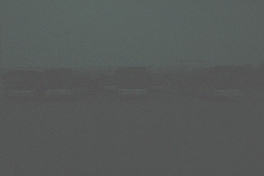
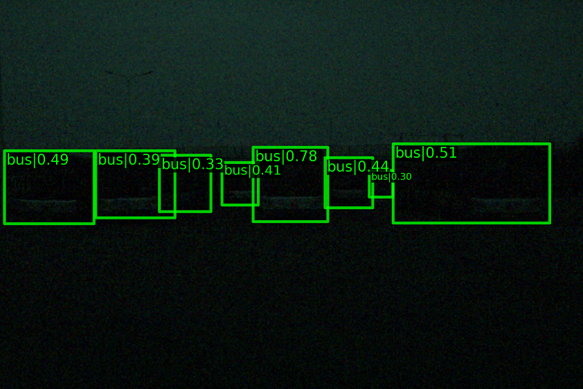
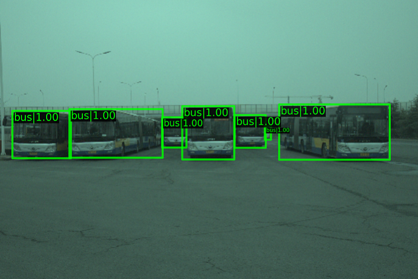
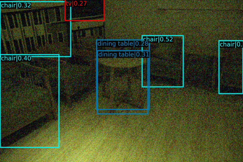
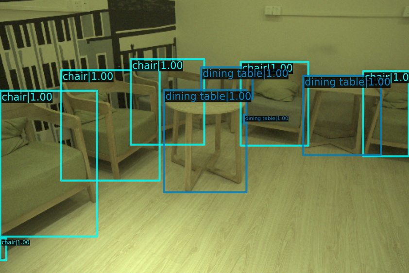
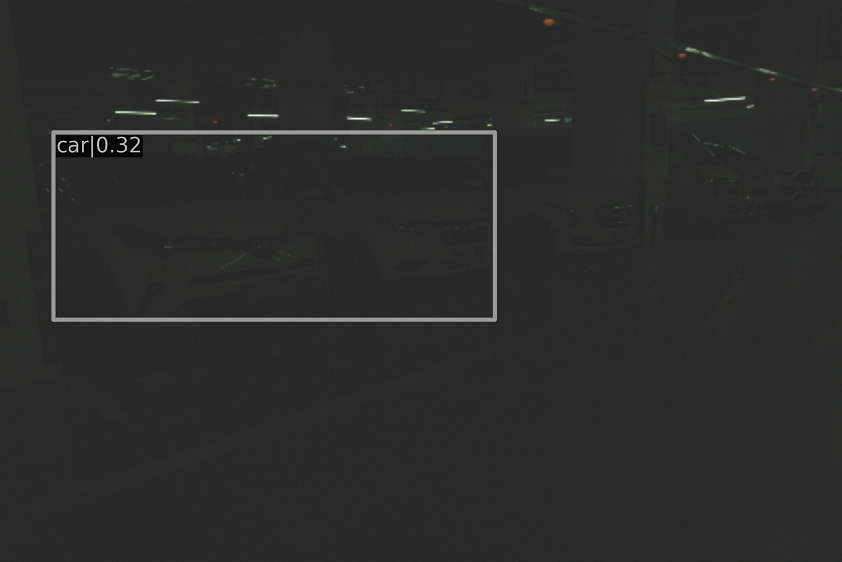
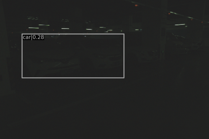
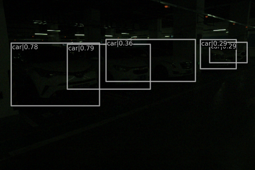
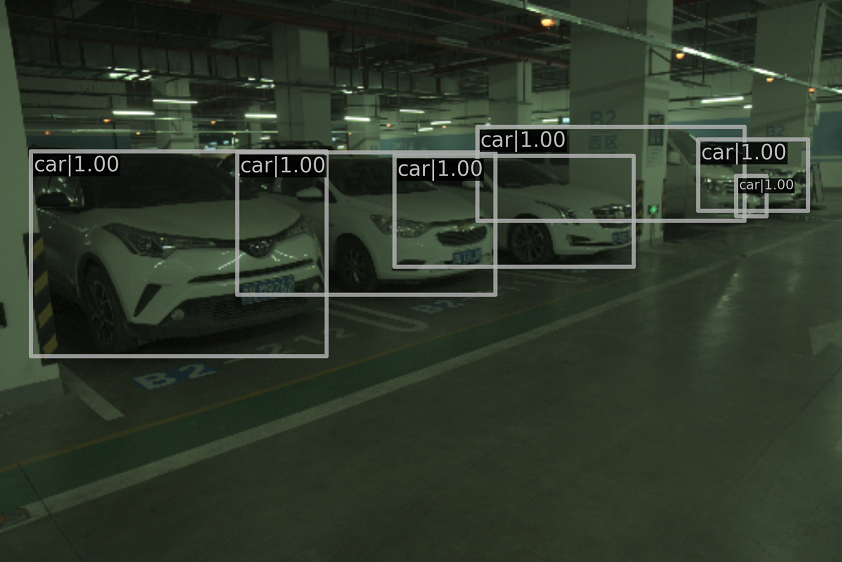
diff. tuning (GM) [48]	NeuralAE (GM)[32]	ours (AG+GM+CS)	GT
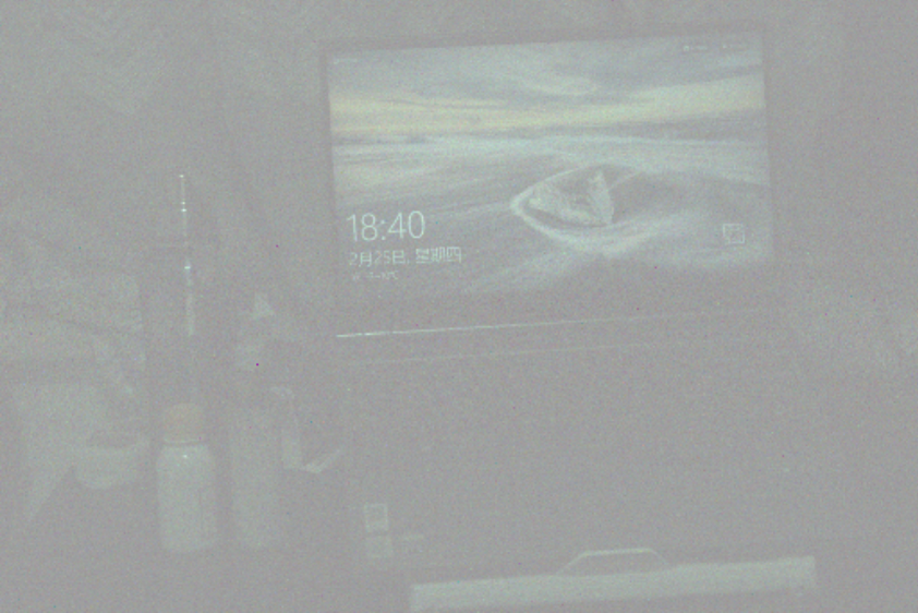
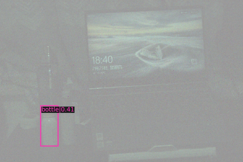
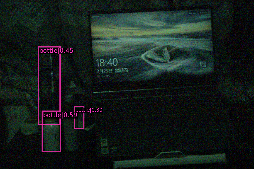
diff. tuning (GM) [48]	NeuralAE (GM)[32]	ours (AG+GM+CS)	GT
diff. tuning (GM) [48]	NeuralAE (GM)[32]	ours (AG+GM+CS)	GT
diff. tuning (GM) [48]	NeuralAE (GM)[32]	ours (AG+GM+CS)	GT

Figure 8: The visualization result on LODDataset [15] trained with simulated RAW-like data converted from COCO Dataset [19]. More challenging images than images in Fig. 7 are collected.

References

- [1] Mahmoud Afifi, Jonathan T Barron, Chloe LeGendre, Yun-Ta Tsai, and Francois Bleibel. Cross-camera convolutional color constancy. In Proceedings of the IEEE/CVF International Conference on Computer Vision, pages 1981–1990, 2021.
- [2] Tim Brooks, Ben Mildenhall, Tianfan Xue, Jiawen Chen, Dillon Sharlet, and Jonathan T Barron. Unprocessing images for learned raw denoising. In Proceedings of the IEEE/CVF Conference on Computer Vision and Pattern Recognition, pages 11036–11045, 2019.
- [3] Mark Buckler, Suren Jayasuriya, and Adrian Sampson. Reconfiguring the imaging pipeline for computer vision. In Proceedings of the IEEE International Conference on Computer Vision, pages 975–984, 2017.
- [4] Chen Chen, Qifeng Chen, Jia Xu, and Vladlen Koltun. Learning to see in the dark. In Proceedings of the IEEE conference on computer vision and pattern recognition, pages 3291–3300, 2018.
- [5] Liangyu Chen, Xin Lu, Jie Zhang, Xiaojie Chu, and Chengpeng Chen. Hinet: Half instance normalization network for image restoration. In Proceedings of the IEEE/CVF Conference on Computer Vision and Pattern Recognition, pages 182–192, 2021.
- [6] Yinpeng Chen, Xiyang Dai, Mengchen Liu, Dongdong Chen, Lu Yuan, and Zicheng Liu. Dynamic convolution: Attention over convolution kernels. In Proceedings of the IEEE/CVF Conference on Computer Vision and Pattern Recognition, pages 11030–11039, 2020.
- [7] Yinpeng Chen, Xiyang Dai, Mengchen Liu, Dongdong Chen, Lu Yuan, and Zicheng Liu. Dynamic relu. In European Conference on Computer Vision, pages 351–367. Springer, 2020.
- [8] Marcos V Conde, Steven McDonagh, Matteo Maggioni, Ales Leonardis, and Eduardo Pérez-Pellitero. Model-based image signal processors via learnable dictionaries. In Proceedings of the AAAI Conference on Artificial Intelligence, volume 36, pages 481–489, 2022.
- [9] Steven Diamond, Vincent Sitzmann, Frank Julca-Aguilar, Stephen Boyd, Gordon Wetzstein, and Felix Heide. Dirty pixels: Towards end-to-end image processing and perception. ACM Transactions on Graphics (TOG), 40(3):1–15, 2021.
- [10] Chunle Guo, Chongyi Li, Jichang Guo, Chen Change Loy, Junhui Hou, Sam Kwong, and Runmin Cong. Zero-reference deep curve estimation for low-light image enhancement. In Proceedings of the IEEE/CVF Conference on Computer Vision and Pattern Recognition, pages 1780–1789, 2020.
- [11] Patrick Hansen, Alexey Vilkin, Yury Krustalev, James Imber, Dumidu Talagala, David Hanwell, Matthew Mattina, and Paul N Whatmough. Isp4ml: The role of image signal processing in efficient deep learning vision systems. In 2020 25th International Conference on Pattern Recognition (ICPR), pages 2438–2445. IEEE, 2021.
- [12] Kaiming He, Xiangyu Zhang, Shaoqing Ren, and Jian Sun. Delving deep into rectifiers: Surpassing human-level performance on imagenet classification. In Proceedings of the IEEE international conference on computer vision, pages 1026–1034, 2015.
- [13] Kaiming He, Xiangyu Zhang, Shaoqing Ren, and Jian Sun. Deep residual learning for image recognition. In Proceedings of the IEEE conference on computer vision and pattern recognition, pages 770–778, 2016.
- [14] Luis V Hevia, Miguel A Patricio, Joseé M Molina, and Antonio Berlanga. Optimization of the isp parameters of a camera through differential evolution. IEEE Access, 8:143479–143493, 2020.
- [15] Yang Hong, Kaixuan Wei, Linwei Chen, and Ying Fu. Crafting object detection in very low light. In Proceedings of the British Machine Vision Virtual Conference, 2021.
- [16] Yifan Jiang, Xinyu Gong, Ding Liu, Yu Cheng, Chen Fang, Xiaohui Shen, Jianchao Yang, Pan Zhou, and Zhangyang Wang. Enlightengan: Deep light enhancement without paired supervision. IEEE Transactions on Image Processing, 30:2340–2349, 2021.
- [17] Diederik P Kingma and Jimmy Ba. Adam: A method for stochastic optimization. arXiv preprint arXiv:1412.6980, 2014.
- [18] Mohit Lamba and Kaushik Mitra. Restoring extremely dark images in real time. In Proceedings of the IEEE/CVF Conference on Computer Vision and Pattern Recognition, pages 3487–3497, 2021.
- [19] Tsung-Yi Lin, Michael Maire, Serge Belongie, James Hays, Pietro Perona, Deva Ramanan, Piotr Dollár, and C Lawrence Zitnick. Microsoft coco: Common objects in context. In European conference on computer vision, pages 740–755. Springer, 2014.
- [20] Hanxiao Liu, Karen Simonyan, and Yiming Yang. Darts: Differentiable architecture search. arXiv preprint arXiv:1806.09055, 2018.
- [21] Shuai Liu, Chaoyu Feng, Xiaotao Wang, Hao Wang, Ran Zhu, Yongqiang Li, and Lei Lei. Deep-flexisp: A three-stage framework for night photography rendering. In Proceedings of the IEEE/CVF Conference on Computer Vision and Pattern Recognition, pages 1211–1220, 2022.
- [22] Zili Liu, Tu Zheng, Guodong Xu, Zheng Yang, Haifeng Liu, and Deng Cai. Training-time-friendly network for real-time object detection. In proceedings of the AAAI conference on artificial intelligence, volume 34, pages 11685–11692, 2020.
- [23] Ilya Loshchilov and Frank Hutter. Sgdr: Stochastic gradient descent with warm restarts. arXiv preprint arXiv:1608.03983, 2016.
- [24] Feifan Lv, Feng Lu, Jianhua Wu, and Chongsoon Lim. Mbllen: Low-light image/video enhancement using cnns. In BMVC, volume 220, page 4, 2018.
- [25] Long Ma, Tengyu Ma, Risheng Liu, Xin Fan, and Zhongxuan Luo. Toward fast, flexible, and robust low-light image enhancement. In Proceedings of the IEEE/CVF Conference on Computer Vision and Pattern Recognition, pages 5637–5646, 2022.
- [26] David Marr and Ellen Hildreth. Theory of edge detection. Proceedings of the Royal Society of London. Series B. Biological Sciences, 207(1167):187–217, 1980.
- [27] Kristina Monakhova, Stephan R Richter, Laura Waller, and Vladlen Koltun. Dancing under the stars: video denoising in starlight. In Proceedings of the IEEE/CVF Conference on Computer Vision and Pattern Recognition, pages 16241–16251, 2022.
- [28] Igor Morawski, Yu-An Chen, Yu-Sheng Lin, Shusil Dangi, Kai He, and Winston H Hsu. Genisp: Neural isp for low-light machine cognition. In Proceedings of the IEEE/CVF Conference on Computer Vision and Pattern Recognition, pages 630–639, 2022.
- [29] Ali Mosleh, Avinash Sharma, Emmanuel Onzon, Fahim Mannan, Nicolas Robidoux, and Felix Heide. Hardware-in-the-loop end-to-end optimization of camera image processing pipelines. In Proceedings of the IEEE/CVF Conference on Computer Vision and Pattern Recognition, pages 7529–7538, 2020.
- [30] Jun Nishimura, Timo Gerasimow, Rao Sushma, Aleksandar Sutic, Chyuan-Tyng Wu, and Gilad Michael. Automatic isp image quality tuning using nonlinear optimization. In 2018 25th IEEE International Conference on Image Processing (ICIP), pages 2471–2475. IEEE, 2018.
- [31] Taishi Ono, Yuhi Kondo, Legong Sun, Teppei Kurita, and Yusuke Moriuchi. Degree-of-linear-polarization-based color constancy. In Proceedings of the IEEE/CVF Conference on Computer Vision and Pattern Recognition, pages 19740–19749, 2022.
- [32] Emmanuel Onzon, Fahim Mannan, and Felix Heide. Neural auto-exposure for high-dynamic range object detection. In Proceedings of the IEEE/CVF Conference on Computer Vision and Pattern Recognition, pages 7710–7720, 2021.
- [33] Adam Paszke, Sam Gross, Francisco Massa, Adam Lerer, James Bradbury, Gregory Chanan, Trevor Killeen, Zeming Lin, Natalia Gimelshein, Luca Antiga, et al. Pytorch: An imperative style, high-performance deep learning library. Advances in neural information processing systems, 32, 2019.
- [34] G Pavithra and Bhat Radhesh. Automatic image quality tuning framework for optimization of isp parameters based on multi-stage optimization approach. Electronic Imaging, 2021(9):197–1, 2021.
- [35] Abhijith Punnappurath, Abdullah Abuolaim, Abdelrahman Abdelhamed, Alex Levinshtein, and Michael S Brown. Day-to-night image synthesis for training nighttime neural isps. In Proceedings of the IEEE/CVF Conference on Computer Vision and Pattern Recognition, pages 10769–10778, 2022.
- [36] Erik Reinhard, Wolfgang Heidrich, Paul Debevec, Sumanta Pattanaik, Greg Ward, and Karol Myszkowski. High dynamic range imaging: acquisition, display, and image-based lighting. Morgan Kaufmann, 2010.
- [37] Nicolas Robidoux, Luis E Garcia Capel, Dong-eun Seo, Avinash Sharma, Federico Ariza, and Felix Heide. End-to-end high dynamic range camera pipeline optimization. In Proceedings of the IEEE/CVF Conference on Computer Vision and Pattern Recognition, pages 6297–6307, 2021.
- [38] Olaf Ronneberger, Philipp Fischer, and Thomas Brox. U-net: Convolutional networks for biomedical image segmentation. In Medical Image Computing and Computer-Assisted Intervention–MICCAI 2015: 18th International Conference, Munich, Germany, October 5-9, 2015, Proceedings, Part III 18, pages 234–241. Springer, 2015.
- [39] Eli Schwartz, Alex Bronstein, and Raja Giryes. Isp distillation. arXiv preprint arXiv:2101.10203, 2021.
- [40] Stanley S Stevens. On the psychophysical law. Psychological review, 64(3):153–181, 1957.
- [41] Carlo Tomasi and Roberto Manduchi. Bilateral filtering for gray and color images. In Sixth international conference on computer vision (IEEE Cat. No. 98CH36271), pages 839–846. IEEE, 1998.
- [42] Ethan Tseng, Felix Yu, Yuting Yang, Fahim Mannan, Karl ST Arnaud, Derek Nowrouzezahrai, Jean-François Lalonde, and Felix Heide. Hyperparameter optimization in black-box image processing using differentiable proxies. ACM Trans. Graph., 38(4):27–1, 2019.
- [43] Zhengzhong Tu, Hossein Talebi, Han Zhang, Feng Yang, Peyman Milanfar, Alan Bovik, and Yinxiao Li. Maxim: Multi-axis mlp for image processing. In Proceedings of the IEEE/CVF Conference on Computer Vision and Pattern Recognition, pages 5769–5780, 2022.
- [44] Chen Wei, Wenjing Wang, Wenhan Yang, and Jiaying Liu. Deep retinex decomposition for low-light enhancement. arXiv preprint arXiv:1808.04560, 2018.
- [45] Jay Whang, Mauricio Delbracio, Hossein Talebi, Chitwan Saharia, Alexandros G Dimakis, and Peyman Milanfar. Deblurring via stochastic refinement. In Proceedings of the IEEE/CVF Conference on Computer Vision and Pattern Recognition, pages 16293–16303, 2022.
- [46] Chyuan-Tyng Wu, Leo F Isikdogan, Sushma Rao, Bhavin Nayak, Timo Gerasimow, Aleksandar Sutic, Liron Ain-kedem, and Gilad Michael. Visionisp: Repurposing the image signal processor for computer vision applications. In 2019 IEEE International Conference on Image Processing (ICIP), pages 4624–4628. IEEE, 2019.
- [47] Brandon Yang, Gabriel Bender, Quoc V Le, and Jiquan Ngiam. Condconv: Conditionally parameterized convolutions for efficient inference. Advances in Neural Information Processing Systems, 32, 2019.
- [48] Masakazu Yoshimura, Junji Otsuka, Atsushi Irie, and Takeshi Ohashi. Rawgment: Noise-accounted raw augmentation enables recognition in a wide variety of environments. arXiv preprint arXiv:2210.16046, 2022.
- [49] Ke Yu, Zexian Li, Yue Peng, Chen Change Loy, and Jinwei Gu. Reconfigisp: Reconfigurable camera image processing pipeline. In Proceedings of the IEEE/CVF International Conference on Computer Vision, pages 4248–4257, 2021.
- [50] Meina Zhang, Yingying Fang, Guoxi Ni, and Tieyong Zeng. Pixel screening based intermediate correction for blind deblurring. In Proceedings of the IEEE/CVF Conference on Computer Vision and Pattern Recognition, pages 5892–5900, 2022.
- [51] Yi Zhang, Dasong Li, Ka Lung Law, Xiaogang Wang, Hongwei Qin, and Hongsheng Li. Idr: Self-supervised image denoising via iterative data refinement. In Proceedings of the IEEE/CVF Conference on Computer Vision and Pattern Recognition, pages 2098–2107, 2022.
- [52] Yonghua Zhang, Jiawan Zhang, and Xiaojie Guo. Kindling the darkness: A practical low-light image enhancer. In Proceedings of the 27th ACM international conference on multimedia, pages 1632–1640, 2019.
- [53] Xingyi Zhou, Dequan Wang, and Philipp Krähenbühl. Objects as points. arXiv preprint arXiv:1904.07850, 2019.