Nonparametric Involutive Markov Chain Monte Carlo

Nonparametric Hamiltonian Monte Carlo (Appendix)

Abstract

A challenging problem in probabilistic programming is to develop inference algorithms that work for arbitrary programs in a universal probabilistic programming language (PPL). We present the nonparametric involutive Markov chain Monte Carlo (NP-iMCMC) algorithm as a method for constructing MCMC inference algorithms for nonparametric models expressible in universal PPLs. Building on the unifying involutive MCMC framework, and by providing a general procedure for driving state movement between dimensions, we show that NP-iMCMC can generalise numerous existing iMCMC algorithms to work on nonparametric models. We prove the correctness of the NP-iMCMC sampler. Our empirical study shows that the existing strengths of several iMCMC algorithms carry over to their nonparametric extensions. Applying our method to the recently proposed Nonparametric HMC, an instance of (Multiple Step) NP-iMCMC, we have constructed several nonparametric extensions (all of which new) that exhibit significant performance improvements.

1 Introduction

Universal probabilistic programming (Goodman et al., 2008) is the idea of writing probabilistic models in a Turing-complete programming language. A universal probabilistic programming language (PPL) can express all computable probabilistic models (Vákár et al., 2019), using only a handful of basic programming constructs such as branching and recursion. In particular, nonparametric models, where the number of random variables is not determined a priori and possibly unbounded, can be described naturally in a universal PPL. In programming language terms, this means the number of sample statements is unknown prior to execution. On the one hand, such programs can describe probabilistic models with an unknown number of components, such as Bayesian nonparametric models (Richardson & Green, 1997), variable selection in regression (Ratner, 2010), and models for signal processing (Murray et al., 2018). On the other hand, there are models defined on infinite-dimensional spaces, such as probabilistic context free grammars (Manning & Schütze, 1999), birth-death models of evolution (Kudlicka et al., 2019) and statistical phylogenetics (Ronquist et al., 2021).

However, since universal PPLs are expressively complete, it is challenging to design and implement inference engines that work for arbitrary programs written in them. The parameter space of a nonparametric model is a disjoint union of spaces of varying dimensions. To approximate the posterior distribution via a Markov chain Monte Carlo (MCMC) algorithm (say), the transition kernel will have to switch between (possibly an unbounded number of) states of different dimensions, and to do so reasonably efficiently. This explains why providing theoretical guarantees for MCMC algorithms that work for universal PPLs (Wingate et al., 2011; Wood et al., 2014; Tolpin et al., 2015; Hur et al., 2015; Mak et al., 2021b) is very challenging. For instance, the original version of Lightweight MH (Wingate et al., 2011) was incorrect (Kiselyov, 2016). In fact, most applications requiring Bayesian inference rely on custom MCMC kernels, which are error-prone and time-consuming to design and build.

Contributions

We introduce Nonparametric Involutive MCMC (NP-iMCMC) for designing MCMC samplers for universal PPLs. It is an extension of the involutive MCMC (iMCMC) framework (Neklyudov et al., 2020; Cusumano-Towner et al., 2020) to densities arising from nonparametric models (for background on both, see Sec. 2). We explain how NP-iMCMC moves between dimensions and how a large class of existing iMCMC samplers can be extended for universal PPLs (Sec. 3). We also discuss necessary assumptions and prove its correctness. Furthermore, there are general transformations and combinations of NP-iMCMC, to derive more powerful samplers systematically (Sec. 4), for example by making them nonreversible to reduce mixing time. Finally, our experimental results show that our method yields significant performance improvements over existing general MCMC approaches (Sec. 5).

All missing proofs are presented in the appendix.

Notation

We write $\mathcal{N}_{n}(\boldsymbol{x},\Sigma)$ for the $\boldsymbol{x}$-mean $\Sigma$-covariance $n$-dimensional Gaussian with pdf $\varphi_{n}(\boldsymbol{x},\Sigma)$. For the standard Gaussian $\mathcal{N}_{n}(\boldsymbol{0},\boldsymbol{I})$, we abbreviate them to $\mathcal{N}_{n}$ and $\varphi_{n}$. In case $n=1$, we simply write $\mathcal{N}$ and $\varphi$.

Given measurable spaces $(X,\Sigma_{X})$ and $(Y,\Sigma_{Y})$, we write ${K}:X\leadsto Y$ to mean a kernel of type ${K}:X\times\Sigma_{Y}\to[0,\infty)$. We say that ${K}$ is a probability kernel if for all $x\in X$, ${K}(x,\cdot):\Sigma_{Y}\to[0,\infty)$ is a probability measure. We write ${\mathsf{pdf}}{K}(x,y)$ as the density of $y\in Y$ in the measure ${K}(x,\cdot)$ assuming a derivative w.r.t. some reference measure exists.

Unless otherwise specified, the real space $\mathbb{R}$ is endowed with the Borel measurable sets $\mathcal{B}$ and the standard Gaussian $\mathcal{N}$ measure; the boolean space $\mathbb{2}:=\{\mathsf{T},\mathsf{F}\}$ is endowed with the discrete measurable sets $\Sigma_{\mathbb{2}}:=\mathcal{P}(\mathbb{2})$ and the measure $\mu_{\mathbb{2}}$ which assigns either boolean the probability $0.5$. We write ${\boldsymbol{x}}^{{1}..{n}}$ to mean the $n$-long prefix of the sequence $\boldsymbol{x}$. For any real-valued function $f:X\to\mathbb{R}$, we define its support as $\text{Supp}(f):=\{x\in X\mid f(x)>0\}$.

2 Background

2.1 Involutive MCMC

Given a target density $\rho$ on a measure space $(X,\Sigma_{X},\mu_{X})$, the iMCMC algorithm generates a Markov chain of samples $\{\boldsymbol{x}^{(i)}\}_{i\in\mathsf{\mathbb{N}}}$ by proposing the next sample $\boldsymbol{x}$ using the current sample $\boldsymbol{x}_{0}$, in three steps: 1. $\boldsymbol{v}_{0}\sim{K}(\boldsymbol{x}_{0},\cdot)$: sample a value $\boldsymbol{v}_{0}$ on an auxiliary measure space $(Y,\Sigma_{Y},\mu_{Y})$ from an auxiliary kernel ${K}:X\leadsto Y$ applied to the current sample $\boldsymbol{x}_{0}$. 2. $(\boldsymbol{x},\boldsymbol{v})\leftarrow{\Phi}(\boldsymbol{x}_{0},\boldsymbol{v}_{0})$: compute the new state $(\boldsymbol{x},\boldsymbol{v})$ by applying an involution ${\Phi}:X\times Y\to X\times Y$ to $(\boldsymbol{x}_{0},\boldsymbol{v}_{0})$. 3. Accept the proposed sample $\boldsymbol{x}$ as the next step with probability given by the acceptance ratio $$\min\bigg{\{}1;\;\frac{\rho(\boldsymbol{x})\cdot{\mathsf{pdf}}{K}(\boldsymbol{x},\boldsymbol{v})}{\rho(\boldsymbol{x}_{0})\cdot{\mathsf{pdf}}{K}(\boldsymbol{x}_{0},\boldsymbol{v}_{0})}\cdot|{\det({\nabla{\Phi}(\boldsymbol{x}_{0},\boldsymbol{v}_{0})})}|\bigg{\}};$$ otherwise reject the proposal $\boldsymbol{x}$ and repeat $\boldsymbol{x}_{0}$.

Figure 1: iMCMC Algorithm

Our sampler is built on the recently introduced involutive Markov chain Monte Carlo method (Neklyudov et al., 2020; Cusumano-Towner et al., 2020), a unifying framework for MCMC algorithms. Completely specified by a target density $\rho$, an (auxiliary) kernel ${K}$ and an involution ${\Phi}$, the iMCMC algorithm (Fig. 1) is conceptually simple. Yet it is remarkably expressive, describing many existing MCMC samplers, including Metropolis-Hastings (MH) (Metropolis et al., 1953; Hastings, 1970) with the “swap” involution ${\Phi}(\boldsymbol{x},\boldsymbol{v}):=(\boldsymbol{v},\boldsymbol{x})$ and the proposal distribution as its auxiliary kernel ${K}$; as well as Gibbs (Geman & Geman, 1984), Hamiltonian Monte Carlo (HMC) (Neal, 2011) and Reversible Jump MCMC (RJMCMC) (Green, 1995). Thanks to its schematic nature and generality, we find iMCMC an ideal basis for constructing our nonparametric sampler, NP-iMCMC, for (arbitrary) probabilistic programs. We stress that NP-iMCMC is applicable to any target density function that is tree representable.

2.2 Tree representable functions

⬇

K = floor(abs(sample(normal(0, 1))))

for i in range(K):

xs[i] = sample(normal(0, 1))

for d in data:

observe d from mixture([normal(x, 1) for x in xs])

return K

As is standard in probabilistic programming, our sampler finds the posterior of a program $M$ by taking as the target density a map $w$, which, given an execution trace, runs $M$ on the sampled values specified by the trace, and returns the weight of such a run. Hence the support of $w$ is the set of traces on which $M$ terminates.

This density $w$ must satisfy the prefix property (Mak et al., 2021b): for every trace, there is at most one prefix with strictly positive density. Such functions are called tree representable as they can be presented as a computation tree. We shall see how our sampler exploits this property to jump across dimensions in Sec. 3.

Formally the trace space $\mathbb{T}$ is the disjoint union $\bigcup_{n\in\mathsf{\mathbb{N}}}\mathbb{R}^{n}$, endowed with $\sigma$-algebra $\Sigma_{\mathbb{T}}:=\{\bigcup_{n\in\mathsf{\mathbb{N}}}X_{n}\mid X_{n}\in\mathcal{B}_{n}\}$ and the standard Gaussian (of varying dimensions) as measure $\mu_{\mathbb{T}}(\bigcup_{n\in\mathsf{\mathbb{N}}}X_{n}):=\sum_{n\in\mathsf{\mathbb{N}}}\mathcal{N}_{n}(X_{n})$. We present traces as lists, e.g. $[-0.2,3.1,2.8]$ and $[]$. Thus the prefix property is expressible as: for all traces $\boldsymbol{t}\in\mathbb{T}$, there is at most one $k\leq|{\boldsymbol{t}}|$ s.t. the prefix ${\boldsymbol{t}}^{{1}..{k}}$ is in $\text{Supp}(w)$. Note that the prefix property is satisfied by any densities $w:\mathbb{T}\to[0,\infty)$ induced by a probabilistic program (Prop. A.6), so this is a mild restriction

Example 1.

Consider the classic nonparametric infinite Gaussian mixture model (GMM), which infers the number of Gaussian components from a data set. It is describable as a program (LABEL:code:_iGMM), where there is a mixture of K Gaussian distributions such that the i-th Gaussian has mean xs[i] and unit variance. As K is not pre-determined, the possible number of components is unbounded, rendering the model nonparametric. Given a trace $[3.4,-1.2,1.0,0.5]$, the program describes a mixture of three Gaussians centred at $-1.2,1.0$ and $0.5$; and it computes the likelihood of generating the set $\mathcal{D}$ of data from such a mixture. The program has density $w:\mathbb{T}\to[0,\infty)$ (w.r.t. the trace measure $\mu_{\mathbb{T}}$) with $w(\boldsymbol{t})$ defined as:

$$\begin{cases}\displaystyle\prod_{d\in\mathcal{D}}\sum_{i=1}^{\lfloor{|{{\boldsymbol{t}}^{1}}|}\rfloor}\frac{1}{\lfloor{|{{\boldsymbol{t}}^{1}}|}\rfloor}\varphi_{\lfloor{|{{\boldsymbol{t}}^{1}}|}\rfloor}(d\mid{\boldsymbol{t}}^{1+i},1)&\text{if }|{\boldsymbol{t}}|-1=\lfloor{|{{\boldsymbol{t}}^{1}}|}\rfloor\\ 0&\text{otherwise.}\end{cases}$$

We can check that the density $w$ is tree representable.

3 Nonparametric involutive MCMC

3.1 Example: infinite GMM mixture

Consider how a sample for the infinite GMM (Ex. 1) can be generated using a nonparametric variant of Metropolis-Hastings (MH), an instance of iMCMC. Suppose the current sample is $\boldsymbol{x}_{0}:=[3.4,-1.2,1.0,0.5]$; and $[4.3,-3.4,-0.1,1.4]$—a sample from the stock Gaussian $\mathcal{N}_{4}$—is the value of the initial auxiliary variable $\boldsymbol{v}_{0}$. Then, by application of the “swap” involution to $(\boldsymbol{x}_{0},\boldsymbol{v}_{0})$, the proposed state $(\boldsymbol{x},\boldsymbol{v})$ becomes $([4.3,-3.4,-0.1,1.4],[3.4,-1.2,1.0,0.5])$. A problem arises if we simply propose $\boldsymbol{x}$ as the next sample, as it describes a mixture of four Gaussians (notice K has value $4$) but only three means are provided, viz., $-3.4,-0.1,1.4$. Hence, the program does not terminate on the trace specified by $\boldsymbol{x}$, i.e., $\boldsymbol{x}$ is not in the support of $w$, the model’s density.

The key idea of NP-iMCMC is to extend the initial state $(\boldsymbol{x}_{0},\boldsymbol{v}_{0})$ to $(\boldsymbol{x}_{0}\mathbin{+\mkern-8.0mu+}[e],\boldsymbol{v}_{0}\mathbin{+\mkern-8.0mu+}[p])$ where $\mathbin{+\mkern-8.0mu+}$ denotes trace concatenation, and $e,p$ are random draws from the stock Gaussian $\mathcal{N}$. Say $-0.7$ and $-0.3$ are the values drawn; the initial state then becomes $(\boldsymbol{x}_{0},\boldsymbol{v}_{0})=([3.4,-1.2,1.0,0.5,-0.7],[4.3,-3.4,-0.1,1.4,-0.3])$, and the proposed state $(\boldsymbol{x},\boldsymbol{v})$ becomes $([4.3,-3.4,-0.1,1.4,-0.3],[3.4,-1.2,1.0,0.5,-0.7])$. Now the program does terminate on a trace specified by the proposed sample $\boldsymbol{x}=[4.3,-3.4,-0.1,1.4,-0.3]$; equivalently $\boldsymbol{x}\in\text{Supp}(w)$.

Notice that if this is not the case, such a process—which extends the initial state by incrementing the dimension—can be repeated until termination happens. For an almost surely (a.s.) terminating program, this process a.s. yields a proposed sample.

Finally, we calculate the acceptance ratio for $\boldsymbol{x}\in\text{Supp}(w)$ from the initial sample ${\boldsymbol{x}_{0}}^{{1}..{4}}\in\text{Supp}(w)$ as

$$\min\bigg{\{}1;\; \frac{w{(\boldsymbol{x})}\cdot\varphi_{5}(\boldsymbol{x})\cdot\varphi_{5}(\boldsymbol{v})}{w{({\boldsymbol{x}_{0}}^{{1}..{4}})}\cdot\varphi_{5}(\boldsymbol{x}_{0})\cdot\varphi_{5}(\boldsymbol{v}_{0})}\bigg{\}}.$$

3.2 State space, target density and assumptions

Fix an parameter (measure) space $(\mathbb{X},\Sigma_{\mathbb{X}},\mu_{\mathbb{X}})$, which is (intuitively) the product of the respective measure space of the distribution of ${\tt X}$, with ${\tt X}$ ranging over the random variables of the model in question. Assume an auxiliary (probability) space $(\mathbb{Y},\Sigma_{\mathbb{Y}},\mu_{\mathbb{Y}})$. For simplicity, we assume in this paper that both $\mathbb{X}$ and $\mathbb{Y}$ are $\mathbb{R}$; further $\mu_{\mathbb{X}}$ has a derivative $\varphi_{\mathbb{X}}$ w.r.t. the Lebesgue measure, and $\mu_{\mathbb{Y}}$ also has a derivative $\varphi_{\mathbb{Y}}$ w.r.t. the Lebesgue measure. Note that it follows from our assumption that $\mathbb{X}^{n}\times\mathbb{Y}^{n}$ is a smooth manifold for each $n$. Now a state is a pair of parameter and auxiliary variables of equal dimension. Formally the state space $\mathbb{S}:=\bigcup_{n\in\mathsf{\mathbb{N}}}(\mathbb{X}^{n}\times\mathbb{Y}^{n})$ is endowed with the $\sigma$-algebra $\Sigma_{\mathbb{S}}:=\sigma\{X_{n}\times V_{n}\mid X_{n}\in\Sigma_{\mathbb{X}^{n}},V_{n}\in\Sigma_{\mathbb{Y}^{n}},n\in\mathsf{\mathbb{N}}\}$ and measure $\mu_{\mathbb{S}}(S):=\sum_{n\in\mathsf{\mathbb{N}}}\int_{\mathbb{Y}^{n}}\ {\mu_{\mathbb{X}^{n}}(\{\boldsymbol{x}\in\mathbb{X}^{n}\mid(\boldsymbol{x},\boldsymbol{v})\in S\})}\ {\mu_{\mathbb{Y}^{n}}}(\textrm{d}{\boldsymbol{v}})$.

Besides the target density function $w$, our algorithm NP-iMCMC requires two additional inputs: auxiliary kernels (as an additional source of randomness) and involutions (to traverse the state space). Next we present what we assume about the three inputs and discuss some relevant properties.

Target density function

We only target densities $w:\mathbb{T}\to[0,\infty)$ that are tree representable, where $\mathbb{T}:=\bigcup_{n\in\mathsf{\mathbb{N}}}\mathbb{R}^{n}$. Moreover, we assume two common features of real-world probabilistic programs:

• $w$ is integrable, i.e. $Z:=\int_{\mathbb{T}}\ {w}\ \textrm{d}{\mu_{\mathbb{T}}}<\infty$ (otherwise, the inference problem is undefined)

• $w$ is almost surely terminating (AST), i.e. $\mu_{\mathbb{T}}(\{\boldsymbol{t}\in\mathbb{T}\mid w(\boldsymbol{t})>0\})=1$ (otherwise, the loop (Item 3) of the NP-iMCMC algorithm may not terminate a.s.).

Auxiliary kernel

We assume, for each dimension $n\in\mathsf{\mathbb{N}}$, an auxiliary (probability) kernel ${K^{(n)}}:\mathbb{X}^{n}\leadsto\mathbb{Y}^{n}$ with density function $\mathsf{pdf}{K^{(n)}}:\mathbb{X}^{n}\times\mathbb{Y}^{n}\to[0,\infty)$ (assuming a derivative w.r.t. $\mu_{\mathbb{X}^{n}\times\mathbb{Y}^{n}}$ exists).

Involution

We assume, for each dimension $n\in\mathsf{\mathbb{N}}$, a differentiable endofunction ${\Phi^{(n)}}$ on $\mathbb{X}^{n}\times\mathbb{Y}^{n}$ which is involutive, i.e. ${\Phi^{(n)}}={{{\Phi^{(n)}}}^{-1}}$, and satisfies the projection commutation property:

• For all $(\boldsymbol{x},\boldsymbol{v})\in\mathbb{S}$ where $|{\boldsymbol{x}}|=m$, if ${\boldsymbol{x}}^{{1}..{n}}\in\text{Supp}(w)$ for some $n$, then for all $k=n,\dots,m$, $\mathsf{take}_{{k}}({\Phi^{(m)}}(\boldsymbol{x},\boldsymbol{v}))={\Phi^{(k)}}(\mathsf{take}_{{k}}(\boldsymbol{x},\boldsymbol{v}))$

where $\mathsf{take}_{{\ell}}$ is the projection that takes a state $(\boldsymbol{x},\boldsymbol{v})$ and returns the state $({\boldsymbol{x}}^{{1}..{\ell}},{\boldsymbol{v}}^{{1}..{\ell}})$ with the first $\ell$ coordinates of each component. (Otherwise, the sample-component $\boldsymbol{x}$ of the proposal state tested in Item 3 may not be an extension of the sample-component of the preceding proposal state.)

3.3 Algorithm

Given a probabilistic program $M$ with density function $w$ on the trace space $\mathbb{T}$, a set $\{{K^{(n)}}:\mathbb{X}^{n}\leadsto\mathbb{Y}^{n}\}$ of auxiliary kernels and a set $\{{\Phi^{(n)}}:\mathbb{X}^{n}\times\mathbb{Y}^{n}\to\mathbb{X}^{n}\times\mathbb{Y}^{n}\}$ of involutions satisfying (V5), (V1) and (V3), we present the NP-iMCMC algorithm in Fig. 2.

The NP-iMCMC generates a Markov chain by proposing the next sample $\boldsymbol{x}$ using the current sample $\boldsymbol{x}_{0}$ as follows: 1. $\boldsymbol{v}_{0}\sim{K^{(k_{0})}}(\boldsymbol{x}_{0},\cdot)$: sample a value $\boldsymbol{v}_{0}$ on the auxiliary space $\mathbb{Y}^{k_{0}}$ from the auxiliary kernel ${K^{(k_{0})}}:\mathbb{X}^{k_{0}}\leadsto\mathbb{Y}^{k_{0}}$ applied to the current sample $\boldsymbol{x}_{0}$ where $k_{0}=|{\boldsymbol{x}_{0}}|$. 2. $(\boldsymbol{x},\boldsymbol{v})\leftarrow{\Phi^{(n)}}(\boldsymbol{x}_{0},\boldsymbol{v}_{0})$: compute the proposal state $(\boldsymbol{x},\boldsymbol{v})$ by applying the involution ${\Phi^{(n)}}$ on $\mathbb{X}^{n}\times\mathbb{Y}^{n}$ to the initial state $(\boldsymbol{x}_{0},\boldsymbol{v}_{0})$ where $n=|{\boldsymbol{x}_{0}}|$. 3. Test if for some $k$, ${\boldsymbol{x}}^{{1}..{k}}\in\text{Supp}(w)$. (Equivalently: Test if program $M$ terminates on the trace specified by the sample-component $\boldsymbol{x}$ of the proposal state, or one of its prefixes.) If so, proceed to the next step; otherwise • $(\boldsymbol{x}_{0},\boldsymbol{v}_{0})\leftarrow(\boldsymbol{x}_{0}\mathbin{+\mkern-8.0mu+}[e],\boldsymbol{v}_{0}\mathbin{+\mkern-8.0mu+}[p])$: extend the initial state to $(\boldsymbol{x}_{0}\mathbin{+\mkern-8.0mu+}[e],\boldsymbol{v}_{0}\mathbin{+\mkern-8.0mu+}[p])$ where $e$ and $p$ are samples drawn from $\mu_{\mathbb{X}}$ and $\mu_{\mathbb{Y}}$, • Go to Item 2. 4. Accept ${\boldsymbol{x}}^{{1}..{k}}$ as the next sample with probability $\displaystyle\min\bigg{\{}1;\;$ $\displaystyle\frac{w{({\boldsymbol{x}}^{{1}..{k}})}\cdot\mathsf{pdf}{K^{(k)}}({\boldsymbol{x}}^{{1}..{k}},{\boldsymbol{v}}^{{1}..{k}})}{w{({\boldsymbol{x}_{0}}^{{1}..{k_{0}}})}\cdot\mathsf{pdf}{K^{(k_{0})}}({\boldsymbol{x}_{0}}^{{1}..{k_{0}}},{\boldsymbol{v}_{0}}^{{1}..{k_{0}}})}$ $\displaystyle\cdot\frac{\varphi_{\mathbb{X}^{n}\times\mathbb{Y}^{n}}(\boldsymbol{x},\boldsymbol{v})}{\varphi_{\mathbb{X}^{n}\times\mathbb{Y}^{n}}(\boldsymbol{x}_{0},\boldsymbol{v}_{0})}\cdot|{\det({\nabla{\Phi^{(n)}}(\boldsymbol{x}_{0},\boldsymbol{v}_{0})})}|\bigg{\}}$ where $n=|{\boldsymbol{x}_{0}}|$; otherwise reject the proposal and repeat ${\boldsymbol{x}_{0}}^{{1}..{k_{0}}}$.

Figure 2: NP-iMCMC Algorithm

The heart of NP-iMCMC is Item 3, which can drive a state across dimensions. Item 3 first checks if ${\boldsymbol{x}}^{{1}..{k}}\in\text{Supp}(w)$ for some $k=1,\dots,k_{0}$, (i.e. if the program $M$ terminates on the trace specified by some prefix of $\boldsymbol{x}$). If so, the proposal state is set to $({\boldsymbol{x}}^{{1}..{k}},{\boldsymbol{v}}^{{1}..{k}})$, and the state moves from dimension $k_{0}$ to $k$. Otherwise, Item 3 repeatedly extends the initial state $(\boldsymbol{x}_{0},\boldsymbol{v}_{0})$ to, say, $(\boldsymbol{x}_{0}\mathbin{+\mkern-8.0mu+}\boldsymbol{y}_{0},\boldsymbol{v}_{0}\mathbin{+\mkern-8.0mu+}\boldsymbol{u}_{0})$, and computes the new proposal state $(\boldsymbol{x}\mathbin{+\mkern-8.0mu+}\boldsymbol{y},\boldsymbol{v}\mathbin{+\mkern-8.0mu+}\boldsymbol{u})$ by Item 2, until the program $M$ terminates on the trace specified by $\boldsymbol{x}\mathbin{+\mkern-8.0mu+}\boldsymbol{y}$. Then, the proposal state becomes $(\boldsymbol{x}\mathbin{+\mkern-8.0mu+}\boldsymbol{y},\boldsymbol{v}\mathbin{+\mkern-8.0mu+}\boldsymbol{u})$, and the state moves from dimension $k_{0}$ to dimension $k_{0}+|{\boldsymbol{y}}|$.

Remark 3.1.

1. The projection commutation property, (V5), ensures that the new proposal state computed using $(\boldsymbol{x}_{0}\mathbin{+\mkern-8.0mu+}\boldsymbol{y}_{0},\boldsymbol{v}_{0}\mathbin{+\mkern-8.0mu+}\boldsymbol{u}_{0})$ from Item 3 is of the form $(\boldsymbol{x}\mathbin{+\mkern-8.0mu+}\boldsymbol{y},\boldsymbol{v}\mathbin{+\mkern-8.0mu+}\boldsymbol{u})$ where $(\boldsymbol{x},\boldsymbol{v})={\Phi^{(|{\boldsymbol{x}_{0}}|)}}(\boldsymbol{x}_{0},\boldsymbol{v}_{0})$.

2. (V3), a.s. termination of the program $M$, ensures that the method of computing a proposal state in Item 3 almost surely finds a proposal sample $\boldsymbol{x}$ such that $M$ terminates on a trace specified by $\boldsymbol{x}$.

3. The prefix property of the target density $w$ ensures that any proper extension of current sample $\boldsymbol{x}_{0}$ (of length $k_{0}$) has zero density, i.e. $w(\boldsymbol{x}_{0}\mathbin{+\mkern-8.0mu+}\boldsymbol{y})=0$ for all $\boldsymbol{y}\not=[]$. Hence only the weight of the current sample ${\boldsymbol{x}_{0}}^{{1}..{k_{0}}}\in\text{Supp}(w)$ is accounted for in Item 4 even when $\boldsymbol{x}_{0}$ is extended.

4. If the program $M$ is parametric, thus inducing a target density $w$ on a fixed dimensional space, then the NP-iMCMC sampler coincides with the iMCMC sampler.

Using NP-iMCMC (Fig. 2), we can formally present the Nonparametric Metropolis-Hastings (NP-MH) sampler which was introduced in Sec. 3.1. See LABEL:app:_np-mh for details.

3.4 Generalisations

In the interest of clarity, we have presented a version of NP-iMCMC in deliberately purified form. Here we discuss three generalisations of the NP-iMCMC sampler.

Hybrid state space

Many PPLs provide continuous and discrete samplers. The positions of discrete and continuous random variables in an execution trace may vary, because of branching. We get around this problem by defining the parameter space $\mathbb{X}$ to be the product space of $\mathbb{R}$ and $\mathbb{2}:=\{\mathsf{F},\mathsf{T}\}$. Each value ${\boldsymbol{t}}^{i}$ in a trace $\boldsymbol{t}$ is paired with a randomly drawn “partner” $t$ of the other type to make a pair $({\boldsymbol{t}}^{i},t)$ (or $(t,{\boldsymbol{t}}^{i})$). Hence, the same idea of “jumping” across dimensions can be applied to the state space $\bigcup_{n\in\mathsf{\mathbb{N}}}\mathbb{X}^{n}\times\mathbb{Y}^{n}$. The resulting algorithm is called the Hybrid NP-iMCMC sampler. (See App. B for more details.)

Computationally heavy involutions

Item 3 in the NP-iMCMC sampler may seem inefficient. While it terminates almost surely (thanks to (V3)), the expected number of iterations may be infinite. This is especially bad if the involution is computationally expensive such as the leapfrog integrator in HMC which requires gradient information of the target density function. This can be worked around if for each $n\in\mathsf{\mathbb{N}}$, there is an inexpensive slice function $s^{({n})}:\mathbb{X}^{n}\times\mathbb{Y}^{n}\to\mathbb{X}\times\mathbb{Y}$ where $s^{({n})}(\boldsymbol{x},\boldsymbol{v})=(\mathsf{drop}_{{n-1}}\circ{\Phi^{(n)}})(\boldsymbol{x},\boldsymbol{v})$ if $(\boldsymbol{x},\boldsymbol{v})$ is a $n$-dimensional state such that ${\boldsymbol{x}}^{{1}..{k}}\in\text{Supp}(w)$ for some $k<n$, and $\mathsf{drop}_{{\ell}}$ is the projection that takes a state $(\boldsymbol{x},\boldsymbol{v})$ and returns the state $({\boldsymbol{x}}^{{\ell+1}..{|{\boldsymbol{x}}|}},{\boldsymbol{v}}^{{\ell+1}..{|{\boldsymbol{x}}|}})$ with the first $\ell$ coordinates of each component dropped. Then the new proposal state in Item 3 can be computed by applying the function $s^{({n})}$ to the recently extended initial state $(\boldsymbol{x}_{0},\boldsymbol{v}_{0})$, i.e. $(\boldsymbol{x},\boldsymbol{v})\leftarrow(\boldsymbol{x}\mathbin{+\mkern-8.0mu+}[e^{\prime}],\boldsymbol{v}\mathbin{+\mkern-8.0mu+}[p^{\prime}])\text{ where }(e^{\prime},p^{\prime})=s^{({n})}(\boldsymbol{x}_{0},\boldsymbol{v}_{0})$ instead. (See LABEL:sec:_slice_function for more details.)

Multiple step NP-iMCMC

Suppose the involution is a composition of bijective endofunctions, i.e. ${\Phi^{(n)}}:={f^{({n})}_{{L}}}\circ\dots\circ{f^{({n})}_{{2}}}\circ{f^{({n})}_{{1}}}$ and each endofunction $\{{f^{({n})}_{{\ell}}}\}_{n}$ satisfies the projection commutation property and has a slice function $s^{({n})}_{\ell}$. A new state can then be computed by applying the endofunctions to the initial state one-by-one (instead of in one go as in Items 2 and 3): For each $\ell=1,\dots,L$,

1. Compute the intermediate state $(\boldsymbol{x}_{\ell},\boldsymbol{v}_{\ell})$ by applying ${f^{({n})}_{{\ell}}}$ to $(\boldsymbol{x}_{\ell-1},\boldsymbol{v}_{\ell-1})$ where $n=|{\boldsymbol{x}_{\ell-1}}|$.

2. Test whether ${\boldsymbol{x}_{\ell}}^{{1}..{k}}$ is in $\text{Supp}(w)$ for some $k$. If so, proceed to the next $\ell$; otherwise

   • extend the initial state $(\boldsymbol{x}_{0},\boldsymbol{v}_{0})$ with samples drawn from $\mu_{\mathbb{X}}$ and $\mu_{\mathbb{Y}}$,

   • for $i=1,\dots,\ell$, extend the intermediate states $(\boldsymbol{x}_{i},\boldsymbol{v}_{i})$ with the result of $s^{({n})}_{i}(\boldsymbol{x}_{i-1},\boldsymbol{v}_{i-1})$ where $n=|{\boldsymbol{x}_{i-1}}|$,

   • go to 2.

The resulting algorithm is called the Multiple Step NP-iMCMC sampler. (See LABEL:sec:_multiple_step_npimcmc for more details.) This approach was adopted in the recently proposed Nonparametric HMC (Mak et al., 2021b). (See LABEL:app:_np-hmc for more details.)

3.5 Correctness

The NP-iMCMC algorithm is correct in the sense that the invariant distribution of the Markov chain generated by iterating the algorithm in Fig. 2 coincides with the target distribution $\nu:A\mapsto\frac{1}{Z}\int_{A}\ {w}\ \textrm{d}{\mu_{\mathbb{T}}}$ with the normalising constant $Z$. We present an outline proof here. See Sec. B.4 for a full proof of the Hybrid NP-iMCMC algorithm, a generalisation of NP-iMCMC.

Note that we cannot reduce NP-iMCMC to iMCMC, i.e. the NP-iMCMC sampler cannot be formulated as an instance of the iMCMC sampler with an involution on the whole state space $\mathbb{S}$. This is because the dimension of involution depends on the values of the random samples drawn in Item 3. Instead, we define a helper algorithm (Sec. B.4.2), which induces a Markov chain on states and does not change the dimension of the involution.

This algorithm first extends the initial state to find the smallest $N$ such that the program $M$ terminates with a trace specified by some prefix of the sample-component of the resulting state $(\boldsymbol{x},\boldsymbol{v})$ after applying the involution ${\Phi^{(N)}}$. Then, it performs the involution ${\Phi^{(N)}}$ as per the standard iMCMC sampler. Hence all stochastic primitives are executed outside of the involution, and the involution has a fixed dimension. We identify the state distribution (Sec. B.4.2), and show that the Markov chain generated by the auxiliary algorithm has the state distribution as its invariant distribution (LABEL:lemma:_e-np-imcmc_invariant). We then deduce that its marginalised chain is identical to that generated by Hybrid NP-iMCMC; and Hybrid NP-iMCMC has the target distribution $\nu$ as its invariant distribution (LABEL:lemma:_marginalised_distribution_is_the_target_distribution). Since Hybrid NP-iMCMC is a generalisation of NP-iMCMC (Fig. 2), we have the following corollary.

Corollary 3.2 (Invariant).

If all inputs satisfy (V1), (V3) and (V5) then $\nu$ is the invariant distribution of the Markov chain generated by iterating the algorithm described in Fig. 2.

4 Transforming NP-iMCMC samplers

The strength of the iMCMC framework lies in its flexibility, which makes it a useful tool capable of expressing important ideas in existing MCMC algorithms as “tricks”, namely

• state-dependent mixture (Trick 1 and 2 in (Neklyudov et al., 2020)),

• smart involutions (Trick 3 and 4), and

• smart compositions (Trick 5 and 6).

In each of these tricks, the auxiliary kernel and involution take special forms to equip the resulting sampler with desirable properties such as higher acceptance ratio and better mixing times. This enables a “make to order” approach in the design of novel MCMC samplers.

A natural question is whether there are similar tricks for the NP-iMCMC framework. In this section, we examine the tricks discussed in (Neklyudov et al., 2020), giving requirements for and showing via examples how one can design novel NP-iMCMC samplers with bespoke properties by suitable applications of these “tricks” to simple NP-iMCMC samplers. Similar applications can be made to the generalisations of NP-iMCMC such as Hybrid NP-iMCMC (LABEL:app:_variants) and Multiple NP-iMCMC (LABEL:sec:_tecniques_on_ms_np-imcmc). Throughout this section, we consider samplers for a program $M$ expressed in a universal PPL which has target density function $w$ that is integrable ((V1)) and almost surely terminating ((V3)).

4.1 State-dependent mixture

Suppose we want a sampler that chooses a suitable NP-iMCMC sampler depending on the current sample. This might be beneficial for models that are modular, and where there is already a good sampler for each module. We can form a state-dependent mixture of a family $\{\iota_{m}\}_{m\in M}$ of NP-iMCMC samplers which runs $\iota_{m}$ with a weight depending on the current sample. See LABEL:sec:_state-dependent_mixture_of_np-imcmc for details of the algorithm.

Remark 4.1.

This corresponds to Tricks 1 and 2 discussed in (Neklyudov et al., 2020) which generalises the Mixture Proposal MCMC and Sample-Adaptive MCMC samplers.

4.2 Auxiliary direction

Suppose we want to use sophisticated bijective but non-involutive endofunctions $f^{(n)}$ on $\mathbb{X}^{n}\times\mathbb{Y}^{n}$ to better explore the parameter space and return proposals with a high acceptance ratio. Assuming both families $\{f^{(n)}\}_{n}$ and $\{{{f^{(n)}}^{-1}}\}_{n}$ satisfy the projection commutation property ((V5)), we can construct an NP-iMCMC sampler with auxiliary direction, which

• samples a direction $d\in\mathbb{D}:=\{+,-\}$ with equal probability; and

• generates the next sample by running Items 1, 2, 3 and 4 of the NP-iMCMC sampler using $\{f^{(n)}\}_{n}$ to suggest the proposal sample if $d$ is sampled to be $+$; otherwise $\{{{f^{(n)}}^{-1}}\}_{n}$ is used.

See LABEL:sec:_auxiliary_direction_np-imcmc for details of the algorithm.

Notice that since the distribution of the direction variable $d$ is the discrete uniform distribution, we do not need to alter the acceptance ratio in Item 4.

Example 2 (NP-HMC).

We can formulate the recently proposed Nonparametric Hamiltonian Monte Carlo sampler in (Mak et al., 2021b) using the (Multiple Step) NP-iMCMC framework with auxiliary direction, in which case the sophisticated non-involutive endofunction is the leapfrog method $\boldsymbol{L}$. (See LABEL:app:_np-hmc for details.)

Remark 4.2.

This corresponds to Trick 3 described in (Neklyudov et al., 2020). Trick 4 from (Neklyudov et al., 2020) cannot be applied in our framework because the projection commutation property ((V5)) is not closed under composition.

4.3 Persistence

Suppose we want a nonreversible sampler, so as to obtain better mixing times. A typical way of achieving nonreversibility from an originally reversible MCMC sampler is to reuse the value for a variable (that is previously resampled in the original reversible sampler) in the next iteration if the proposed sample is accepted. In this way, the value of such a variable is allowed to persist, making the sampler nonreversible.

A key observation made by Neklyudov et al. (2020) is that the composition of reversible iMCMC samplers can yield a nonreversible sampler. Two systematic techniques to achieve nonreversibility are persistent direction (Trick 5) and an auxiliary kernel (Trick 6). We present similar approaches for NP-iMCMC samplers.

Suppose there is an NP-iMCMC sampler that uses the auxiliary direction as described in Sec. 4.2, i.e. there is a non-involutive bijective endofunction $f^{(n)}$ on $\mathbb{X}^{n}\times\mathbb{Y}^{n}$ for each $n\in\mathsf{\mathbb{N}}$ such that $\{f^{(n)}\}_{n}$ and $\{{{f^{(n)}}^{-1}}\}_{n}$ satisfy the projection commutation property ((V5)). In addition, assume there are two distinct families of auxiliary kernels, namely $\{{K^{(n)}}_{+}\}_{n}$ and $\{{K^{(n)}}_{-}\}_{n}$. The corresponding NP-iMCMC sampler with persistence

• proposes the next sample by running Items 1, 2 and 3 of the NP-iMCMC sampler with $\{{K^{(n)}}_{+}\}_{n}$ and $\{f^{(n)}\}_{n}$ if $d$ is sampled to be $+$; otherwise $\{{K^{(n)}}_{-}\}_{n}$ and $\{{{f^{(n)}}^{-1}}\}_{n}$ are used;

• accepts the proposed sample with probability indicated in Item 4 of the NP-iMCMC sampler; otherwise repeats the current sample and flips the direction $d$.

See LABEL:sec:_persistent_np-imcmc for details of the algorithm. The family of kernels and maps indeed persist across multiple iterations if the proposals of these iterations are accepted. The intuitive idea behind this is that if a family of kernels and maps perform well (proposals are accepted) in the current part of the sample space, we should keep it, and otherwise switch to its inverse.

Remark 4.3.

This corresponds to Tricks 5 and 6 described in (Neklyudov et al., 2020), which can be found in nonreversible MCMC sampler like the Generalised HMC algorithm (Horowitz, 1991), the Look Ahead HMC sampler (Sohl-Dickstein et al., 2014; Campos & Sanz-Serna, 2015) and Lifted MH (Turitsyn et al., 2011).

Example 3 (NP-HMC with Persistence).

The nonreversible HMC sampler in (Horowitz, 1991) uses persistence, and, in addition, (partially) reuses the momentum vector from the previous iteration. As shown in (Neklyudov et al., 2020), it can be viewed as a composition of iMCMC kernels. Using the method indicated above, we can also add persistence to NP-HMC. (See LABEL:app:_gen_np-hmc for details.)

Example 4 (NP-Lookahead-HMC).

Look Ahead HMC (Sohl-Dickstein et al., 2014; Campos & Sanz-Serna, 2015) can be seen as an HMC sampler with persistence that generates a new state with a varying number of leapfrog steps, depending on the value of the auxiliary variable. Similarly, we can construct an NP-HMC sampler with Persistence that varies the numbers of leapfrog steps. (See LABEL:app:_look_ahead_np-hmc for more details.)

5 Experiments

5.1 Nonparametric Metropolis-Hastings

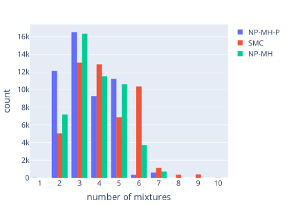
Figure 3: Histogram of the number of components for the infinite GMM; correct posterior is 3.

We first implemented two simple instances of the NP-iMCMC sampler, namely NP-MH (LABEL:app:_np-mh) and NP-MH with Persistence (LABEL:app:_lifted_np-mh) in the Turing language (Ge et al., 2018). We compared them with Turing’s built-in Sequential Monte Carlo (SMC) algorithm on an infinite Gaussian mixture model (GMM) where the number of mixture components is drawn from a normal distribution. Posterior inference is performed on 30 data points generated from a ground truth with three components. The results of ten runs with 5000 iterations each (Fig. 3) suggest that the NP-iMCMC samplers work pretty well.

5.2 Nonparametric Hamiltonian Monte Carlo

Secondly, we consider Nonparametric HMC (Mak et al., 2021b), mentioned in Ex. 2 before. We have seen how the techniques from Sec. 4 can yield nonreversible versions of NP-iMCMC inference algorithms. Here, we look at nonparametric versions of two extensions described in (Neklyudov et al., 2020): persistence (Ex. 3) and lookahead (Ex. 4). Persistence means that the previous momentum vector is reused in the next iteration. It is parametrised by $\alpha\in[0,1]$ where $\alpha=1$ means no persistence (standard HMC) and $\alpha=0$ means full persistence (no randomness added to the momentum vector). Lookahead HMC is parametrised by $K\geq 0$, which is the number of extra iterations (“look ahead”) to try before rejecting a proposed sample (so $K=0$ corresponds to standard HMC). Detailed descriptions of these algorithms and how they fit into the (Multiple Step) NP-iMCMC framework can be found in LABEL:app:_gen_np-hmc and LABEL:app:_look_ahead_np-hmc.

We evaluate these extensions of NP-HMC on the benchmarks from (Mak et al., 2021b): a model for the geometric distribution, a model involving a random walk, and an unbounded Gaussian mixture model. Note that similarly to (Mak et al., 2021b), we actually work with a discontinuous version of NP-HMC, called NP-DHMC, which is a nonparametric extension of discontinuous HMC (Nishimura et al., 2020). The discontinuous version can handle the discontinuities arising from the jumps between dimensions more efficiently. We don’t discuss it in this paper due to lack of space. However, the modifications necessary to this discontinuous version are the same as for the standard NP-HMC. Mak et al. (2021b) demonstrated the usefulness of NP-DHMC and how it can obtain better results than other general-purpose inference algorithms like Lightweight Metropolis-Hastings and Random-walk Lightweight Metropolis-Hastings. Here, we focus on the benefits of nonreversible versions of NP-DHMC, which were derived using the (Multiple Step) NP-iMCMC framework.

Table 1: Geometric distribution example: total variation difference from the ground truth, averaged over 10 runs, and standard deviation. Each run: $10^{3}$ samples, $L$ leapfrog steps, step size $\epsilon=0.1$, persistence parameter $\alpha\in\{0.5\}$.

	persistence	TVD from ground truth
$L=5$	—	$0.0524\pm 0.0069$
$L=5$	$\alpha=0.5$	$0.0464\pm 0.0074$
$L=5$	$\alpha=0.1$	$0.0461\pm 0.0083$
$L=2$	—	$0.0768\pm 0.0181$
$L=2$	$\alpha=0.5$	$0.0570\pm 0.0115$
$L=2$	$\alpha=0.1$	$0.0534\pm 0.0058$

Geometric distribution

The geometric distribution benchmark from (Mak et al., 2021b) illustrates the usefulness of persistence: we ran NP-DHMC for a step count $L\in\{2,5\}$ with and without persistence. As can be seen in Table 1, persistence usually decreases the distance from the ground truth. In fact, the configuration $L=2,\alpha=0.1$ is almost as good as $L=5$ without persistence, despite taking 2.5 times less computing time.

Figure 4: ESS for the random walk example in terms of number of samples, computed from 10 runs. Each run: $10^{3}$ samples with $L=5$ leapfrog steps of size $\epsilon=0.1$, persistence parameter $\alpha\in\{0.5,0.1\}$, and look-ahead $K\in\{1,2\}$.

Random walk

The next benchmark from (Mak et al., 2021b) models a random walk and observes the distance travelled. Fig. 4 shows the effective sample size (ESS) in terms of the number of samples drawn, comparing versions of NP-DHMC with persistence ($\alpha=0.5$) and look-ahead ($K\in\{1,2\}$). We can see again that persistence is clearly advantageous. Look-ahead ($K\in\{1,2\}$) seems to give an additional boost on top. We ran all these versions with the same computation time budget, which is why the the lines for $K=1,2$ are cut off before the others.

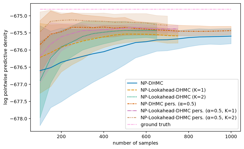
Figure 5: Gaussian mixture with Poisson prior: LPPD in terms of number of samples, averaged over 10 runs. The shaded area is one standard deviation. Each run: $10^{3}$ samples with $L=25$ leapfrog steps of size $\epsilon=0.05$, persistence parameter $\alpha=0.5$, and look-ahead $K\in\{1,2\}$.

Unbounded Gaussian mixture model

Next, we consider a Gaussian mixture model where the number of mixture components is drawn from a Poisson prior. Inference is performed on a training data set generated from a mixture of 9 components (the ground truth). We then compute the log pointwise predictive density (LPPD) on a test data set drawn from the same distribution as the training data. The LPPD is shown in Fig. 5 in terms of the number of samples. Note that again, all versions were run with the same computation budget, which is why some of the lines are cut off early. Despite this, we can see that the versions with lookahead ($K\in\{1,2\}$) converge more quickly than the versions without lookahead. Persistent direction ($\alpha=0.5$) also seems to have a (smaller) benefit.

Figure 6: Dirichlet process mixture: LPPD in terms of number of samples, averaged over 10 runs. The shaded area is one standard deviation. Each run: 150 samples with $L=20$ leapfrog steps of size $\epsilon=0.05$, persistence parameter $\alpha=0.5$, and look-ahead $K\in\{1,2\}$.

Dirichlet process mixture model

Finally, we consider a Gaussian mixture whose weights are drawn from a Dirichlet process. The rest of the setup is the same as for the Poisson prior, and the results are shown in Fig. 6. The version with persistence is worse at the start but obtains a better LPPD at the end. Look-ahead ($K\in\{1,2\}$) yields a small additional boost in the LPPD. It should be noted that the variance over the 10 runs is larger in this example than in the previous benchmarks, so the conclusion of this benchmark is less clear-cut.

6 Related work and Conclusion

Involutive MCMC and its instances

The involutive MCMC framework (Neklyudov et al., 2020; Cusumano-Towner et al., 2019; Matheos et al., 2020) can in principle be used for nonparametric models by setting $X:=\bigcup_{n\in\mathsf{\mathbb{N}}}\mathbb{X}^{n}$ and $Y:=\bigcup_{n\in\mathsf{\mathbb{N}}}\mathbb{Y}^{n}$ in Fig. 1 and defining an auxiliary kernel on $X\leadsto Y:=\bigcup_{n\in\mathsf{\mathbb{N}}}\mathbb{X}^{n}\leadsto\bigcup_{n\in\mathsf{\mathbb{N}}}\mathbb{Y}^{n}$ an involution on $X\times Y:=\bigcup_{n\in\mathsf{\mathbb{N}}}\mathbb{X}^{n}\times\mathbb{Y}^{n}$. For instance, Reversible Jump MCMC (Green, 1995) is an instance of iMCMC that works for the infinite GMM model, with the split-merge proposal (Richardson & Green, 1997) specifying when and how states can “jump” across dimensions. However, designing appropriate auxiliary kernels and involutions that enable the extension of an iMCMC sampler to nonparametric models remains challenging and model specific. By contrast, NP-iMCMC only requires the specification of involutions on the finite-dimensional space $\mathbb{X}^{n}\times\mathbb{Y}^{n}$; moreover, it provides a general procedure (via Item 3) that drives state movement between dimensions. For designers of nonparametric samplers who do not care to custom build trans-dimensional methods, we contend that NP-iMCMC is their method of choice.

The performance of NP-iMCMC and iMCMC depends on the complexity of the respective auxiliary kernels, involutions and the model in question. Take iGMM for example. RJMCMC with the split-merge proposal which computes the weight, mean, and variance of the new component(s) would be slower than NP-MH, an instance of NP-iMCMC with a computationally light involution (a swap), but more efficient than NP-HMC, an instance of (Multiple Step) NP-iMCMC with the computationally heavy leapfrog integrator as involution.

Trans-dimensional samplers

A standard MCMC algorithm for universal PPLs is the Lightweight Metropolis-Hastings algorithm (LMH) (Yang et al., 2014; Tolpin et al., 2015; Ritchie et al., 2016). Widely implemented in several universal PPLs (Anglican, Venture, Gen, and Web PPL), LMH performs single-site updates on the current sample and re-executes the program from the resampling point.

Divide, Conquer, and Combine (DCC) (Zhou et al., 2020) is an inference algorithm that is applicable to probabilistic programs that use branching and recursion. A hybrid algorithm, DCC solves the problem of designing a proposal that can efficiently transition between configurations by performing local inferences on submodels, and returning an appropriately weighted combination of the respective samples.

Mak et al. (2021b) have recently introduced Nonparametric Hamiltonian Monte Carlo (NP-HMC), which generalises HMC to nonparametric models. As we’ve seen, NP-HMC is an instantiation of (Multiple Step) NP-iMCMC.

Conclusion

We have introduced the nonparametric involutive MCMC algorithm as a general framework for designing MCMC algorithms for models expressible in a universal PPL, and provided a correctness proof. To demonstrate the relative ease of make-to-order design of nonparametric extensions of existing MCMC algorithms, we have constructed several new algorithms, and demonstrated empirically that the expected features and statistical properties are preserved.

[sections] [sections]l1

Appendix A Statistical PCF

In this section, we present a functional probabilistic programming language (PPL) with (stochastic) branching and recursion, and its operational semantics. We also define what it means for a program to be almost surely terminating and integrable. We conclude the section by showing that a broad class of programs satisfies the assumptions for the NP-iMCMC inference algorithm described in Sec. 3.

A.1 Syntax

Statistical PCF (SPCF) is a statistical probabilistic extension of the call-by-value PCF (Scott, 1993; Sieber, 1990) with the reals and Booleans as the ground types. The terms and part of the typing system of SPCF are presented in Fig. 7.

SPCF has three probabilistic constructs:

1. The continuous sampler $\mathsf{normal}$ draws from the standard Gaussian distribution $\mathcal{N}$ with mean $0$ and variance $1$.

2. The discrete sampler $\mathsf{coin}$ is a fair coin (formally $\mathsf{coin}$ draws from the Bernoulli distribution $\mathsf{Bern}(0.5)$ with probability $0.5$).

3. The scoring construct $\mathsf{score}(M)$ enables conditioning on observed data by multiplying the weight of the current execution with the real number denoted by $M$.

Remark A.1 (Continuous Sampler).

The continuous sampler in most PPLs (Culpepper & Cobb, 2017; Wand et al., 2018; Ehrhard et al., 2018; Vákár et al., 2019; Mak et al., 2021a) draw from the standard uniform distribution $\mathcal{U}$ with endpoints $0$ and $1$. However, we decided against $\mathcal{U}$ since its support is not the whole of $\mathbb{R}$, which is a common target space for inference algorithms (e.g. Hamiltonian Monte Carlo (HMC) inference algorithm). Instead our continuous sampler draws from the standard normal distribution $\mathcal{N}$ which has the whole of $\mathbb{R}$ as its support. This design choice does not restrict nor extend our language as we will see in Ex. 6.

Remark A.2 (Discrete Sampler).

Like (Danos & Ehrhard, 2011; Ścibior et al., 2018), we choose the fair coin as our discrete sampler for its simplicity. However, as shown in Ex. 7, this is not limiting. (Ehrhard et al., 2014), for example, samples from the discrete uniform distribution.

Types (typically denoted $\sigma,\tau$) and terms (typically $M,N,L$):

$$\sigma,\tau ::=\mathsf{R}\mid\mathsf{B}\mid\sigma\Rightarrow\tau$$

$$M,N,L ::=\underline{r}\mid\underline{a}\mid\underline{f}(M_{1},\dots,M_{\ell})$$ (Constants and functions)

$$\mid y\mid\lambda y.M\mid M\,N$$ (Higher-order)

$$\mid\mathsf{if}(L,M,N)\mid\mathsf{Y}{M}$$ (Branching and recursion)

$$\mid\mathsf{normal}\mid\mathsf{coin}\mid\mathsf{score}(M)$$ (Probabilistic)

Typing system:

   $$a\in\mathbb{2} \Gamma\vdash\underline{a}:\mathsf{B} \{\Gamma\vdash M_{i}:\mathsf{R}\}_{i=1}^{n} \{\Gamma\vdash N_{j}:\mathsf{B}\}_{j=1}^{m} f:\mathbb{R}^{n}\times\mathbb{2}^{m}\rightharpoonup G \Gamma\vdash\underline{f}{(M_{1},\dots,M_{n},N_{1},\dots,N_{m})}:\begin{cases}\mathsf{R}&\text{if }G=\mathbb{R}\\ \mathsf{B}&\text{if }G=\mathbb{2}\end{cases}$$                                                

  $$\Gamma\vdash L:\mathsf{B} \Gamma\vdash M:\sigma \Gamma\vdash N:\sigma \Gamma\vdash\mathsf{if}(L,M,N):\sigma \Gamma\vdash M:(\sigma\Rightarrow\tau)\Rightarrow(\sigma\Rightarrow\tau) \Gamma\vdash\mathsf{Y}{M}:\sigma\Rightarrow\tau$$                                                             

          $$4 \Gamma\vdash\mathsf{normal}:\mathsf{R} 4 \Gamma\vdash\mathsf{coin}:\mathsf{B} \Gamma\vdash M:\mathsf{R} \Gamma\vdash\mathsf{score}(M):\mathsf{R}$$                                                    

Figure 7: Syntax of SPCF, where $r,q,p\in\mathbb{R}$, $a,b\in\mathbb{2}$, $x,y,z$ are variables, and $f,g,h$ ranges over a set $\mathcal{F}$ of primitive functions.

Following the convention, the set of all terms is denoted as $\Lambda$ with meta-variables $M,N,L$, the set of free variables of a term $M$ is denoted as $\mathsf{FV}(M)$ and the set of all closed terms is denoted as $\Lambda^{0}$. In the interest of readability, we sometimes use pseudocode in the style of ML (e.g. Ex. 5) to express SPCF terms.

Example 5.

let rec f x = if coin then f(x+normal) else x in f 0 is a simple program which keeps tossing a coin and sampling from the normal distribution until the first coin failure, upon which it returns the sum of samples from the normal distribution.

A.2 Primitive Functions

Primitive functions play an important role in the expressiveness of SPCF. To be concise, we only consider partial, measurable functions of types $\mathbb{R}^{n}\times\mathbb{2}^{m}\rightharpoonup\mathbb{R}$ or $\mathbb{R}^{n}\times\mathbb{2}^{m}\rightharpoonup\mathbb{2}$ for some $n,m\in\mathsf{\mathbb{N}}$. Examples of these primitives include addition $+$, division $/$, comparison $<$ and equality $=$. As we will see in Ex. 6 and 7, it is important that the cumulative distribution functions (cdf) and probability density functions (pdf) of distributions are amongst the primitives in $\mathcal{F}$. However, we do not require all measurable functions to be primitives, unlike (Staton et al., 2016; Staton, 2017).

Example 6.

1. Let cdfnormal be the cdf of the standard normal distribution. Then, the standard uniform distribution with endpoints $0$ and $1$ can be described as uniform = cdfnormal(normal).

2. Any distribution with an inverse cdf f in the set of primitives can be described as f(uniform). For instance, the inverse cdf of the exponential distribution (with rate $1$) is $f(p):=-\ln(1-p)$ and hence -ln(1-uniform) describes the distribution.

3. The Poisson distribution can be specified using the uniform distribution ((Devroye, 1986)) as follows.

   ⬇

   let rec f x p s = if s < uniform then f (x+1) (p*rate/x) (s+p) else x

   in f 0 p p

Example 7.

It might be beneficial for some inference algorithm if discrete distributions are specified using discrete random variables. Hence, we show how different discrete distributions can be specified by our discrete sampler coin.

1. The Bernoulli distribution with probability $p\in[0,1]\cap\mathbb{D}$, where $\mathbb{D}:=\{\frac{n}{2^{m}}\mid n,m\in\mathsf{\mathbb{N}}\}$ is the set of all Dyadic numbers, can be specified by

   ⬇

   if p = 1 then True else

   if p < 0.5 then

   if coin then bern(2*p) else False

   else

   if coin then True else bern(2*(p-0.5))

2. The geometric distribution with rate $p\in[0,1]\cap\mathbb{D}$ can be specified by

3. The binomial distribution with $n\in\mathsf{\mathbb{N}}$ trails and probability $p\in[0,1]\cap\mathbb{D}$ can be specified by bin(n,p) = sum([1 for i in range(n) if bern(p)]).

4. Let pdfPio and pdfgeo be the pdfs of the Poisson and geometric distributions respectively. Then, the Poisson distribution can be described by

   ⬇

   score(pdfPoi(rate,n)/pdfgeo(0.5,n));

   return n

A.3 Church Encodings

We can represent pairs and lists in SPCF using Church encoding as follows:

$$\mathsf{Pair}(\sigma,\tau) :=\sigma\to\tau\to(\sigma\to\tau\to\mathsf{R})\to\mathsf{R} \mathsf{List}(\sigma) :=(\sigma\to\mathsf{R}\to\mathsf{R})\to(\mathsf{R}\to\mathsf{R})$$

$$\langle M,N\rangle \equiv\lambda z.z\,M\,N [M_{1},\dots,M_{\ell}] \equiv\lambda fx.f\,M_{1}(f\,M_{2}\dots(f\,M_{\ell}\,\underline{0}))$$

Moreover standard primitives on pairs and lists, such as projection, len, append and sum, can be defined easily.

A.4 Operational Semantics

A.4.1 Trace Space

Since $\mathsf{normal}$ samples from the standard normal distribution $\mathcal{N}$ and $\mathsf{coin}$ from the Bernoulli distribution $\mathsf{Bern}(0.5)$, the sample space of SPCF is the union of the measurable spaces of $\mathbb{R}$ and $\mathbb{2}$. Formally it is the measurable space with set $\mathbb{\Omega}:=\mathbb{R}\cup\mathbb{2}$, $\sigma$-algebra $\Sigma_{\mathbb{\Omega}}:=\{V\cup W\mid V\in\mathcal{B},W\in\Sigma_{\mathbb{2}}\}$ and measure $\mu_{\mathbb{\Omega}}(V\cup W):=\mathcal{N}(V)+\mathsf{Bern}(0.5)(W)$. We denote the product of $n$ copies of the sample space as $(\mathbb{\Omega}^{n},\Sigma_{\mathbb{\Omega}^{n}},\mu_{\mathbb{\Omega}^{n}})$ and call it the $n$-dimensional sample space.

A trace is a record of the values sampled in the course of an execution of a SPCF term. Hence, the trace space is the union of sample spaces of varying dimension. Formally it is the measurable space with set $\mathbb{T}:=\bigcup_{n\in\mathsf{\mathbb{N}}}\mathbb{\Omega}^{n}$, $\sigma$-algebra $\Sigma_{\mathbb{T}}:=\{\bigcup_{n\in\mathsf{\mathbb{N}}}U_{n}\mid U_{n}\in\Sigma_{\mathbb{\Omega}^{n}}\}$ and measure $\mu_{\mathbb{T}}(\bigcup_{n\in\mathsf{\mathbb{N}}}U_{n})=\sum_{n\in\mathsf{\mathbb{N}}}\mu_{\mathbb{\Omega}^{n}}(U_{n})$. We present traces as lists, e.g. $[-0.2,\mathsf{T},\mathsf{T},3.1,\mathsf{F}]$ and $[]$.

Remark A.3.

Another way of recording the sampled value in a run of a SPCF term is to have separate records for the values of the continuous and discrete samples. In this case, the trace space will be the set $\bigcup_{n\in\mathsf{\mathbb{N}}}\mathbb{R}^{n}\times\bigcup_{m\in\mathsf{\mathbb{N}}}\mathbb{2}^{m}$. We find separating the continuous and discrete samples unnecessarily complex for our purposes and hence follow the more conventional definition of trace space.

A.4.2 Small-step Reduction

Values (typically denoted $V$), redexes (typically $R$) and evaluation contexts (typically $E$):

$$V ::=\underline{r}\mid\underline{a}\mid\lambda y.M$$

$$R ::=\underline{f}(\underline{c_{1}},\dots,\underline{c_{\ell}})\mid(\lambda y.M)\,V\mid\mathsf{if}(\underline{a},M,N)\mid\mathsf{Y}{(\lambda y.M)}$$

$$\mid\mathsf{normal}\mid\mathsf{coin}\mid\mathsf{score}(\underline{r})$$

$$E ::=[]\mid E\,M\mid(\lambda y.M)\,E\mid\mathsf{if}(E,M,N)\mid\underline{f}(\underline{c_{1}},\dots,\underline{c_{i-1}},E,M_{i+1},\dots,M_{\ell})\mid\mathsf{Y}{E}$$

$$\mid\mathsf{score}(E)$$

Redex contractions:

$$\langle\underline{f}(\underline{c_{1}},\dots,\underline{c_{\ell}}),w,\boldsymbol{t}\rangle \longrightarrow\begin{cases}\langle\underline{f(c_{1},\dots,c_{\ell})},w,\boldsymbol{t}\rangle&\text{if }(c_{1},\dots,c_{\ell})\in\mathsf{Dom}(f),\\ \mathsf{fail}&\text{otherwise}\end{cases}$$

$$\langle(\lambda y.M)\,V,w,\boldsymbol{t}\rangle \longrightarrow\langle M[V/y],w,\boldsymbol{t}\rangle$$

$$\langle\mathsf{if}(\underline{a},M,N),w,\boldsymbol{t}\rangle \longrightarrow\begin{cases}\langle M,w,\boldsymbol{t}\rangle&\text{if }a,\\ \langle N,w,\boldsymbol{t}\rangle&\text{otherwise}\end{cases}$$

$$\langle\mathsf{Y}{(\lambda y.M)},w,\boldsymbol{t}\rangle \longrightarrow\langle\lambda z.M[\mathsf{Y}{(\lambda y.M)}/y]\,z,w,\boldsymbol{t}\rangle z$$ (for fresh variable )

$$\langle\mathsf{normal},w,\boldsymbol{t}\rangle \longrightarrow\langle\underline{r},w,t\mathbin{+\mkern-8.0mu+}[r]\rangle r\in\mathbb{R}$$ (for some )

$$\langle\mathsf{coin},w,\boldsymbol{t}\rangle \longrightarrow\langle\underline{a},w,t\mathbin{+\mkern-8.0mu+}[a]\rangle a\in\mathbb{2}$$ (for some )

$$\langle\mathsf{score}(\underline{r}),w,\boldsymbol{t}\rangle \longrightarrow\begin{cases}\langle\underline{r},r\cdot w,\boldsymbol{t}\rangle&\text{if }r>0,\\ \mathsf{fail}&\text{otherwise.}\end{cases}$$

Evaluation contexts:

      $$\langle R,w,\boldsymbol{t}\rangle\longrightarrow\langle\Delta,w^{\prime},t^{\prime}\rangle \langle E[R],w,\boldsymbol{t}\rangle\longrightarrow\langle E[\Delta],w^{\prime},t^{\prime}\rangle \langle R,w,\boldsymbol{t}\rangle\longrightarrow\mathsf{fail} \langle E[R],w,\boldsymbol{t}\rangle\longrightarrow\mathsf{fail}$$                      

Figure 8: Small-step reduction of SPCF, where $r,q,p\in\mathbb{R}$, $a,b\in\mathbb{2}$, $c\in\mathbb{R}\cup\mathbb{2}$, $x,y,z$ are variables, and $f,g,h$ ranges over the set $\mathcal{F}$ of primitive functions.

The small-step reduction of SPCF terms can be seen as a rewrite system of configurations, which are triples of the form $\langle M,w,\boldsymbol{t}\rangle$ where $M$ is a closed SPCF term, $w>0$ is a weight, and $\boldsymbol{t}\in\mathbb{T}$ a trace, as defined in Fig. 8.

In the rule for $\mathsf{normal}$, a random value $r\in\mathbb{R}$ is generated and recorded in the trace, while the weight remains unchanged: even though the program samples from a normal distribution, the weight does not factor in Gaussian densities as they are already accounted for by $\mu_{\mathbb{T}}$. Similarly, in the rule for $\mathsf{coin}$, a random boolean $a\in\mathbb{2}$ is sampled and recorded in the trace with an unchanged weight. In the rule for $\mathsf{score}(\underline{r})$, the current weight is multiplied by $r\in\mathbb{R}$: typically this reflects the likelihood of the current execution given some observed data. Similar to (Borgström et al., 2016) we reduce terms which cannot be reduced in a reasonable way (i.e. scoring with nonpositive constants or evaluating functions outside their domain) to $\mathsf{fail}$.

We write $\longrightarrow^{+}$ for the transitive closure and $\longrightarrow^{*}$ for the reflexive and transitive closure of the small-step reduction.

A.4.3 Value and Weight Functions

Following (Borgström et al., 2016), we view the set $\Lambda$ of all SPCF terms as $\bigcup_{n,m\in\mathsf{\mathbb{N}}}(\mathsf{SK}_{n,m}\times\mathbb{R}^{n}\times\mathbb{2}^{m})$ where $\mathsf{SK}_{n,m}$ is the set of SPCF terms with exactly $n$ real-valued and $m$ boolean-valued place-holders. The measurable space of terms is equipped with the $\sigma$-algebra $\Sigma_{\Lambda}$ that is the Borel algebra of the countable disjoint union topology of the product topology of the discrete topology on $\mathsf{SK}_{n,m}$, the standard topology on $\mathbb{R}^{n}$ and the discrete topology on $\mathbb{2}^{m}$. Similarly the subspace $\Lambda^{0}_{v}$ of closed values inherits the Borel algebra on $\Lambda$.

Let $M$ be a closed SPCF term. Its value function $\mathsf{value}_{M}:\mathbb{T}\to\Lambda^{0}_{v}\cup\{\bot\}$ returns, given a trace, the output value of the program, if the program terminates in a value. Its weight function $\mathsf{weight}_{M}:\mathbb{T}\to[0,\infty)$ returns the final weight of the corresponding execution. Formally:

$$\begin{array}[]{c}\mathsf{value}_{M}(t):=\begin{cases}V&\hbox{if $\langle M,1,[]\rangle\longrightarrow^{*}\langle V,w,\boldsymbol{t}\rangle$}\\ \bot&\text{otherwise.}\end{cases}\end{array}\quad\begin{array}[]{c}\mathsf{weight}_{M}(t):=\begin{cases}w&\hbox{if $\langle M,1,[]\rangle\longrightarrow^{*}\langle V,w,\boldsymbol{t}\rangle$}\\ 0&\text{otherwise.}\end{cases}\end{array}$$

It follows readily from (Borgström et al., 2016) that the functions $\mathsf{value}_{M}$ and $\mathsf{weight}_{M}$ are measurable.

Finally, every closed SPCF term $M$ has an associated value measure $\langle\!\langle{M}\rangle\!\rangle$ on $\Lambda^{0}_{v}$ given by

$${\langle\!\langle{M}\rangle\!\rangle}:{\Sigma_{\Lambda^{0}_{v}}} \longrightarrow{[0,\infty)}$$

$$U \longmapsto\int_{{{\mathsf{value}_{M}}^{-1}}(U)}\ {\mathsf{weight}_{M}}\ \textrm{d}{\mu_{\mathbb{T}}}$$

Remark A.4.

A trace is in the support of the weight function if and only if the value function returns a (closed) value when given this trace. i.e. $\text{Supp}(\mathsf{weight}_{M})={{\mathsf{value}_{M}}^{-1}}(\Lambda^{0})$ for all closed SPCF term $M$.

Remark A.5.

The weight function defined here is the density of the target distribution from which an inference algorithm typically samples. In this work, we call it the weight function when considering semantics following (Culpepper & Cobb, 2017; Vákár et al., 2019; Mak et al., 2021a), and call it density function when discussing inference algorithms following (Zhou et al., 2019, 2020; Cusumano-Towner et al., 2020).

A.5 Tree Representable Functions

We consider a necessary condition for the weight function of closed SPCF terms which would help us in designing inference algorithms for them. Note that not every function of type $\mathbb{T}\to[0,\infty)$ makes sense as a weight function. Consider the program let rec f x = if coin then f(x+normal) else x in f 0 in Ex. 5. This program executes successfully with the trace $[\mathsf{T},0.5,\mathsf{F}]$. This immediately tells us that upon sampling $\mathsf{T}$ and $0.5$, there must be a sample following them, and this third sample must be a boolean. In other words, the program does not terminate with any proper prefix of $[\mathsf{T},0.5,\mathsf{F}]$ such as $[\mathsf{T},0.5]$, nor any traces of the form $[\mathsf{T},0.5,r]$ for $r\in\mathbb{R}$.

Hence, we consider measurable functions $w:\mathbb{T}\to[0,\infty)$ satisfying

• prefix property: whenever $\boldsymbol{t}\in\text{Supp}^{n}(w)$ then for all $k<n$, we have $t^{1\dots k}\not\in\text{Supp}^{k}(w)$; and

• type property: whenever $\boldsymbol{t}\in\text{Supp}^{n}(w)$ then for all $k<n$ and for all $t\in\mathbb{\Omega}\setminus\mathsf{Type}({\boldsymbol{t}}^{k+1})$ we have $\boldsymbol{t}^{1\dots k}\mathbin{+\mkern-8.0mu+}[t]\not\in\text{Supp}^{k+1}(w)$.

They are called tree representable (TR) functions (Mak et al., 2021b) because any such function $w$ can be represented as a (possibly) infinite but finitely branching tree, which we call program tree.

This is exemplified in Fig. 9 (left), where a hexagon node denotes an element of the input of type $\mathbb{\Omega}$; a triangular node gives the condition for $\boldsymbol{t}\in\text{Supp}^{n}(w)$ (with the left, but not the right, child satisfying the condition); and a leaf node gives the result of the function on that branch. Any branch (i.e. path from root to leaf) in a program tree of $w$ represents a set of finite sequences $[t_{1},\dots,t_{n}]$ in $\text{Supp}(w)$. In fact, every program tree of a TR function $w$ specifies a countable partition of $\text{Supp}(w)$ via its branches. The prefix property guarantees that for each TR function $w$, there are program trees of the form in Fig. 9 representing $w$.

The program tree of $M$ is depicted in Fig. 9 (right), where a circular node denotes a real-valued input and a squared node denotes a boolean-valued input.

Figure 9: Program tree of a tree representable function $w$

The following proposition ties SPCF terms and TR functions together.

Proposition A.6.

Every closed SPCF term has a tree representable weight function.

We will see in Sec. 3 how the TR functions, in particular the prefix property, is instrumental in the design of the inference algorithm.

A.6 Almost Sure Termination and Integrability

Definition A.7.

We say a SPCF term $M$ terminates almost surely if $M$ is closed and $\mu_{\mathbb{T}}(\{\boldsymbol{t}\in\mathbb{T}\mid\exists V,w\,.\,\langle M,1,[]\rangle\longrightarrow^{*}\langle V,w,\boldsymbol{t}\rangle\})=1$.

We denote the set of terminating traces as $\mathbb{T}_{\mathsf{ter}}:=\{\boldsymbol{t}\in\mathbb{T}\mid\exists V,w\,.\,\langle M,1,[]\rangle\longrightarrow^{*}\langle V,w,\boldsymbol{t}\rangle\}$.

Remark A.8.

The set of traces on which a closed SPCF term $M$ terminates, i.e. $\{\boldsymbol{t}\in\mathbb{T}\mid\exists V,w\,.\,\langle M,1,[]\rangle\longrightarrow^{*}\langle V,w,\boldsymbol{t}\rangle\}$, can be understood as the support of its weight function $\text{Supp}(\mathsf{weight}_{M})$, or as discussed in Rem. A.4, the traces on which the value function returns a value, i.e. ${{\mathsf{value}_{M}}^{-1}}(\Lambda^{0}_{v})$. Hence, $M$ almost surely terminates if and only if $\mu_{\mathbb{T}}(\text{Supp}(\mathsf{weight}_{M}))=\mu_{\mathbb{T}}({{\mathsf{value}_{M}}^{-1}}(\Lambda^{0}_{v}))=1$.

Definition A.9.

Following (Mak et al., 2021a), we say a trace $\boldsymbol{t}\in\mathbb{T}$ is maximal w.r.t. a closed term $M$ if there exists a term $N$, weight $w$ where $\langle M,1,[]\rangle\longrightarrow^{*}\langle N,w,\boldsymbol{t}\rangle$ and for all $\boldsymbol{t}^{\prime}\in\mathbb{T}\setminus\{[]\}$ and all terms $N^{\prime}$, $\langle N,w,\boldsymbol{t}\rangle\not\longrightarrow^{*}\langle N^{\prime},w^{\prime},\boldsymbol{t}\mathbin{+\mkern-8.0mu+}\boldsymbol{t}^{\prime}\rangle$.

We denote the set of maximal traces as $\mathbb{T}_{\mathsf{max}}$.

Proposition A.10 ((Mak et al., 2021a), Lemma 9).

A closed term $M$ is almost surely terminating if $\mu_{\mathbb{T}}(\mathbb{T}_{\mathsf{max}}\setminus\mathbb{T}_{\mathsf{ter}})=0$.

Proposition A.11.

The value measure $\langle\!\langle{M}\rangle\!\rangle$ of a closed almost surely terminating SPCF term $M$ which does not contain $\mathsf{score}(\cdot)$ as a subterm is probabilistic.

Definition A.12.

We say a SPCF term $M$ is integrable if $M$ is closed and its value measure is finite, i.e. $\langle\!\langle{M}\rangle\!\rangle(\Lambda^{0}_{v})<\infty$;

Proposition A.13.

An integrable term has an integrable weight function.

Example 8.

Now we look at a few examples in which we show that almost surely termination and integrability identify two distinct sets of SPCF terms.

1. The term $M_{1}$ defined as let rec f x = if coin then f (x+1) else x in score(2**(f 0)) almost surely terminates since it only diverges on the infinite trace $[\mathsf{F},\mathsf{F},\dots]$ which has zero probability. However, it is not integrable as the value measure applied to all closed values $\langle\!\langle{M_{1}}\rangle\!\rangle(\Lambda^{0}_{v})=\int_{\{[\mathsf{T},\dots,\mathsf{T},\mathsf{F}]\}}\ {\mathsf{weight}_{M_{1}}}\ \textrm{d}{\mu_{\mathbb{T}}}=\sum_{n=0}^{\infty}\int_{\{[T]^{n}\mathbin{+\mkern-8.0mu+}[\mathsf{F}]\}}\ {\mathsf{weight}_{M_{1}}}\ \textrm{d}{\mu_{\mathbb{2}^{n}}}=\sum_{n=0}^{\infty}(\frac{1}{2})^{n+1}\cdot 2^{n}=\sum_{n=0}^{\infty}\frac{1}{2}$ is infinite.

2. Consider the term $M_{2}$ defined as if coin then Y (lambda x:x) 0 else 1. Since it reduces to a diverging term, namely Y (lambda x:x) 0, with non-zero probability, it does not terminate almost surely. However, it is integrable, since $\langle\!\langle{M_{2}}\rangle\!\rangle(\Lambda^{0}_{v})=\int_{\{[\mathsf{F}]\}}\ {\mathsf{weight}_{M_{2}}}\ \textrm{d}{\mu_{\mathbb{T}}}=\frac{1}{2}<\infty$.

3. The term $M_{3}$ defined as $\mathsf{if}(\mathsf{coin},M_{1},M_{2})$ is neither almost surely terminating nor integrable, since $M_{1}$ is not integrable and $M_{2}$ is not almost surely terminating.

4. All terms considered previously in Ex. 5, 6 and 7 are both almost surely terminating and integrable.

Appendix B Hybrid Nonparametric Involutive MCMC and its Correctness

In this section, we present the Hybrid Nonparametric Involutive Markov chain Monte Carlo (Hybrid NP-iMCMC), an inference algorithm that simulates the probabilistic model specified by a given SPCF program that may contains both discrete and continuous samplers.

To start, we detail the Hybrid NP-iMCMC inference algorithm: its state space, conditions on the inputs and steps to generate the next sample; and study how the sampler moves between states of varying dimensions and returns new samples of a nonparametric probabilistic program. We then give an implementation of Hybrid NP-iMCMC in SPCF and demonstrate how the Hybrid NP-iMCMC method extends the MH sampler. Last but not least, we conclude with a discussion on the correctness of Hybrid NP-iMCMC.

B.1 State Spaces

A state in the Hybrid NP-iMCMC algorithm is a pair $(\boldsymbol{x},\boldsymbol{v})$ of equal dimension (but not necessarily equal length) parameter and auxiliary variables. The parameter variable $\boldsymbol{x}$ is used to store traces and the auxiliary variable $\boldsymbol{v}$ is used to record randomness. Both variables are vectors of entropies, i.e. Real-Boolean pairs. This section gives the formal definitions of the entropy, parameter and auxiliary variables and the state, in preparation for the discussion of the Hybrid NP-iMCMC sampler.

B.1.1 Entropy Space

As shown in App. A, the reduction of a SPCF program is determined by the input trace $\boldsymbol{t}\in\mathbb{T}:=\bigcup_{n\in\mathsf{\mathbb{N}}}(\mathbb{R}\cup\mathbb{2})^{n}$, a record of drawn values in a particular run of the program. Hence in order to simulate a probabilistic model described by a SPCF program, the Hybrid NP-iMCMC sampler should generate Markov chains on the trace space. However traversing through the trace space is a delicate business because the positions and numbers of discrete and continuous values in a trace given by a SPCF program may vary. (Consider if coin: normal else: coin.)

Instead, we pair each value ${\boldsymbol{t}}^{i}$ in a trace $\boldsymbol{t}$ with a random value $t$ of the other type to make a Real-Boolean pair $({\boldsymbol{t}}^{i},t)$ (or $(t,{\boldsymbol{t}}^{i})$). For instance, the trace $[\mathsf{T},-3.1]$ can be made into a Real-Boolean vector $[(1.5,\mathsf{T}),(-3.1,\mathsf{T})]$ with randomly drawn values $1.5$ and $\mathsf{T}$. Now, the position of discrete and continuous random variables does not matter and the number of discrete and continuous random variables are fixed in each vector.

We call a Real-Boolean pair an entropy and define the entropy space ${\mathbb{E}}$ to be the product space $\mathbb{R}\times\mathbb{2}$ of the Borel measurable space and the Boolean measurable space, equipped with the $\sigma$-algebra $\Sigma_{{\mathbb{E}}}:=\sigma\big{(}\{R\times B\mid R\in\mathcal{B},B\in\Sigma_{\mathbb{2}}\}\big{)}$, and the product measure $\mu_{{\mathbb{E}}}:={\mathcal{N}}\times{\mu_{\mathbb{2}}}$ where ${\mu_{\mathbb{2}}}:=\mathsf{Bern}(0.5)$. Note the Radon-Nikodym derivative $\varphi_{{\mathbb{E}}}$ of $\mu_{{\mathbb{E}}}$ can be defined as $\varphi_{{\mathbb{E}}}(r,a):=\frac{1}{2}\varphi(r)$. A $n$-length entropy vector is then a vector of $n$ entropies, formally an element in the product measurable space $({{\mathbb{E}}^{n}},\Sigma_{{\mathbb{E}}^{n}})$. We write $|{\boldsymbol{x}}|$ to mean the length of the entropy vector $\boldsymbol{x}$.

As mentioned earlier, the parameter variable of a state is an entropy vector that stores traces. Hence, it would be useless if a unique trace cannot be restored from an entropy vector. We found that such a recovery is possible if the trace is in the support of a tree representable function.

Say we would like to recover the trace $\hat{\boldsymbol{t}}$ that is used to form the entropy vector $\boldsymbol{x}$ by pairing each value in the trace with a random value of the other type. First we realise that traces can be made by selecting either the Real or Boolean component of each pair in a prefix of $\boldsymbol{x}$. For example, traces like $[]$, $[\mathsf{T}]$, $[-0.2]$, $[\mathsf{T},2.9]$ and $[-0.2,\mathsf{T},\mathsf{F}]$ can be made from the entropy vector $[(-0.2,\mathsf{T}),(2.9,\mathsf{T}),(1.3,\mathsf{F})]$. We call these traces instances of the entropy vector. Formally, a trace $\boldsymbol{t}\in\mathbb{T}$ is an instance of an entropy vector $\boldsymbol{x}\in{\mathbb{E}}^{n}$ if $|{\boldsymbol{t}}|\leq n$ and ${\boldsymbol{t}}^{i}\in\{r,a\mid(r,a)={\boldsymbol{x}}^{i}\}$ for all $i=1,\dots,|{\boldsymbol{t}}|$. We denote the set of all instances of $\boldsymbol{x}$ as $\mathsf{instance}(\boldsymbol{x})\subseteq\mathbb{T}$. Then, the trace $\hat{\boldsymbol{t}}$ must be an instance of $\boldsymbol{x}$. Moreover, if we can further assume that $\hat{\boldsymbol{t}}$ is in the support of a tree representable function, then Prop. B.1 says we can uniquely identify $\hat{\boldsymbol{t}}$ amongst all instances of $\boldsymbol{x}$.

Proposition B.1.

There is at most one (unique) trace that is both an instance of an entropy vector and in the support of a tree representable function.

Finally, we consider differentiability on the multi-dimensional entropy space. We say a function $f:{\mathbb{E}}^{k_{1}}\to{\mathbb{E}}^{k_{2}}$ is differentiable almost everywhere if for all $\boldsymbol{i}\in\mathbb{2}^{k_{1}}$, $\boldsymbol{j}\in\mathbb{2}^{k_{2}}$, the partial function $f_{{\boldsymbol{i}}\to{\boldsymbol{j}}}:\mathbb{R}^{k_{1}}\to\mathbb{R}^{k_{2}}$ where

$$f_{{\boldsymbol{i}}\to{\boldsymbol{j}}}(\boldsymbol{r})=\boldsymbol{q}\qquad\iff\qquad f(\mathsf{zip}(\boldsymbol{r},\boldsymbol{i}))=(\mathsf{zip}(\boldsymbol{q},\boldsymbol{j}))$$

is differentiable almost everywhere on its domain $\mathsf{Dom}(f_{{\boldsymbol{i}}\to{\boldsymbol{j}}}):=\{\boldsymbol{r}\in\mathbb{R}^{k_{1}}\mid\exists\boldsymbol{q}\in\mathbb{R}^{k_{2}}\ .\ f(\mathsf{zip}(\boldsymbol{r},\boldsymbol{i}))=(\mathsf{zip}(\boldsymbol{q},\boldsymbol{j}))\}$. The Jacobian of $f$ on $(\mathsf{zip}(\boldsymbol{r},\boldsymbol{i}))$ is given by ${\nabla f_{{\boldsymbol{i}}\to{\boldsymbol{j}}}}(\boldsymbol{r})$, if it exists.

B.1.2 Parameter Space

A parameter variable $\boldsymbol{x}$ of dimension $n$ is an entropy vector of length $\iota_{{\mathbb{X}}}(n)$ where $\iota_{{\mathbb{X}}}:\mathsf{\mathbb{N}}\to\mathsf{\mathbb{N}}$ is a strictly monotone map. For instance, the parameter variable $\boldsymbol{x}:=[(-0.2,\mathsf{T}),(2.9,\mathsf{T}),(1.3,\mathsf{F})]$ is of dimension two if $\iota_{{\mathbb{X}}}(n):=n+1$, and dimension three if $\iota_{{\mathbb{X}}}(n):=n$. We write $\dim(\boldsymbol{x})$ to mean the dimension of $\boldsymbol{x}$ and $|{\boldsymbol{x}}|$ to mean the length of $\boldsymbol{x}$. Hence, $\dim(\boldsymbol{x})\leq|{\boldsymbol{x}}|$ and $\iota_{{\mathbb{X}}}(\dim(\boldsymbol{x}))=|{\boldsymbol{x}}|$. We extend the notion of dimension to traces and say a trace $\boldsymbol{t}\in\mathbb{T}$ has dimension $n$ if $|{\boldsymbol{t}}|=\iota_{{\mathbb{X}}}(n)$. Importantly, we assume that every trace in the support of $w$ has a dimension (w.r.t. $\iota_{{\mathbb{X}}}$), i.e. $\text{Supp}(w)=\bigcup_{n\in\mathsf{\mathbb{N}}}\text{Supp}^{\iota_{{\mathbb{X}}}{(n)}}(w)$.

Formally, the $n$-dimensional parameter space $({{\mathbb{X}}^{({n})}},\Sigma_{{{\mathbb{X}}^{({n})}}})$ is the product of $\iota_{{\mathbb{X}}}(n)$ copies of the entropy space $({\mathbb{E}},\Sigma_{{\mathbb{E}}})$ and the base measure $\mu_{{{\mathbb{X}}^{({n})}}}$ on ${{\mathbb{X}}^{({n})}}$ is the product of $\iota_{{\mathbb{X}}}(n)$ copies of the entropy measure $\mu_{{\mathbb{E}}}$ with the Radon-Nikodym derivative $\varphi_{{{\mathbb{X}}^{({n})}}}$. For ease of reference, we write $({\mathbb{X}},\Sigma_{{\mathbb{X}}},\mu_{{\mathbb{X}}})$ for the one-dimensional parameter space.

B.1.3 Auxiliary Space

Similarly, an auxiliary variable $\boldsymbol{v}$ of dimension $n$ is an entropy vector of length $\iota_{{\mathbb{Y}}}(n)$ where $\iota_{{\mathbb{Y}}}:\mathsf{\mathbb{N}}\to\mathsf{\mathbb{N}}$ is a strictly monotone map. The $n$-dimensional auxiliary space $({{\mathbb{Y}}^{({n})}},\Sigma_{{{\mathbb{Y}}^{({n})}}})$ is the product of $\iota_{{\mathbb{Y}}}(n)$ copies of the entropy space $({\mathbb{E}},\Sigma_{{\mathbb{E}}})$ and the base measure $\mu_{{{\mathbb{Y}}^{({n})}}}$ on ${{\mathbb{Y}}^{({n})}}$ is the product of $\iota_{{\mathbb{Y}}}(n)$ copies of the entropy measure $\mu_{{\mathbb{E}}}$ with the Radon-Nikodym derivative $\varphi_{{{\mathbb{Y}}^{({n})}}}$. For ease of reference, we write $({\mathbb{Y}},\Sigma_{{\mathbb{Y}}},\mu_{{\mathbb{Y}}})$ for the one-dimensional auxiliary space.

B.1.4 State Space

A state is a pair of equal dimension but not necessarily equal length parameter and auxiliary variable. For instance with $\iota_{{\mathbb{X}}}(n):=n+1$ and $\iota_{{\mathbb{Y}}}(n):=n$, the parameter variable $\boldsymbol{x}:=[(-0.2,\mathsf{T}),(2.9,\mathsf{T}),(1.3,\mathsf{F})]$ and the auxiliary variable $\boldsymbol{v}:=[(1.5,\mathsf{T}),(-2.1,\mathsf{F})]$ are both of dimension two and $(\boldsymbol{x},\boldsymbol{v})$ is a two-dimensional state.

Formally, the state space $\mathbb{S}$ is the list measurable space of the product of parameter and auxiliary spaces of equal dimension, i.e. $\mathbb{S}:=\bigcup_{n\in\mathsf{\mathbb{N}}}({{\mathbb{X}}^{({n})}}\times{{\mathbb{Y}}^{({n})}})$, equipped with the $\sigma$-algebra $\Sigma_{\mathbb{S}}:=\sigma\{X_{n}\times V_{n}\mid X_{n}\in\Sigma_{{{\mathbb{X}}^{({n})}}},V_{n}\in\Sigma_{{{\mathbb{Y}}^{({n})}}},n\in\mathsf{\mathbb{N}}\}$ and measure $\mu_{\mathbb{S}}(S):=\sum_{n\in\mathsf{\mathbb{N}}}\int_{{{\mathbb{Y}}^{({n})}}}\ {\mu_{{{\mathbb{X}}^{({n})}}}(\{\boldsymbol{x}\in{{\mathbb{X}}^{({n})}}\mid(\boldsymbol{x},\boldsymbol{v})\in S\})}\ {\mu_{{{\mathbb{Y}}^{({n})}}}}(\textrm{d}{\boldsymbol{v}})$. We write $\mathbb{S}^{(n)}$ for the set consisting of all $n$-dimensional states.

We extend the notion of instances to states and say a trace $\boldsymbol{t}$ is an instance of a state $(\boldsymbol{x},\boldsymbol{v})$ if it is an instance of the parameter component $\boldsymbol{x}$.

The distinction between dimension and length in parameter and auxiliary variables gives us the necessary pliancy to discuss techniques for further extension of the Hybrid NP-iMCMC sampler in LABEL:app:_variants. Before that, we present the inputs to the Hybrid NP-iMCMC sampler.

B.2 Inputs of Hybrid NP-iMCMC Algorithm

Besides the target density function, the Hybrid NP-iMCMC sampler, like iMCMC, introduces randomness via auxiliary kernels and moves around the state space via involutions in order to propose the next sample. We now examine each of these inputs closely.

B.2.1 Target Density Function

Similar to other inference algorithms for probabilistic programming, the Hybrid NP-iMCMC sampler takes the weight function $w:\mathbb{T}\to[0,\infty)$ as the target density function. Recall $w(\boldsymbol{t})$ gives the weight of a particular run of the given probabilistic program indicated by the trace $\boldsymbol{t}$. By Prop. A.6, the weight function $w$ is tree representable. For the sampler to work properly, we also require weight function $w$ to satisfy the following assumptions.

• $w$ is integrable, i.e. $\int_{\mathbb{T}}\ {w}\ \textrm{d}{\mu_{\mathbb{T}}}=:Z<\infty$ (otherwise, the inference problem is undefined).

• $w$ is almost surely terminating (AST), i.e. $\mu_{\mathbb{T}}(\{\boldsymbol{t}\in\mathbb{T}\mid w(\boldsymbol{t})>0\})=1$ (otherwise, the loop in the Hybrid NP-iMCMC algorithm may not terminate almost surely).

Virtually all useful probabilistic models can be specified by SPCF programs with densities satisfying (H1) and (H3). Exceptions are models that are not normalizable or diverge with non-zero probability. (See Sec. A.6 for more details.)

B.2.2 Auxiliary kernels

To introduce randomness, the Hybrid NP-iMCMC sampler takes, for each $n\in\mathsf{\mathbb{N}}$, a probability auxiliary kernel $K^{({n})}:{{\mathbb{X}}^{({n})}}\leadsto{{\mathbb{Y}}^{({n})}}$ which gives a probability distribution $K^{({n})}(\boldsymbol{x},\cdot)$ on ${{\mathbb{Y}}^{({n})}}$ for each $n$-dimensional parameter variable $\boldsymbol{x}$. We assume each auxiliary kernel $K^{({n})}$ has a probability density function (pdf) ${\mathsf{pdf}K^{({n})}}:{{\mathbb{X}}^{({n})}}\times{{\mathbb{Y}}^{({n})}}\to[0,\infty)$ w.r.t. $\mu_{{{\mathbb{Y}}^{({n})}}}$.

B.2.3 Involutions

To move around the state space $\mathbb{S}$, the Hybrid NP-iMCMC sampler takes, for each $n\in\mathsf{\mathbb{N}}$, an endofunction ${\Phi^{(n)}}$ on ${{\mathbb{X}}^{({n})}}\times{{\mathbb{Y}}^{({n})}}$ that is both involutive and differentiable almost everywhere. We require the set $\{{\Phi^{(n)}}\}_{n}$ of involutions to satisfy the projection commutation property:

• For all $(\boldsymbol{x},\boldsymbol{v})\in\mathbb{S}$ where $\dim(\boldsymbol{x})=m$, if $\text{Supp}^{\iota_{{\mathbb{X}}}{(n)}}(w)\cap\mathsf{instance}(\boldsymbol{x})\not=\varnothing$ for some $n$, then for all $k=n,\dots,m$, $\mathsf{take}_{{k}}({\Phi^{(m)}}(\boldsymbol{x},\boldsymbol{v}))={\Phi^{(k)}}(\mathsf{take}_{{k}}(\boldsymbol{x},\boldsymbol{v}))$

where $\mathsf{take}_{{k}}$ is the projection that given a state $(\boldsymbol{x},\boldsymbol{v})$, takes the first $\iota_{{\mathbb{X}}}(k)$ coordinates of $\boldsymbol{x}$ and the first $\iota_{{\mathbb{Y}}}(k)$ coordinates of $\boldsymbol{v}$ and forms a $k$-dimensional state.

The projection commutation property ensures that the order of applying a projection and an involution to a state (which has an instance in the support of the target density function) does not matter.

B.3 The Hybrid NP-iMCMC Algorithm

After identifying the state space and the necessary conditions on the inputs of the Hybrid NP-iMCMC sampler, we have enough foundation to describe the algorithm.

Given a SPCF program $M$ with weight function $w$ on the trace space $\mathbb{T}$, the Hybrid Nonparametric Involutive Markov chain Monte Carlo (Hybrid NP-iMCMC) algorithm generates a Markov chain on $\mathbb{T}$ as follows. Given a current sample $\boldsymbol{t}_{0}$ of dimension $k_{0}$ (i.e. $|{\boldsymbol{t}_{0}}|=\iota_{{\mathbb{X}}}(k_{0})$),

1. (Initialisation Step) Form a ${k_{0}}$-dimensional parameter variable $\boldsymbol{x}_{0}\in{{\mathbb{X}}^{({k_{0}})}}$ by pairing each value ${\boldsymbol{t}_{0}}^{i}$ in $\boldsymbol{t}_{0}$ with a randomly drawn value $t$ of the other type to make a pair $({\boldsymbol{t}_{0}}^{i},t)$ or $(t,{\boldsymbol{t}_{0}}^{i})$ in the entropy space ${\mathbb{E}}$. Note that $\boldsymbol{t}_{0}$ is the unique instance of $\boldsymbol{x}_{0}$ that is in the support of $w$.

2. (Stochastic Step) Introduce randomness to the sampler by drawing a ${k_{0}}$-dimensional value $\boldsymbol{v}_{0}\in{{\mathbb{Y}}^{({k_{0}})}}$ from the probability measure $K^{({{k_{0}}})}(\boldsymbol{x}_{0},\cdot)$.

3. (Deterministic Step) Move around the $n$-dimensional state space ${{\mathbb{X}}^{({n})}}\times{{\mathbb{Y}}^{({n})}}$ and compute the new state $(\boldsymbol{x},\boldsymbol{v})$ by applying the involution ${\Phi^{(n)}}$ to the initial state $(\boldsymbol{x}_{0},\boldsymbol{v}_{0})$ where $n=\dim{(\boldsymbol{x}_{0})}=\dim{(\boldsymbol{v}_{0})}$.

4. (Extend Step) Test whether any instance $\boldsymbol{t}$ of $\boldsymbol{x}$ is in the support of $w$. If so, proceed to the next step with $\boldsymbol{t}$ as the proposed sample; otherwise

   1. Extend the $n$-dimensional initial state to a state $(\boldsymbol{x}_{0}\mathbin{+\mkern-8.0mu+}\boldsymbol{y}_{0},\boldsymbol{v}_{0}\mathbin{+\mkern-8.0mu+}\boldsymbol{u}_{0})$ of dimension $n+1$ where $\boldsymbol{y}_{0}$ and $\boldsymbol{u}_{0}$ are values drawn randomly from $\mu_{{\mathbb{E}}^{\iota_{{\mathbb{X}}}{(n+1)}-\iota_{{\mathbb{X}}}{(n)}}}$ and $\mu_{{\mathbb{E}}^{\iota_{{\mathbb{Y}}}{(n+1)}-\iota_{{\mathbb{Y}}}{(n)}}}$ respectively,

   2. Go to Item 3 with the initial state $(\boldsymbol{x}_{0},\boldsymbol{v}_{0})$ replaced by $(\boldsymbol{x}_{0}\mathbin{+\mkern-8.0mu+}\boldsymbol{y}_{0},\boldsymbol{v}_{0}\mathbin{+\mkern-8.0mu+}\boldsymbol{u}_{0})$.

5. (Accept/reject Step) Accept the proposed sample $\boldsymbol{t}$ as the next sample with probability

   $$\min\bigg{\{}1;\;\frac{w{(\boldsymbol{t})}\cdot{\mathsf{pdf}K^{({k})}}(\mathsf{take}_{{k}}(\boldsymbol{x},\boldsymbol{v}))\cdot\varphi_{{{\mathbb{X}}^{({n})}}}(\boldsymbol{x})\cdot\varphi_{{{\mathbb{Y}}^{({n})}}}(\boldsymbol{v})}{w{(\boldsymbol{t}_{0})}\cdot{\mathsf{pdf}K^{({k_{0}})}}(\mathsf{take}_{{k_{0}}}(\boldsymbol{x}_{0},\boldsymbol{v}_{0}))\cdot\varphi_{{{\mathbb{X}}^{({n})}}}(\boldsymbol{x}_{0})\cdot\varphi_{{{\mathbb{Y}}^{({n})}}}(\boldsymbol{v}_{0})}\cdot|{\det({\nabla{\Phi^{(n)}}(\boldsymbol{x}_{0},\boldsymbol{v}_{0})})}|\bigg{\}}$$ (1)

   where $n=\dim{(\boldsymbol{x}_{0})}=\dim{(\boldsymbol{v}_{0})}$, $k$ is the dimension of $\boldsymbol{t}$ and $k_{0}$ is the dimension of ${\boldsymbol{t}_{0}}$; otherwise reject the proposal and repeat $\boldsymbol{t}_{0}$.

Remark B.2.

The integrable assumption on the target density ((H1)) ensures the inference problem is well-defined. The almost surely terminating assumption on the target density ((H3)) guarantees that the Hybrid NP-iMCMC sampler almost surely terminates. (See Sec. B.4.1 for a concrete proof.) The projection commutation property on the involutions ((H5)) allows us to define the invariant distribution

B.3.1 Movement Between Samples of Varying Dimensions

All MCMC samplers that simulate a nonparametric model must decide how to move between samples of varying dimensions. We now discuss how the Hybrid NP-iMCMC sampler as given in Sec. B.3 achieves this.

Form initial and new states in the same dimension

Say the current sample $\boldsymbol{t}_{0}$ has a dimension of $k_{0}$. Items 1, 2 and 3 form a $k_{0}$-dimensional initial state $(\boldsymbol{x}_{0},\boldsymbol{v}_{0})$ and a new $k_{0}$-dimensional state $(\boldsymbol{x},\boldsymbol{v})$.

Move between dimensions

The novelty of Hybrid NP-iMCMC is its ability to generate a proposed sample $\boldsymbol{t}$ in the support of the target density $w$ which may not be of same dimension as $\boldsymbol{t}_{0}$. This is achieved by Item 4.

Propose a sample of a lower dimension

Item 4 first checks whether any instance of the parameter-component $\boldsymbol{x}\in{{\mathbb{X}}^{({k_{0}})}}$ of the new state (computed in Item 3) is in the support of $w$. If so, we proceed to Item 5 with that instance, say $\boldsymbol{t}$, as the proposed sample.

Say the dimension of $\boldsymbol{t}$ is $k$. Then, we must have $k\leq k_{0}$ as the instance $\boldsymbol{t}\in\mathbb{T}$ of a $k_{0}$-dimensional parameter $\boldsymbol{x}\in{{\mathbb{X}}^{({k_{0}})}}$ must have a dimension that is lower than or equals to $k_{0}$. Hence, the dimension of the proposed sample $\boldsymbol{t}$ is lower than or equals to the current sample $\boldsymbol{t}_{0}$.

Propose a sample of a higher dimension

Otherwise (i.e. none of the instances of $\boldsymbol{x}\in{{\mathbb{X}}^{({k_{0}})}}$ is in the support of $w$) Item 4 extends the initial state $(\boldsymbol{x}_{0},\boldsymbol{v}_{0})\in{{\mathbb{X}}^{({k_{0}})}}\times{{\mathbb{Y}}^{({k_{0}})}}$ to $(\boldsymbol{x}_{0}\mathbin{+\mkern-8.0mu+}\boldsymbol{y}_{0},\boldsymbol{v}_{0}\mathbin{+\mkern-8.0mu+}\boldsymbol{u}_{0})\in{{\mathbb{X}}^{({k_{0}+1})}}\times{{\mathbb{Y}}^{({k_{0}+1})}}$; and computes a new $(k_{0}+1)$-dimensional state $(\boldsymbol{x}\mathbin{+\mkern-8.0mu+}\boldsymbol{y},\boldsymbol{v}\mathbin{+\mkern-8.0mu+}\boldsymbol{u})\in{{\mathbb{X}}^{({k_{0}+1})}}\times{{\mathbb{Y}}^{({k_{0}+1})}}$ (via Item 3). This process of incrementing the dimensions of both the initial and new states is repeated until an instance $\boldsymbol{t}$ of the new state, say of dimension $n$, is in the support of $w$. At which point, the proposed sample is set to be $\boldsymbol{t}$.

Say the dimension of $\boldsymbol{t}$ is $k$. Then, we must have $k>k_{0}$ as $\boldsymbol{t}$ is not an instance of the $k_{0}$-dimensional parameter $\boldsymbol{x}\in{{\mathbb{X}}^{({k_{0}})}}$ but one of $\boldsymbol{x}\mathbin{+\mkern-8.0mu+}\boldsymbol{y}\in{{\mathbb{X}}^{({n})}}$. Hence, the dimension of the proposed sample $\boldsymbol{t}$ is higher than the current sample $\boldsymbol{t}_{0}$.

Accept or reject the proposed sample

Say the proposed sample $\boldsymbol{t}$ is of dimension $k$. With the probability given in Equation 1, Item 5 accepts $\boldsymbol{t}$ as the next sample and Hybrid NP-iMCMC updates the current sample $\boldsymbol{t}_{0}$ of dimension $k_{0}$ to a sample $\boldsymbol{t}$ of dimension $k$. Otherwise, the current sample $\boldsymbol{t}_{0}$ is repeated and the dimension remains unchanged.

B.3.2 Hybrid NP-iMCMC is a Generalisation of NP-iMCMC

Given a target density $w$ on $\bigcup_{n\in\mathsf{\mathbb{N}}}\mathbb{R}^{n}$, we can set the entropy space ${\mathbb{E}}$ to be $\mathbb{R}$ and the index maps $\iota_{{\mathbb{X}}}$ and $\iota_{{\mathbb{Y}}}$ to be identities. Then, the $n$-dimensional parameter space ${{\mathbb{X}}^{({n})}}:=\mathbb{R}^{n}$, the $n$-dimensional auxiliary space ${{\mathbb{Y}}^{({n})}}:=\mathbb{R}^{n}$ and the state space $\mathbb{S}:=\bigcup_{n\in\mathsf{\mathbb{N}}}({{\mathbb{X}}^{({n})}}\times{{\mathbb{Y}}^{({n})}})=\bigcup_{n\in\mathsf{\mathbb{N}}}(\mathbb{R}^{n}\times\mathbb{R}^{n})$ of the Hybrid NP-iMCMC sampler matches with those given in Sec. 3.2 for the NP-iMCMC sampler. An instance $\boldsymbol{t}$ is then a prefix ${\boldsymbol{x}}^{{1}..{k}}$ of a parameter variable $\boldsymbol{x}$. Moreover, the assumptions (H1), (H3) and (H5) on the inputs of Hybrid NP-iMCMC are identical to those (V1), (V3) and (V5) on the inputs of NP-iMCMC. Hence the Hybrid NP-iMCMC algorithm (Sec. B.3) is a generalisation of the NP-iMCMC sampler (Fig. 2).

B.3.3 Pseudocode of Hybrid NP-iMCMC Algorithm

We implement the Hybrid NP-iMCMC algorithm in the flexible and expressive SPCF language explored in App. A.

⬇

def NPiMCMC(t0):

k0 = dim(t0) # initialisation step

x0 = [(e, coin) if Type(e) in R else (normal, e) for e in t0]

v0 = auxkernel[k0](x0) # stochastic step

(x,v) = involution[k0](x0,v0) # deterministic step

n = k0 # extend step

while not intersect(instance(x),support(w)):

x0 = x0 + [(normal, coin)]*(indexX(n+1)-indexX(n))

v0 = v0 + [(normal, coin)]*(indexY(n+1)-indexY(n))

n = n + 1

(x,v) = involution[n](x0,v0)

t = intersect(instance(x),support(w))[0] # accept/reject step

k = dim(t)

return t if uniform < min{1, w(t)/w(t0) * pdfauxkernel[k](proj((x,v),k))/

pdfauxkernel[k0](proj((x0,v0),k0)) *

pdfpar[n](x)/pdfpar[n](x0) *

pdfaux[n](v)/pdfaux[n](v0) *

absdetjacinv[n](x0,v0)}

else t0

The NPiMCMC function in LABEL:code:_np-imcmc is an implementation of the Hybrid NP-iMCMC algorithm in SPCF. We assume that the following SPCF types and terms exist. For each $n\in\mathsf{\mathbb{N}}$, the SPCF types T, X[n] and Y[n] implements $\mathbb{T}$, ${{\mathbb{X}}^{({n})}}$ and ${{\mathbb{Y}}^{({n})}}$ respectively; the SPCF term w of type T -> R implements the target density $w$; for each $n\in\mathsf{\mathbb{N}}$, the SPCF terms auxkernel[n] of type X[n] -> Y[n] implements the auxiliary kernel $K^{({n})}:{{\mathbb{X}}^{({n})}}\leadsto{{\mathbb{Y}}^{({n})}}$; pdfauxkernel[n] of type X[n]*Y[n] -> R implements the probability density function ${\mathsf{pdf}K^{({n})}}:{{\mathbb{X}}^{({n})}}\times{{\mathbb{Y}}^{({n})}}\to\mathbb{R}$ of the auxiliary kernel; involution[n] of type X[n]*Y[n] -> X[n]*Y[n] implements the involution ${\Phi^{(n)}}$ on ${{\mathbb{X}}^{({n})}}\times{{\mathbb{Y}}^{({n})}}$; and absdetjacinv[n] of type X[n]*Y[n] -> R implements the absolute value of the Jacobian determinant of ${\Phi^{(n)}}$.

We further assume that the following primitives are implemented: dim returns the dimension of a given trace; indexX and indexY implements the maps $\iota_{{\mathbb{Y}}}$ and $\iota_{{\mathbb{X}}}$ respectively; pdfpar[n] implements the derivative $\varphi_{{{\mathbb{X}}^{({n})}}}$ of the $n$-dimensional parameter space ${{\mathbb{X}}^{({n})}}$; pdfaux[n] implements the derivative $\varphi_{{{\mathbb{Y}}^{({n})}}}$ of the $n$-dimensional auxiliary space ${{\mathbb{Y}}^{({n})}}$; instance returns a list of all instances of a given entropy vector; support returns a list of traces in the support of a given function; and proj implements the projection function where proj((x,v),k)=(x[:indexX(k)],v[:indexY(k)]).

B.4 Correctness

The Hyrbid Nonparametric Involutive Markov chain Monte Carlo (Hyrbid NP-iMCMC) algorithm is presented in Sec. B.3 for the simulation of probabilistic models specified by probabilistic programs.

We justify this by proving that the Markov chain generated by iterating the Hybrid NP-iMCMC algorithm preserves the target distribution, specified by

$${\nu:}\ {\Sigma_{\mathbb{T}}} \longrightarrow{[0,\infty)}$$

$${U} \longmapsto{\frac{1}{Z}\int_{U}\ {w}\ \textrm{d}{\mu_{\mathbb{T}}}}\qquad\text{where }Z:=\int_{\mathbb{T}}\ {w}\ \textrm{d}{\mu_{\mathbb{T}}},$$

as long as the target density function $w$ (given by the weight function of the probabilistic program) is integrable ((H1)) and almost surely terminating ((H3)); with a probability kernel $K^{({n})}:{{\mathbb{X}}^{({n})}}\leadsto{{\mathbb{Y}}^{({n})}}$ and an endofunction ${\Phi^{(n)}}$ on ${{\mathbb{X}}^{({n})}}\times{{\mathbb{Y}}^{({n})}}$ that is involutive and differentiable almost everywhere for each $n\in\mathsf{\mathbb{N}}$ such that $\{{\Phi^{(n)}}\}_{n}$ satisfies the projection commutation property ((H5)).

Throughout this chapter, we assume the assumptions stated above, and prove the followings.

1. The Hybrid NP-iMCMC sampler almost surely returns a sample for the simulation (Lem. B.4).

2. The state movement in the Hybrid NP-iMCMC sampler preserves a distribution on the states (LABEL:lemma:_e-np-imcmc_invariant).

3. The marginalisation of the state distribution which the state movement of Hybrid NP-iMCMC preserves coincides with the target distribution (LABEL:lemma:_marginalised_distribution_is_the_target_distribution).

B.4.1 Almost Sure Termination

In Rem. B.2, we asserted that the almost surely terminating assumption ((H3)) on the target density guarantees that the Hybrid NP-iMCMC algorithm (Sec. B.3) almost surely terminates. We justify this claim here.

Item 3 in the Hybrid NP-iMCMC algorithm (Sec. B.3) repeats itself if the sample-component ${\boldsymbol{x}}$ of the new state ${(\boldsymbol{x},\boldsymbol{v})}$ (computed by applying the involution ${\Phi^{(n)}}$ on the extended initial state $(\boldsymbol{x}_{0},\boldsymbol{v}_{0})$) does not have an instance in the support of ${w}$. This loop halts almost surely if the measure of

$$\{(\boldsymbol{x}_{0},\boldsymbol{v}_{0})\in\mathbb{S}\mid(\boldsymbol{x},\boldsymbol{v})={\Phi^{(n)}}(\boldsymbol{x}_{0},\boldsymbol{v}_{0})\text{ and }\mathsf{instance}(\boldsymbol{x})\cap\text{Supp}(w)=\varnothing\}$$

tends to zero as the dimension $n$ tends to infinity. Since ${\Phi^{(n)}}$ is invertible and $|{\det{\nabla{\Phi^{(n)}}}(\boldsymbol{x}_{0},\boldsymbol{v}_{0})}|>0$ for all $n\in\mathsf{\mathbb{N}}$ and $(\boldsymbol{x}_{0},\boldsymbol{v}_{0})\in\mathbb{S}$,

$$\mu_{\mathbb{S}}(\{(\boldsymbol{x}_{0},\boldsymbol{v}_{0})\in\mathbb{S}\mid(\boldsymbol{x},\boldsymbol{v})={\Phi^{(n)}}(\boldsymbol{x}_{0},\boldsymbol{v}_{0})\text{ and }\mathsf{instance}(\boldsymbol{x})\cap\text{Supp}(w)=\varnothing\})$$

$$={\Phi^{(n)}}_{*}\mu_{\mathbb{S}}(\{(\boldsymbol{x},\boldsymbol{v})\in\mathbb{S}\mid\mathsf{instance}(\boldsymbol{x})\cap\text{Supp}(w)=\varnothing\})$$

$$<\mu_{\mathbb{S}}(\{(\boldsymbol{x},\boldsymbol{v})\in\mathbb{S}\mid\mathsf{instance}(\boldsymbol{x})\cap\text{Supp}(w)=\varnothing\})$$

$$=\mu_{{{\mathbb{X}}^{({n})}}}(\{\boldsymbol{x}\in{{\mathbb{X}}^{({n})}}\mid\mathsf{instance}(\boldsymbol{x})\cap\text{Supp}(w)=\varnothing\}).$$

Thus it is enough to show that the measure of a $n$-dimensional parameter variable not having any instances in the support of $w$ tends to zero as the dimension $n$ tends to infinity, i.e.

$$\mu_{{{\mathbb{X}}^{({n})}}}(\{\boldsymbol{x}\in{{\mathbb{X}}^{({n})}}\mid\mathsf{instance}(\boldsymbol{x})\cap\text{Supp}(w)=\varnothing\})\to 0\qquad\text{as}\qquad n\to\infty.$$

We start with the following proposition which shows that the chance of a $n$-dimensional parameter variable having some instances in the support of $w$ is the same as the chance of $w$ terminating before $n$ reduction steps.

Proposition B.3.

$\mu_{{{\mathbb{X}}^{({n})}}}(\{\boldsymbol{x}\in{{\mathbb{X}}^{({n})}}\mid\mathsf{instance}(\boldsymbol{x})\cap\text{Supp}(w)\not=\varnothing\})=\mu_{\mathbb{T}}(\bigcup_{i=1}^{n}\text{Supp}^{{\iota_{{\mathbb{X}}}{(i)}}}(w))$ for all $n\in\mathsf{\mathbb{N}}$ and all tree representable function $w$.

Proof.

Let $n\in\mathsf{\mathbb{N}}$ and $w$ be a tree representable function.

For each $i\leq n$, we unpack the set $\{\boldsymbol{x}\in{{\mathbb{X}}^{({i})}}\mid\mathsf{instance}(\boldsymbol{x})\cap A\not=\varnothing\}$ of $i$-dimensional parameter variables that has an instance in the set $A\in\Sigma_{\mathbb{\Omega}^{\iota_{{\mathbb{X}}}(i)}}$ of traces of length $\iota_{{\mathbb{X}}}(i)$ where $\mathbb{\Omega}:=\mathbb{R}\cup\mathbb{2}$. Write $\pi:\{1,\dots,{\iota_{{\mathbb{X}}}{(i)}}\}\to\{\mathbb{R},\mathbb{2}\}$ for the measurable space $\pi(1)\times\pi(2)\times\dots\times\pi({\iota_{{\mathbb{X}}}{(i)}})$ with a probability measure $\mu_{\pi}:=\mu_{\mathbb{\Omega}^{\iota_{{\mathbb{X}}}{(i)}}}$ on $\pi$; ${{\pi}^{-1}}$ for the “inverse” measurable space of $\pi$, i.e. ${{\pi}^{-1}}(j):=\mathbb{\Omega}\setminus\pi(j)$ for all $j\leq\iota_{{\mathbb{X}}}(i)$; and $S$ for the set of all such measurable spaces. Then, for any $i$-dimensional parameter variable $\boldsymbol{x}$, $\boldsymbol{t}\in\mathsf{instance}(\boldsymbol{x})\cap A$ if and only if there is some $\pi\in S$ where $\boldsymbol{t}\in A\cap\pi$ and $\boldsymbol{x}\in\mathsf{zip}(A\cap\pi,{{\pi}^{-1}})$. Hence, $\{\boldsymbol{x}\in{{\mathbb{X}}^{({i})}}\mid\mathsf{instance}(\boldsymbol{x})\cap A\not=\varnothing\}$ can be written as $\bigcup_{\pi\in S}\mathsf{zip}(A\cap\pi,{{\pi}^{-1}})$. Moreover $\mu_{{{\mathbb{X}}^{({i})}}}(\mathsf{zip}(A\cap\pi,{{\pi}^{-1}}))=\mu_{\pi}(A\cap\pi)\cdot\mu_{{{\pi}^{-1}}}({{\pi}^{-1}})=\mu_{\pi}(A\cap\pi)$.

Consider the case where $A:=\text{Supp}^{\iota_{{\mathbb{X}}}(i)}(w)$. Then, we have

$$\{\boldsymbol{x}\in{{\mathbb{X}}^{({i})}}\mid\mathsf{instance}(\boldsymbol{x})\cap\text{Supp}^{\iota_{{\mathbb{X}}}(i)}(w)\not=\varnothing\}=\bigcup_{\pi\in S}\mathsf{zip}(\text{Supp}^{\iota_{{\mathbb{X}}}(i)}(w)\cap\pi,{{\pi}^{-1}}).$$

We first show that this is a disjoint union, i.e. for all $\pi\in S$, $\mathsf{zip}(\text{Supp}^{\iota_{{\mathbb{X}}}(i)}(w)\cap\pi,{{\pi}^{-1}})$ are disjoint. Let $\boldsymbol{x}\in\mathsf{zip}(\text{Supp}^{\iota_{{\mathbb{X}}}(i)}(w)\cap\pi_{1},{{\pi_{1}}^{-1}})\cap\mathsf{zip}(\text{Supp}^{\iota_{{\mathbb{X}}}(i)}(w)\cap\pi_{2},{{\pi_{2}}^{-1}})$ where $\pi_{1},\pi_{2}\in S$. Then, at least one instance $\boldsymbol{t}_{1}$ of $\boldsymbol{x}$ is in $\text{Supp}^{\iota_{{\mathbb{X}}}(i)}(w)\cap\pi_{1}$ and similarly at least one instance $\boldsymbol{t}_{2}$ of $\boldsymbol{x}$ is in $\text{Supp}^{\iota_{{\mathbb{X}}}(i)}(w)\cap\pi_{2}$. By Prop. B.1, $\boldsymbol{t}_{1}=\boldsymbol{t}_{2}$ and hence $\pi_{1}=\pi_{2}$.

Since $\mathsf{zip}(\text{Supp}^{{\iota_{{\mathbb{X}}}{(i)}}}(w)\cap\pi,{{\pi}^{-1}})$ are disjoint for all $\pi\in S$, we have

$$\mu_{{{\mathbb{X}}^{({i})}}}(\{\boldsymbol{x}\in{{\mathbb{X}}^{({i})}}\mid\mathsf{instance}(\boldsymbol{x})\cap\text{Supp}^{\iota_{{\mathbb{X}}}(i)}(w)\not=\varnothing\})=\mu_{{{\mathbb{X}}^{({i})}}}(\bigcup_{\pi\in S}\mathsf{zip}(\text{Supp}^{{\iota_{{\mathbb{X}}}{(i)}}}(w)\cap\pi,{{\pi}^{-1}}))$$

$$=\sum_{\pi\in S}\mu_{{{\mathbb{X}}^{({i})}}}(\mathsf{zip}(\text{Supp}^{{\iota_{{\mathbb{X}}}{(i)}}}(w)\cap\pi,{{\pi}^{-1}}))=\sum_{\pi\in S}\mu_{\pi}(\text{Supp}^{{\iota_{{\mathbb{X}}}{(i)}}}(w)\cap\pi)$$

$$=\sum_{\pi\in S}\mu_{\mathbb{\Omega}^{\iota_{{\mathbb{X}}}{(i)}}}(\text{Supp}^{{\iota_{{\mathbb{X}}}{(i)}}}(w)\cap\pi)=\mu_{\mathbb{\Omega}^{\iota_{{\mathbb{X}}}{(i)}}}(\text{Supp}^{{\iota_{{\mathbb{X}}}{(i)}}}(w))=\mu_{\mathbb{T}}(\text{Supp}^{{\iota_{{\mathbb{X}}}{(i)}}}(w)).$$

Finally, $\{\boldsymbol{x}\in{{\mathbb{X}}^{({n})}}\mid\mathsf{instance}(\boldsymbol{x})\cap\text{Supp}(w)\not=\varnothing\}$ is equal to $\bigcup_{i=1}^{n}\{\boldsymbol{x}\in{{\mathbb{X}}^{({i})}}\mid\mathsf{instance}(\boldsymbol{x})\cap\text{Supp}^{\iota_{{\mathbb{X}}}(i)}(w)\not=\varnothing\}\times{\mathbb{E}}^{\iota_{{\mathbb{X}}}(n)-\iota_{{\mathbb{X}}}(i)}$ and hence

$$\mu_{{{\mathbb{X}}^{({n})}}}(\{\boldsymbol{x}\in{{\mathbb{X}}^{({n})}}\mid\mathsf{instance}(\boldsymbol{x})\cap\text{Supp}(w)\not=\varnothing\})$$

$$=\mu_{{{\mathbb{X}}^{({n})}}}(\bigcup_{i=1}^{n}\{\boldsymbol{x}\in{{\mathbb{X}}^{({i})}}\mid\mathsf{instance}(\boldsymbol{x})\cap\text{Supp}^{\iota_{{\mathbb{X}}}(i)}(w)\not=\varnothing\}\times{\mathbb{E}}^{\iota_{{\mathbb{X}}}(n)-\iota_{{\mathbb{X}}}(i)})$$

$$=\sum_{i=1}^{n}\mu_{{{\mathbb{X}}^{({i})}}}(\{\boldsymbol{x}\in{{\mathbb{X}}^{({i})}}\mid\mathsf{instance}(\boldsymbol{x})\cap\text{Supp}^{\iota_{{\mathbb{X}}}(i)}(w)\not=\varnothing\})$$

$$=\sum_{i=1}^{n}\mu_{\mathbb{T}}(\text{Supp}^{{\iota_{{\mathbb{X}}}{(i)}}}(w))$$

$$=\mu_{\mathbb{T}}(\bigcup_{i=1}^{n}\text{Supp}^{{\iota_{{\mathbb{X}}}{(i)}}}(w))$$

∎

Prop. B.3 links the termination of the Hybrid NP-iMCMC sampler with that of the target density function $w$. Hence by assuming that $w$ terminates almost surely ((H3)), we can deduce that the Hybrid NP-iMCMC algorithm (Sec. B.3) almost surely terminates.

Lemma B.4 (Almost Sure Termination).

Assuming (H3), the Hybrid NP-iMCMC algorithm (Sec. B.3) almost surely terminates.

Proof.

Since ${\Phi^{(n)}}$ is invertible for all $n\in\mathsf{\mathbb{N}}$, and $w$ almost surely terminates ((H3)), i.e. $\lim_{m\to\infty}\mu_{\mathbb{T}}(\bigcup_{j=1}^{m}\text{Supp}^{j}(w))=1$, we deduce from Prop. B.3 that

$$\mu_{\mathbb{S}}(\{(\boldsymbol{x}_{0},\boldsymbol{v}_{0})\in\mathbb{S}\mid(\boldsymbol{x},\boldsymbol{v})={\Phi^{(n)}}(\boldsymbol{x}_{0},\boldsymbol{v}_{0})\text{ and }\mathsf{instance}(\boldsymbol{x})\cap\text{Supp}(w)=\varnothing\})$$

$$<\mu_{{{\mathbb{X}}^{({n})}}}(\{\boldsymbol{x}\in{{\mathbb{X}}^{({n})}}\mid\mathsf{instance}(\boldsymbol{x})\cap\text{Supp}(w)=\varnothing\})$$

$$=\mu_{{{\mathbb{X}}^{({n})}}}({{\mathbb{X}}^{({n})}}\setminus\{\boldsymbol{x}\in{{\mathbb{X}}^{({n})}}\mid\mathsf{instance}(\boldsymbol{x})\cap\text{Supp}(w)\not=\varnothing\})$$

$$=1-\mu_{{{\mathbb{X}}^{({n})}}}(\{\boldsymbol{x}\in{{\mathbb{X}}^{({n})}}\mid\mathsf{instance}(\boldsymbol{x})\cap\text{Supp}(w)\not=\varnothing\})$$

$$=1-\mu_{\mathbb{T}}(\bigcup_{i=1}^{n}\text{Supp}^{\iota_{{\mathbb{X}}}(i)}(w))$$ (Prop. B.3)

$$\to 1-1=0\quad\text{as }n\to\infty.$$ ((H3))

So the probability of satisfying the condition of the loop in Item 3 of Hybrid NP-iMCMC sampler tends to zero as the dimension $n$ tends to infinity, making the Hybrid NP-iMCMC sampler (Sec. B.3) almost surely terminating. ∎

B.4.2 Invariant State Distribution

After ensuring the Hybrid NP-iMCMC sampler (Sec. B.3) almost always returns a sample (Lem. B.4), we identify the distribution on the states and show that it is invariant against the movement between states of varying dimensions in Hybrid NP-iMCMC.

State Distribution

Recall a state is an equal dimension parameter-auxiliary pair. We define the state distribution $\pi$ on the state space $\mathbb{S}:=\bigcup_{n\in\mathsf{\mathbb{N}}}({{\mathbb{X}}^{({n})}}\times{{\mathbb{Y}}^{({n})}})$ to be a distribution with density $\zeta$ (with respect to $\mu_{\mathbb{S}}$) given by

$$\zeta(\boldsymbol{x},\boldsymbol{v}):=\begin{cases}\lx@intercol\displaystyle\frac{1}{Z}\cdot w(\boldsymbol{t})\cdot{\mathsf{pdf}K^{({k})}}(\mathsf{take}_{{k}}(\boldsymbol{x},\boldsymbol{v}))\hfil\quad\\ &\qquad\text{if }(\boldsymbol{x},\boldsymbol{v})\in\mathbb{S}^{\textrm{valid}}\text{ and }\boldsymbol{t}\in\mathsf{instance}(\boldsymbol{x})\cap\text{Supp}(w)\text{ has dimension }k\\ {0}&\qquad\text{otherwise}\end{cases}$$

where $Z:=\int_{\mathbb{T}}\ {w}\ \textrm{d}{\mu_{\mathbb{T}}}$ (which exists by (H1)) and $\mathbb{S}^{\textrm{valid}}$ is the subset of $\mathbb{S}$ consisting of all valid states.

Remark B.5.

If there is some trace in $\mathsf{instance}(\boldsymbol{x})\cap\text{Supp}(w)$ for a parameter variable $\boldsymbol{x}$, by Prop. B.1 this trace $\boldsymbol{t}$ is unique and hence $\boldsymbol{x}$ represents a sample of the target distribution.

We say a $n$-dimensional state $(\boldsymbol{x},\boldsymbol{v})$ is valid if

1. $\mathsf{instance}(\boldsymbol{x})\cap\text{Supp}(w)\not=\varnothing$, and

2. $(\boldsymbol{y},\boldsymbol{u})={\Phi^{(n)}}(\boldsymbol{x},\boldsymbol{v})$ implies $\mathsf{instance}(\boldsymbol{y})\cap\text{Supp}(w)\not=\varnothing$, and

3. $\mathsf{take}_{{k}}(\boldsymbol{x},\boldsymbol{v})\not\in\mathbb{S}^{\textrm{valid}}$ for all $k<n$.

Intuitively, valid states are the states which, when transformed by the involution ${\Phi^{(n)}}$, the instance of the parameter-component of which does not “fall beyond” the support of $w$.

We write $\mathbb{S}^{\textrm{valid}}_{n}:=\mathbb{S}^{\textrm{valid}}\cap({{\mathbb{X}}^{({n})}}\times{{\mathbb{Y}}^{({n})}})$ to denote the the set of all $n$-dimensional valid states. The following proposition shows that involutions preserve the validity of states.

Proposition B.6.

Assuming (H5), the involution ${\Phi^{(n)}}$ sends $\mathbb{S}^{\textrm{valid}}_{n}$ to $\mathbb{S}^{\textrm{valid}}_{n}$ for all $n\in\mathsf{\mathbb{N}}$. i.e. If $(\boldsymbol{x},\boldsymbol{v})\in\mathbb{S}^{\textrm{valid}}_{n}$, then $(\boldsymbol{y},\boldsymbol{u})={\Phi^{(n)}}(\boldsymbol{x},\boldsymbol{v})\in\mathbb{S}^{\textrm{valid}}_{n}$.

Proof.

Let $(\boldsymbol{x},\boldsymbol{v})\in\mathbb{S}^{\textrm{valid}}_{n}$ and $(\boldsymbol{y},\boldsymbol{u})={\Phi^{(n)}}(\boldsymbol{x},\boldsymbol{v})$. We prove $(\boldsymbol{y},\boldsymbol{u})\in\mathbb{S}^{\textrm{valid}}_{n}$ by induction on $n\in\mathsf{\mathbb{N}}$.

• Let $n=1$. As ${\Phi^{(1)}}$ is involutive and $(\boldsymbol{x},\boldsymbol{v})$ is a valid state,

  1. $\mathsf{instance}(\boldsymbol{y})\cap\text{Supp}(w)\not=\varnothing$ and

  2. $(\boldsymbol{x},\boldsymbol{v})={\Phi^{(1)}}(\boldsymbol{y},\boldsymbol{u})$ and $\mathsf{instance}(\boldsymbol{x})\cap\text{Supp}(w)\not=\varnothing$.

  3. holds trivially

  and hence $(\boldsymbol{y},\boldsymbol{u})\in\mathbb{S}^{\textrm{valid}}_{1}$.

• Assume for all $m<n$, $(\boldsymbol{z},\boldsymbol{w})\in\mathbb{S}^{\textrm{valid}}_{m}$ implies $(\boldsymbol{z}^{\prime},\boldsymbol{w}^{\prime})={\Phi^{(m)}}(\boldsymbol{z},\boldsymbol{w})\in\mathbb{S}^{\textrm{valid}}_{m}$. Similar to the base case, (i) and (ii) hold as ${\Phi^{(n)}}$ is involutive and $(\boldsymbol{x},\boldsymbol{v})$ is a valid state. Assume for contradiction that (iii) does not hold, i.e. there is $k<n$ where $\mathsf{take}_{{k}}(\boldsymbol{y},\boldsymbol{u})\in\mathbb{S}^{\textrm{valid}}_{k}$. As $\mathsf{instance}(\mathsf{take}_{{k}}(\boldsymbol{y}))\cap\text{Supp}(w)\not=\varnothing$, by (H5) and the inductive hypothesis,

  $$\mathsf{take}_{{k}}(\boldsymbol{x},\boldsymbol{v})=\mathsf{take}_{{k}}({\Phi^{(n)}}(\boldsymbol{y},\boldsymbol{u}))={\Phi^{(k)}}(\mathsf{take}_{{k}}(\boldsymbol{y},\boldsymbol{u}))\in\mathbb{S}^{\textrm{valid}}_{k}$$

  which contradicts with the fact that $(\boldsymbol{x},\boldsymbol{v})$ is a valid state.

∎

We can partition the set $\mathbb{S}^{\textrm{valid}}$ of valid states. Let $(\boldsymbol{x},\boldsymbol{v})$ be a $m$-dimensional valid state. The parameter variable $\boldsymbol{x}$ can be written as $\mathsf{zip}(\boldsymbol{t}_{1},\boldsymbol{t}_{2})\mathbin{+\mkern-8.0mu+}\boldsymbol{y}$ where $\boldsymbol{t}_{1}\in\mathsf{instance}(\boldsymbol{x})\cap\text{Supp}(w)$ is of dimension $k_{0}$, $\boldsymbol{t}_{2}$ is a trace where $\mathsf{zip}(\boldsymbol{t}_{1},\boldsymbol{t}_{2})=\mathsf{take}_{{k_{0}}}(\boldsymbol{x})$, and $\boldsymbol{y}:=\mathsf{drop}_{{k_{0}}}(\boldsymbol{x})$ where $\mathsf{drop}_{{k}}$ drops the first $\iota_{{\mathbb{X}}}(k)$ components of the input parameter. Similarly, the auxiliary variable $\boldsymbol{v}$ can be written as $\boldsymbol{v}_{1}\mathbin{+\mkern-8.0mu+}\boldsymbol{v}_{2}$ where $\boldsymbol{v}_{1}:=\mathsf{take}_{{k_{0}}}(\boldsymbol{v})$ and $\boldsymbol{v}_{2}:=\mathsf{drop}_{{k_{0}}}(\boldsymbol{v})$ where $\mathsf{drop}_{{k}}$ drops the first $\iota_{{\mathbb{Y}}}(k)$ components of the input parameter. Hence, we have

$$\mathbb{S}^{\textrm{valid}}=\bigcup_{k_{0}=1}^{\infty}\bigcup_{m=1}^{\infty}\{ (\mathsf{zip}(\boldsymbol{t}_{1},\boldsymbol{t}_{2})\mathbin{+\mkern-8.0mu+}\boldsymbol{y},\boldsymbol{v}_{1}\mathbin{+\mkern-8.0mu+}\boldsymbol{v}_{2})\in\mathbb{S}^{\textrm{valid}}_{m}\mid$$

$$\boldsymbol{t}_{1}\in\text{Supp}^{\iota_{{\mathbb{X}}}{(k_{0})}}(w),\boldsymbol{t}_{2}\in\mathbb{T},\boldsymbol{y}\in{\mathbb{E}}^{\iota_{{\mathbb{X}}}(m)-\iota_{{\mathbb{X}}}(k_{0})},\boldsymbol{v}_{1}\in{{\mathbb{Y}}^{({k_{0}})}},\boldsymbol{v}_{2}\in{\mathbb{E}}^{\iota_{{\mathbb{Y}}}(m)-\iota_{{\mathbb{Y}}}(k_{0})}\}$$

and the state distribution $\pi$ on the measurable set $S\in\Sigma_{\mathbb{S}}$ can be written as

$$\pi(S) =\displaystyle\sum_{k_{0}=1}^{\infty}\sum_{m=1}^{\infty}\int_{{\mathbb{E}}^{\iota_{{\mathbb{Y}}}(m)-\iota_{{\mathbb{Y}}}(k_{0})}}\int_{{{\mathbb{Y}}^{({k_{0}})}}}\int_{{\mathbb{E}}^{\iota_{{\mathbb{X}}}(m)-\iota_{{\mathbb{X}}}(k_{0})}}\int_{\mathbb{T}}\int_{\text{Supp}^{\iota_{{\mathbb{X}}}{(k_{0})}}(w)}$$

$$\quad[(\mathsf{zip}(\boldsymbol{t}_{1},\boldsymbol{t}_{2})\mathbin{+\mkern-8.0mu+}\boldsymbol{y},\boldsymbol{v}_{1}\mathbin{+\mkern-8.0mu+}\boldsymbol{v}_{2})\in S\cap\mathbb{S}^{\textrm{valid}}_{m}]\cdot\frac{1}{Z}w(\boldsymbol{t}_{1})\cdot{\mathsf{pdf}K^{({k_{0}})}}(\mathsf{zip}(\boldsymbol{t}_{1},\boldsymbol{t}_{2}),\boldsymbol{v}_{1})\$$

$$\displaystyle\quad{\mu_{\mathbb{T}}}{(\textrm{d}\boldsymbol{t}_{1})}\ {\mu_{\mathbb{T}}}{(\textrm{d}\boldsymbol{t}_{2})}\ {\mu_{{\mathbb{E}}^{\iota_{{\mathbb{X}}}(m)-\iota_{{\mathbb{X}}}(k_{0})}}}{(\textrm{d}\boldsymbol{y})}\ {\mu_{{{\mathbb{Y}}^{({k_{0}})}}}}{(\textrm{d}\boldsymbol{v}_{1})}\ {\mu_{{\mathbb{E}}^{\iota_{{\mathbb{Y}}}(m)-\iota_{{\mathbb{Y}}}(k_{0})}}}{(\textrm{d}\boldsymbol{v}_{2})}$$

We can now show that the state distribution $\pi$ is indeed a probability measure and the set of valid states almost surely covers all states w.r.t. the state distribution.

Proposition B.7.

Assuming (H1),

1. $\pi(\mathbb{S})=1$; and

2. $\pi(\mathbb{S}\setminus\bigcup_{k=1}^{n}\mathbb{S}^{\textrm{valid}}_{k})\to 0$ as $n\to\infty$.

Proof.

1. Consider the set $\mathbb{S}^{\textrm{valid}}$ with the partition discussed above.

   $$\pi(\mathbb{S})$$

   $$=\pi(\mathbb{S}^{\textrm{valid}})$$

   $$=\displaystyle\sum_{k_{0}=1}^{\infty}\sum_{m=1}^{\infty}\int_{{\mathbb{E}}^{\iota_{{\mathbb{Y}}}(m)-\iota_{{\mathbb{Y}}}(k_{0})}}\int_{{{\mathbb{Y}}^{({k_{0}})}}}\int_{{\mathbb{E}}^{\iota_{{\mathbb{X}}}(m)-\iota_{{\mathbb{X}}}(k_{0})}}\int_{\mathbb{T}}\int_{\text{Supp}^{\iota_{{\mathbb{X}}}{(k_{0})}}(w)}$$

   $$\quad[(\mathsf{zip}(\boldsymbol{t}_{1},\boldsymbol{t}_{2})\mathbin{+\mkern-8.0mu+}\boldsymbol{y},\boldsymbol{v}_{1}\mathbin{+\mkern-8.0mu+}\boldsymbol{v}_{2})\in\mathbb{S}^{\textrm{valid}}_{m}]\cdot\frac{1}{Z}w(\boldsymbol{t}_{1})\cdot{\mathsf{pdf}K^{({k_{0}})}}(\mathsf{zip}(\boldsymbol{t}_{1},\boldsymbol{t}_{2}),\boldsymbol{v}_{1})\$$

   $$\displaystyle\quad{\mu_{\mathbb{T}}}{(\textrm{d}\boldsymbol{t}_{1})}\ {\mu_{\mathbb{T}}}{(\textrm{d}\boldsymbol{t}_{2})}\ {\mu_{{\mathbb{E}}^{\iota_{{\mathbb{X}}}(m)-\iota_{{\mathbb{X}}}(k_{0})}}}{(\textrm{d}\boldsymbol{y})}\ {\mu_{{{\mathbb{Y}}^{({k_{0}})}}}}{(\textrm{d}\boldsymbol{v}_{1})}\ {\mu_{{\mathbb{E}}^{\iota_{{\mathbb{Y}}}(m)-\iota_{{\mathbb{Y}}}(k_{0})}}}{(\textrm{d}\boldsymbol{v}_{2})}$$

   $$=\displaystyle\sum_{k_{0}=1}^{\infty}\int_{{{\mathbb{Y}}^{({k_{0}})}}}\int_{\mathbb{T}}\int_{\text{Supp}^{\iota_{{\mathbb{X}}}{(k_{0})}}(w)}\frac{1}{Z}w(\boldsymbol{t}_{1})\cdot{\mathsf{pdf}K^{({k_{0}})}}(\mathsf{zip}(\boldsymbol{t}_{1},\boldsymbol{t}_{2}),\boldsymbol{v}_{1})\cdot$$

   $$\quad\Big{(}\bigcup_{\ell_{1}=1}^{\infty}\bigcup_{\ell_{2}=1}^{\infty}\int_{{\mathbb{E}}^{\ell_{1}}}\int_{{\mathbb{E}}^{\ell_{2}}}[(\mathsf{zip}(\boldsymbol{t}_{1},\boldsymbol{t}_{2})\mathbin{+\mkern-8.0mu+}\boldsymbol{y},\boldsymbol{v}_{1}\mathbin{+\mkern-8.0mu+}\boldsymbol{v}_{2})\in\mathbb{S}^{\textrm{valid}}]\ {\mu_{{\mathbb{E}}^{\ell_{2}}}}{(\textrm{d}\boldsymbol{y})}\ {\mu_{{\mathbb{E}}^{\ell_{1}}}}{(\textrm{d}\boldsymbol{v}_{2})}\Big{)}$$

   $$\displaystyle\quad{\mu_{\mathbb{T}}}{(\textrm{d}\boldsymbol{t}_{1})}\ {\mu_{\mathbb{T}}}{(\textrm{d}\boldsymbol{t}_{2})}\ {\mu_{{{\mathbb{Y}}^{({k_{0}})}}}}{(\textrm{d}\boldsymbol{v}_{1})}\$$

   $$=\displaystyle\sum_{k_{0}=1}^{\infty}\int_{\mathbb{T}}\int_{\text{Supp}^{\iota_{{\mathbb{X}}}{(k_{0})}}(w)}\frac{1}{Z}w(\boldsymbol{t}_{1})\cdot\Big{(}\int_{{{\mathbb{Y}}^{({k_{0}})}}}{\mathsf{pdf}K^{({k_{0}})}}(\mathsf{zip}(\boldsymbol{t}_{1},\boldsymbol{t}_{2}),\boldsymbol{v}_{1})\ {\mu_{{{\mathbb{Y}}^{({k_{0}})}}}}{(\textrm{d}\boldsymbol{v}_{1})}\ \Big{)}$$

   $$\displaystyle\quad{\mu_{\mathbb{T}}}{(\textrm{d}\boldsymbol{t}_{1})}\ {\mu_{\mathbb{T}}}{(\textrm{d}\boldsymbol{t}_{2})}\$$

   $$=\displaystyle\sum_{k_{0}=1}^{\infty}\int_{\mathbb{T}}\int_{\text{Supp}^{\iota_{{\mathbb{X}}}{(k_{0})}}(w)}\frac{1}{Z}w(\boldsymbol{t}_{1})\ {\mu_{\mathbb{T}}}{(\textrm{d}\boldsymbol{t}_{1})}\ {\mu_{\mathbb{T}}}{(\textrm{d}\boldsymbol{t}_{2})}\$$

   $$=\displaystyle\int_{\text{Supp}(w)}\frac{1}{Z}w(\boldsymbol{t}_{1})\ {\mu_{\mathbb{T}}}{(\textrm{d}\boldsymbol{t}_{1})}\ =1$$

2. Since $\pi$ is a probability distribution and $\pi(\mathbb{S}\setminus\mathbb{S}^{\textrm{valid}})=0$, the series $\sum_{n=1}^{\infty}\pi(\mathbb{S}^{\textrm{valid}}_{n})$ which equals $\pi(\bigcup_{n=1}^{\infty}\mathbb{S}^{\textrm{valid}}_{n})=\pi(\mathbb{S}^{\textrm{valid}})=1$ must converge. Hence $\pi(\mathbb{S}\setminus{\bigcup_{k=1}^{n}\mathbb{S}^{\textrm{valid}}_{k}})=\pi(\mathbb{S}^{\textrm{valid}}\setminus{\bigcup_{k=1}^{n}\mathbb{S}^{\textrm{valid}}_{k}})=\sum_{i=n+1}^{\infty}\pi(\mathbb{S}^{\textrm{valid}}_{i})\to 0$ as $n\to\infty$.

∎

Equivalent Program

Though the Hybrid NP-iMCMC algorithm (Sec. B.3) traverses state, it takes and returns samples on the trace space $\mathbb{T}$. Hence instead of asking whether the state distribution $\pi$ is invariant against the Hybrid NP-iMCMC sampler directly, we consider a similar program which takes and returns states and prove the state distribution $\pi$ is invariant w.r.t. this program.

⬇

def eNPiMCMC(x*,v*):

t0 = intersect(instance(x*),support(w))[0] # find a valid state

k0 = dim(t0)

x0 = [(e, coin) if Type(e) in R else (normal, e) for e in t0]

v0 = auxkernel[k0](x0)

(x,v) = involution[k0](x0,v0)

n = k0

while not intersect(instance(x),support(w)):

x0 = x0 + [(normal, coin)]*(indexX(n+1)-indexX(n))

v0 = v0 + [(normal, coin)]*(indexY(n+1)-indexY(n))

n = n + 1

(x,v) = involution[n](x0,v0)

(x,v) = involution[n](x0,v0) # accept/reject proposed state

t = intersect(instance(x),support(w))[0]

k = dim(t)

return (x,v) if uniform < min{1, w(t)/w(t0) *

pdfauxkernel[k](proj((x,v),k))/

pdfauxkernel[k0](proj((x0,v0),k0)) *

pdfpar[n](x)/pdfpar[n](x0) *

pdfaux[n](v)/pdfaux[n](v0) *

absdetjacinv[n](x0,v0)}

else (x0,v0)

Consider the program eNPiMCMC in LABEL:code:_e_np-imcmc. It is similar to NPiMCMC (LABEL:code:_np-imcmc) syntactically except it takes and returns states instead of traces, and has two additional lines (Lines 2 and 13). Hence, it is easy to deduce from Lem. B.4 that eNPiMCMC almost surely terminates.

In eNPiMCMC, we group the commands differently and into two groups:

• An initial valid state (x0,v0) is constructed so that x0 and x* have the same instance in the support of w.

• A proposed state (x,v) is computed and accepted/rejected.

Invariant Distribution

Take a SPCF program M of type List(X*Y) -> List(X*Y) where the SPCF types X and Y implements the parameter space ${\mathbb{X}}$ and auxiliary space ${\mathbb{Y}}$ respectively. We define the transition kernel of M to be the kernel ${T_{{\hbox{\pagecolor{background}\leavevmode\lstinline{{\lst@@@set@language\lst@@@set@numbers\lst@@@set@frame\lst@@@set@rulecolor\lst@@@set@language\lst@@@set@numbers\lst@@@set@rulecolor\lst@@@set@frame\footnotesize{\@listingGroup{ltx_lst_identifier}{M}}}}}}}}:\mathbb{S}\leadsto\mathbb{S}$ where

$${{{{\displaystyle T_{{\hbox{\pagecolor{background}\leavevmode\lstinline{{\lst@@@set@language\lst@@@set@numbers\lst@@@set@frame\lst@@@set@rulecolor\lst@@@set@language\lst@@@set@numbers\lst@@@set@rulecolor\lst@@@set@frame\footnotesize{\@listingGroup{ltx_lst_identifier}{M}}}}}}}}({\boldsymbol{s}},S):=\int_{{{{\mathsf{value}_{{\hbox{\pagecolor{background}\leavevmode\lstinline{{\lst@@@set@language\lst@@@set@numbers\lst@@@set@frame\lst@@@set@rulecolor\lst@@@set@language\lst@@@set@numbers\lst@@@set@rulecolor\lst@@@set@frame\footnotesize{\@listingGroup{ltx_lst_identifier}{M}}({\@listingGroup{ltx_lst_identifier}{s}})}}}}}}}^{-1}}(S^{\prime})}}\ {\mathsf{weight}_{{\hbox{\pagecolor{background}\leavevmode\lstinline{{\lst@@@set@language\lst@@@set@numbers\lst@@@set@frame\lst@@@set@rulecolor\lst@@@set@language\lst@@@set@numbers\lst@@@set@rulecolor\lst@@@set@frame\footnotesize{\@listingGroup{ltx_lst_identifier}{M}}({\@listingGroup{ltx_lst_identifier}{s}})}}}}}}}\ \textrm{d}{\mu_{\mathbb{T}}}=\langle\!\langle{\hbox{\pagecolor{background}\leavevmode\lstinline{{\lst@@@set@language\lst@@@set@numbers\lst@@@set@frame\lst@@@set@rulecolor\lst@@@set@language\lst@@@set@numbers\lst@@@set@rulecolor\lst@@@set@frame\footnotesize{\@listingGroup{ltx_lst_identifier}{M}}({\@listingGroup{ltx_lst_identifier}{s}})}}}}}\rangle\!\rangle(S^{\prime})$$

where s implements the state $\boldsymbol{s}$ and $S^{\prime}$ is the set consisting of SPCF terms that implements states in $S$. Intuitively, ${T_{{\hbox{\pagecolor{background}\leavevmode\lstinline{{\lst@@@set@language\lst@@@set@numbers\lst@@@set@frame\lst@@@set@rulecolor\lst@@@set@language\lst@@@set@numbers\lst@@@set@rulecolor\lst@@@set@frame\footnotesize{\@listingGroup{ltx_lst_identifier}{M}}}}}}}}({\boldsymbol{s}},S)$ gives the probability that the term M returns a state in $S$ given the current state $\boldsymbol{s}$.

Proposition B.8.

Let M be a SPCF term of type List(X*Y) -> List(X*Y). If M(s) does not contain any scoring subterm and almost surely terminates for all SPCF terms s, then its transition kernel ${T_{{\hbox{\pagecolor{background}\leavevmode\lstinline{{\lst@@@set@language\lst@@@set@numbers\lst@@@set@frame\lst@@@set@rulecolor\lst@@@set@language\lst@@@set@numbers\lst@@@set@rulecolor\lst@@@set@frame\footnotesize{\@listingGroup{ltx_lst_identifier}{M}}}}}}}}$ is probabilistic.

Proof.

Since the term M(s) does not contain $\mathsf{score}(\cdot)$ and terminates almost surely, by Prop. A.11 its value measure must be probabilistic. Hence ${{{{T_{{\hbox{\pagecolor{background}\leavevmode\lstinline{{\lst@@@set@language\lst@@@set@numbers\lst@@@set@frame\lst@@@set@rulecolor\lst@@@set@language\lst@@@set@numbers\lst@@@set@rulecolor\lst@@@set@frame\footnotesize{\@listingGroup{ltx_lst_identifier}{M}}}}}}}}(\hbox{\pagecolor{background}\leavevmode\lstinline{{\lst@@@set@language\lst@@@set@numbers\lst@@@set@frame\lst@@@set@rulecolor\lst@@@set@language\lst@@@set@numbers\lst@@@set@rulecolor\lst@@@set@frame\footnotesize{\@listingGroup{ltx_lst_identifier}{s}}}}}},\mathbb{S})=\langle\!\langle{\hbox{\pagecolor{background}\leavevmode\lstinline{{\lst@@@set@language\lst@@@set@numbers\lst@@@set@frame\lst@@@set@rulecolor\lst@@@set@language\lst@@@set@numbers\lst@@@set@rulecolor\lst@@@set@frame\footnotesize{\@listingGroup{ltx_lst_identifier}{M}}({\@listingGroup{ltx_lst_identifier}{s}})}}}}}\rangle\!\rangle(\mathbb{S}^{\prime})=\langle\!\langle{\hbox{\pagecolor{background}\leavevmode\lstinline{{\lst@@@set@language\lst@@@set@numbers\lst@@@set@frame\lst@@@set@rulecolor\lst@@@set@language\lst@@@set@numbers\lst@@@set@rulecolor\lst@@@set@frame\footnotesize{\@listingGroup{ltx_lst_identifier}{M}}({\@listingGroup{ltx_lst_identifier}{s}})}}}}}\rangle\!\rangle(\Lambda^{0}_{v})=1$. ∎

We say a distribution $\mu$ on states $\mathbb{S}$ is invariant w.r.t. a almost surely terminating SPCF program M of type List(X*Y) -> List(X*Y) if $\mu$ is not altered after applying M, formally ${\int_{\mathbb{S}}\ {T_{{\hbox{\pagecolor{background}\leavevmode\lstinline{{\lst@@@set@language\lst@@@set@numbers\lst@@@set@frame\lst@@@set@rulecolor\lst@@@set@language\lst@@@set@numbers\lst@@@set@rulecolor\lst@@@set@frame\footnotesize{\@listingGroup{ltx_lst_identifier}{M}}}}}}}}(\boldsymbol{s},S)}\ {\mu}(\textrm{d}{\boldsymbol{s}})=\mu(S)$.

We now prove that eNPiMCMC preserves the state distribution $\pi$ stated in Sec. B.4.2 by considering the transition kernels given by the two steps in eNPiMCMC given in Sec. B.4.2: find a valid state (Lines 2-12) and accept/reject the computed proposed state (Lines 13-22).

Finding a Valid State

Assuming the initial state (x*,v*) is valid, eNPiMCMC (Lines 2-12) aims to construct a valid state (x0,v0) where x* and x0 share the same instance t0 that is in the support of the density w.

To do this, it first finds the instance t0 of x* which is in the support of w (Line 2). Say the dimension of t0 is k0 (Line 3). It then forms a k0-dimensional state (x0,v0) by sampling partners t for each value in the trace t0 to form a k0-dimensional parameter variable x0 (Line 4); and drawing a k0-dimensional auxiliary variable from auxkernel[k0](x0) (Line 5). Say v is the auxiliary value drawn. Then, the k0-dimensional state can be written as (zip(t0,t),v).

Note that the k0-dimensional state (zip(t0,t),v) might not be valid. In which case, it repeatedly appends zip(t0,t) and v with entropies (normal, coin) until the resulting state is valid (Lines 6-12). Say y and u are the entropy vectors drawn for the parameter and auxiliary variables respectively. Then the resulting state can be written as (zip(t0,t)+y, v+u).

The transition kernel of Lines 2-12 can be expressed

$$T_{1}((\boldsymbol{x}^{*},\boldsymbol{v}^{*}),S)$$

$$:=\sum_{n=1}^{\infty}\int_{{\mathbb{E}}^{\iota_{{\mathbb{Y}}}(n)-\iota_{{\mathbb{Y}}}(k_{0})}}\int_{{\mathbb{E}}^{\iota_{{\mathbb{X}}}(n)-\iota_{{\mathbb{X}}}(k_{0})}}\int_{{{\mathbb{Y}}^{({k_{0}})}}}\int_{\mathbb{T}}\ [(\mathsf{zip}(\boldsymbol{t}_{0},\boldsymbol{t})\mathbin{+\mkern-8.0mu+}\boldsymbol{y},\boldsymbol{v}\mathbin{+\mkern-8.0mu+}\boldsymbol{u})\in S\cap\mathbb{S}^{\textrm{valid}}_{n}]\cdot{\mathsf{pdf}K^{({k_{0}})}}(\mathsf{zip}(\boldsymbol{t}_{0},\boldsymbol{t}),\boldsymbol{v})$$

$$\quad{\mu_{\mathbb{T}}}{(\textrm{d}\boldsymbol{t})}\ {\mu_{{{\mathbb{Y}}^{({k_{0}})}}}}{(\textrm{d}\boldsymbol{v})}\ {\mu_{{\mathbb{E}}^{\iota_{{\mathbb{X}}}(n)-\iota_{{\mathbb{X}}}(k_{0})}}}{(\textrm{d}\boldsymbol{y})}\ {\mu_{{\mathbb{E}}^{\iota_{{\mathbb{Y}}}(n)-\iota_{{\mathbb{Y}}}(k_{0})}}}{(\textrm{d}\boldsymbol{u})}\$$

if $(\boldsymbol{x}^{*},\boldsymbol{v}^{*})\in\mathbb{S}^{\textrm{valid}}$ and $\boldsymbol{t}_{0}\in\mathsf{instance}(\boldsymbol{x}^{*})\cap\text{Supp}(w)$ has some dimension $k_{0}\in\mathsf{\mathbb{N}}$; and $0$ otherwise.

Remark B.9.

Recall $\mathsf{zip}(\ell_{1},\ell_{2}):=[({\ell_{1}}^{1},{\ell_{2}}^{1}),({\ell_{1}}^{2},{\ell_{2}}^{2}),\dots,({\ell_{1}}^{n},{\ell_{2}}^{n})]\in(L_{1}\times L_{2})^{n}$ for any vectors $\ell_{1}\in L_{1}^{n_{1}}$ and $\ell_{2}\in L_{2}^{n_{2}}$ with $n:=\min\{n_{1},n_{2}\}$. Here we extend the definition to lists $\ell_{1},\ell_{2}\in(L_{1}\cup L_{2})^{n}$ such that either $({\ell_{1}}^{i},{\ell_{2}}^{i})$ or $({\ell_{2}}^{i},{\ell_{1}}^{i})$ is in $L_{1}\times L_{2}$ for all $i=1,\dots,n$. Then, we write $\mathsf{zip}(\ell_{1},\ell_{2})$ for the list of pairs in $L_{1}\times L_{2}$.

Proposition B.10.

Assuming (H3), $T_{1}((\boldsymbol{x}_{0},\boldsymbol{v}_{0}),\mathbb{S}^{\textrm{valid}})=1$ for all $(\boldsymbol{x}_{0},\boldsymbol{v}_{0})\in\mathbb{S}^{\textrm{valid}}$.

Proof.

Since Lines 2-12 in eNPiMCMC can be described by a closed SPCF term that does not contain $\mathsf{score}(\cdot)$ and terminates almost surely. By Prop. B.8, its transition kernel is probabilistic. Moreover, as this term always return a valid state, we have $T_{1}((\boldsymbol{x}_{0},\boldsymbol{v}_{0}),\mathbb{S}^{\textrm{valid}})=T_{1}((\boldsymbol{x}_{0},\boldsymbol{v}_{0}),\mathbb{S})=1$. ∎

Proposition B.11.

Assuming (H1) and (H3), the state distribution $\pi$ is invariant against Lines 2-12 in eNPiMCMC.

Proof.

We aim to show: $\int_{\mathbb{S}}\ {T_{1}((\boldsymbol{x}^{*},\boldsymbol{v}^{*}),S)}\ {\pi}(\textrm{d}{(\boldsymbol{x}^{*},\boldsymbol{v}^{*})})=\pi(S)$ for any measurable set $S\in\Sigma_{\mathbb{S}}$. (Changes are highlighted for readability.) ∫$\displaystyle\mathbb{S}$ T1((x*,v*),S) π(d(x*,v*))   $T_{1}((\boldsymbol{x}^{*},\boldsymbol{v}^{*}),S)=0$ for all $(\boldsymbol{x}^{*},\boldsymbol{v}^{*})\not\in\mathbb{S}^{\textrm{valid}}$ $\displaystyle\int_{\mathbb{S}^{\textrm{valid}}}$ T1($\displaystyle(\boldsymbol{x}^{*},\boldsymbol{v}^{*})$,S) $\displaystyle{\pi}{(\textrm{d}(\boldsymbol{x}^{*},\boldsymbol{v}^{*}))}$   Writing $(\boldsymbol{x}^{*},\boldsymbol{v}^{*})$ as $(\mathsf{zip}(\boldsymbol{t}_{1},\boldsymbol{t}_{2})\mathbin{+\mkern-8.0mu+}\boldsymbol{y},\boldsymbol{v}_{1}\mathbin{+\mkern-8.0mu+}\boldsymbol{v}_{2})\in\mathbb{S}^{\textrm{valid}}_{m}$ where
$\boldsymbol{t}_{1}\in\text{Supp}^{\iota_{{\mathbb{X}}}{(k_{0})}}(w),\boldsymbol{t}_{2}\in\mathbb{T},\boldsymbol{y}\in{\mathbb{E}}^{\iota_{{\mathbb{X}}}(m)-\iota_{{\mathbb{X}}}(k_{0})},\boldsymbol{v}_{1}\in{{\mathbb{Y}}^{({k_{0}})}},\boldsymbol{v}_{2}\in{\mathbb{E}}^{\iota_{{\mathbb{Y}}}(m)-\iota_{{\mathbb{Y}}}(k_{0})},m,k_{0}\in\mathsf{\mathbb{N}}$ ∑k0=1∞ ∑m=1∞ ∫𝔼ι𝕐(m)-ι𝕐(k0) ∫𝕐(k0) ∫𝔼ι𝕏(m)-ι𝕏(k0) ∫𝕋 ∫Suppι𝕏(k0)(w) $\displaystyle T_{1}((\mathsf{zip}(\boldsymbol{t}_{1},\boldsymbol{t}_{2})\mathbin{+\mkern-8.0mu+}\boldsymbol{y},\boldsymbol{v}_{1}\mathbin{+\mkern-8.0mu+}\boldsymbol{v}_{2}),S)$ 
⋅1Z w(t1) ⋅pdfK(k0) (zip(t1, t2),v1) 
μ𝕋(dt1) μ𝕋(dt2) μ𝔼ι𝕏(m)-ι𝕏(k0)(dy) μ𝕐(k0)(dv1) μ𝔼ι𝕐(m)-ι𝕐(k0)(dv2)   Definition of $T_{1}$ on $(\mathsf{zip}(\boldsymbol{t}_{1},\boldsymbol{t}_{2})\mathbin{+\mkern-8.0mu+}\boldsymbol{y},\boldsymbol{v}_{1}\mathbin{+\mkern-8.0mu+}\boldsymbol{v}_{2})\in\mathbb{S}^{\textrm{valid}}$ where $\boldsymbol{t}_{1}\in\text{Supp}^{\iota_{{\mathbb{X}}}{(k_{0})}}(w)$ ∑k0=1∞ ∑m=1∞ ∫𝔼ι𝕐(m)-ι𝕐(k0) ∫𝕐(k0) ∫𝔼ι𝕏(m)-ι𝕏(k0) ∫𝕋 ∫Suppι𝕏(k0)(w)
 ( ∑n=1∞ ∫𝔼ι𝕐(n)-ι𝕐(k0) ∫𝔼ι𝕏(n)-ι𝕏(k0) ∫𝕐(k0) ∫𝕋
  [(zip(t1, t’) ++y’ ,v’ ++u’) ∈S∩𝕊validn] ⋅pdfK(k0)(zip(t1, t’),v’)
  μ𝕋(dt’) μ𝕐(k0)(dv’) μ𝔼ι𝕏(n)-ι𝕏(k0)(dy’) μ𝔼ι𝕐(n)-ι𝕐(k0)(du’) )
⋅1Z w(t1) ⋅pdfK(k0) (zip(t1, t2),v1) 
μ𝕋(dt1) μ𝕋(dt2) μ𝔼ι𝕏(m)-ι𝕏(k0)(dy) μ𝕐(k0)(dv1) μ𝔼ι𝕐(m)-ι𝕐(k0)(dv2)   Tonelli’s theorem as all measurable functions are non-negative ∑k0=1∞ ∑n=1∞ ∫𝔼ι𝕐(n)-ι𝕐(k0) ∫𝕐(k0) ∫𝔼ι𝕏(n)-ι𝕏(k0) ∫𝕋 ∫Suppι𝕏(k0)(w)
 ($\displaystyle\sum_{m=1}^{\infty}\int_{{\mathbb{E}}^{\iota_{{\mathbb{Y}}}(m)-\iota_{{\mathbb{Y}}}(k_{0})}}\int_{{\mathbb{E}}^{\iota_{{\mathbb{X}}}(m)-\iota_{{\mathbb{X}}}(k_{0})}}\int_{{{\mathbb{Y}}^{({k_{0}})}}}\int_{\mathbb{T}}$
  $\displaystyle[(\mathsf{zip}(\boldsymbol{t}_{1},\boldsymbol{t}_{2})\mathbin{+\mkern-8.0mu+}\boldsymbol{y},\boldsymbol{v}_{1}\mathbin{+\mkern-8.0mu+}\boldsymbol{v}_{2})\in\mathbb{S}^{\textrm{valid}}_{m}]\cdot{\mathsf{pdf}K^{({k_{0}})}}(\mathsf{zip}(\boldsymbol{t}_{1},\boldsymbol{t}_{2}),\boldsymbol{v}_{1})$ 
  $\displaystyle{\mu_{\mathbb{T}}}{(\textrm{d}\boldsymbol{t}_{2})}\ {\mu_{{{\mathbb{Y}}^{({k_{0}})}}}}{(\textrm{d}\boldsymbol{v}_{1})}\ {\mu_{{\mathbb{E}}^{\iota_{{\mathbb{X}}}(m)-\iota_{{\mathbb{X}}}(k_{0})}}}{(\textrm{d}\boldsymbol{y})}\ {\mu_{{\mathbb{E}}^{\iota_{{\mathbb{Y}}}(m)-\iota_{{\mathbb{Y}}}(k_{0})}}}{(\textrm{d}\boldsymbol{v}_{2})}$ )
⋅1Z w(t1) ⋅pdfK(k0)(zip(t1, t’),v’)
μ𝕋(dt1) μ𝕋(dt’) μ𝔼ι𝕏(n)-ι𝕏(k0)(dy’) μ𝕐(k0)(dv’) μ𝔼ι𝕐(n)-ι𝕐(k0)(du’)   Definition of $T_{1}$ on $(\mathsf{zip}(\boldsymbol{t}_{1},\boldsymbol{t}_{2})\mathbin{+\mkern-8.0mu+}\boldsymbol{y},\boldsymbol{v}_{1}\mathbin{+\mkern-8.0mu+}\boldsymbol{v}_{2})\in\mathbb{S}^{\textrm{valid}}$ where $\boldsymbol{t}_{1}\in\text{Supp}^{\iota_{{\mathbb{X}}}{(k_{0})}}(w)$ ∑k0=1∞ ∑n=1∞ ∫𝔼ι𝕐(n)-ι𝕐(k0) ∫

References

• Borgström et al. (2016) Borgström, J., Lago, U. D., Gordon, A. D., and Szymczak, M. A lambda-calculus foundation for universal probabilistic programming. In Proceedings of the 21st ACM SIGPLAN International Conference on Functional Programming (ICFP 2016), pp.  33–46, 2016.
• Campos & Sanz-Serna (2015) Campos, C. M. and Sanz-Serna, J. M. Extra chance generalized hybrid Monte Carlo. Journal of Computational Physics, 281:365–374, 2015.
• Culpepper & Cobb (2017) Culpepper, R. and Cobb, A. Contextual equivalence for probabilistic programs with continuous random variables and scoring. In Yang, H. (ed.), Proceedings of the 26th European Symposium on Programming (ESOP 2017), Held as Part of the European Joint Conferences on Theory and Practice of Software (ETAPS 2017), volume 10201 of Lecture Notes in Computer Science, pp.  368–392. Springer, 2017.
• Cusumano-Towner et al. (2020) Cusumano-Towner, M., Lew, A. K., and Mansinghka, V. K. Automating involutive MCMC using probabilistic and differentiable programming, 2020.
• Cusumano-Towner et al. (2019) Cusumano-Towner, M. F., Saad, F. A., Lew, A. K., and Mansinghka, V. K. Gen: a general-purpose probabilistic programming system with programmable inference. In McKinley, K. S. and Fisher, K. (eds.), Proceedings of the 40th ACM SIGPLAN Conference on Programming Language Design and Implementation (PLDI 2019), pp.  221–236. ACM, 2019.
• Danos & Ehrhard (2011) Danos, V. and Ehrhard, T. Probabilistic coherence spaces as a model of higher-order probabilistic computation. Information and Computation, 209(6):966–991, 2011.
• Devroye (1986) Devroye, L. Discrete univariate distributions. In Non-Uniform Random Variate Generation, chapter 10, pp. 485–553. Springer-Verlag, New York, NJ, USA, 1986.
• Ehrhard et al. (2014) Ehrhard, T., Tasson, C., and Pagani, M. Probabilistic coherence spaces are fully abstract for probabilistic PCF. In Jagannathan, S. and Sewell, P. (eds.), Proceedings of the 41st ACM SIGPLAN-SIGACT Symposium on Principles of Programming Languages (POPL 2014), pp.  309–320. ACM, 2014.
• Ehrhard et al. (2018) Ehrhard, T., Pagani, M., and Tasson, C. Measurable cones and stable, measurable functions: a model for probabilistic higher-order programming. Proceedings of the ACM on Programming Languages, 2(POPL):59:1–59:28, 2018.
• Ge et al. (2018) Ge, H., Xu, K., and Ghahramani, Z. Turing: Composable inference for probabilistic programming. In Storkey, A. J. and Pérez-Cruz, F. (eds.), Proceedings of the 21st International Conference on Artificial Intelligence and Statistics (AISTATS 2018), volume 84 of Proceedings of Machine Learning Research, pp.  1682–1690. PMLR, 2018.
• Geman & Geman (1984) Geman, S. and Geman, D. Stochastic relaxation, gibbs distributions, and the bayesian restoration of images. IEEE Transactions on pattern analysis and machine intelligence, PAMI-6(6):721–741, 1984.
• Goodman et al. (2008) Goodman, N. D., Mansinghka, V. K., Roy, D. M., Bonawitz, K., and Tenenbaum, J. B. Church: a language for generative models. In McAllester, D. A. and Myllymäki, P. (eds.), Proceedings of the 24th Conference in Uncertainty in Artificial Intelligence (UAI 2008), pp.  220–229. AUAI Press, 2008.
• Green (1995) Green, P. J. Reversible jump Markov chain Monte Carlo computation and Bayesian model determination. Biometrika, 82(4):711–732, 12 1995.
• Hastings (1970) Hastings, W. K. Monte Carlo sampling methods using Markov chains and their applications. Biometrika, 57(1):97–109, 04 1970.
• Horowitz (1991) Horowitz, A. M. A generalized guided Monte Carlo algorithm. Physics Letters B, 268(2):247–252, 1991. ISSN 0370-2693.
• Hur et al. (2015) Hur, C., Nori, A. V., Rajamani, S. K., and Samuel, S. A provably correct sampler for probabilistic programs. In Proceedings of the 35th IARCS Annual Conference on Foundation of Software Technology and Theoretical Computer Science (FSTTCS 2015), pp.  475–488, 2015.
• Kiselyov (2016) Kiselyov, O. Problems of the lightweight implementation of probabilistic programming. In Proceedings of Workshop on Probabilistic Programming Semantics, 2016.
• Kudlicka et al. (2019) Kudlicka, J., Murray, L. M., Ronquist, F., and Schön, T. B. Probabilistic programming for birth-death models of evolution using an alive particle filter with delayed sampling. In Globerson, A. and Silva, R. (eds.), Proceedings of the 35th Conference on Uncertainty in Artificial Intelligence (UAI 2019), volume 115 of Proceedings of Machine Learning Research, pp.  679–689. AUAI Press, 2019.
• Mak et al. (2021a) Mak, C., Ong, C. L., Paquet, H., and Wagner, D. Densities of almost surely terminating probabilistic programs are differentiable almost everywhere. In Yoshida, N. (ed.), Proceedings of the 30th European Symposium on Programming (ESOP 2021), Held as Part of the European Joint Conferences on Theory and Practice of Software (ETAPS 2021), volume 12648 of Lecture Notes in Computer Science, pp.  432–461. Springer, 2021a.
• Mak et al. (2021b) Mak, C., Zaiser, F., and Ong, L. Nonparametric Hamiltonian Monte Carlo. In Meila, M. and Zhang, T. (eds.), Proceedings of the 38th International Conference on Machine Learning (ICML 2021), volume 139 of Proceedings of Machine Learning Research, pp.  7336–7347. PMLR, 2021b.
• Manning & Schütze (1999) Manning, C. and Schütze, H. Foundations of Statistical Natural Language Processing. MIT Press. Cambridge, MA, May 1999.
• Matheos et al. (2020) Matheos, G., Lew, A. K., Ghavamizadeh, M., Russell, S., Cusumano-Towner, M., and Mansinghka, V. K. Transforming worlds: Automated involutive MCMC for open-universe probabilistic models. In the 3rd Symposium on Advances in Approximate Bayesian Inference, pp.  1–37, 2020.
• Metropolis et al. (1953) Metropolis, N., Rosenbluth, A. W., Rosenbluth, M. N., Teller, A. H., and Teller, E. Equation of state calculations by fast computing machines. The journal of chemical physics, 21(6):1087–1092, 1953.
• Murray et al. (2018) Murray, L. M., Lundén, D., Kudlicka, J., Broman, D., and Schön, T. B. Delayed sampling and automatic rao-blackwellization of probabilistic programs. In Storkey, A. J. and Pérez-Cruz, F. (eds.), Proceedings of the 21st International Conference on Artificial Intelligence and Statistics (AISTATS 2018), volume 84 of Proceedings of Machine Learning Research, pp.  1037–1046. PMLR, 2018.
• Neal (2011) Neal, R. M. MCMC using Hamiltonian dynamics. In Brooks, S., Gelman, A., Jones, G., and Meng, X.-L. (eds.), Handbook of Markov Chain Monte Carlo, chapter 5. Chapman & Hall CRC Press, 2011.
• Neklyudov et al. (2020) Neklyudov, K., Welling, M., Egorov, E., and Vetrov, D. P. Involutive MCMC: a unifying framework. In Proceedings of the 37th International Conference on Machine Learning (ICML 2020), volume 119 of Proceedings of Machine Learning Research, pp.  7273–7282. PMLR, 2020.
• Nishimura et al. (2020) Nishimura, A., Dunson, D. B., and Lu, J. Discontinuous Hamiltonian Monte Carlo for discrete parameters and discontinuous likelihoods. Biometrika, 107(2):365–380, 2020.
• Ratner (2010) Ratner, B. Variable selection methods in regression: Ignorable problem, outing notable solution. Journal of Targeting, Measurement and Analysis for Marketing, 18:65–75, 2010.
• Richardson & Green (1997) Richardson, S. and Green, P. J. On Bayesian analysis of mixtures with an unknown number of components (with discussion). Journal of the Royal Statistical Society: Series B (Statistical Methodology), 59(4):731–792, 1997.
• Ritchie et al. (2016) Ritchie, D., Stuhlmüller, A., and Goodman, N. D. C3: lightweight incrementalized MCMC for probabilistic programs using continuations and callsite caching. In Gretton, A. and Robert, C. C. (eds.), Proceedings of the 19th International Conference on Artificial Intelligence and Statistics (AISTATS 2016), volume 51 of JMLR Workshop and Conference Proceedings, pp.  28–37. JMLR.org, 2016.
• Ronquist et al. (2021) Ronquist, F., Kudlicka, J., Senderov, V., Borgström, J., Lartillot, N., Lundén, D., Murray, L., Schön, T. B., and Broman, D. Universal probabilistic programming offers a powerful approach to statistical phylogenetics. Communications Biology, 4(244):2399–3642, 2021.
• Ścibior et al. (2018) Ścibior, A., Kammar, O., Vákár, M., Staton, S., Yang, H., Cai, Y., Ostermann, K., Moss, S. K., Heunen, C., and Ghahramani, Z. Denotational validation of higher-order Bayesian inference. Proceedings of the ACM on Programming Languages, 2(POPL):60:1–60:29, 2018.
• Scott (1993) Scott, D. S. A type-theoretical alternative to ISWIM, CUCH, OWHY. Theoretical Computer Science, 121(1&2):411–440, 1993.
• Sieber (1990) Sieber, K. Relating full abstraction results for different programming languages. pp.  373–387, 1990.
• Sohl-Dickstein et al. (2014) Sohl-Dickstein, J., Mudigonda, M., and DeWeese, M. R. Hamiltonian Monte Carlo without detailed balance. In Proceedings of the 31th International Conference on Machine Learning (ICML 2014), volume 32 of JMLR Workshop and Conference Proceedings, pp.  719–726. JMLR.org, 2014.
• Staton (2017) Staton, S. Commutative semantics for probabilistic programming. In Yang, H. (ed.), Proceedings of the 26th European Symposium on Programming, (ESOP 2017), Held as Part of the European Joint Conferences on Theory and Practice of Software (ETAPS 2017), volume 10201 of Lecture Notes in Computer Science, pp.  855–879. Springer, 2017.
• Staton et al. (2016) Staton, S., Yang, H., Wood, F. D., Heunen, C., and Kammar, O. Semantics for probabilistic programming: higher-order functions, continuous distributions, and soft constraints. In Proceedings of the 31st Annual ACM/IEEE Symposium on Logic in Computer Science (LICS 2016), pp.  525–534, 2016.
• Tolpin et al. (2015) Tolpin, D., van de Meent, J.-W., Paige, B., and Wood, F. Output-sensitive adaptive metropolis-hastings for probabilistic programs. In Appice, A., Rodrigues, P. P., Santos Costa, V., Gama, J., Jorge, A., and Soares, C. (eds.), Machine Learning and Knowledge Discovery in Databases, pp.  311–326, Cham, 2015. Springer International Publishing. ISBN 978-3-319-23525-7.
• Turitsyn et al. (2011) Turitsyn, K. S., Chertkov, M., and Vucelja, M. Irreversible Monte Carlo algorithms for efficient sampling. Physica D: Nonlinear Phenomena, 240(4):410–414, 2011. ISSN 0167-2789.
• Vákár et al. (2019) Vákár, M., Kammar, O., and Staton, S. A domain theory for statistical probabilistic programming. Proceedings of the ACM on Programming Languages, 3(POPL):36:1–36:29, 2019.
• Wand et al. (2018) Wand, M., Culpepper, R., Giannakopoulos, T., and Cobb, A. Contextual equivalence for a probabilistic language with continuous random variables and recursion. Proceedings of the ACM on Programming Languages, 2(ICFP):87:1–87:30, 2018.
• Wingate et al. (2011) Wingate, D., Stuhlmüller, A., and Goodman, N. D. Lightweight implementations of probabilistic programming languages via transformational compilation. In Gordon, G. J., Dunson, D. B., and Dudík, M. (eds.), Proceedings of the 14th International Conference on Artificial Intelligence and Statistics (AISTATS 2011), volume 15 of JMLR Proceedings, pp.  770–778. JMLR.org, 2011.
• Wood et al. (2014) Wood, F. D., van de Meent, J., and Mansinghka, V. A new approach to probabilistic programming inference. In Proceedings of the Seventeenth International Conference on Artificial Intelligence and Statistics (AISTATS 2014), volume 33 of JMLR Workshop and Conference Proceedings, pp.  1024–1032. JMLR.org, 2014.
• Yang et al. (2014) Yang, L., Hanrahan, P., and Goodman, N. D. Generating efficient MCMC kernels from probabilistic programs. In Proceedings of the 17th International Conference on Artificial Intelligence and Statistics (AISTATS 2014), volume 33 of JMLR Workshop and Conference Proceedings, pp.  1068–1076. JMLR.org, 2014.
• Zhou et al. (2019) Zhou, Y., Gram-Hansen, B. J., Kohn, T., Rainforth, T., Yang, H., and Wood, F. LF-PPL: A low-level first order probabilistic programming language for non-differentiable models. In Chaudhuri, K. and Sugiyama, M. (eds.), Proceedings of the 22nd International Conference on Artificial Intelligence and Statistics (AISTATS 2019), volume 89 of Proceedings of Machine Learning Research, pp.  148–157. PMLR, 2019.
• Zhou et al. (2020) Zhou, Y., Yang, H., Teh, Y. W., and Rainforth, T. Divide, conquer, and combine: a new inference strategy for probabilistic programs with stochastic support. In Proceedings of the 37th International Conference on Machine Learning (ICML 2020), volume 119 of Proceedings of Machine Learning Research, pp.  11534–11545. PMLR, 2020.
\startcontents
[sections] \printcontents[sections]l1