Dominance of Smartphone Exposure
in 5G Mobile Networks

Abstract

The deployment of 5G networks is sometimes questioned due to the impact of ElectroMagnetic Field (EMF) generated by Radio Base Station (RBS) on users. The goal of this work is to analyze such issue from a novel perspective, by comparing RBS EMF against exposure generated by 5G smartphones in commercial deployments. The measurement of exposure from 5G is hampered by several implementation aspects, such as dual connectivity between 4G and 5G, spectrum fragmentation, and carrier aggregation. To face such issues, we deploy a novel framework, called 5G-EA, tailored to the assessment of smartphone and RBS exposure through an innovative measurement algorithm, able to remotely control a programmable spectrum analyzer. Results, obtained in both outdoor and indoor locations, reveal that smartphone exposure (upon generation of uplink traffic) dominates over the RBS one. Moreover, Line-of-Sight locations experience a reduction of around one order of magnitude on the overall exposure compared to Non-Line-of-Sight ones. In addition, 5G exposure always represents a small share (up to 38%) compared to the total one radiated by the smartphone.

1 Introduction

According to recent reports [1], more than 80% of the world population own a smartphone. The diffusion of such equipment is so pervasive in the daily activities that it is almost impossible to imagine a future without a smartphone in our hands. One of the key drivers for the ever-increasing smartphone adoption is the ubiquitous Internet service, generally offered by mobile networks. To this purpose, 5G aims at delivering a true broadband connectivity service, especially in urban areas and densely populated zones. The sales of smartphone equipped with 5G interfaces are constantly rising, with more than 700 millions of units sold during 2022 [2], in parallel with the deployment of 5G networks across the world [3]. Therefore, 5G networks will (likely) become the main provider for smartphone connectivity in the near future.

In this scenario, the Electro-Magnetic Field (EMF) exposure from 5G networks is a hot topic in several communities (e.g., government, local committees, environmental protection agencies and academia), especially when considering the (possible, yet still not proven) implications of 5G exposure on the human health [4]. To this aim, EMF working groups of World Health Organization (WHO) [5], International Commission on Non-Ionizing Radiation Protection (ICNIRP) [6], Institute of Electrical and Electronics Engineers (IEEE) committees [7] and IEEE standards [8] periodically evaluate the scientific literature, including the assessment of biological effects from EMF exposure generated by telecommunication equipment. At present time, there is a consensus among such authoritative organizations that a clear causal correlation between exposure from mobile networks adhering to international exposure guidelines and emergence of long-term health diseases has not been observed so far. Consequently, 5G exposure does not pose any evident risk on the population health. Very frequently, however, the dispute about 5G exposure is dominated by the bias of non-scientific communities [9], who associate the exposure of 5G Radio Base Stations with severe health diseases - a connection that is not (presently) proven by science. As a result, the installation of new 5G RBSs over the territory is (sometimes) fiercely opposed by local communities and advocacy groups, who act against the (supposed) increase of exposure generated by the newly installed RBSs in their neighborhood.

Despite the exposure from 5G RBS is a matter of debate - at the extent that the presence of a 5G antenna over a real estate has an impact on the property value - little or no concerns are associated with 5G smartphones, which are another (and important) source of exposure [4]. Part of the population promptly reacts against the presence of 5G towers in proximity to their living and working spaces, while almost nobody cares about the exposure that is radiated by the own smartphone when uploading/downloading hundreds of Megabytes of data through a mobile network connection. Therefore, the total exposure levels, resulting from the combination of 5G smartphones and 5G RBSs, are almost overlooked.

The goal of this work is twofold. On one side, we assess in a scientific way the exposure generated by smartphones in a commercial 5G deployment. On the other one, we compare the observed smartphone exposure levels against the ones radiated by the serving RBS, showing that the increase of signal coverage from 5G RBS (and consequently the exposure) is highly beneficial in reducing the EMF from the smartphone. The measurement of smartphone vs. RBS exposure has been preliminary investigated in the context of 4G (see e.g., the very interesting paper of Schilling et al. in [10]), but, to the best of our knowledge, none of the previous works have conducted an in-depth measurement analysis tailored to a 5G commercial deployment. We point out, however, that our purpose is not to spread worries or alarms - as both smartphone and RBS exposure naturally adhere to EMF regulations and are therefore legally safe - but rather to scientifically position the exposure from 5G RBSs in a wide picture that include the contribution of 5G smartphones, the effect of propagation conditions and the amount of traffic that is generated by User Equipment (UE).

More concretely, we target the following questions: What is the amount of exposure generated by a 5G smartphone and a 5G RBS in a commercial deployment? What is the impact of uplink (UL)/ downlink (DL) traffic generated by the smartphone on the exposure levels? How do propagation conditions (like RBS proximity/remoteness, presence/absence of buildings on the radio link towards the RBS) influence 5G exposure levels? How does the dual connectivity between 4G and 5G affect the exposure? The answer to these intriguing questions is the technical goal of this paper. More specifically, our original contributions include: i) a ground-truth overview of 5G implementation features that are relevant for smartphone and RBS exposure assessments, with a focus on the Italian country; ii) the definition of the measurement requirements to achieve our goal, based on the technological features outlined in i); iii) the design of an innovative measurement framework, called 5G Exposure Assessment (5G-EA), which strongly leverages networking features (e.g., traffic generation & monitoring, and remote programmability of spectrum analyzers) to satisfy the requirements in ii); iv) the application of 5G-EA in a real 5G deployment to collect an extensive campaign of exposure measurements.

Our results demonstrate that the smartphone exposure dominates over the RBS one upon generation of UL traffic, especially when the UE is in Non-Line-of-Sight (NLOS) with respect to the RBS. On the contrary, both smartphone exposure and total EMF are reduced up to one order of magnitude when the smartphone UL traffic traverses a radio link in Line-of-Sight (LOS) with respect to the serving RBS. Interestingly, the exploitation of dual connectivity feature between 4G and 5G reveals that only a small smartphone exposure share (at most equal to 38%) is due to 5G, while the largest exposure levels are derived from the carrier aggregation over 4G bands. Moreover, both total and smartphone exposure-per-bit metrics are inversely proportional to the maximum amount of UL traffic generated by the smartphone in the measurement location, thus suggesting that innovative exposure estimators, based on the reporting of maximum UL traffic from the smartphone, can be designed.

Last but not least, we demonstrate that the complexity of the measurement procedures (which need to track spatial/temporal variations of 4G carrier aggregation and dual connectivity between 4G and 5G) can be efficiently tackled by a framework encompassing a softwarized measurement algorithm, like the one developed in this work. The design of softwarized-based EMF measurement procedures, running on general purpose machines and able to remotely control spectrum analyzers, indicate the potentials of a new market, in which the EMF measurement algorithms are designed, shared and adopted by a community of experts, while the manufacturers “open” the interfaces of the measurement equipment to support the remote programmability from non-proprietary software.

The rest of the paper is organized as follows. Related works are analyzed in Sec. 2. Sec. 3 includes a primer about the implementation aspects of 5G networks that are relevant to EMF monitoring, with a focus on the Italian country - useful for the layman in the field. Sec. 4 defines the measurement requirements, taking into account our goals and the 5G implementation aspects of Sec. 3. The design of the 5G-EA measurement framework is described in Sec. 5. Results, retrieved from a real 5G deployment, are detailed in Sec. 6. Finally, Sec. 7 concludes our work and reports possible future directions.

2 Related Work

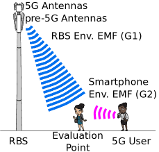
(a) Environmental Exposure

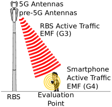
(b) Active Traffic Exposure

Figure 1: Taxonomy of exposure measurements (figure best viewed in colors).

Fig. 1 sketches the main taxonomy of RBS and smartphone exposure measurements over an evaluation point. More in depth, we identify the following groups: $G1$) environmental exposure from 5G RBS, $G2$) environmental exposure from nearby 5G smartphones, $G3$) exposure generated by the 5G RBS when a 5G smartphone is used to inject active traffic in the evaluation point, $G4$) exposure generated by the 5G smartphone in the same condition of $G3$. Intuitively, groups $G1$-$G2$ identify measurements taken without injecting any traffic in the measurement positions, and resulting in general lower exposure levels than groups $G3$-$G4$.

In the following, we initially focus on the works tailored to the RBS side, i.e., covering groups $G1$ and/or $G3$. Then, we focus on the works investigating the active traffic exposure from 5G smartphone (group $G4$). Finally, we consider the works that integrate joint measurement of environmental/active traffic exposure from RBS and active traffic exposure from smartphone (groups $G1$ + $G3$ + $G4$) - although we did not find any previous work tailored to 5G. As a side comment, we intentionally leave apart group $G2$, as the exposure contributions from nearby terminals rapidly decrease to negligible levels when they are not in close proximity to the evaluation point.

2.1 Exposure Measurements from 5G RBS

We initially focus on the works targeting: i) measurement of environmental exposure from 5G RBS (group $G1$) [11, 12, 13, 14, 15] and ii) measurement of active traffic exposure from 5G RBS (group $G3$) [16, 17, 18, 19, 20, 21, 22, 23, 24, 25, 26].

Focusing on $G1$ [11, 12, 13, 14, 15], Chiaraviglio et al. [11] perform a massive evaluation of a 5G RBS covering a town. Betta et al. [12, 13] and Elbasheir et al. [14] collect RBS exposure information through the measurement of the pilot signals. Hausl et al. [15] analyze the received power over the control channels in a 5G network by employing a code-selective measurement methodology.

Focusing on $G3$ [16, 17, 18, 19, 20, 21, 22, 23, 24, 25, 26], Adda et al. [16], Aerts et al. [17], Migliore et al. [18], Bornkessel et al. [19], Schilling et al. [20], Chiaraviglio et al. [21], Liu et al. [22], Heliot et al. [23] share the idea of measuring the exposure from 5G RBSs by forcing traffic with a terminal in the DL direction from the RBS. The works of Aerts et al. [24], Chountala et al. [25] and Wali et al. [26] complement the previous ones by adding the evaluation of 5G RBS exposure when UL traffic is forced with a terminal. In general, such works demonstrate that the exposure from 5G RBS depends on the amount of traffic that is injected towards the measurement location. Moreover, the active traffic contribution from the 5G RBS is generally higher than the environmental one.

Compared to [11, 12, 13, 14, 15, 16, 17, 18, 19, 20, 21, 22, 23, 24, 25, 26], we tackle the 5G EMF measurement from a novel perspective, by including the contribution of the smartphone in the EMF assessments (groups $G1$ + $G3$ + $G4$). Although we exploit some findings/intuitions of the literature (like the idea of forcing DL/UL traffic towards the measurement location), our work presents an innovative measurement framework, called 5G-EA, tailored to the assessment of both smartphone and RBS EMF.

2.2 Exposure Measurement from 5G UE

We focus hereafter on the literature addressing active traffic exposure measurements from 5G UE (group $G4$) [27, 28, 29, 30, 31, 32]. Xu et al. [27] perform measurements of 5G UE power density in a semi-anechoic chamber. Nedelcu et al. [28] analyze the UL contribution from 5G UE in terms of radiated power. Joshi et al. [29] and Lee et al. [30] analyze 5G UE output power levels that are collected from measurements in commercial networks. Deaconescu et al. [31] and Miclaus et al. [32] collect EMF measurement from a 5G UE in an indoor controlled environment, with and without generating UL/DL traffic. Overall, such works indicate that the exposure from 5G smartphones is non-negligible, and that a huge variation in the exposure levels can be observed. In contrast to [27, 28, 29, 30, 31, 32], in this work we go two steps further by: i) integrating the exposure from 5G RBS and ii) performing exposure assessments of groups $G1$ + $G3$ + $G4$ both in indoor controlled environments and into the wild, i.e., several outdoor locations covered by a commercial 5G RBS.

2.3 Joint Measurement of Smartphone and RBS Exposure

The last category relevant to our study is focused on the joint assessment of smartphone and RBS exposure. In this case, we did not find any work covering groups $G1$ + $G3$ + $G4$ in the 5G domain. Focusing instead on pre-5G technologies, the most relevant work to ours is the one of Schilling et al. [10], in which the authors propose a method based on EMF measurements to evaluate the combined exposure from both smartphone and RBS in 4G deployments. Interestingly, a strong reduction in the UL transmission power is observed when the link conditions are improved. Moreover, the total exposure in a macro cell scenario is dominated by the smartphone contribution. Eventually, the authors advocate the need for a balance between RBS and smartphone exposure.

In line with [10], our work is also focused on the joint assessment of smartphone and RBS exposure. However, differently from [10], we focus on a novel domain: the 5G exposure assessment of groups $G1$ + $G3$ + $G4$, which requires a different exposure framework than the one used by [10] for the 4G evaluations. In addition, 5G smartphones currently employ a dual 4G/5G connectivity to support the data transfers. Therefore, our innovative framework evaluates the exposure over both 4G and 5G bands. This last aspects further complicates the exposure assessment compared to [10], since multiple 4G/5G carriers are dynamically used for the data transfer.

3 5G Implementation Aspects Relevant to EMF Monitoring

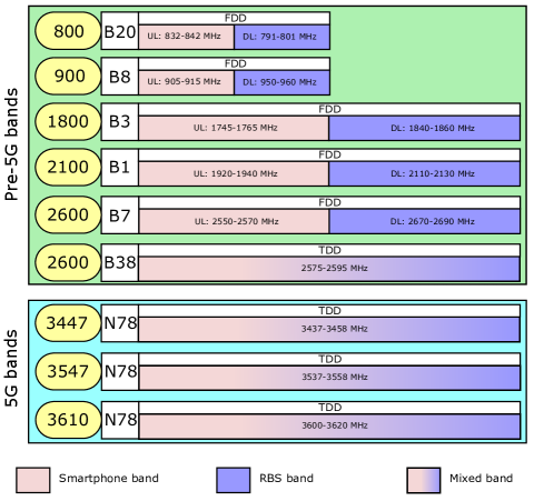
Figure 2: Pre-5G and 5G bands in use by the W3 mobile operator.

In this section, we provide a brief overview of the key 5G implementation aspects that have an influence the design of our EMF assessments, with a focus on the Italian country.

Spectrum Fragmentation. 5G encompasses a wide set of spectrum portions, including frequencies lower than 1 GHz, frequencies between 1 and 6 GHz - a.k.a. the mid-band - and close-to-mm-Wave frequencies at around 26-27 GHz. The most widespread option to provide 5G mobile service in Italy is the mid-band, thanks to the fact that the adopted frequencies can guarantee the mixture of coverage and capacity that is required during the current 5G early-adoption phase.

The mid-band spectrum, spanning over 3.4-3.8 GHz is rather a crowded space. Historically, the 3.4-3.6 GHz portion of the spectrum was allocated to Fixed Wireless Access (FWA) operators [33], which provided access to household customers over legacy technologies (pre-5G). The 3.6-3.8 GHz portion was instead allocated with the purpose of providing 5G service for mobile operators, with licensed spectrum blocks including both 80 MHz and 20 MHz portions [34]. Clearly, the operators that were licensed 20 MHz of 5G mid-band spectrum (like W3) could not support the same level of service as the one provided by providers operating on wider bandwidth, e.g., 80 MHz. To overcome this issue, W3 has recently signed an agreement with the FWA operator Fastweb to lease some portions of the 3.4-3.6 GHz spectrum for the 5G mobile service [35]. Despite the total allocation of licensed and leased bandwidth is non-negligible (typically equal to 60 MHz for W3), the spectrum blocks for delivering 5G in the mid-band are not contiguous. Up to this point, a natural question is: How do such spectrum allocations affect the considered measurements? The answer is that, for some operators (like W3), the 5G EMF monitoring (even focusing solely on the mid-band) has to be done over multiple not-contiguous spectrum portions. Such feature generally complicates the EMF measurement procedure, as it is necessarly (in principle) to iterate over the different 5G bands in use by the same operator to evaluate the total 5G exposure.

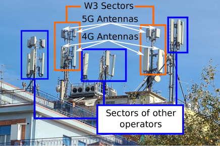
Figure 3: Roof-top installation of W3 operator encompassing multiple sectors and distinct panels for 4G and 5G technologies.

Interviewing of 5G and 4G networks. At the time of preparing this work, the Non Stand Alone (NSA) option, in which the 5G radio access network is supported by a 4G core, is still the most widespread way to implement 5G networks in the country. Compared to a full Stand Alone (SA) deployment, NSA requires a strong dependability of the 5G service with respect to the 4G network. In particular, a 5G connection is always provided in parallel to a 4G one, which acts as the anchor for the dual 4G/5G connectivity [36]. Therefore, our EMF assessments have to include the monitoring of the 4G bands that are used in parallel to the 5G ones, as the injected traffic is (likely) flowing over both 4G and 5G channels. To further complicate such feature, Fig. 2 reports the band allocations of W3 over pre-5G and 5G technologies (valid for the the city of Rome). Astonishingly, the number of possible bands that can be used by 4G is huge, as all the spectrum portions licensed to W3 over 800-2600 MHz frequencies can be potentially used for 4G services.

Dynamicity of carrier aggregation. Another key implementation aspect that strongly affects the EMF monitoring is the (possible) carrier aggregation across multiple 4G bands, which are used in parallel to the 5G ones. As reported in relevant 3GPP standards [37], there are plenty of possible carrier aggregation combinations, ranging from sets composed of 1-2 bands up to ones including several pre-5G spectrum portions in use by the operator. The selected combination of aggregated carriers for a given connection is a local decision, which depends on many features (like the propagation conditions reported by the smartphone) that are monitored by the serving RBS. Consequently, the adopted set of carriers cannot be determined a priori and it depends on the measurement location. The dynamicity in the carrier aggregation has to be taken into account in our measurement procedures, in order to limit the exposure assessment only on those bands that are used for the transfer of the injected traffic.

Time Division Duplexing. Fig. 2 details the assignment of frequencies for the UL and DL directions. In different spectrum portions (B20, B8, B3, B1 and B7), the Frequency Division Duplexing (FDD) rigidly separates the UL frequencies with respect the DL ones. On the other hand, the B38 spectrum of 4G and all the 5G portions in use by W3 (covering the N78 band) are employing the Time Division Duplexing (TDD), which adopts multiplexing of both UL and DL over the same frequencies. Intuitively, TDD complicates the dissection of smartphone vs. RBS exposure contributions, as both time-frequency domains have to be jointly analyzed to distinguish the DL from the RBS with respect to the UL from the smartphone.

RBS co-location. Fig. 3 shows a typical roof-top RBS installation, which includes multiple 5G and 4G sectors of W3 operator, as well as radio equipment of other operators that are co-located on the same site. Since our goal is to consider the impact of smartphone and RBS exposure for a given connection, we need to distinguish the EMF contribution of the considered operator with respect to the co-located ones that serve the same area (i.e., the sectors of other operators in the figure).

4 5G EMF Measurement Requirements

TABLE I: 5G Features & Goals vs. EMF Measurement Requirements.

Feature/Goal		Requirement
FG1	Operator and Technology Impact	Narrow-band frequency-selective measurements	R1
FG2	5G (and 4G) TDD	Dissection of smartphone vs. RBS exposure	R2
FG3	45/5G Dual Connectivity	Multiple monitoring over 4G and 5G technologies	R3
FG4	Spectrum Fragmentation	Detection & iteration
FG5	Dynamic carrier aggregation	over the adopted set of carriers	R4
FG6	Impact of traffic	Forcing smartphone traffic in the UL/DL directions	R5
FG7	Impact of propagation	Selection of representative measurement locations	R6

We analyze hereafter the measurement requirements that are instrumental for the definition of the EMF monitoring framework, starting from the goals of our work in Sec. 1 and the implementation features detailed in Sec. 3. To this aim, Tab. I highlights the transition from 5G features and goals (FG1-FG7) into concrete EMF measurement requirements (R1-R6).

More in depth, the need of distinguishing the 5G exposure contribution w.r.t. other technologies and/or other operators (FG1) impose to adopt an approach based on narrow-band frequency-selective measurements (R1). This is a first and important requirement, as narrow-band measurements can be performed only by adopting more complex instrumentation tools and procedures than the ones used for wide-band approaches. Secondly, the adoption of TDD in 5G bands (FG2) requires to define a measurement methodology able to dissect the smartphone exposure contribution vs. the RBS one, which, obviously, cannot be based on frequency separation (R2). Third, the dual connectivity between 4G/5G (FG3) requires to perform both 4G and 5G exposure assessments (R3). Fourth, the adoption of non-contiguous 5G portions in a fragmented spectrum (FG4), as well as the dynamic carrier aggregation feature (FG5), suggest that the EMF measurements should be done only on the combination of 4G/5G carriers in use by a given connection. Therefore, rather than iterating over the whole set of spectrum portions assigned to the operator - an operation that would result in a waste of time and resources - a mechanism able to detect the carriers used for a given data transfer should be designed (R4). Such feature should be complemented by an EMF measurement procedure (possibly automated) able to iterate over the selected set of carriers and measure the exposure on each carrier (R4). Fifth, the impact of traffic (FG6) has to be evaluated with a procedure able to force the traffic in UL/DL directions (R5). Finally, the impact of propagation (FG7) can be solely assessed by selecting a representative set of measurement locations (R6), subject to meaningful propagation conditions (e.g., LOS/NLOS, RBS proximity/distance). It is also clear that FG6 and FG7 inherently require that the adopted measurement chain should be easily portable over the territory, as several measurements in different locations should be performed in order to retrieve a meaningful set of results.

5 5G-EA Framework Description

We divide the presentation of the 5G-EA framework into the following steps: i) measured exposure metrics, ii) adopted tools and HardWare (HW) chains, iii) description of measurement algorithm, and iv) implementation details.

5.1 Measured Exposure Metrics

In principle, any exposure assessment strongly depends on the target metrics that need to be measured. In particular, the classical taxonomy defines Specific Absorption Rate (SAR)/absorbed power density for UE assessments vs. electric field/plane-wave power density for RBS evaluation [4]. The SAR and absorbed power density metrics are useful when the measurement target is the near-field assessment, in which the radiating source is (almost) attached to the body (e.g., an UE close to the ear during a phone call). Despite such metrics are still relevant for today equipment (and for UE SAR-based limits), we point out that the typical smartphone user makes phone calls with the equipment attached to the ear only to a limited extent. In fact, recent statistics [38] reveal that smartphones are mainly used for downloading/uploading data traffic, with the UE hold at a non negligible distance from the head/chest in order to read/produce content on the screen. Since our goal is to evaluate the exposure in such conditions - which represent a typical 5G scenario - in this work we always impose a minimum distance between the UE generating traffic and the evaluation point of our measurement.

TABLE II: Frequencies, wavelengths, Fraunhofer regions and far field distances for the W3 bands with smartphone antenna length $L_{\text{A}}=0.08$ [m].

Frequency $f$	Wavelength $\lambda_{f}$	Fraunhofer Region $\frac{2L_{\text{A}}^{2}}{\lambda_{f}}$	Far-field distance $D^{\text{FF}}_{f}$
800 [Mhz]	0.37 [m]	0.03 [m]	$>$0.37 [m]
900 [Mhz]	0.33 [m]	0.04 [m]	$>$0.33 [m]
1800 [Mhz]	0.16 [m]	0.08 [m]	$>$0.16 [m]
2100 [Mhz]	0.14 [m]	0.09 [m]	$>$0.14 [m]
2600 [Mhz]	0.12 [m]	0.11 [m]	$>$0.12 [m]
3447 [Mhz]	0.09 [m]	0.15 [m]	$>$0.15 [m]
3547 [Mhz]	0.08 [m]	0.15 [m]	$>$0.15 [m]
3610 [Mhz]	0.08 [m]	0.15 [m]	$>$0.15 [m]

Apart from better matching the actual smartphone usage, the introduction of a minimum distance between the UE and the measurement point may allow operating in the far-field region from the UE, which is formally defined as:

$$D^{\text{FF}}_{f}>\max\left(\lambda_{f},L_{\text{A}},\frac{2L_{\text{A}}^{2}}{\lambda_{f}}\right)$$ (1)

where $\lambda_{f}$ is the wavelength of frequency $f$, $L_{\text{A}}$ is the length of the radiating antenna, while the term $\frac{2L_{\text{A}}^{2}}{\lambda_{f}}$ represents the limit of the Fraunhofer region. To give an example, Tab. II reports the values of $\lambda_{f}$ and $D^{\text{FF}}_{f}$ for the bandwidth allocation of W3 and a smartphone antenna length $L_{\text{A}}$ equal to 0.08 [m]. As expected, the observed far-field distances $D^{\text{FF}}_{f}$ strongly depend on the considered frequencies, but, however, we can note that the minimum $D^{\text{FF}}_{f}$ is lower than $0.2$ [m] for 4G frequencies above or equal 1800 [MHz] and for all 5G frequencies.

By imposing the distance $D^{\text{FF}}_{f}$ from the UE, we are able to operate in far-field, a condition that is also generally experienced when considering the RBS as the source of radiation. In this way, an homogeneous set of metrics (e.g., electric field and/or plane-wave power density) can be used to measure both UE and RBS exposure. This is in turn beneficial for adopting the same measurement equipment when assessing the UE/RBS exposure, as detailed in the following subsection.

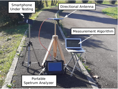
(a) Exposure Assessment and Traffic Generation Chains (UE side)

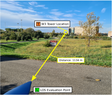
(b) Isolation of RBS contribution for a measurement point in LOS conditions.

Figure 4: Views of the equipment tools in a given measurement location.

5.2 Tools and HW Chains

We describe hereafter the equipment tools, which are also sketched in Fig. 4(a). Focusing on the exposure assessment chain, we employ the following HW ($E1$-$E5$):

1. Hand-held Spectrum ANalyzer (SAN) Anritsu MS2090A with maximum frequency range equal to 32 [GHz] with 110 [Mhz] of maximum bandwidth analysis, equipped with one battery plus another one of backup;

2. Directive antenna Aaronia 6080, with frequency range 680 [MHz]-8 [GHz], maximum gain equal to 6 [dBi], nominal impedance of 50 [Ohm];

3. Coaxial cable Anritsu flexible RF 1 [m] Cable K(f)-K(m) DC-40 [GHz], connecting the SAN to the directive antenna;

4. Laptop MacBook Air with Intel Core i5 1.3 [GHz] CPU, 4 [GB] of RAM, 256 [GB] of memory, equipped with Matlab R2017b and RSVisa 5.12.1 driver;

5. Ethernet cable of 1 [m] length, Cat.5E, verified TIA-EIA-568-C.2, connecting the laptop to the SAN.

Focusing on $E1$, the SAN allows implementing narrow-band measurements, and thus matching requirement $R1$. Focusing then on $E2$, the directionality of the adopted antenna allows spatially separating the contribution of the UE and the one of the RBS. As shown in Fig. 4(b), the antenna is oriented towards the considered source. In this way, the contribution of other sources, e.g., a UE placed behind the measurement antenna, is not sensed. By selectively pointing the directive antenna towards the UE or the RBS, we can isolate their respective contributions, and thus matching requirement $R2$, even when the monitoring is performed over TDD bands. In addition, the short coaxial cable of $E3$ guarantees almost negligible signal degradation between the directive antenna and the SAN - a feature that is instrumental for measuring the relatively low environmental exposure values of 5G. The SAN is then connected to the $E4$ laptop via the dedicated $E5$ cable. The core of our framework is a custom measurement algorithm written in Matlab and running on $E4$. The algorithm allows remotely programming the SAN to perform multiple monitoring of 4G and 5G bands (requirement $R3$), as well as to implement the automatic detection and iteration over the adopted set of carriers (requirement $R4$).

Focusing then on the traffic generation chain, we adopt the following tools:

1. Samsung S20+ 5G smartphone, equipped with Android 11 (1st May 2021) and Magic Iperf v.1.0 App client.

2. Dell Poweredge R230 server, equipped with 4 cores Intel Xeon E3-1230, 64 GB of RAM, Ubuntu 18.04.1 OS and Iperf v.3.1.3.

More concretely, $T2$ is installed at the University building, and made accessible through a public Internet Protocol (IP) address. In addition, the Iperf program is used to generate synthetic traffic between $T1$ and $T2$ (either in the DL or UL direction). In this way, we accomplish requirement R5.

Fig. 4(a) shows the measurement setup in a given location. Both smartphone and SAN are placed on tripods above around 1 [m] from ground, in order to mimic exposure evaluations representative of users. The required setup does not involve any electricity plug. This fact, coupled also with the overall small size of $E1$-$E5$ and $T1$ (as shown in Fig.4(a)), as well as the availability of a second backup battery for the SAN, allows easily repeating the measurements in different locations of the territory, and thus matching requirement $R6$.

5.3 Algorithm Description

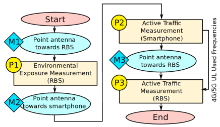
Figure 5: High level steps of the measurement algorithm implemented in 5G-EA.

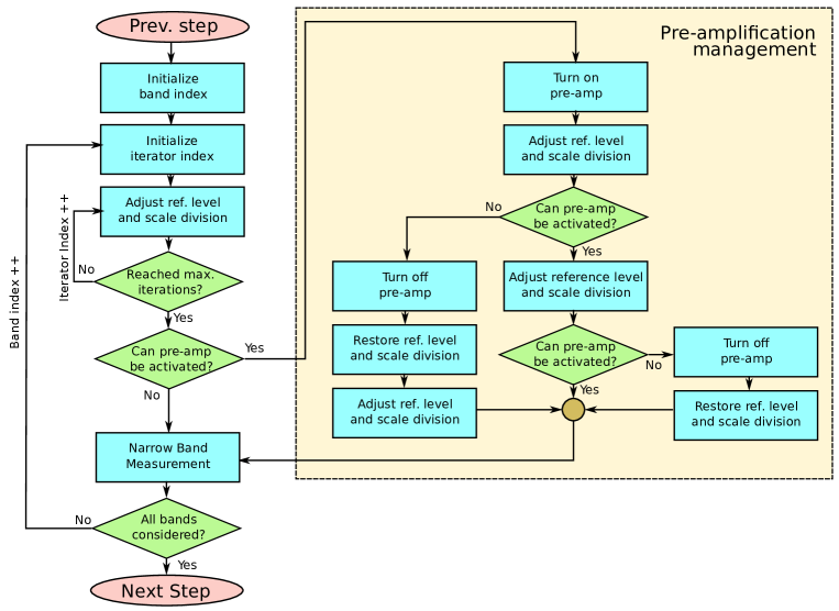
Figure 6: Steps to perform $P1$ (RBS environmental exposure).

Fig. 5 provides a high level description of the measurement algorithm implemented in the 5G-EA framework. In more detail, we apply a divide-et-impera approach to split the complex measurement procedure into the following sub-problems: i) evaluation of RBS environmental exposure (step $P1$), ii) evaluation of active traffic exposure from the smartphone (step $P2$), iii) evaluation of active traffic exposure from the RBS (step $P3$). In addition, the algorithm is complemented by three manual orientations $M1$-$M3$ of the directive antenna, which are instrumental to correctly separate RBS vs. smartphone contributions. More concretely, the directive antenna is pointed towards the RBS before starting $P1$ ($M1$ block of Fig. 5), then it is pointed towards the smartphone before running $P2$ ($M2$ block), and finally it is pointed again towards the RBS before executing $P3$ ($M3$ block).

Intuitively, all the considered bands in use by the operator (TDD and DL FDD) are swept during the environmental exposure assessment of $P1$. Then, the goal of $P2$ is to restrict the set of monitored bands only on those ones in use by the current active traffic connection - which is kept alive from $P2$ to $P3$. In this way, the monitoring during $P3$ is done on the same traffic conditions that are experienced in $P2$.

In the following, we describe in more details steps $P1$-$P3$.

Algorithm 1 Pseudo-Code of the adjust_ref_level_scale_div routine of $P1$

Input: set of SAN_settings, current frequency start curr_f_min, current frequency stop curr_f_max, safety margin for the ref. level safety_margin, maximum time (in s) for searching the maximum level max_time_search, pre-amplifier state pre_amp_state, minimum level matrix min_l, number of y ticks on the screen y_ticks
Output: ref_level, scale_div

1:set_SAN(SAN_settings);

2:max_l=-200;

3:for i=1:max_time_search do

4:    max_l=max_lev_search(max_l,curr_f_min,curr_f_max);

5:    sleep(1);

6:end for

7:ref_level=ceil(max_l)+safety_margin;

8:set_SAN(ref_level);

9:scale_div=abs(ref_level-min_l(curr_f_min,pre_amp_state))/ y_ticks;

10:set_SAN(scale_div);

5.3.1 P1 - Environmental RBS EMF

Fig. 6 shows the high level flowchart of $P1$. Initially, the set of bands to be monitored are selected, based on the operator that is under consideration. For example, in the case of W3 operator all TDD and DL FDD bands shown in Fig. 2 are considered for the environmental assessment of RBS exposure. The algorithm then iterates over the set of bands. For each considered band, an automatic procedure to adjust reference level and scale division of the observed signal is implemented. Intuitively, the reference level is the upper limit of the y axis in a spectrum plot (where the x axis is the set of monitored frequencies), while the scale division allows tuning the unit of the y ticks and consequently the lower limit on the y axis. By jointly optimizing the reference level and the scale division, we can achieve a double goal: i) the signal that is being monitored can be qualitatively checked on the screen of the SAN, ii) the measurement resolution is tuned to the actual signal that is observed, and thus the impact of (possible) measurement uncertainties is limited.

More specifically, the adjustment of the reference level and scale division reported in the flow chart of Fig. 6 is sketched in the adjust_ref_level_scale_div routine of Alg. 1. This function requires as input a set of basic SAN settings (whose values are going to be presented in detail in Sec. 6.2.2), the starting and ending frequency for the considered band (curr_f_min and curr_f_max), the safety_margin parameter that is used when setting the reference level, the max_time_search parameter to govern the maximum time for searching the maximum reference level, the pre_amp_state boolean variable storing the state of the SAN pre-amplifier (active or inactive), the min_l matrix including the values of the minimum sensed levels (which depend on the adopted frequency and the pre-amplifier state) and the y_ticks parameter representing the number of y ticks on the SAN screen.

The routine then proceeds as follows. The basic SAN settings are implemented in line 1, which include e.g., the detector type, the measured unit, and the trace detector. The maximum signal level max_l is initialized to a very low value in line 2. Then, a live searching of max_l is iteratively performed in lines 3-6, up to the maximum time max_time_search. At the end of this step, the maximum recorded signal level is stored in max_l. The reference level ref_level is then set by adding to max_l the safety margin in line 7. In line 8, the resulting reference level is applied. In addition, the exact scale division, in order to entirely show the dynamics of the signal between ref_level and min_l, is computed in line 9 and then applied to the SAN in line 10.

The execution of Alg. 1 is then iterated up to a maximum number (iterator index in the flowchart of Fig. 6), in order to improve the setting of reference level and scale division. In the following step, a check on the pre-amplification is performed. If the current reference level is lower than a pre-amplification threshold, the signal can be pre-amplified by the SAN (right part of Fig. 6). Such feature is particularly useful for the environmental assessment of 5G signals, which are normally very low and close to the equipment noise level, due to a relatively low usage of 5G on such early phase of adoption. After turning on the pre-amplifier, the adjust_ref_level_scale_div routine is called again, in order to adjust the amplified signal levels. However, this procedure may increase the reference level again above the maximum one allowed by the pre-amplifier. Consequently, a check on the pre-amplification threshold is done again. In case pre-amplification can be kept turned on, a further adjustment of reference level and scale division is done - and a further check on the pre-amplification is performed. In case pre-amplification is not supported, the pre-amplification is turned off, the reference level and scale division are reverted back to the last values before pre-amplification, and (eventually) a further call of the adjust_ref_level_scale_div routine is run.

Algorithm 2 Pseudo-Code of the nar_band_meas routine of $P1$, $P2$ and $P3$

Input: set of basic SAN_settings, current frequency start curr_f_min, current frequency stop curr_f_max, number of samples n_samples, inter sample time (in s) int_sample_time
Output: Array of exposure values curr_exp in dBm/m² ($P1$) or V/m ($P2$ and $P3$)

1:set_SAN(SAN_settings);

2:for i=1:n_samples do

3:    curr_exp(i)=get_SA(curr_f_min,curr_f_max);

4:    sleep(int_sample_time);

5:end for

After setting reference level and scale division (and eventual activation of pre-amplification), the signal is ready to be measured. To this aim, a narrow band measurement, expanded in Alg. 2, is invoked. The function takes as input a set of basic SAN settings, the current frequency start curr_f_min and frequency stop curr_f_max, the number of sampled channel power measurements n_samples, and the inter-sample time int_sample_time. The routine then produces as output an array of exposure values curr_exp. The logic of the procedure is very simple: after setting the SAN parameters, a channel power computation function is iteratively invoked on the SAN. When all the samples are recorded, the algorithm returns the array of exposure measurements curr_exp. At the end of $P1$, the RBS environmental exposure is measured for the set of bands in use by the operator.

5.3.2 P2 - Active Traffic Smartphone EMF

The goal of the second part of the algorithm is to perform the assessment of the exposure generated by the smartphone upon active traffic generation. To this aim, the dual 4G/5G connectivity and carrier aggregation features suggest that multiple bands (unknown a-priori) can be used in parallel for the data transfer. On the other hand, measuring the exposure on the entire set of bands in use by the operator may result in a waste of resources, in terms of: i) overly increase of time to perform the assessment, ii) waste of consumption of the SAN battery (which is a precious resource) and iii) excessive traffic consumption on the smartphone (which may be critical for limited data traffic plans). To face such issues altogether, $P2$ adopts the following intuition. First, the TDD and UL FDD bands in use by the data transfer are detected. Then, the exposure assessment is done only on the selected subset of spectrum portions currently in use.

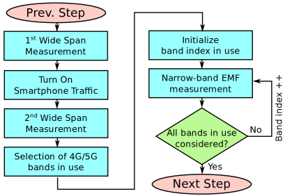
Figure 7: Steps to perform $P2$ (active traffic smartphone exposure).

To this aim, Fig. 7 sketches the main operations performed during $P2$. Initially, a wide span assessment is done, in order to detect the peak(s) of the sensed signals on a very large range of frequencies (including all the ones in use by the operator under investigation). The goal of this scan is not to measure exposure, but rather to get a quick indication on the frequencies that carry most of signal power before injecting any traffic. In the following step, the active traffic is generated towards the smartphone, by executing the Iperf program. Then, a second wide span assessment is done. The detection of the subset of 4G/5G bands in use for the data transfer is done by comparing the peaks recorded during the first scan vs. the ones observed on the second one.

Algorithm 3 Pseudo-Code of the sel_band_use routine of P2

Input: array of EMF values from 1st span emf_array_1st_span, array of EMF values from 2nd span emf_array_2nd_span, array of frequency values freq_array, threshold increase parameter thre_inc
Output: array of selected bands sel_band_array

1:sel_band_array=initialize();

2:for f=1:size(freq_array) do

3:    if incr_percent(emf_array_2nd_span_rev(f), emf_array_1st_span(f)) $>$ thre_incr then

4:         band_index=find_b_index(f);

5:         sel_band_array(band_index)=1;

6:         if fdd_array(band_index)==1 then

7:             band_index_fdd=find_b_index(f,FDD);

8:             sel_band_array(band_index_fdd)=1;

9:         end if

10:    end if

11:end for

The detection of the 4G/5G bands is expanded in Alg. 3. The routine takes as input the emf_array_1st_span array of EMF values (indexed by frequency) that were sensed during the first span, the emf_array_2nd_span array of EMF values that were sensed during the second span, and a threshold increase parameter thre_inc (in %) to activate the detection. The algorithm then produces as output the subset of bands sel_band_array that are detected for the current data transfer. The logic of the function is quite simple: for each considered frequency, the sample in emf_array_2nd_span is compared against the corresponding one emf_array_1st_span, by computing the percentage variation of EMF. If such variation is greater than the thre_inc parameter, the band is included in the list of spectrum portions that are monitored for the current data transfer. The intuition here is in fact to exploit the increase of EMF as a result of the usage of specific bands in the UL. In case the current selected band employs FDD, then the corresponding one in the DL is also included in the list of selected ones. For example, let us assume that the 1745-1765 [MHz] band of Fig. 2 is detected in the UL. This portion of the spectrum belongs to the B3 FDD band, which also includes the 1840-1860 [MHz] band for the DL. This second portion will be likely used when evaluating the active traffic from the RBS, and therefore it is included in the list of bands to be monitored - when considering RBS active traffic exposure. At the end of the algorithm the array sel_band_array stores the list of band indexes in use for the current data transfer.

Coming back to the flowchart of Fig. 7, the blocks on the right details the steps for the EMF assessment on the selected set of bands. In particular, the initial band is selected - the index in sel_band_array with lowest frequency and belonging to UL. Then, the narrow-band EMF measurement on the selected band is performed. The logic is in common with the exposure measurement of $P1$, and sketched in Alg. 2. In particular, the main differences rely on a different set of basic SAN settings and on a different measurement metric (in terms of V/m). Once the measurement has been completed for the current band, $P2$ passes to the next one, until all the TDD and UL FDD bands in sel_band_array are considered (band index in Fig. 7). At the end of $P2$, a set of exposure arrays, one for each considered band, is available.

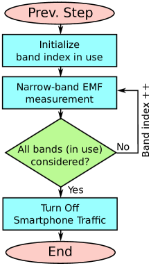
Figure 8: Steps to perform $P3$ (active traffic RBS exposure).

5.3.3 P3 - Active Traffic RBS EMF

The last part of our measurement technique involves the assessment of RBS exposure while keeping active the current data transfer. Fig. 8 highlights the main blocks that realize this functionality. The logic is very similar to the smartphone assessment, except for the following differences: i) the evaluation include TDD and FDD DL bands (with the directive antenna pointed towards the RBS), ii) the smartphone traffic is turned off after completing the scan over the considered band. Similarly to $P2$, a set of exposure arrays is available at the end of the procedure.

5.4 Implementation Details

We implement $P1$-$P2$-$P3$ parts of 5G-EA framework as a set of scripts written in Matlab - except from the traffic generation, which is governed by the Iperf program running on the smartphone and dedicated server. An unique aspect of our framework is the implementation of the measurement algorithm in software, on a general purpose machine that controls the SAN. This is another innovation brought by our work, which opens the way for possible future investigation in the softwarization of EMF assessments.

More technically, the high level functionalities reported in $P1$-$P2$-$P3$ are translated into a set of basic operations, coded as low-level Standard Commands for Programmable Instruments (SCPI) and transfered from/to the SAN through a Transmission Control Protocol (TCP) connection. The output of the SAN (e.g., the array including the exposure values) are then sent back over the same connection in SCPI format. In this way, the process is completely automated and the the post-analysis of the obtained data can be done directly in Matlab - in the same script running the measurement algorithm.

6 Results

We present our outcomes through the following steps: i) description of evaluation scenarios, ii) parameter settings of 5G-EA framework, iii) exposure assessments.

6.1 Evaluation Scenarios

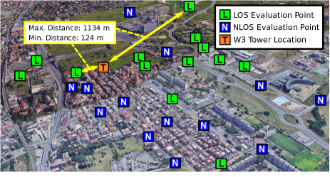
Figure 9: Positioning of W3 tower and outdoor LOS (L green square) and NLOS (N blue square) measurement locations (map source: Google Maps) - figure best viewed in colors.

We consider a set of measurement points in the coverage area of the W3 roof-top installation shown in Fig. 3, with the frequency assignment reported in Fig. 2. The installation is located in the area close the University of Rome Tor Vergata in Rome (Italy). More concretely, we perform our experiments in both outdoor and indoor locations, due to the following reasons. First, we aim at massively performing measurements under different propagation conditions, which are obviously influenced by terrain parameters like the distance from the RBS, the level of urbanization around the measurement point and the presence of buildings/obstacles on the path towards the RBS. Second, we exploit the indoor locations to perform detailed and in-depth measurements, with the goal of corroborating the results from the outdoor locations with tests covering e.g., sensitivity analysis of the exposure vs. variation key parameters, such as throughtput, distance from the smartphone, and smartphone orientation.

Focusing on the outdoor tests, Fig. 9 reports a 3D map of the measurement locations. In total, 26 measurement locations are selected for the tests, based on the following criteria: i) spreading the tests over the territory around the W3 tower, and ii) finding locations that are suitable for placing the instruments (e..g., avoid private streets, locations in close proximity to each other, etc.). The 3D distance of each measurement location from the RBS varies between a minimum of 124 [m] up to a maximum of 1134 [m], in order to capture a wide set of exposure conditions. In addition, the measurement points are placed in the coverage area of each W3 sector shown in Fig. 3, in order to further strengthen our analysis. We refer the reader to Appendix A, which provides detailed information about: i) radio configuration of the W3 installation under consideration, ii) other RBSs in the surroundings of the considered area, iii) taxonomy of outoor locations, iv) measurement time.

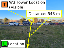
(a) LOS Location - Engineering Parking

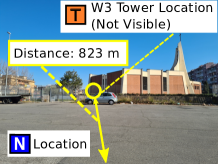
(b) NLOS Location - Church Square

Figure 10: Example of LOS and NLOS outdoor measurement locations.

To give more insights, Fig. 10 reports two representative examples of outdoor measurement points. When considering LOS locations (Fig. 10(a)), the RBS is visible from the measurement point. On the contrary, the installation is not visible in NLOS locations (Fig. 10(b)). In both cases, the directive antenna is pointed towards the RBS location during operations $M1$ and $M3$.

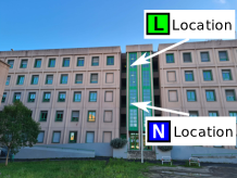
(a) Positioning of LOS and NLOS indoor locations

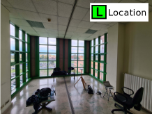
(b) View of LOS indoor location

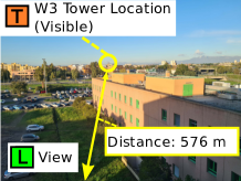
(c) Window view from LOS location

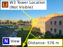
(d) Window view from NLOS location

Figure 11: LOS and NLOS indoor measurement locations.

Focusing then on the indoor tests, we consider two locations at the Engineering building of the University, shown in Fig. 11(a). In particular, we consider a LOS location at the fourth floor and a NLOS one at the second one. The room hosting the LOS measurements is shown in Fig. 11(b). In addition, the environment hosting the NLOS tests is identical to the LOS one (not shown due to the lack of space). Interestingly, the walls are made of thin concrete pillars and big glasses that are mounted on small metallic frames. This structure provides in general good penetration of outdoor mobile signals inside the building. The window view from both locations is shown in Fig. 11(c)-Fig. 11(d). Focusing on the LOS environment, the path towards the RBS is free from obstacles and the distance is within the RBS coverage area. Focusing instead on the NLOS location, the distance from the RBS is identical to the LOS one, but, obviously, the RBS sight is obstructed by a building, which forces the signal to follow a NLOS path.

6.2 Parameters Settings

We provide herefater the settings of the main parameters of 5G-EA framework. In particular, we shed light on the measurement antenna positioning and the algorithm parameters in $P1$, $P2$, and $P3$, respectively. We refer the reader to Appendix B for more insights about calibration and uncertainty aspects of the measurement chain.

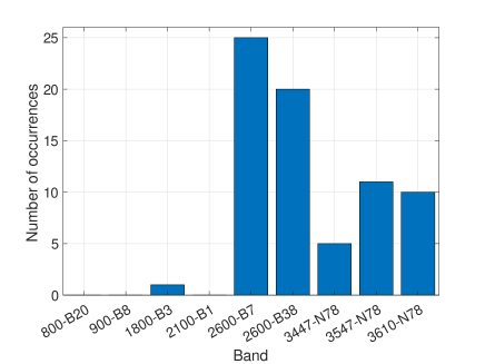
Figure 12: Occurrence of bands used for the 4G/5G data transfers in the considered scenarios

6.2.1 Measurement Antenna Placement

5G-EA requires a careful orientation and positioning of the measurement antenna, in order to properly dissect RBS vs. smartphone exposure. Focusing on $M1$ and $M3$, the antenna is simply pointed towards the RBS location. Focusing on $M2$, the antenna is pointed towards the smartphone. As already shown in Tab. II, the far-field distance $D_{f}^{\text{FF}}$ has to be enforced in our experiments, in order to avoid near-field effects. On the other hand, the distance should mimic the actual exposure conditions to the head/chest that is experienced by a typical user. Therefore, there is trade-off between the (small) distance for a meaningful assessment and the (relatively large) distance that has to be enforced to preserve far-field conditions. In this work, we have found that a good compromise among such competing goals can be achieved by setting a distance from the smartphone equal to 0.25 [m]. Although this number may apparently violate the far-field conditions for the 800 [MHz] and 900 [MHz] bands (as shown in Tab. II), in practice we have found that such bands are not used for 4G data transfers.

To corroborate the previous outcome, Fig. 12 reports the occurrence of bands that are used for the data transfers in the outdoor locations of our experiments. Interestingly, most of transfers employ 4G bands at around 2600 [MHz], while the 1800 [MHz] band is seldom used. On the other hand, the 800 [MHz] and 900 [MHz] bands are not used by the data transfers. Eventually, all the three 5G bands at 3.4-3.6 [GHz] are almost equally adopted. In this way, the minimum frequency used for the exposure assessment can be assumed to be the 1800 [MHz], band. Therefore, the distance of 0.25 [m] is sufficiently large to provide far-field conditions.

TABLE III: Parameters of adjust_ref_level_scale_div routine ($P1$).

	Parameter	Value/Setting
	Unit	dBm/m2
	Attenuation	Auto
	Resolution Bandwidth	Auto
	Video Bandwidth	Auto
	Number of sweep points	Auto
	Trace Detector	Root Mean Square (RMS)
	Type Detector	Rolling Max
	Initial Reference Level	65 dBm/m2
SAN_settings	Initial Scale/Div	15
	curr_f_min	Fig. 2 (FDD DL, TDD)
	curr_f_max
	pre_amp_state	Fig. 6
	min_l	Tab. IV
	pre_amp_thre	-48.77 dBm/m2
	safety_margin	10 dBm/m2
	max_time_search	5 s
Param. Settings	y_ticks	10

TABLE IV: min_l values as a function of frequency and pre-amplifier state.

	min_l
curr_f_min	pre_amp_state=0 (inactive)	pre_amp_state=1 (active)
791, 832, 950, 905 [MHz]	-100 [dBm/m2]	-115 [dBm/m2]
1840, 1745, 2110, 1920 [MHz]	-95 [dBm/m2]	-107 [dBm/m2]
2670, 2550, 2570 [MHz]	-90 [dBm/m2]	-103 [dBm/m2]
3437, 3537, 3600 [MHz]	-85 [dBm/m2]	-97 [dBm/m2]

6.2.2 $P1$ Parameters

Tab. III reports the parameters of the adjust_ref_level_scale_div function. In more detail, the upper part of the table expands the basic SAN parameters. In particular, we adopt a rolling max type detector, as our goal here is to first sense the maximum signal levels and then adjust accordingly reference level and scale division. Focusing on the other routine parameters (bottom part of the table), the values of curr_f_min and curr_f_max are taken from Fig. 2, by considering the W3 bands over FDD DL and TDD - since the exposure from RBS is the target of $P1$. In addition, the pre-amplifier state (on/off) is governed by the logic reported in Fig. 6. Obviously, the pre-amplifier is inactive when the first call of adjust_ref_level_scale_div is run (left part of Fig. 6). However, in case the pre-amplification management branch is followed (right part of Fig. 6), the pre_amp_state state that is passed to adjust_ref_level_scale_div may be active.

Focusing on the remaining parameters of adjust_ref_level_scale_div, the min_l matrix is reported in Tab. IV. The values reported in the table are retrieved by visualizing the noise level on the SAN in each considered band. Clearly, when the pre-amplifier is turned on, the noise level can be notably reduced (right part of the table). Moreover, the pre_amp_thre threshold, which is used in the decision block of Fig. 6 to compare the reference level and activatate/deactivate the pre-amplification, is set to -48.77 dBm/m² (a setting that depends on the SAN HW and the features of the directive antenna). In addition, the safety_margin parameter is set to 10 [dBm/m²] - an empirical value that was tested to correctly work on all the considered bands. Finally, the maximum time for searching the signal peak over the considered band is set to 5 [s], while the number of y ticks is set to y_ticks=10. In this way, the time required to run a single call of adjust_ref_level_scale_div is at least equal to 5 [s].

TABLE V: SAN and parameter settings for the nar_band_meas routine of $P1$, $P2$ and $P3$.

		Value/Setting
	Parameter
		$P1$	$P2$, $P3$
	Unit	dBm/m2	V/m
	Attenuation	Auto
	Resolution Bandwidth	Auto
	Video Bandwidth	Auto
	Sweep points	Auto
	Trace Detector	Root Mean Square (RMS)
	Type Detector	Rolling Average
	Avg. samples	100
	Reference Level	Set by the logic in Fig. 6	6 V/m
SAN_settings	Scale/Div	Set by the logic in Fig. 6	Automatic
	curr_f_min	Fig. 2 (FDD DL, TDD)	Extracted from
	curr_f_max		sel_band_array
	n_samples	12
Parameters	int_sample_time	0.5 s

Tab. V reports the parameters for the nar_band_meas function. Focusing on the $P1$ settings (central column), the set of SAN_parameters this time includes a rolling average as type detector, as our primary goal during this step is to perform an exposure assessment over the considered signal. This setting is inline with relevant measurement standards in the field (see e.g., [39]). In addition, the number of samples for computing the average is set to 100, in order to consider a meaningful range. Clearly, the reference level and the scale division are updated by the logic implemented in Fig. 6. Focusing then on the remaining parameters, curr_f_min and curr_f_max are set in accordance to the set of W3 bands shown in Fig. 2 (restricted to FDD DL and TDD). Finally, the number of narrow band measurements n_samples is set to 12, while the time between consecutive queries of narrow band measurements is set to 0.5 [s]. In this way, the measurement time for each band is approximately equal to 12 $\times$ 0.5 [s] = 6 [s].

Finally, we shed light on the remaining parameters that appear in Fig. 6. Focusing on the maximum number of iterations for running the adjust_ref_level_scale_div function, we set it to 3 - a value that provides a good balance between overall duration of detection phase and precision in setting reference level and scale division values. Focusing on the number of bands to be monitored, we set it to 9, in accordance to the FDD DL and TDD bands of W3 shown in Fig. 2. With such settings, the required time to run $P1$ is at least equal to (5 [s] $\times$ 3 + 6 [s]) $\times$ 9 = 189 [s]. However, the actual total time for running $P1$ may be higher, due to the following reasons: i) the additional delay that is required when communicating with the SAN and ii) the eventual activation of the power amplifier, which requires further calls of the adjust_ref_level_scale_div routine.

6.2.3 $P2$ Parameters

TABLE VI: SAN settings for wide span measurements $P2$.

Parameter	Value/Setting
Unit	V/m
Attenuation	Auto
Pre-amplifier	Off
Frequency Start	791 MHz
Frequency Stop	3620 MHz
Resolution Bandwidth	Auto
Video Bandwidth	Auto
Sweep Points	Auto
Trace Detector	Root Mean Square (RMS)
Type Detector	Max. Detector
Reference Level	6 V/m
Scale/Div	Automatic

We initially consider the parameters of the wide span measurement blocks reported in Fig. 7, detailed in Tab. VI. More in depth, most of SAN parameters are set to the default values (i.e., automatic setting). Focusing on the remamining parameters, the selected frequencies cover all the ones in use by W3 operator. In addition, the pre-amplifier is powered off, as the exposure from the smartphone may be potentially higher than the maximum supported signal level with pre-amplification turned on - which we remind is a very effective feature to distinguish low signals w.r.t. noise level. Moreover, the reference level is set to a large value (6 [V/m]) in order to detect possible signal peaks. Focusing on the trace detector, a root mean square (RMS) setting is imposed (in line with $P1$). Eventually, the max detector is used, as we remind that the scope of the wide span measurement is to perform a quick scan over the entire frequency range and to detect the signal peaks.

The second block of $P2$ is the activation of the smartphone traffic exposure. Unless otherwise specified, the iperf client is run on the smartphone with the following parameters: i) IP address and port corresponding to the iperf server installed at the University, ii) bandwidth report interval set to 1 [s], iii) number of simultaneous connections per data transfer set to 1, iv) maximum duration of iperf transfer set to 120 [s] - an amount of time sufficiently large to complete the remaining steps in $P2$ and $P3$.

In the following, we focus on the parameters for selecting the 4G/5G bands in use by the data transfer (expanded in the sel_band_use routine of Tab. 3). Obviously, the array of EMF measurements are set by the first and second wide span assessment. The array of frequency values freq_array includes all the frequencies in use by W3 operator. Finally, the treshold increase parameter thre_inc is set to 30% - a value that guarantees a good balance between (artificial) increase of EMF due to injection of traffic from the smartphone and (natural) variation of exposure due to other effects (e.g., nearby terminals, signal fading, etc.).

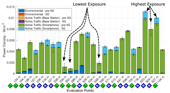
(a) Exposure Breakdown

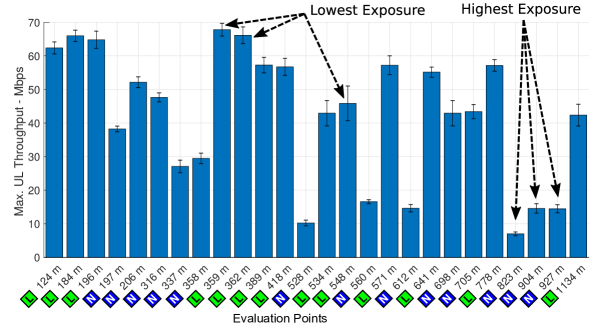
(b) Throughput Breakdown

Figure 13: Characterization of exposure (top) and throughput (bottom) over the outdoor evaluation points. The points are ordered from left to right by increasing distance values with respect to the 5G W3 installation. The sight condition (L=Line-of-Sight, N=Non-Line-Of-Sight) is also reported.

Eventually, the band index in Fig. 7 is initialized with the first UL bandwidth in which an increase of exposure was detected by the sel_band_use routine. Finally, the narrow band EMF measurement is realized through the nar_band_meas of Alg. 2, whose parameters for $P2$ are detailed in Tab. V on the right. The main difference w.r.t. $P1$ case relies on a different measurement metric, expressed in terms of [V/m]. In addition, the reference level set to 6 [V/m], since the measured signal levels are expected to be non-negligible. It is interesting to note that, when the [V/m] metric is set, the scale div are automatically tuned to show a minimum level of 0 [V/m], i.e., the minimum one. Eventually, the minimum and maximum frequency are set in accordance to the considered bandwidth, whose set is saved in the sel_band_array by the sel_band_use routine.

6.2.4 $P3$ Parameters

Focusing on the $P3$ assessment shown in Fig. 8, the initial band index is set with the first DL bandwidth of W3 in use by the data transfer (detected by sel_band_use function). The narrow band assessment reported in the second block of $P3$ adopts the same parameters of $P2$ (detailed in Tab. V on the right). Finally, the iperf transfer is turned off on the smartphone when all the bands in use have been considered.

6.3 Exposure Assessments

We initially concentrate on the outcomes from outdoor measurements of Fig. 9 and then we shed light on the results obtained in the indoor locations of Fig. 11.

6.3.1 Outdoor measurements

We run 5G-EA over the outdoor locations, by considering the generation of UL traffic from the smartphone to the iperf server. Fig. 13 reports the breakdown of exposure (top) and throughput (bottom). The exposure is expressed in terms of power density [W/m²], in order to display the different contributions (RBS vs. smartphone, active vs. environmental, pre-5G vs. 5G) over a stacked bar. Each exposure component is expressed in terms of average value over the collected samples. Moreover, the error bars report the confidence intervals, which are computed by assuming a Gaussian distribution with a confidence level of 95%.

We initially focus on the collected exposure values, shown in Fig. 13(a). Several considerations hold by analyzing in detail the figure. First, the active traffic exposure from the smartphone (pre-5G and 5G) dominates over all the other ones, in all the considered locations. Second, the RBS environmental exposure can be identified for all locations in LOS w.r.t. the RBS, while the same metric is negligible for all locations in NLOS. Third, the contribution of active traffic exposure from the RBS is almost imperceptible in all locations (except from two). Fourth, the majority of active traffic exposure from the smartphone is due to pre-5G contributions (mostly 4G), while 5G always represents a small share (at most equal to 38%) compared to the total one that is radiated by the smartphone. Fifth, NLOS locations generally present higher level of 5G exposure than LOS ones. Sixth, the increase of distance generally results in an increase of exposure (left to right of the figure). However, the largest exposure variations are observed between LOS and NLOS evaluation points. In particular, the latters exhibit a strong increase of active traffic exposure from the smartphone compared to the formers. As a side comment, the measured expsure levels are always orders of magnitude lower than the whole body and localized maximum power density values of ICNIRP guidelines [6].

In the following step, we compare the exposure of Fig. 13(a) against the achieved throughput levels shown in Fig. 13(b). Interestingly, a strong variation in the throughput levels is observed. We argue that this phenomenon is due to the different propagation conditions that are experienced in the measurement locations. To substantiate such observation, Fig. 13(a) highlights the three locations exhibiting the lowest exposure and the other three ones providing the highest exposure levels. Interestingly, the formers are in LOS, while the latters experience NLOS. When considering the throughput metric for the same locations (Fig. 13(b)), we can note that locations with lowest exposure (LOS) achieve very large throughput levels, typically larger than 45 [Mbps] in the UL, while the opposite holds for locations experiencing the highest exposure levels (NLOS), being the observed throughput lower than 16 [Mps]. Consequently, NLOS conditions are reflected into an increase of smartphone exposure and a degradation of throughput levels compared to LOS ones.

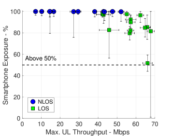
(a) Percentage of Smartphone Exposure vs. UL Throughput

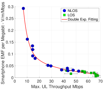
(b) Smartphone Exposure-per-Mbps vs. UL Throughput

Figure 14: Incidence of UL throughput on the smartphone active traffic exposure percentage (top) and on exposure-per-Mbps (bottom)

To provide more insights, Fig. 14(a) reports the percentage of active traffic exposure from the smartphone (w.r.t. the total one) vs. the observed throughput level. Each point in the figure corresponds to a measurement location (distinguished between LOS and NLOS), while x-y error bars are computed by assuming again 95% of confidence levels. Interestingly, we can note that the percentage of smartphone exposure is huge (close to 100%) for all the NLOS measurement locations. On the contrary, the percentage of smartphone exposure tends to decrease to lower levels for the LOS measurement locations. Moreover, a decrease is also observed when the realized UL throughput increases. In all the cases, however, the active traffic exposure from the smartphone is always higher than 50%, thus representing the largest source of exposure.

Having understood that there may be a strong relationship between the realized UL throughput and the collected exposure levels, we compute a novel metric, called smartphone exposure-per-Mbps, which is obtained by dividing the total exposure measured in the location by the observed throughput. The metric expresses the efficiency in terms of exposure (in [V/m]) for delivering a given amount of information (in [Mbps]). When the exposure-per-Mbps is high, the system is largely inefficient, as a huge exposure is needed to transfer the information. On the contrary, when the exposure-per-Mbps is low, the efficiency of the system in delivering the same amount of information is improved.

TABLE VII: Fitting parameters for the exposure estimator.

Parameter	Value
$F_{1}$	1.146 [V/m/Mbps]
$E_{1}$	-0.2595 [Mbps-1]
$F_{2}$	0.1304 [V/m/Mbps]
$E_{2}$	-0.0325 [Mbps-1]

Fig. 14(b) reports the smartphone exposure-per-Mbps vs. the observed throughput levels. Interestingly, the exposure-per-Mbps is inversely proportional to the throughput levels. The higher is the throughput, the flatter and closer to zero is the observed smartphone exposure-per-Mbps. On the contrary, the lower is the throughput, the higher is the asymptotic behavior of the exposure-per-Mbps, with the highest values observed for the lowest throughput levels. To better capture the aforementioned effects, we have applied the following double exponential fitting model:

$$C^{\text{EST}}=F_{1}\cdot e^{E_{1}\cdot T^{\text{UL}}}+F_{2}\cdot e^{E_{2}\cdot T^{\text{UL}}}$$ (2)

where $T^{\text{UL}}$ is the observed throghput level (in Mbps), $F_{1}$, $E_{1}$, $F_{2}$, $E_{2}$ are the fitting parameters (shown in Tab. VII) and $C^{\text{EST}}$ is the estimated smartphone exposure-per-Mbps.

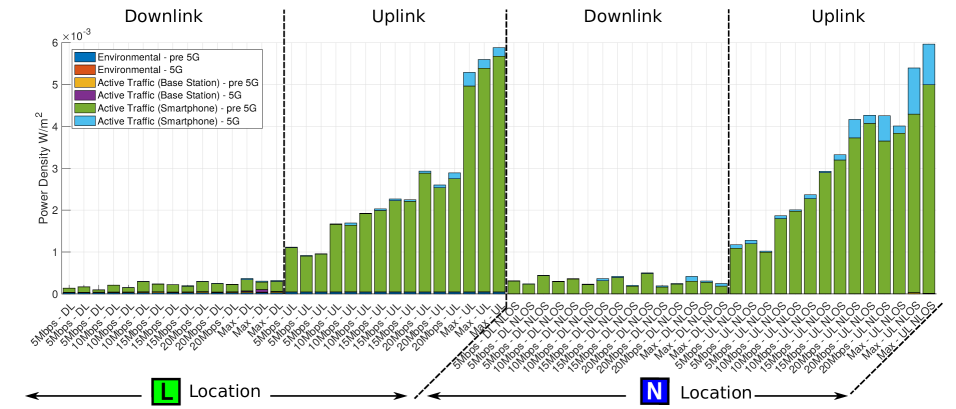
Figure 15: LOS/NLOS indoor locations: breakdown of exposure components vs. variation of UL/DL throughput.

By observing in detail Fig. 14(b) we can note that the realized UL throughput with iPerf tool can be used as an estimator of the smartphone exposure. In a practical scenario, the user could measure $T^{\text{UL}}$ by running an iPerf test in the UL direction and a given location. Then, the smartphone exposure could be retrieved by: i) applying the fitting model of Eq. (2) to compute $C^{\text{EST}}$, ii) computing the total estimated exposure as $C^{\text{EST}}\times T^{\text{UL}}$. Clearly, the values reported in Tab. 2 may depend on different metrics (like the smartphone model), whose impact on the fitting model (and consequently on the exposure levels) require further investigations as future work.

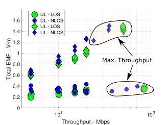
(a) Total EMF vs. throughput

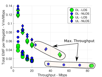
(b) Total Exposure-per-Mbps vs. throughput

Figure 16: LOS/NLOS indoor locations: total EMF and total exposure-per-Mbps vs. throughput.

6.3.2 Indoor measurements

In the following part of our work, we extend the results of the outdoor locations by investigating the exposure in the LOS/NLOS indoor locations. In particular, the availability of controlled environments allows performing extensive tests, in order to deeply analyze the impact of key parameteres on the exposure levels. To this aim, we initially focus on the impact of UL vs. DL traffic generation. For each location, we perform a wide range of UL and DL tests, including the variation of the generated traffic from very low values (set to 5 [Mbps]) up to the maximum one reachable on the wireless link (several dozens of Mbps). Moreover, three independent runs are executed for each parameter setting, in order to strengthen our outcomes.

Fig. 15 reports the breakdown of the exposure components for the considered tests. Four considerations hold by analyzing the figure. First, the exposure generated by the smartphone on pre-5G technologies dominates over the other components, both in the DL and in the UL. Second, the exposure in the DL is almost one order of magnitude lower than the one recorded in the UL tests. This is due to the fact that DL tests generate most of traffic flows from the Iperf server to the client, while a very low amount of information flows on the inverse direction (e.g., segment acknowledgements and/or control information). Third, the exposure tends to increase when the UL throughput is increased. Fourth, the exposure tends to be higher in the NLOS location than the LOS one, for a given level of generated traffic.

To better substantiate the previous findings, Fig. 16(a) details the total EMF vs. throughput over the two indoor locations. Interestingly, a strong increase of exposure is recorded when the UL traffic is increased, easily reaching values greater than 1 [V/m] (top part of the figure). Moreover, the difference between NLOS and LOS exposure tends to increase with increasing UL throughput. At last, when Iperf is set to generate the maximum traffic, the UL throughput in the NLOS location is clearly lower than the LOS one - despite the fact that the exposure values are comparable in both locations. A similar behaviour is also observed for the maximum traffic in the DL direction (bottom part of the figure). However, the increase of exposure due to traffic rising is less evident than in UL tests.

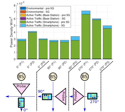
(a) Smartphone orientation variation with respect to the base station

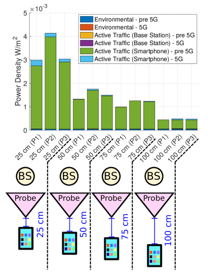
(b) EMF evaluation distance variation from the smartphone

Figure 17: Impact of smartphone orientation and EMF evaluation distance from the smartphone - LOS location with maximum UL traffic setting.

.

Eventually, Fig. 16(b) reports the total exposure-per-Mbps vs. throughput for the two locations and the UL/DL tests. Astonishingly, the inversely proportional law between exposure-per-Mbps and throughput clearly emerges in each location and in each direction. Given a location, the total exposure-per-Mbps is lower for the DL tests compared to the UL ones. Morever, given a direction of traffic generation, the total exposure-per-Mbps in NLOS tends to be higher than the one recorded in the LOS condition.

In the final part of our work, we evaluate the impact of changing the orientation and relative positioninig of the smartphone. Fig. 17(a) reports the exposure breakdown for each smartphone orientation setting reported on the bottom of the figure, corresponding to a smartphone rotation of $0^{\circ}$, $90^{\circ}$, $270^{\circ}$ in clockwise direction of the horizontal plane. For each angle, we perform three independent assessment with the maximum UL traffic. Interestingly, the dominance of smartphone exposure is evident in all the experiments. However, the $270^{\circ}$ rotation generally results in an higher exposure from the smartphone than the other angles. We argue that this phenomenon is due to the positioning of the smartphone main antenna on bottom right part the smartphone - opposite to the RBS when an angle of $270^{\circ}$ is set, which results in worse propagation conditions than the other settings.

Finally, we analyze the impact of increasing the distance of the exposure evaluation point w.r.t. the smartphone, as shown in Fig. 17(b). Starting from the default value of 0.25 [m], we increase the distance up to 1 [m]. As expected, the exposure experiences a sharp decrease when the distance is increased. However, we point out that the smartphone exposure is still the dominant component even when the distance is set to the maximum value of 1 [m].

7 Conclusions and Future Work

We have investigated the problem of exposure assessment in a commercial 5G network, by evaluating the impact of user generated traffic on the exposure from the RBS and the smartphone. To solve the complex and innovative measurement requirements - which include several aspects related to 5G implementation and its inter-viewing with legacy 4G networks - we have designed an innovative framework, called 5G-EA. Our framework splits the complex problem into a set of procedures, which are tailored to a specific measurement goal (environmental vs. active traffic assessment). In addition, 5G-EA relies on a completely softwarized approach, in which the measurement algorithm is run on a general purpose machine that controls the programmable spectrum analyzer.

We have then performed an extensive set of assessments in both outdoor and indoor locations. Interestingly, our results demonstrate that the smartphone contribution largely dominates over the other exposure components, particularly when UL traffic is injected. However, the largest contribution is due to pre-5G technologies, while 5G always constitute a small share (up to 38%) out of the total one that is radiated by the smartphone. In addition, the total exposure dramatically decreases when outdoor LOS conditions are experienced, and in general when the exposure from the RBS becomes detectable by the SAN. Moreover, we have designed and evaluated an exposure estimator based on the maximum UL traffic that is achieved by iPerf in the measurement location. Eventually, the exposure tends to increase in indoor locations when passing from LOS to NLOS condition, for a given level of UL traffic that is set towards the smartphone. Finally, we have demonstrated that the measured exposure levels are influenced by key parameters, like DL vs. UL direction, smartphone orientation and relative distance of the smartphone w.r.t. the measurement antenna.

We believe that our work paves the way for future research in the field. First, the application of 5G-EA in other deployments (e.g., subject to different exposure regulations and/or different radio configurations) is an interesting step. Second, the evaluation of exposure should be extended by considering multiple UE models/types, locations in balconies/terraces in close proximity to the serving RBS, and additional sources like WiFi. Third, the assessment of exposure in 5G deployments including mm-Wave frequencies is another line of research. Fourth, we plan to perform extensive assessment by running commonly used smartphone applications (social media, video streaming, online conference, etc.). Fifth, the decrease of exposure observed in LOS locations suggest that deploying a dense 5G network, in which most of territory is in LOS w.r.t. the serving RBS, is the best solution to reduce the exposure from the terminals. This goal could be alternatively achieved by installing intelligent surfaces (active or passive), to improve the signal coverage over the territory. The evaluation of exposure in such innovative deployments is therefore a future activity.

Luca Chiaraviglio (M’09-SM’16) received the Ph.D. degree in telecommunication and electronics engineering from the Polytechnic Unvisersity of Turin, Italy. He is currently an Associate Professor with the University of Rome “Tor Vergata”, Italy, teaching the courses of “Internet of Things” and “Networking and Internet”. He has co-authored more than 160 articles published in international journals, books, and conferences. His current research interests include 6G networks, electromagnetic fields assessments of 5G networks, and health risks assessment of 5G communications. He received the Best Paper Award at the IEEE Vehicular Technology Conference (VTC Spring), in 2020 and 2016, and at the Conference on Innovation in Clouds, Internet and Networks (ICIN), in 2018, all of them appearing as the first author. Some of his papers are listed as the Best Readings on Green Communications by the IEEE. Moreover, he has been recognized as an author in the top 1% most highly cited papers in the Information and Communication Technology (ICT) field worldwide and top 2% world scientists according to the 2021 and 2022 updates of the science-wide author databases of standardized citation indicators.

Chiara Lodovisi received the Ph.D. degree in engineering electronics from the University of Rome Tor Vergata, Italy. She worked for five years as a RF Engineer Consultant for H3G mobile operator and then as a Research Associate at the University of Rome Tor Vergata, focusing on optical communications, submarine and satellite optical links, and radio over fiber. She is currently a Researcher with CNIT, Italy. Her research interests include 5G networks, health risk assessment of 5G communications, interoperability over fiber between TETRA/LTE systems, and 5G networks.

Stefania Bartoletti received the Laurea degree (summa cum laude) in electronics and telecommunications engineering and the Ph.D. degree in information engineering from the University of Ferrara, Ferrara, Italy, in 2011 and 2015, respectively. She is currently Assistant Professor at the University of Rome “Tor Vergata”, Italy. She was a Marie Sklodowska-Curie Global Fellow within the Horizon 2020 European Framework for a research project with the Wireless Information and Network Sciences Laboratory, Massachusetts Institute of Technology (MIT), Cambridge, MA, USA, and the University of Ferrara during 2016-2019. Her research interests include theory and experimentation of wireless networks for passive localization and physical behavior analysis. Dr. Bartoletti was the recipient of the 2016 Paul Baran Young Scholar Award of the Marconi Society. She served as a Chair of the TPC for the IEEE ICC and Globecom Workshops on Advances in Network Localization and Navigation (ANLN) from 2017 to 2021, and as reviewer for numerous IEEE journals and international conferences. She is Editor of the IEEE Communications Letters.

Ahmed Elzanaty (Senior Member, IEEE) received the Ph.D. degree (cum laude) in electronics, telecommunications, and information technology from the University of Bologna, Italy, in 2018. He was a Research Fellow with the University of Bologna from 2017 to 2019. He was a Post-Doctoral Fellow with the King Abdullah University of Science and Technology, Saudi Arabia. He is currently a Lecturer (Assistant Professor) with the Institute for Communication Systems, University of Surrey, U.K. He has participated in several national and European projects, such as GRETA and EuroCPS. His research interests include cellular networks design with EMF constraints, coded modulation, compressive sensing, and distributed training of neural networks.

Mohamed Slim Alouini was born in Tunis, Tunisia. He received the Ph.D. degree in Electrical Engineering from the California Institute of Technology (Caltech) in 1998. He served as a faculty member at the University of Minnesota then in the Texas A&M University at Qatar before joining in 2009 the King Abdullah University of Science and Technology (KAUST) where he is now a Distinguished Professor of Electrical and Computer Engineering. Prof. Alouini is a Fellow of the IEEE and OPTICA (Formerly the Optical Society of America (OSA)). He is currently particularly interested in addressing the technical challenges associated with the uneven distribution, access to, and use of information and communication technologies in rural, low-income, disaster, and/or hard-to-reach areas.

References

- [1] How Many Smartphones Are in the World? Accessed: Oct. 4th, 2022. [Online]. Available: https://www.bankmycell.com/blog/how-many-phones-are-in-the-world.
- [2] Sales of 5G smartphone devices worldwide from 2019 to 2022. Accessed: Oct. 4th, 2022. [Online]. Available: https://www.statista.com/statistics/1220670/5g-smartphone-unit-sales-worldwide/.
- [3] 5G Global Launches & Statistics. Accessed: Oct. 4th, 2022. [Online]. Available: https://www.gsma.com/futurenetworks/ip_services/understanding-5g/5g-innovation/.
- [4] L. Chiaraviglio, A. Elzanaty, and M.-S. Alouini, “Health risks associated with 5G exposure: A view from the communications engineering perspective,” IEEE Open Journal of the Communications Society, vol. 2, pp. 2131–2179, 2021.
- [5] World Health Organization - ElectroMagnetic Fields. Available at https://www.who.int/health-topics/electromagnetic-fields, last accessed on 4th Oct 2022.
- [6] International Commission on Non-Ionizing Radiation Protection, “Guidelines for limiting exposure to electromagnetic fields (100 kHz to 300 GHz),” Health physics, vol. 118, no. 5, pp. 483–524, 2020.
- [7] J. Bushberg, C. Chou, K. Foster, R. Kavet, D. Maxson, R. Tell, and M. Ziskin, “IEEE Committee on Man and Radiation - COMAR Technical Information Statement: Health and safety issues concerning exposure of the general public to electromagnetic energy from 5G wireless communications networks,” Health Physics, vol. 119, no. 2, p. 236, 2020.
- [8] IEEE, “IEEE C95.1-2019 standard for safety levels with respect to human exposure to electric, magnetic, and electromagnetic fields, 0 Hz to 300 GHz,” IEEE Std., 2019.
- [9] A. Elzanaty, L. Chiaraviglio, and M.-S. Alouini, “5G and EMF exposure: Misinformation, open questions, and potential solutions,” Frontiers in Communications and Networks, vol. 2, p. 635716, 2021.
- [10] L.-M. Schilling, C. Bornkessel, and M. A. Hein, “Impact of Small-Cell Deployment on Combined Uplink and Downlink RF Exposure Compared to the Status Quo in Mobile Networks,” in 2021 51st European Microwave Conference (EuMC), pp. 618–621, IEEE, 2022.
- [11] L. Chiaraviglio, C. Lodovisi, D. Franci, S. Pavoncello, T. Aureli, N. Blefari-Melazzi, and M.-S. Alouini, “Massive Measurements of 5G Exposure in a Town: Methodology and Results,” IEEE Open Journal of the Communications Society, vol. 2, pp. 2029–2048, 2021.
- [12] G. Betta, D. Capriglione, G. Cerro, G. Miele, M. D. Migliore, and D. Šuka, “5G DSS communications: pilot signals’ variability analysis from measurements on the field,” in 2022 IEEE International Instrumentation and Measurement Technology Conference (I2MTC), pp. 1–6, IEEE, 2022.
- [13] G. Betta, D. Capriglione, G. Cerro, G. Miele, M. D. Migliore, and D. Suka, “Experimental analysis of 5G pilot signals’ variability in urban scenarios,” in 2022 IEEE International Symposium on Measurements & Networking (M&N), pp. 1–6, 2022.
- [14] M. S. Elbasheir, R. A. Saeed, and S. Edam, “Measurement and Simulation-based Exposure Assessment at a Far-Field for a Multi-Technology Cellular Site up to 5G NR,” IEEE Access, 2022.
- [15] C. Hausl, J. Emmert, M. Mielke, B. Mehlhorn, and C. Rowell, “Mobile Network Testing of 5G NR FR1 and FR2 Networks: Challenges and Solutions,” in 2022 16th European Conference on Antennas and Propagation (EuCAP), pp. 1–5, IEEE, 2022.
- [16] S. Adda, T. Aureli, S. D’elia, D. Franci, E. Grillo, M. D. Migliore, S. Pavoncello, F. Schettino, and R. Suman, “A theoretical and experimental investigation on the measurement of the electromagnetic field level radiated by 5G base stations,” IEEE Access, vol. 8, pp. 101448–101463, 2020.
- [17] S. Aerts, K. Deprez, D. Colombi, M. Van den Bossche, L. Verloock, L. Martens, C. Törnevik, and W. Joseph, “In Situ Assessment of 5G NR Massive MIMO Base Station Exposure in a Commercial Network in Bern, Switzerland,” Applied Sciences, vol. 11, no. 8, p. 3592, 2021.
- [18] M. D. Migliore, D. Franci, S. Pavoncello, E. Grillo, T. Aureli, S. Adda, R. Suman, S. D’Elia, and F. Schettino, “A New Paradigm in 5G Maximum Power Extrapolation for Human Exposure Assessment: Forcing gNB Traffic Toward the Measurement Equipment,” IEEE Access, vol. 9, pp. 101946–101958, 2021.
- [19] C. Bornkessel, T. Kopacz, A.-M. Schiffarth, D. Heberling, and M. A. Hein, “Determination of instantaneous and maximal human exposure to 5G massive-MIMO base stations,” in 2021 15th European Conference on Antennas and Propagation (EuCAP), pp. 1–5, IEEE, 2021.
- [20] L.-M. Schilling, C. Bornkessel, and M. A. Hein, “Analysis of Instantaneous and Maximal RF Exposure in 4G/5G Networks With Dynamic Spectrum Sharing,” in 2022 16th European Conference on Antennas and Propagation (EuCAP), pp. 1–5, IEEE, 2022.
- [21] L. Chiaraviglio, C. Lodovisi, D. Franci, S. Pavoncello, E. Merli, T. Aureli, N. Blefari-Melazzi, M. D. Migliore, and M.-S. Alouini, “EMF Exposure in 5G Standalone mm-Wave Deployments: What is the Impact of Downlink Traffic?,” IEEE Open Journal of the Communications Society, 2022.
- [22] S. Liu, T. Onishi, M. Taki, M. Ikuyo, K. Tobita, S. Watanabe, and Y. Suzuki, “E-Field Strength Measurements of a 5G Base Station in 28 GHz Band for EMF Exposure Assessment,” in 2021 IEEE USNC-URSI Radio Science Meeting (Joint with AP-S Symposium), pp. 49–50, IEEE, 2021.
- [23] F. Héliot, T. H. Loh, D. Cheadle, Y. Gui, and M. Dieudonne, “An Empirical Study of the Stochastic Nature of Electromagnetic Field Exposure in Massive MIMO Systems,” IEEE Access, vol. 10, pp. 63100–63112, 2022.
- [24] S. Aerts, L. Verloock, M. Van Den Bossche, D. Colombi, L. Martens, C. Törnevik, and W. Joseph, “In-situ measurement methodology for the assessment of 5G NR massive MIMO base station exposure at sub-6 GHz frequencies,” IEEE Access, vol. 7, pp. 184658–184667, 2019.
- [25] C. Chountala, J.-M. Chareau, and P. Chawdhry, “Radio Frequency Electromagnetic Field Measurements in a Commercial 5G Network,” in 2021 IEEE 4th 5G World Forum (5GWF), pp. 275–280, IEEE, 2021.
- [26] S. Q. Wali, A. Sali, J. K. Allami, and A. F. Osman, “RF-EMF Exposure Measurement for 5G Over Mm-Wave Base Station With MIMO Antenna,” IEEE Access, vol. 10, pp. 9048–9058, 2022.
- [27] B. Xu, K. Zhao, B. Thors, D. Colombi, O. Lundberg, Z. Ying, and S. He, “Power density measurements at 15 ghz for rf emf compliance assessments of 5g user equipment,” IEEE Transactions on Antennas and Propagation, vol. 65, no. 12, pp. 6584–6595, 2017.
- [28] M. Nedelcu, V. Niţu, and T. Petrescu, “Uplink power levels of user equipment in commercial 4G and 5G networks,” in 2021 13th International Conference on Electronics, Computers and Artificial Intelligence (ECAI), pp. 1–4, IEEE, 2021.
- [29] P. Joshi, F. Ghasemifard, D. Colombi, and C. Törnevik, “Actual output power levels of user equipment in 5G commercial networks and implications on realistic RF EMF exposure assessment,” IEEE Access, vol. 8, pp. 204068–204075, 2020.
- [30] A.-K. Lee, S.-B. Jeon, and H.-D. Choi, “EMF levels in 5G new radio environment in Seoul, Korea,” IEEE Access, vol. 9, pp. 19716–19722, 2021.
- [31] D.-B. Deaconescu, A. M. Buda, D. Vatamanu, and S. Miclaus, “The Dynamics of the Radiated Field Near a Mobile Phone Connected to a 4G or 5G Network,” Engineering, Technology & Applied Science Research, vol. 12, no. 1, pp. 8101–8106, 2022.
- [32] S. Miclaus, D.-B. Deaconescu, D. Vatamanu, A. M. Buda, A. Sarbu, and B. Pindaru, “Peculiarities of the radiated field in the vicinity of a mobile terminal connected to 4G versus 5G networks during various applications usage,” AIMS Electronics and Electrical Engineering, vol. 6, no. 2, pp. 161–177, 2022.
- [33] Resolution AGCOM n. 209/07/CONS - Procedures for the assignment of the right of use of frequencies for systems Broadband Wireless Access (BWA) in the spectrum at 3.5 GHz. (In Italian). Accessed: Oct. 4th, 2022. [Online]. Available: https://www.agcom.it/documents/10179/538341/Delibera+209-07-CONS/130848c5-7607-498a-a8ce-d5085e9ca996?version=1.0&targetExtension=pdf.
- [34] Resolution AGCOM n. 231/18/CONS - Procedures for the assignment and rules of the right of use of frequencies available in the 694-790 MHz, 3600-3800 MHz and 26.5-27.5 GHz for terrestrial systems of electronic communications to promote the transition towards 5G technology. (In Italian). Accessed: Oct. 4th, 2022. [Online]. Available: https://www.agcom.it/documents/10179/10517165/Delibera+231-18-CONS/ce5f9340-2b1f-49ba-9cd0-8984d9c56d85?version=1.0.
- [35] Resolution AGCOM n. 420/20/CONS - Application of the prevision art. 13, comma 14 of resolution n. 231/18/CONS to Wind Tre S.p.A. company. (In Italian). Accessed: Oct. 4th, 2022. [Online]. Available: https://www.agcom.it/documents/10179/20041149/Delibera+420-20-CONS/b4b41f9e-8296-4170-af42-670e03aa4da2?version=1.0.
- [36] M. Agiwal, H. Kwon, S. Park, and H. Jin, “A survey on 4G-5G dual connectivity: road to 5G implementation,” IEEE Access, vol. 9, pp. 16193–16210, 2021.
- [37] 5G NR User Equipment (UE) radio transmission and reception - Part 2: Range 2 Standalone (3GPP TS 38.101-2 version 17.5.0 Release 17). Available at https://www.etsi.org/deliver/etsi_ts/138100_138199/13810102/17.05.00_60/ts_13810102v170500p.pdf, last accessed on 15th June 2022.
- [38] Top 10 Smartphone Uses. Accessed: Oct. 16th, 2022. [Online]. Available: https://www.mobiles.co.uk/blog/top-10-smartphone-uses/.
- [39] IEC 62232:2017 Determination of RF Field Strength, Power Density and SAR in the Vicinity of Radiocommunication Base Stations for the Purpose of Evaluating Human Exposure. Accessed: Mar. 8th, 2022. [Online]. Available: https://webstore.iec.ch/publication/28673.