Nonlinear oscillators via Čebyšëv quintic approximations

Abstract

Aim of this work is the study of differential equations governing non–dissipative non–linear oscillators; these arise in different physical models such as the treatment of relativistic oscillators, from the first contribution due to [1] and the further analysis in [2], up to generalizations to Duffing’s relativistic oscillators [3]; they also appear in non–relativistic models as that in [4], which deals with cables with an attached midpoint mass, or some harmonic Duffing oscillators discussed in [5], [6] and [7]. From an exquisitely mathematical viewpoint, all these models, further than describing the one–dimensional motion of a particle, share being governed by the autonomous equation $\,\ddot{x}=f(x)\,$ where the restoring force is an odd function, and the consequent problem of inverting the associated time–integral; the latter can rarely be solved in explicit terms, excluding the well–known (both unforced) cases of pendulum and Duffing equations.

In this paper the inversion issue is treated by near–minimax approximation of the restoring force via fifth–order Čebyšëv polynomials, on a normalised integration interval: this allows time–integral inversion for the (generalised Duffing) quintic oscillator; in fact, the particular choice of orthogonal polynomials turns out to be very appropriate in yielding an approximate normalised system whose solutions effectively represent those of the original problem; moreover, when restoring forces are described by odd functions, the approximate equations are solvable in closed form via Jacobian elliptic functions.

1 Introduction

In this paper we present a method for determining analytic solutions to fifth–order approximations of non–linear oscillatory systems governed by odd functions, and consequently with even potential energy. The method described here is based on previous results regarding exact analytic solutions of quintic oscillators, due to [8], [9], [10], [11], [12], which are used by [13], and later by [14] and [15], to treat approximate models obtained via Čebyšëv polynomial up to degree five. Our method is applied to the relativistic oscillator proposed by McColl [1] and then studied in depth, with different techniques, in [2], [16], [17], [18]. We focus on solving non–linear differential equations, coupled to the originals ruling these models, using Čebyšëv approximants to their restoring force.

Among the techniques related to the study of non–linear oscillatory phenomena, we mention briefly the most popular: Lindstedt–Poincaré perturbation methods; multiple time–scale methods [19], [20], [21]; the generalised averaging method of Krylov, Bogoliubov and Mitropolski [22], [21]; the approximate variational method, or energy–balance [23], [24], to evaluate angular frequencies of non–linear oscillators; the harmonic–balance method [21], [25] [26], [27], [28], [29]. A notable source for Duffing oscillators is [30], while, for an overview of all these methods, we highlight [31], [25] and again [30]. The problem of period–amplitude dependence was analyzed in [32] through classical thermodynamic equilibrium theory, and an asymptotic estimate of period is obtained for the particular case of the predator–prey Volterra–Lotka model, which, after a suitable change of variable, is a conservative Hamiltonian system. This approach is extended to a wide class of Hamiltonian non–dissipative system in [33], via Laplace transform and asymptotic expansions.

The differential equations examined in this work are as follows:

$$\ddot{x}=-\dfrac{x}{\sqrt{1+x^{2}}}\;,$$ (1)

$$\qquad\ddot{x}=-x-\dfrac{b\;x}{\sqrt{1+x^{2}}}\;,\quad$$ (2)

$$\qquad\ddot{x}=-x-x^{3}-\dfrac{b\;x}{\sqrt{1+x^{2}}}\,.\quad$$ (3)

Equation (1) is related to the relativistic oscillator introduced in [1] and studied in depth in [2]. It is actually obtained from $\,\ddot{x}+(1-\dot{x}^{2})^{3/2}\;x=0\,$ studied in phase–space, after a change of variable; details are well–known and reported in several papers, such as the already mentioned [1], [2], and also [34], [16], [35].

Dynamics of cables with an attached midpoint mass are modeled by (2). We highlight the contributions of [36], [37], [38], [39], [3], [5], [7], where classical approximate analytic methods are employed through some algebraic procedures, such as an adapted variant of harmonic–balance.

The Duffing relativistic oscillator (3) is treated in [3] using He’s energy–balance method.

Differential equations (1)–(3) are all of the form $\,\ddot{x}=f(x)\,,$ where the restoring force $\,f\,$ is an odd continuous function. Assuming motion starts from rest, i.e. $\,\dot{x}(0)=0\,,$ and choosing an initial displacement $\,a>0\,$ so that $\,f(x)\neq 0\quad\forall x\in]0\,,a]\,,$ the resulting motion is periodic and the particle satisfies $\,-a\leq x(t)\leq a\;,\;\forall\,t\in\mathbb{R}\,.$ In other words, we study an initial value problem (IVP) of the form:

$$\begin{cases}\ddot{x}=f(x)\;,\\ x(0)=a\;,\quad\dot{x}(0)=0\;,\end{cases}$$ (4)

where $\,f:[-a\,,a]\to\mathbb{R}\,$ is continuous and such that $\,f(-x)=-f(x)\quad\forall x\in]0\,,a]\,;$ without loss of generality, $\,f(a)<0\,$ can be assumed. Now, let us introduce the even function:

$$\Phi(x):=-2\int_{x}^{a}f(s)\,{\rm d}s\;.$$ (5)

It is $\,\Phi(\pm a)=0\,,$ where both zeros are simple in the cases of our interest. Moreover:

$$\mathbb{T}=2\displaystyle\int_{-a}^{a}\;\dfrac{1}{\sqrt{\Phi(s)}}\;\;{{\rm d}s}$$ (6)

is the period of the solution to (4). This solution is implicitly defined for $\,|x|\leq a\,$ by the time–integral:

$$t\;\;=\;\Psi(x)\;,\qquad\qquad\qquad\Psi(x)\;:=\;\;\displaystyle\int_{x}^{a}\;\dfrac{1}{\sqrt{\Phi(s)}}\;\;{{\rm d}s}\;.$$ (7)

At this point, methods of approximation are necessary since the integral in (7) can rarely be evaluated first in closed form and then inverted, to yield $\;x\;\;=\;\Psi^{-1}(t)\;.\;$

Aim of this work is, namely, to provide the explicit solution, expressed via Jacobian elliptic functions, of an approximate problem, obtained by substituting the restoring force $\,f(x)\,$ with its fifth–order Čebyšëv polynomials of the first kind, due to their capability to provide good functions approximation.

As it is well–known, Čebyšëv’s are a numerable family of polynomials, orthogonal with respect to the weigth function $\,w(u)=1/\sqrt{1-u^{2}}\,,$ and defined for $\,-1\leq u\leq 1\,$ by the formulae:

$$T_{n}(u)=\cos\Big{(}n\;\;\arccos(u)\Big{)}=\;_{2}{\rm F}_{1}\left(\begin{matrix}n\;,-n\\ \dfrac{1}{2}\end{matrix}\;\left|\;\dfrac{1}{2}\,(1-u)\right.\right)\qquad\qquad n\in\mathbb{N}\;.$$

Here $\,{}_{2}{\rm F}_{1}\,$ denotes the Gauss hypergeometric function [40].

Čebyšëv polynomials form a complete orthogonal set on $\,[-1\,,1]\,$ in the appropriate Sobolev space, thus a function $\,g(u)\,$ can be expressed on its domain $\,[-1\,,1]\,$ via the expansion:

$$g(u)=\tilde{g}(u)+E_{r}(u)\;,\qquad\tilde{g}(u):=\dfrac{1}{2}\;\alpha_{0}+\displaystyle\sum_{n=1}^{r}\;\alpha_{n}\;T_{n}(u)\;,\qquad E_{r}(u):=\displaystyle\sum_{n=r+1}^{\infty}\;\alpha_{n}\;T_{n}(u)\;.$$ (8)

If $\,g\,$ is Lipschitz continuous on $\,[-1\,,1]\,,$ then it has a unique representation as the infinite Čebyšëv series (8), which is absolutely and uniformly convergent, with coefficients defined using the weighted inner product [41]:

$$\alpha_{0}=\dfrac{1}{\pi}\;\displaystyle\int_{-1}^{1}\;\dfrac{1}{\sqrt{1-s^{2}}}\;\;T_{n}(s)\;\;g(s)\;\;{\rm d}s\;,\qquad\quad\displaystyle\alpha_{n}=\dfrac{2}{\pi}\;\displaystyle\int_{-1}^{1}\;\dfrac{1}{\sqrt{1-s^{2}}}\;\;T_{n}(s)\;\;g(s)\;\;{\rm d}s\;\,\quad\mbox{for}\quad n\geq 1\,.$$

Recall that it is $\,|T_{n}(u)|\leq 1\;\;\forall u\in[-1\;,1]\,.$ Moreover, $\,T_{n}(u)\,$ has $\,n\,$ distinct real roots in $\,]-1\,,1[\,,$ and it has $\,n+1\,$ extrema in $\,[-1\,,1]\,$ at which it takes alternating values $\,\pm 1\,.$ Thus, if coefficients $\,\alpha_{n}\,$ decrease in magnitude sufficiently rapidly (which depends on regularity of $\,g\,$), then $\;E_{r}(u)\simeq\alpha_{r+1}\;T_{r+1}(u)\;$ equioscillates $\,r+2\,$ times on $\,[-1\,,1]\,,$ implying that $\,\tilde{g}\,$ is a near–minimax approximant for $\,g\,$ [42]. Coefficients $\,\alpha_{n}\,$ can be determined explicitly for some functions, otherwise they need discretisation via quadrature formulae. Even so, among methods yielding minimax or near–minimax approximations, Čebyšëv series are effective and easy to handle.

To apply Čebyšëv approximation to the nonlinear oscillators under study, the displacement $\,a\,$ is normalised to the interval $\,[-1\;,1]\;$ via a change of dependent variable $\,u=x/a\,,$ and the following equivalent IVP is considered in place of (4):

$$\begin{cases}\ddot{u}=f_{a}(u)\;,\qquad\qquad\qquad\qquad\qquad\qquad f_{a}(u):=\dfrac{1}{a}\;\;f(a\,u)\;,\\ u(0)=1\;,\quad\dot{u}(0)=0\;.\end{cases}$$ (9)

We then choose to describe the normalised restoring force $\,f_{a}(u)\,,$ which is an odd function, in terms of polynomials $\,T_{n}(u)\,;$ for our purposes, $\,f_{a}(u)\,$ is expanded in Čebyšëv series truncated (or projected) at fifth–order:

$$f_{a}(u)\,\simeq\,\tilde{f}_{a}(u):=\alpha_{1}\,T_{1}(u)+\alpha_{3}\,T_{3}(u)+\alpha_{5}\,T_{5}(u)\;,$$ (10)

where:

$$T_{1}(u)=u\;,\qquad T_{3}(u)=-3\,u+4\,u^{3}\;,\qquad T_{5}(u)=5\,u-20\,u^{3}+16\,u^{5}\;,$$

and

$$\alpha_{n}=\dfrac{2}{\pi}\;\displaystyle\int_{-1}^{1}\;\dfrac{1}{\sqrt{1-s^{2}}}\;\;T_{n}(s)\;\;f_{a}(s)\;\;{\rm d}s\;,\qquad\qquad n=1\,,3\,,5\,.\quad$$ (11)

Expressing the approximate normalised force $\,\tilde{f}_{a}(u)\,$ in the monomial base, a new IVP replaces (9):

$$\begin{cases}\ddot{u}=-(c_{1}\;u+c_{3}\;u^{3}+c_{5}\;u^{5})\;,\\ u(0)=1\;,\quad\dot{u}(0)=0\;,\end{cases}$$ (12)

where, setting $\;\mathcal{C}=-2^{5}/\pi\,:$

$$c_{1}=-(\alpha_{1}-3\,\alpha_{3}+5\,\alpha_{5}) = \mathcal{C}\;\int_{-1}^{1}\;\dfrac{1}{\sqrt{1-s^{2}}} (\dfrac{35}{16}\,s-7\,s^{3}+5\,s^{5}) f_{a}(s) {\rm d}s\;,$$ (13)

$$c_{3}=-4\,(\alpha_{3}-5\,\alpha_{5}) = \mathcal{C}\;\int_{-1}^{1}\;\dfrac{1}{\sqrt{1-s^{2}}} (-7\,s+26\,s^{3}-20\,s^{5}) f_{a}(s) {\rm d}s\;,$$

$$c_{5}=-16\,\alpha_{5} = \mathcal{C}\;\int_{-1}^{1}\;\dfrac{1}{\sqrt{1-s^{2}}} (5\,s-20\,s^{3}+16\,s^{5}) f_{a}(s) {\rm d}s\;.$$

In $\S$ 2, a novel solution procedure is presented for the general quintic oscillator (12) in terms of Jacobian elliptic functions, leading to the determination of exact periods and frequencies. In $\S$ 3, the solution process is illustrated on the relativistic oscillator (1): its normalised and quinticated approximation is built and the exact integration obtained in $\S$ 2 is applied to solve it; quality of the results obtained is also validated. In $\S$ 4, a similar application to oscillators (2) and (3) proves both feasibility and robustness of the solution process introduced. The conclusive $\S$ 5 reports some final comments and indications for future work.

2 General quintic oscillator

Consider the family of IVPs (12). We highlight several contributions for this kind of problems due to [9], [8], [43], [44], [10], [45], [12], [11]. Application of (5) and (7) to the approximate normalised force in (12) shows that the (squared) solution of this IVP is based on the evaluation of an elliptic integral:

$$t=\sqrt{\frac{3}{2}}\;\;\displaystyle\int_{u^{2}}^{1}\;\;\dfrac{1}{\sqrt{s\;\left(1-s\right)\;h_{2}(s)}}\quad{{\rm d}s}\;,$$ (14)

with

$$h_{2}(s)=(6\,c_{1}+3\,c_{3}+2\,c_{5})+\left(3\,c_{3}+2\,c_{5}\right)\,\,s+2\,c_{5}\,s^{2}\;.$$

The discriminant of polynomial $\,h_{2}(s)\,$ is, discarding a factor of value $\,3\,:$

$$\Delta=3\,c_{3}^{2}-4\,c_{5}\,\left(4\,c_{1}+c_{3}+c_{5}\right)\;.$$ (15)

Given the physical nature of the restoring forces acting in the models of interest, coefficients $\,c_{1}\,,c_{3}\,,c_{5}\,$ can be assumed to be such that $\,h_{2}(s)>0\quad\forall s\in(0\,,1)\,.$ This property is assured if $\,c_{5}>0\,$ together with one of the two conditions:

$$\mbox{(i)}\quad\Delta\leq 0\;;\qquad\qquad\qquad\mbox{(ii)}\quad\Delta>0\,\quad\mbox{and}\quad\,6\,c_{1}+3\,c_{3}+2\,c_{5}>0\,.\qquad$$ (16)

The following Theorems 2.1 and 2.2 provide closed–form solution and period for (12), respectively under conditions (i) or (ii). Notice that, in the latter case, the roots of $\,h_{2}(s)\,,$ further than being real and distinct, are both negative, due to Descartes’ rule of signs. Solution of (12) has a cosine wave behaviour, as Figure 1 illustrates for the example case $\,c_{1}=1\;,$ $c_{3}=2\;,$ $c_{5}=3\;.$

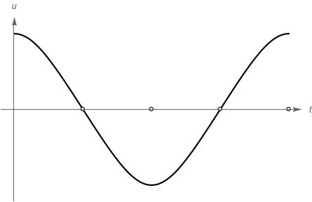
Figure 1: Plot of the solution to IVP (12) for $\,c_{1}=1\;,c_{3}=2\;,c_{5}=3\,,\,$ in one period interval

Theorem 2.1.

Given the time–integral (14), assume $\,c_{5}>0\,$ and $\,\Delta\leq 0\,$ in (15), and define:

$$A=\dfrac{\sqrt[4]{6}}{2}\;\;\dfrac{1}{\sqrt[4]{\mathcal{P}\;\;\mathcal{Q}}}\;,\qquad\qquad B=\dfrac{1}{6}\;\dfrac{\mathcal{Q}}{\mathcal{P}}\;,\qquad\qquad\qquad k^{2}=\dfrac{1}{2}-\dfrac{\sqrt{6}}{8}\;\dfrac{\mathcal{K}}{\sqrt{\mathcal{P}\;\;\mathcal{Q}}}\;,$$ (17)

with

$$\mathcal{P}=c_{1}+c_{3}+c_{5}\;,\qquad\qquad\mathcal{Q}=6\,c_{1}+3\,c_{3}+2\,c_{5}\;,\qquad\qquad\mathcal{K}=4\,c_{1}+3\,c_{3}+2\,c_{5}\;.$$ (18)

Then, the solution of IVP (12) is:

$$u^{2}(t)=\dfrac{\sqrt{B}}{\sqrt{B}+\cot^{2}\Bigg{(}\dfrac{1}{2}\;\;{\rm am}\left(2\;\mathbf{K}(k)-\dfrac{t}{A}\;,\;k\right)\Bigg{)}}\;.$$ (19)

where $\,{\rm am}(s\,,k)\,$ indicates the Jacobi amplitude function, i.e. the inverse of the elliptic integral of first kind $\,F(\varphi\,,k)\,,$ meaning that $\,\varphi={\rm am}(s\,,k)\;$ iff $\;s=F(\varphi\;,k)\;,$ where:

$$F(\varphi\;,k)\;:=\;\displaystyle\int_{0}^{\sin(\varphi)}\;\dfrac{1}{\sqrt{(1-s^{2})\;(1-k^{2}\;s^{2})}}\;\;{\rm d}s\;,\qquad\qquad-\dfrac{\pi}{2}<\varphi<\dfrac{\pi}{2}\;,$$ (20)

while $\,\mathbf{K}(k)\,\;:=\;F(\dfrac{\pi}{2}\;,k)\;$ denotes the complete elliptic integral of first kind, with elliptic modulus $\,k\,.$

Solution (19) is periodic, with period:

$$\mathbb{T}=8\,\;A\,\;\mathbf{K}(k)\;,$$ (21)

and it is positive for $\,0\leq t\leq\dfrac{1}{4}\,\mathbb{T}\;,\quad\dfrac{3}{4}\,\mathbb{T}\leq t\leq\mathbb{T}\,,$ while it is negative for $\,\dfrac{1}{4}\,\mathbb{T}<t<\dfrac{3}{4}\,\mathbb{T}\,.$

Proof.

The integral in (14) can be evaluated using entry 3.145–2 in [46], recalled here:

$$\int_{\beta}^{v}\;\dfrac{1}{\sqrt{(\eta-s)\;(s-\beta)\;\;\big{(}(s-m)^{2}+n^{2}\big{)}}}\;{\rm d}s\;=\;\dfrac{1}{\sqrt{p\,q}}\,F(\varphi(v)\;,k)\;,$$ (22)

where:

$$\beta<v<\eta\;,\qquad\quad p^{2}:=(m-\eta)^{2}+n^{2}\;,\quad\qquad q^{2}:=(m-\beta)^{2}+n^{2}\,,$$

and

$${\varphi(v)=2\,{\rm arccot}\sqrt{\dfrac{q\;(\eta-v)}{p\;(v-\beta)}}}\;,\qquad\displaystyle{k^{2}=\dfrac{1}{4}\,\dfrac{(\eta-\beta)^{2}-(p-q)^{2}}{p\;q}}\;.$$

In the case of (14), $\,\beta=0\;,\,\eta=1\;,v=u^{2}\;,$ and polynomial $\,h_{2}(s)\,$ is rearranged as:

$$\dfrac{1}{2\;c_{5}}\;\;h_{2}(s)\;=\;\Bigg{(}s\;+\;\Big{(}\dfrac{3\,c_{3}}{4\;c_{5}}\;+\;\dfrac{1}{2}\Big{)}\Bigg{)}^{2}\;+\;\Bigg{(}\dfrac{3\,c_{1}}{c_{5}}\;-\;\Big{(}\dfrac{3\,c_{3}}{4\;c_{5}}\Big{)}^{2}\;+\;\dfrac{3\,c_{3}}{4\;c_{5}}\;+\;\dfrac{3}{4}\Bigg{)}\,.$$

To apply formula (22), the integral in (14) must further be rewritten as the difference of integrals of the same integrand on intervals $\,[0\,,1]\,$ and $\,[0\,,u^{2}]\,.$ Equation (14) thus becomes:

$$t=2\;\;A\;\;\mathbf{K}(k)-A\;\;F\Bigg{(}2\;{\rm arccot}\left(\sqrt[4]{B}\;\;\sqrt{\Upsilon(u^{2})}\right)\;,\;k\Bigg{)}\;,$$ (23)

where $\,\Upsilon(v)=(1-v)/v\,.$ At this point, due to invertibility of the elliptic integral of first kind, inversion of the time–integral equation (23) is possible, and it yields solution (19). In a similar way, (21) can be proved to provide the motion period. ∎

Theorem 2.2.

Given the time–integral (14), assume $\,c_{5}>0\,$ and condition (ii) in (16), that is $\;h_{2}(s)=(s-s_{1})\,(s-s_{2})\;$ where $\,s_{1}<s_{2}<0\,$ are its real roots. Now, define:

$$k^{2}=\dfrac{s_{2}-s_{1}}{s_{1}\left(s_{2}-1\right)}\;.$$ (24)

Then, the solution of IVP (12) is:

$$u^{2}(t)=s_{1}+\dfrac{s_{1}\;(s_{1}-1)}{{\rm sn}^{2}\left(\sqrt{\dfrac{c_{5}\;s_{1}\;\left(s_{2}-1\right)}{3}}\;\;\;t\;,\;\;k\right)-s_{1}}\;,$$ (25)

where $\,{\rm sn}(s\,,k)\,$ is the Jacobi sine amplitude function, i.e. $\,{\rm sn}(s\,,k)=\sin(\varphi)\,,$ with $\,\varphi={\rm am}(s\,,k)\,.$

Solution (25) is periodic, with period:

$$\mathbb{T}=\dfrac{4\;\sqrt{3}}{\sqrt{c_{5}\;s_{1}\;\left(s_{2}-1\right)}}\;\;\mathbf{K}\left(k\right)\;,$$ (26)

and it is positive for $\,0\leq t\leq\dfrac{1}{4}\,\mathbb{T}\;,\;\;\dfrac{3}{4}\,\mathbb{T}\leq t\leq\mathbb{T}\,,$ while it is negative for $\,\dfrac{1}{4}\,\mathbb{T}<t<\dfrac{3}{4}\,\mathbb{T}\,.$

Proof.

To evaluate the integral in (14), entry 3.147–7 of [46] is used, recalled below:

$$\int_{v}^{\eta}\dfrac{{\rm d}s}{\sqrt{(\eta-s)\,(s-\beta)\,(s-\gamma)\,(s-\delta)}}=\dfrac{2}{\sqrt{(\eta-\gamma)\,(\beta-\delta)}}\;\;F(\varphi(v),k)\;,$$

where:

$$\delta<\gamma<\beta\leq v<\eta\;,\qquad\varphi(v)=\arcsin\sqrt{\dfrac{(\beta-\delta)(\eta-v)}{(\eta-\beta)(v-\delta)}}\,,\qquad k^{2}=\dfrac{(\eta-\beta)(\gamma-\delta)}{(\eta-\gamma)(\beta-\delta)}\;.$$

In the case of (14), $\,\beta=0\,,\eta=1\,,\,v=u^{2}\,,\,\gamma=s_{2}\,,\,\delta=s_{1}\;.$ Thus, the motion period is given by (26), while (25) provides the solution, after the relevant computations, not reported here, as they are similar to those performed in proving Theorem 2.1. ∎

If $\,\Delta=0\,,$ integral (14) degenerates into an elliptic integral of third kind, which is tabulated as entry 3.138–6 of [46]. Here, the related computation are omitted for two reasons. First of all, condition $\,\Delta=0\,$ is linked to a very particular value of the initial displacement $\,a\,.$ Secondly, even though the appareance of elliptic integrals of third kind makes it impossible to invert the time–integral and compute the solution explicitly, thanks to the continuous dependence on data, the relevant solution can be approximated at arbitrary precision with solutions obtained in Theorems 2.1 and 2.2.

3 Application to the relativistic oscillator

In the case of the relativistic oscillator ruled by (1) the normalised equation is:

$$\begin{cases}\ddot{u}=-\dfrac{u}{\sqrt{1+a^{2}\;\;u^{2}}}\;,\\ u(0)=1\,,\quad\dot{u}(0)=0\;.\end{cases}$$ (27)

Here, function $\,\Phi(u)\,,$ defined in (5), becomes:

$$\Phi(u)=\dfrac{2}{a^{2}}\,\Big{(}\sqrt{1+a^{2}}-\sqrt{1+a^{2}\;u^{2}}\Big{)}\,,$$ (28)

while, after some algebraic adjustments, function $\,\Psi(u)\,,$ defined in (7), is:

$$\begin{split}\Psi(u)&=\frac{a}{\sqrt{2}\;\;\sqrt[4]{1+a^{2}}}\;\;\int_{u}^{1}\;\dfrac{1}{\sqrt{1-\sqrt{\dfrac{1+a^{2}\;s^{2}}{1+a^{2}}}}}\;\;\;{\rm d}s\\ &=\dfrac{\sqrt[4]{1+a^{2}}}{\sqrt{2}}\;\;\int_{{}_{\sqrt{\frac{1+a^{2}\;u^{2}}{1+a^{2}}}}}^{1}\qquad\dfrac{z}{\sqrt{(1-z)\left(z^{2}-\dfrac{1}{1+a^{2}}\right)}}\;\;{\rm d}z\;,\end{split}$$ (29)

where it is, obviously, $\;0<\frac{1}{\sqrt{1+a^{2}}}<\sqrt{\frac{1+a^{2}\;u^{2}}{1+a^{2}}}<1\;.$ The integral in (29) can be expressed in explicit form, for example via entry 3.132–5 of [46], through which the time equation (7) becomes:

$$t=\sqrt{2}\;\;\Bigg{(}\mathcal{A}\;\;E\left(\varphi,k\right)-\dfrac{F\left(\varphi,k\right)}{\mathcal{A}}\Bigg{)}\;,\qquad\qquad\mathcal{A}=\sqrt{\sqrt{1+a^{2}}+1}\;,$$ (30)

being $\,F\left(\varphi,k\right)\,$ and $\,E\left(\varphi,k\right)\,$ elliptic integrals of first and second kind, with:

$$\varphi=\arcsin\sqrt{\frac{\sqrt{1+a^{2}}-\sqrt{1+a^{2}\;u^{2}}}{\sqrt{1+a^{2}}-1}}\,,\qquad\qquad k=\dfrac{\sqrt{1+a^{2}}-1}{a}\;.$$ (31)

Note that, for any $\,a>0\;,$ the elliptic modulus $\,k\,$ satisfies the requirement $\,k<1\;.$

Calculation of the integral in (29) further leads to the exact determination of the period of oscillation:

$$\mathbf{T}=4\,\sqrt{2}\;\;\Bigg{(}\mathcal{A}\;\;\mathbf{E}(k)-\dfrac{\mathbf{K}(k)}{\mathcal{A}}\Bigg{)}\;,\qquad\qquad\mathcal{A}=\sqrt{\sqrt{1+a^{2}}+1}\;,$$ (32)

where $\mathbf{K}(k)$ and $\mathbf{E}(k)$ are the complete elliptic integrals of first and second kind, respectively, with modulus $k$ as in (31). The explicit formula (32) for the period of the relativistic oscillator is useful in itself, and also because it allows a comparison with the period of the approximated quintic oscillator we are to obtain.

Deriving solution $\,u\,$ from (30), in fact, poses the computational problem represented by inversion of the time–integral. We then, instead, approximate the normalised restoring force in (27), using Čebyšëv polynomials and expressing it in the monomial base through coefficients $\,c_{1}\,,c_{3}\,,c_{5}\,$ given by (13): according to the sign of the $\,\Delta\,$ discriminant built on such coefficients, the seeked solution is (19) or (25).

Application of formulae (13) to the considered problem (27) suggests to introduce three elliptic integrals:

$$J_{n}(a)=\int_{-1}^{1}\;\dfrac{s^{n}}{\sqrt{\left(1-s^{2}\right)\left(1+a^{2}\;s^{2}\right)}}\,{\rm d}s\;,\qquad n=2\,,4\,,6\;.$$

since, setting $\;\mathcal{C}=2^{5}/\pi\,:$

$$c_{1} =\mathcal{C}\;\Big{(}\dfrac{35}{16}\,J_{2}(a)-7\,J_{4}(a)+5\,J_{6}(a)\Big{)}\;,$$ (33)

$$c_{3} =\mathcal{C}\;\left(-7\,J_{2}(a)+26\,J_{4}(a)-20\,J_{6}(a)\right)\;,$$

$$c_{5} =\mathcal{C}\;\left(5\,J_{2}(a)-20\,J_{4}(a)+16\,J_{6}(a)\right)\;.$$

Using entries 236.16 and 331.01–03 of [47], it follows:

$$J_{2}(a) =\dfrac{2}{a^{2}}\;\Big{(}\mathcal{J}\;\;\mathbf{E}(h^{2})\;-\;\dfrac{1}{\mathcal{J}}\;\;\mathbf{K}(h^{2})\Big{)}\;,$$ (34)

$$J_{4}(a) =\dfrac{2}{3\;a^{4}}\;\Big{(}2\;(a^{2}-1)\;\;\mathcal{J}\;\;\mathbf{E}(h^{2})\;-\;(a^{2}-2)\;\;\dfrac{1}{\mathcal{J}}\;\;\mathbf{K}(h^{2})\Big{)}\;,$$

$$J_{6}(a) =\dfrac{2}{15\,a^{6}}\;\Big{(}(8\,a^{4}-7\,a^{2}+8)\;\;\mathcal{J}\;\;\mathbf{E}(h^{2})\;-\;(4\,a^{4}-3a^{2}+8)\;\;\dfrac{1}{\mathcal{J}}\;\;\mathbf{K}(h^{2})\Big{)}\;,$$

where $\,\mathcal{J}=\sqrt{1+a^{2}}\,$ and the elliptic modulus is given by $\,h=a/\mathcal{J}\,.$

It is thus possible to identify closed–form expressions for coefficients $\,c_{1}\,,c_{3}\,,c_{5}\,$ of the approximate quintic oscillator, inserting values (34) of integrals $\,J_{2}\,,J_{4}\,,J_{6}\,$ into (33).

The consequent expression (15) of the $\,\Delta\,$ discriminant is complicated, but still tractable using computer algebra systems, such as Mathematica [48], within which various graphical tools are also provided, enabling a visual analysis as that shown in Figure 2.

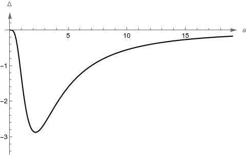
Figure 2: Discriminant $\,\Delta=\Delta(a)\,$ associated to the quinticated form of oscillator (1)

At this point, knowing that $\,\Delta\leq 0\,,$ solution and period are those given in Theorem 2.1; condition $\,c_{5}>0\,$ can, indeed, also be checked, for example via built–in visualisation resources. This whole process indeed involves complicated expressions which, however, remain manageable using computer algebra.

What is important to note is that, in order to use the procedure presented, what is ultimately needed is to calculate the integrals expressing the orthogonal projection onto the space of Čebyšëv polynomials. From that point on, by means of the coefficients of the quintic polynomial that approximates the normalised restoring force and by Theorem 2.1, or if appropriate Theorem 2.2, one arrives at the approximate solution and its period.

To validate the quality of the approximation obtained, the computational capacity of Mathematica can again be exploited in evaluating the differential operator:

$$L\,u=\ddot{u}\,-\,f_{a}(u)\,,$$ (35)

where here it is $\,f_{a}(u)=-{u}/{\sqrt{1+a^{2}\;u^{2}}}\,,$ since we are studying oscillator (1), while $\,f_{a}(u)=f_{a}(u\,,b)=-u-{b\,u}/{\sqrt{1+a^{2}\;u^{2}}}\,$ for oscillator (2) and $\,f_{a}(u)=f_{a}(u\,,b)=-u-a^{2}\,u^{3}-{b\,u}/{\sqrt{1+a^{2}\;u^{2}}}\,$ for oscillator (3), as we will see in $\S$ 4.1 and $\S$ 4.2 respectively.

For the quinticated IVP associated to oscillator (1), Figure 3 reports the graph of the deviation from zero produced in (35) by solution $\,u\,$ in the first quarter of the period, and at initial displacements equal to $\,a=1,\,2,\,3\,$ and $\,a=8,\,20,\,30\,;$ plots are kept separate for effective rendering reasons.

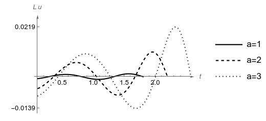
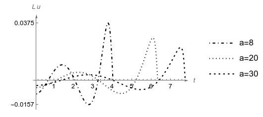
Figure 3: Behaviour of $\,L\,u\,,$ where $\,u\,$ is solution (19) with coefficients (33), for the quinticated form of oscillator (1)

It is reasonable for the approximation to initially get worse as the displacement increases, given the normalisation of the integration interval. However, computation of the maximum difference in the first quarter of the period yields results in Table 1, showing that an upper bound is given by the value $\,0.0375439\,$ (approximatively and working in machine precision) reached at $\,a=8\,,$ from where a monotonic decrease can be observed.

a	1	2	3	8	20	30
$\|L\,u\|_{\infty}$	.0013005	.0109030	.0219219	.0375439	.0278857	.0216839

Table 1: Uniform norm of $\,L\,u\,,$ where $\,u\,$ is solution (19) with coefficients (33), for the quinticated form of oscillator (1)

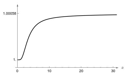
Figure 4: Period ratio in the case of the quinticated form of oscillator (1)

The validity of the quintic approximations is further testified by the ratio between exact period (32) of the gravitational oscillator and period (21) of the approximation: this ratio remains close to $\,1\,,$ and bounded above by the value $1.00058\,$ for large values of $\,a\,.$ Figure 4 illustrates the ratio behaviour for displacements up to $\,a=30\,.$

4 Quinticated oscillators

Here, the procedure introduced in $\S$ 2 is applied to the conservative non–linear oscillatory system (2) and the Duffing relativistic oscillator (3). Results obtained are wholly analogous to those seen for the relativistic oscillator (1). In particular, it is still possible to determine closed–form expressions for the coefficients of the Čebyšëv quintic approximant, in terms of complete elliptic integrals of first and second kind.

4.1 Nonlinear oscillator (2)

The normalised IVP, here, is:

$$\begin{cases}\ddot{u}=-u-\dfrac{b\;u}{\sqrt{1+a^{2}\;\;u^{2}}}\;,\\ u(0)=1\,,\quad\dot{u}(0)=0\;,\end{cases}$$ (36)

thus function $\,\Phi(u)\,,$ defined in (5), becomes:

$$\Phi(u)=1-u^{2}+\dfrac{2\,b}{a^{2}}\,\Big{(}\sqrt{1+a^{2}}-\sqrt{1+a^{2}\;u^{2}}\Big{)}\,,$$ (37)

so that forming $\,\Psi(u)\,$ as in (7) requires $\,2\,b>\sqrt{1+a^{2}}-\sqrt{1+a^{2}\,u^{2}}>0\,,$ being $\,a>0\,$ and $\,0<u<1\,.$

The exact period in this case, obtained using entry 3.148–7 in [46], is:

$$\mathbf{T}=\dfrac{4}{\sqrt{\mathcal{A}}}\;\;\Bigg{(}(1+\sqrt{1+a^{2}})\;\;\;\mathbf{\Pi}\left(\mathcal{N}\;,\;\mathcal{K}\right)\;-\;\;\mathbf{K}(\mathcal{K})\Bigg{)}$$ (38)

with

$${\mathcal{A}}=\sqrt{1+a^{2}}+b\;,\qquad\qquad\mathcal{N}=\dfrac{1-\sqrt{1+a^{2}}}{2}\;,\qquad\qquad{\mathcal{K}}=\dfrac{\mathcal{N}\;\;(b-\mathcal{N})}{\mathcal{A}}\;.$$

$\mathbf{K}(\mathcal{K})$ and $\mathbf{\Pi}(\mathcal{N}\;,\;\mathcal{K})$ are the complete elliptic integrals of first and third kind, respectively, where $\,\mathcal{N}\,$ is the elliptic characteristic, while the modulus satisfies $\,\mathcal{K}<1\,$ for $\,a\,,b>0\,.$

For system (36), given the exact computation of integrals (34), the three coefficients of the quinticated approximant can also be computed explicitly, using again (13), recalled here for reading convenience:

$$c_{1}=-(\alpha_{1}-3\,\alpha_{3}+5\,\alpha_{5})\;,\qquad c_{3}=-4\;(\alpha_{3}-5\,\alpha_{5})\;,\qquad c_{5}=-16\;\alpha_{5}\;,$$

where, setting $\,\mathcal{C}=-2/\pi\;:$

$$\alpha_{1} =\phantom{111}\mathcal{C}\;\Big{(}w_{2}+b\;J_{2}(a)\Big{)}\;,$$ (39)

$$\alpha_{3} =-3\;\mathcal{C}\;\Big{(}w_{2}+b\;J_{2}(a)\Big{)}\;+4\;\mathcal{C}\;\Big{(}w_{4}+b\;J_{4}(a)\Big{)}\;,$$

$$\alpha_{5} =\phantom{-}5\;\mathcal{C}\;\Big{(}w_{2}+b\;J_{2}(a)\Big{)}-20\;\mathcal{C}\;\Big{(}w_{4}+b\;J_{4}(a)\Big{)}+16\;\mathcal{C}\;\Big{(}w_{6}+b\;J_{6}(a)\Big{)}\;,$$

with:

$$w_{n}=\int_{-1}^{1}\;\dfrac{s^{n}}{\sqrt{1-s^{2}}}\;,\qquad n=2\,,4\,,6\,,8\;,$$ (40)

that is $\,w_{2}=\pi/2\;,\;w_{4}=3\pi/8\;,\;w_{6}=5\pi/16\;,\;w_{8}=35\pi/128\,,$ the last one being needed in $\S$ 4.2.

Figure 5 depicts discriminant $\,\Delta=\Delta(a\,,b)\,$ and coefficient $\,c_{5}=c_{5}(a\,,b)\,$ for varying $\,a>0\,$ and $\,0<b\leq 1\,,$ showing that condition (i) of (16) is verified; therefore, Theorem 2.1 applies.

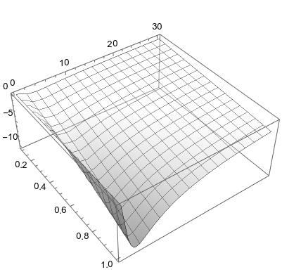
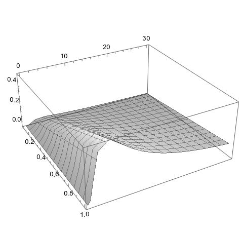
Figure 5: Discriminant $\Delta=\Delta(a\,,b)\leq 0\,$ (left) and coefficient $\,c_{5}=c_{5}(a\,,b)>0\,$ (right) for the quinticated form of oscillator (2) for $\,(a\,,b)\in]0\,,30]\times]0\,,1]\,$

The qualitative and quantitative behaviour of solution and period for the quinticated approximant to oscillator (2) is analogous to that seen in $\,\S$ 3 for the quinticated relativistic oscillator. The period ratio stays close to $1\,,$ as shown in Figure 6 (left). As for the differential operator (35), results were obtained with parameters $\,a>0\,$ and $\,0<b\leq 1\,$ and are not reported here, since they show precisely the same behaviour and equal order of magnitude as those synthetised in Figure 3 and Table1 for the case of the relativistic oscillator.

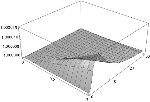
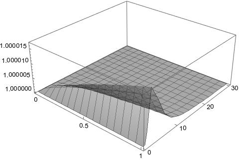
Figure 6: Period ratio in the case of the quinticated form of oscillator (2) (left) and oscillator (3) (right)

4.2 Duffing relativistic oscillator (3)

The normalised IVP, in this case, is:

$$\begin{cases}\ddot{u}=-u-a^{2}\;u^{3}-\dfrac{b\;u}{\sqrt{1+a^{2}\;\;u^{2}}}\;,\\ u(0)=1\,,\quad\dot{u}(0)=0\;,\end{cases}$$ (41)

thus function $\,\Phi(u)\,,$ defined in (5), becomes:

$$\Phi(u)=\dfrac{1}{2}\;(1-u^{2})\;(2+a^{2}+a^{2}\;u^{2})+\dfrac{2\,b}{a^{2}}\,\Big{(}\sqrt{1+a^{2}}-\sqrt{1+a^{2}\;u^{2}}\Big{)}\,,$$ (42)

so that forming $\,\Psi(u)\,$ as in (7) requires $\,4\,b>(2+a^{2}+a^{2}\,u^{2})\;(\sqrt{1+a^{2}}-\sqrt{1+a^{2}\,u^{2}})>0\,,$ being $\,a>0\,$ and $\,0<u<1\,.$

Setting $\,\mathcal{C}=-2/\pi\;$ and exploiting formulae (34) and (40), we have:

$$\alpha_{1} =\phantom{111}\mathcal{C}\;\left(w_{2}+a^{2}\;w_{4}+b\;J_{2}(a)\right)\;,$$ (43)

$$\alpha_{3} =-3\,\mathcal{C}\,\Big{(}w_{2}+a^{2}\,w_{4}+b\,J_{2}(a)\Big{)}+4\,\mathcal{C}\,\Big{(}w_{4}+a^{2}\,w_{6}+b\,J_{4}(a)\Big{)}$$

$$\alpha_{5} =\phantom{-}5\,\mathcal{C}\,\Big{(}w_{2}+a^{2}\,w_{4}+b\,J_{2}(a)\Big{)}-20\,\mathcal{C}\,\Big{(}w_{4}+a^{2}\,w_{6}+b\,J_{4}(a)\Big{)}+16\,\mathcal{C}\,\Big{(}w_{6}+a^{2}\,w_{8}+b\,J_{6}(a)\Big{)}\,,$$

on which $c_{1}=-(\alpha_{1}-3\,\alpha_{3}+5\,\alpha_{5})\;,\;c_{3}=-4\;(\alpha_{3}-5\,\alpha_{5})\;$ and $c_{5}=-16\;\alpha_{5}\;$ are build, as usual.

Figure 7 depicts discriminant $\,\Delta=\Delta(a\,,b)\,$ for varying $\,a\,,b>0\,,$ and shows how the values of $\,a\,$ and $\,b\,$ that satisfy either condition (i) or (ii) of (16) are closely related. As an example, it is $\,\Delta(a\,,0.5)\leq 0\,$ and $\,c_{5}(a\,,0.5)>0\,$ for $\,a\lessapprox 0.95\,;$ similarly, $\,\Delta(a\,,1)\leq 0\,$ and $\,c_{5}(a\,,1)>0\,$ for $\,a\lessapprox 1.7\,;$ therefore, in both of these cases, Theorem 2.1 applies. In particular, condition (i) starts being significantly verified when $\,b\geq 0.4\,,$ where $\,b\approx 0.4\,$ requires $a\lessapprox 0.7\,.$ Conversely, for $\,b\lessapprox 0.4\,$ and any $\,a\,,$ condition (ii) is verified and Theorem 2.2 comes into play.

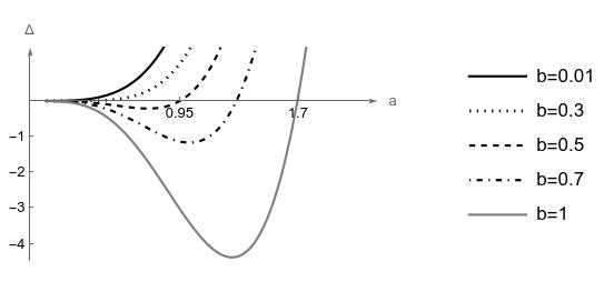
Figure 7: Discriminant $\Delta=\Delta(a\,,b)\,$ for the quinticated form of oscillator (3) for various couples $\,(a\,,b)\,$

The qualitative and quantitative behaviour of solution and period for the quinticated approximant to oscillator (3) is analogous as those commented in $\,\S$ 3 and $\,\S$ 4.1. The period ratio stays close to $1\,,$ as shown in Figure 6 (right). As for the differential operator (35), Figure 8 and Table2 report results achieved with couples $\,(a\,,b)\,$ requiring the solution $\,u\,$ given by Theorem 2.1, while Figure 9 and Table3 present the outcome related to couples $\,(a\,,b)\,$ for which the $\,u\,$ defined in Theorem 2.2 must be used; in both cases, we attain the same behaviour and equal, or improved, order of magnitude as in the previously studied quinticated forms of oscillators (1) and (2).

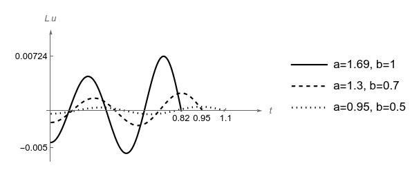
Figure 8: $\,L\,u\,,$ where $\,u\,$ is solution (19) with coefficients build on (43), for the quinticated form of oscillator (3)

a	0.95	1.3	1.69
b	0.5	0.7	1
$\|L\,u\|_{\infty}$	0.000487249	0.00229373	0.00724625

Table 2: Uniform norm of $\,L\,u\,,$ with $\,u\,$ solution (19) and coefficients build on (43), for the quinticated form of oscillator (3)

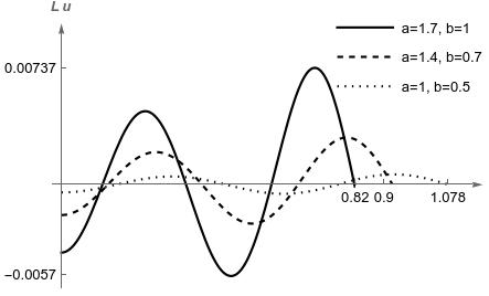
Figure 9: $\,L\,u\,,$ where $\,u\,$ is solution (25) with coefficients build on (43), for the quinticated form of oscillator (3)

a	1	1.4	1.7
b	0.5	0.7	1
$\|L\,u\|_{\infty}$	0.00064411	0.00298016	0.00737777

Table 3: Uniform norm of $\,L\,u\,,$ with $\,u\,$ solution (25) and coefficients build on (43), for the quinticated form of oscillator (3)

5 Conclusions

In this work we exploite Čebyšëv’s fifth-order approximations by applying them to three popular nonlinear oscillator models, which share the fact that the integrals obtained in the projection are expressible in closed form by means of complete elliptic integrals of the first and second kind. The approximate systems obtained, which by their nature constitute very good approximations of the considered models, are in turn explicitly solved in terms of Jacobian elliptic functions, which describe their cosine behaviour. The quality of the approximations obtained is confirmed in terms of the norm of the deviation of the solution, and in terms of the ratio between the periods of the approximating systems and the periods of the non-approximate systems solutions, which are however, in two cases out of three, expressible via complete elliptic integrals. All simulations are performed within the Mathematica scientific environment.

Financial disclosure

This research received no external funding.

Author contributions

The Authors share the content of this work, which is unpublished and has not been submitted to other journals. All Authors contributed equally to this work.

Conflict of interest

The Authors declare no conflict of interests.

References

- [1] L. MacColl, Theory of the relativistic oscillator, American J Physics 25 (8) (1957) 535–538. doi:10.1119/1.1934543.
- [2] R. Mickens, Periodic solutions of the relativistic harmonic oscillator, J Sound and Vibration 212 (5) (1998) 905–908.
- [3] D. Younesian, H. Askari, Z. Saadatnia, M. KalamiYazdi, Analytical approximate solutions for the generalized nonlinear oscillator, Applicable Analysis 91 (5) (2012) 965–977.
- [4] W. Sun, B. Wu, C. Lim, Approximate analytical solutions for oscillation of a mass attached to a stretched elastic wire, J Sound and vibration 300 (3–5) (2007) 1042–1047.
- [5] R. Mickens, Mathematical and numerical study of the duffing–harmonic oscillator, J Sound and Vibration 244 (3) (2001) 563–567.
- [6] D. Van Hieu, A new approximate solution for a generalized nonlinear oscillator, International J Applied and Computational Mathematics 5 (5) (2019) 1–13.
- [7] M. Razzak, An analytical approximate technique for solving cubic–quintic duffing oscillator, Alexandria Engineering J 55 (3) (2016) 2959–2965.
- [8] A. Beléndez, E. Arribas, T. Beléndez, C. Pascual, E. Gimeno, M. Álvarez, Closed–form exact solutions for the unforced quintic nonlinear oscillator, Advances in Mathematical Physics 2017 (2017).
- [9] A. Beléndez, T. Beléndez, F. Martinez, C. Pascual, M. Alvarez, E. Arribas, Exact solution for the unforced duffing oscillator with cubic and quintic nonlinearities, Nonlinear Dynamics 86 (3) (2016) 1687–1700.
- [10] M. Citterio, R. Talamo, The elliptic core of nonlinear oscillators, Meccanica 44 (6) (2009) 653.
- [11] A. Elias-Zuniga, Exact solution of the cubic–quintic duffing oscillator, Applied Mathematical Modelling 37 (4) (2013) 2574–2579.
- [12] G. Mingari Scarpello, D. Ritelli, Exact solution to a first–fifth power nonlinear unforced oscillator, Applied Mathematical Sciences 4 (69–72) (2010) 3589–3594.
- [13] R. Jonckheere, Determination of the period of nonlinear oscillations by means of chebyshev polynomials, Zeitschrift fur angewandte Mathematik und Mechanik 51 (5) (1971) 389–393.
- [14] A. Elias-Zuniga, Quintication method to obtain approximate analytical solutions of non–linear oscillators, Applied Mathematics and Computation 243 (2014) 849–855.
- [15] A. Big-Alabo, Approximate period for large–amplitude oscillations of a simple pendulum based on quintication of the restoring force, European Journal of Physics 41 (1) (2019) 015001.
- [16] A. Beléndez, D. Méndez, M. Alvarez, C. Pascual, T. Beléndez, Approximate analytical solutions for the relativistic oscillator using a linearized harmonic balance method, International J Modern Physics B 23 (04) (2009) 521–536.
- [17] J. Biazar, M. Hosami, An easy trick to a periodic solution of relativistic harmonic oscillator, J Egyptian Mathematical Society 22 (1) (2014) 45–49.
- [18] M. Hosen, M. Chowdhury, M. Ali, A. Ismail, A novel analytical approximation technique for highly nonlinear oscillators based on the energy balance method, Results in Physics 6 (2016) 496–504.
- [19] A. Nayfeh, Perturbation Methods, Wiley & Sons, New York, USA, 1973.
- [20] A. Nayfeh, D. Mook, Nonlinear oscillations, John Wiley & Sons, New York, USA, 1979.
- [21] R. Mickens, Oscillations in planar dynamic systems, World Scientific, Singapore, 1996.
- [22] N. Krylov, N. Bogoliubov, Introduction to non–linear mechanics, Princeton University Press, Princeton, NJ, USA, 1949.
- [23] J. He, Preliminary report on the energy balance for nonlinear oscillations, Mechanics Research Communications 29 (2–3) (2002) 107–111.
- [24] A. Beléndez, T. Beléndez, A. Márquez, C. Neipp, Application of He’s homotopy perturbation method to conservative truly nonlinear oscillators, Chaos, Solitons & Fractals 37 (3) (2008) 770–780.
- [25] R. Mickens, Truly nonlinear oscillations: harmonic balance, parameter expansions, iteration, and averaging methods, World Scientific, Singapore, 2010.
- [26] H. Gottlieb, Harmonic balance approach to periodic solutions of non–linear jerk equations, J Sound and Vibration 271 (3–5) (2004) 671–683.
- [27] H. Gottlieb, Harmonic balance approach to limit cycles for nonlinear jerk equations, J Sound and Vibration 297 (1–2) (2006) 243–250.
- [28] B. Wu, C. Lim, W. Sun, Improved harmonic balance approach to periodic solutions of non–linear jerk equations, Physics Letters A 354 (1–2) (2006) 95–100.
- [29] A. Beléndez, D. Méndez, T. Beléndez, A. Hernández, M. Alvarez, Harmonic balance approaches to the nonlinear oscillators in which the restoring force is inversely proportional to the dependent variable, J Sound and Vibration 314 (3–5) (2008) 775–782.
- [30] I. Kovacic, M. Brennan, The Duffing equation: nonlinear oscillators and their behaviour, John Wiley & Sons, New York, USA, 2011.
- [31] L. Cvetićanin, Strong Nonlinear Oscillators, Springer, Cham, Switzerland, 2014.
- [32] F. Rothe, The periods of the volterra–lotka system, J Reine Angew. Math 355 (1985) 129–138.
- [33] S. Foschi, G. Mingari Scarpello, D. Ritelli, Higher order approximation of the period–energy function for single degree of freedom hamiltonian systems, Meccanica 39 (4) (2004) 357–368.
- [34] R. Azami, D. Ganji, H. Babazadeh, A. Dvavodi, S. Ganji, He’s max–min method for the relativistic oscillator and high order duffing equation, International J Modern Physics B 23 (32) (2009) 5915–5927.
- [35] A. Beléndez, C. Pascual, E. Fernández, C. Neipp, T. Beléndez, Higher–order approximate solutions to the relativistic and duffing–harmonic oscillators by modified He’s homotopy methods, Physica Scripta 77 (2) (2008) 025004.
- [36] N. Jamshidi, D. Ganji, Application of energy balance method and variational iteration method to an oscillation of a mass attached to a stretched elastic wire, Current Applied Physics 10 (2) (2010) 484–486.
- [37] L. Zhao, He’s frequency–amplitude formulation for nonlinear oscillators with an irrational force, Computers & Mathematics with Applications 58 (11–12) (2009) 2477–2479.
- [38] A. Beléndez, A. Hernández, T. Beléndez, M. Alvarez, S. Gallego, M. Ortuno, C. Neipp, Application of the harmonic balance method to a nonlinear oscillator typified by a mass attached to a stretched wire, J Sound and Vibration 302 (4–5) (2007) 1018–1029.
- [39] J. Marion, Classical dynamics of particles and systems, Academic Press, New York, USA, 2013.
- [40] R. Graham, D. Knuth, O. Parashnik, Concrete Mathematics, 2nd ed., Addison–Wesley, Reading, MASS, USA, 1994.
- [41] L. Trefethen, Approximation Theory and Approximation Practice, SIAM, Philadelphia, PA, USA, 2019.
- [42] G. Phillips, P. Taylor, Theory and Applications of Numerical Analysis, 2nd ed., Academic Press, Elsevier Science Technology, Boston, MASS, USA, 1996.
- [43] A. Beléndez, M. Alvarez, J. Francés, S. Bleda, T. Beléndez, A. Nájera, E. Arribas, Analytical approximate solutions for the cubic–quintic duffing oscillator in terms of elementary functions, J Applied Mathematics Volume 2012, Article ID 286290 (2012).
- [44] A. Beléndez, A. Hernandez, T. Beléndez, C. Pascual, , M. Alvarez, E. Arribas, Solutions for conservative nonlinear oscillators using an approximate method based on chebyshev series expansion of the restoring force, ACTA PHYSICA POLONICA A 130 (3) (2016) 667–678.
- [45] H. Khalil, M. Khalil, I. Hashim, P. Agarwal, Extension of operational matrix technique for the solution of nonlinear system of caputo fractional differential equations subjected to integral type boundary constrains, Entropy 29 (3) (2021) 1154.
- [46] I. Gradshteyn, J. Ryzhik, Table of Integrals, Series and Products 6th ed, Academic Press, New York, USA, 2000.
- [47] P. Byrd, M. Friedman, Handbook of elliptic integrals for engineers and scientists, Springer Berlin, New York, USA, 1971.
- [48] S. Wolfram, An Elementary Introduction to the Wolfram Language, 2nd ed., Wolfram Media, Inc., Urbana–Champaign, ILL, USA, 2017.