Energy limit of compact isochronous cyclotrons

Abstract

Existing analytical models for transverse beam dynamics in isochronous cyclotrons are often not valid or not precise for relativistic energies. The main difficulty in developing such models lies in the fact that cross-terms between derivatives of the average magnetic field and the azimuthally varying components cannot be neglected at higher energies. Taking such cross-terms rigorously into account results in an even larger number of terms that need to be included in the equations. In this paper, a method is developed which is relativistically correct and which provides results that are practical and easy to use. We derive new formulas, graphs and tables for the radial and vertical tunes in terms of the the flutter, its radial derivatives, the spiral angle and the relativistic gamma. Using this method, we study the $2\nu_{r}=N$ structural resonance ($N$ is number of sectors) and provide formulas and graphs for its stopband and for the modified radial tune. Combining those equations with the new equation for the verical tune, we find the stability zone and the energy limit of compact isochronous cyclotrons for any value of N. We confront the new analytical method with closed orbit simulations of the IBA C400 cyclotron for hadron therapy.

1 Introduction

In this paper we derive the maximum energy that can be realized in compact isohronous cyclotrons. This limit is determined by two competing requirements namely the need for sufficient vertical focusing on the one hand and the need to avoid the stopband of the half-integer resonance $2\nu_{r}=N$ on the other hand ($N$ is the cyclotron rotational symmetry number; $\nu_{r}$ is the radial tune). With increasing energy the isochronous field index $\bar{\mu}^{\prime}$ increases rapidly and more and more azimuthal field variation $f$ is needed to remain vertically stable; but with higher $f$, the stopband of the resonance broadens and the energy limit associated with it rapidly reduces. The energy limit depends on $N$ and on the spiral angle $\xi$ of the sectors. We derive practical formulas which are useful especially in the design phase of a new cyclotron. Our main assumption/approximation is that $f$ is not too large. Results are derived up to $\mathscr{O}(f^{2})$ (equivalent to $\mathscr{O}(F)$, where $F$ is the flutter). For compact cyclotrons $F$ is generally well below $1$ and for these machines we expect our results to be precise. For seperate sector cyclotrons, care should be taken however. The special case of such cyclotrons with radial sectors (no spiraling) has been studied by Gordon[1], by assuming a hard-edge model where in the magnet sections the orbits are perfectly circular and in the empty straight sections the magnetic field is zero. In Gordon’s model, there is no need to assume a small flutter, but on the other hand his assumptions will probably not be valid for compact cyclotrons and maybe also less accurate for coil-dominated superconducting ring cyclotrons where the magnetic field has the tendency to spread out more smoothly and non-uniformly. For seperate sector cyclotrons with a larger magnetic filling factor the flutter drops quickly ($F\approx 0.25$ for a filling factor of 80%) and we expect our results to become more accurate. Another interesting derivation of the isochronous cyclotron energy limit has been made by Danilov et al. from the JINR[2]. In their analysis however, they take into account only the first dominant Fourier component of the field and they further assume that its amplitude is independent on radius and its phase increases linearly with radius. Also contributions due to higher order radial derivatives of the average magnetic field are ignored. We closely follow the Hamiltonian approach that has been firstly introduced by Hagedoorn and Verster[3]; in this paper we wish to pay tribute to them.

2 Method of derivation

We study the static (non-accelerated) motion near a given radius $r_{0}$ which is related to the constant kinetic momentum $P_{0}$ of a particle. The reduced magnetic field $\mu(r,\theta)$ around this radius is represented by a Fourier series with respect to the azimuth $\theta$ and the radial dependence of the average field $\bar{\mu}(r)$ and the normalized Fourier coefficients $A_{n}(r),B_{n}(r)$ are Taylor expanded relative to the same radius $r_{0}$. The magnitude of azimuthal field variation $f$ is approximately equal to the magnitude of the dominant Fourier component $C_{N}=(A_{N}^{2}+B_{N}^{2})^{1/2}$ and the flutter $F$ is approximately equal to $C_{N}^{2}/2$. We develop the general Hamiltonian $H_{0}$ in polar coordinates relative to the circle $r_{0}$ and first look for the closed orbit (CO) which is the $N$-fold rotational symmetric solution of $H_{0}$. In all our derivations we use a pertubation analysis where $|f|$ serves as the measure for precission. In general any quantity of interest $g(\theta)$ can be split in its average part $\bar{g}=\tfrac{1}{2\pi}\oint g(\theta)d\theta$ and its oscillating part $osc(g)=g(\theta)-\bar{g}$. Oscillating parts of $\mathscr{O}(f)$ can be moved to the next higher order by a properly constructed canonical transformation. In doing so, new average contributions of $\mathscr{O}(f^{2})$ are generated. Our goal is to derive results up to $\mathscr{O}(f)$. The reason for this is that the first significant terms in the expressions for the isochronous magnetic field and the radial and vertical tunes are of $\mathscr{O}(f^{2})$. In line with the HV-paper[3], we keep the average part of any azimuthally varying term up to $\mathscr{O}(f^{2})$, but neglect oscillating terms $\mathscr{O}(f^{2})$ as they would generate new terms of $\mathscr{O}(f^{3})$ when transforming them to higher order. However, we make one important generalization/improvement as compared to the HV-paper. In their analysis Hagedoorn and Verster assumed that radial derivatives of the average magnetic field ($\bar{\mu}^{\prime},\bar{\mu}^{\prime\prime},\bar{\mu}^{\prime\prime\prime},\dots$) are small quantities of $\mathscr{O}(f^{2})$ and therefore neglect cross-terms between those derivatives and the Fourier content of the magnetic field in all expansions. This is a valid approach at lower energies where the radial isochronous field derivatives are still small, but at higher energies this approximation becomes less and less accurate and ultimately breaks down completely. Since we are interested in the higher-energy limits of the isochronous cyclotron we cannot make this concession and therefore keep those cross-terms. This makes the derivation and also the final results considerably more complex as many more terms need to be kept in the Hamiltonian expansion. The $\mathscr{O}(f^{2})$ contributions to the final results all have a similar structure of the following general form:

$$R^{(2)}=\sum_{n}\alpha_{n}(\bar{\mu}^{\prime},\dots)C_{n}^{2}+\beta_{n}(\bar{\mu}^{\prime},\dots)C_{n}^{2}\varphi_{n}^{\prime 2}+\gamma_{n}(\bar{\mu}^{\prime},\dots)C_{n}C_{n}^{\prime}+\delta_{n}(\bar{\mu}^{\prime},\dots)C_{n}^{\prime 2}\ .$$ (1)

Here the summation runs over all the Fourier components ($n=kN,\hskip 2.84544ptk=1,2,\dots$) present in the magnetic field; the coefficients $\alpha_{n},\dots$ depend on the first and higher radial derivatives $\bar{\mu}^{\prime},\bar{\mu}^{\prime\prime},\bar{\mu}^{\prime\prime\prime},\dots$ of the average magnetic field and the variable $\varphi^{\prime}_{n}$ is the radial derivative of the phase $\varphi_{n}$ of the Fourier harmonic $n$. To obtain practical results we make a few assumptions and approximations that allow us to simplify this structure. Firstly it is assumed that the magnetic field is perfectly isochronous. In this case the form-factor of the average field is completely determined by the relativistic gamma parameter and therefore the coefficients $\alpha_{n},\dots$ will depend on $\gamma$ only. Secondly we assume that the phase-derivatives $\varphi^{\prime}_{n}$ do not depend on $n$. In practice this is accurately true for the first several (often up to 5) Fourier components. Since contributions of higher components rapidly drop with increasing $n$-value, this approximation must be accurate. In this way the variable $\varphi^{\prime}_{n}=\varphi^{\prime}$ can be taken out of the series summations. Thirdly we introduce a method where the higher Fourier harmonics ($n>N$) are expressed in terms of the dominant harmonic ($n=N$). For this we assume a hard-edge profile of the azimuthally varying field with a symmetrical structure of equal hill and valley angle. For such a profile only the odd harmonics ($k=1,3,\dots$) are non-zero and the magnitude of the harmonics drop with $1/n$. In this way, the n-dependence of the harmonic amplitudes $C_{n}$ can be included in the coefficients $\alpha_{n},\dots$ and the dominant components $C_{N}$ can be taken outside of the series summation. The assumption of a hard-edge profile represents a certain limitation but it allows us to approximately take into account the higher harmonic content and therefore is expected to be better than just taking into account the dominant harmonic; at the same time it allows to express the dominant Fourier coefficients $C_{N}$ in terms of the flutter $F$. In a final step we sum the series analytically and express the results in elementary functions of $\gamma$ and $N$. The $\mathscr{O}(f^{2})$ contributions to the final results are thus transformed to the following simpler form:

$$R^{(2)}\approx F\left(a_{N}(\gamma)+b_{N}(\gamma)\varphi^{\prime 2}+c_{N}(\gamma)\frac{F^{\prime}}{F}+d_{N}(\gamma)(\frac{F^{\prime}}{F})^{2}\right)\ .$$ (2)

The above method is applied in the derivation of the isochronous magnetic field, the radial and vertical tunes and the stopband of the half-integer resonance.

3 The radial motion

The Hamiltonian for the radial motion with respect the reference circle $r_{0}$ (see Eq. (A14)) has been given in Eq. (A29). In this paragraph we derive the expressions for the equilibrium orbit (EO) and the isochronous magnetic field. We also determine the relation between the particle relativistic parameter $\gamma$ and the field index $\bar{\mu}^{\prime}$ and express the higher derivatives $\bar{\mu}^{\prime\prime},\bar{\mu}^{\prime\prime\prime}$ in terms of $\bar{\mu}^{\prime}$. We derive the Hamiltonian with respect to the EO and bring it into its normal form. Then we solve the linear motion giving us expressions for the radial tune $\nu_{r}$ and the stopband of the $2\nu_{r}=N$ resonance. In the analysis we keep oscillating terms of $\mathscr{O}(f^{1})$ but neglect those of higher order. Constant ($\theta$-independent) terms are are kept up to $\mathscr{O}(f^{2})$. Radial derivatives of the averge field such as $\bar{\mu}^{\prime},\bar{\mu}^{\prime\prime},\bar{\mu}^{\prime\prime\prime}$ are considered as terms of $\mathscr{O}(f^{0})$ and are always kept. In the final results, summations over magnetic field Fourier coefficients and their radial derivatives are eliminated and replaced by expressions with flutter and spiral angle. The derivatives of the average field are eliminated as they are considerd as functions of the relativistic parameter $\gamma$.

3.1 The equilibrium orbit

The EO is a closed orbit in the median plane with the same $N$-fold symmetry as the magnetic field. it can therefore can be expanded in a Fourier series:

$$x_{e}(\theta)=\gamma_{e}+\operatorname*{\textstyle\sum}_{n}\alpha_{n}\cos n\theta+\beta_{n}\sin n\theta\ .$$ (3)

We need to find the expressions for $\alpha_{n}$ and $\beta_{n}$ up to $\mathscr{O}(f)$ and the expression for $\gamma_{e}$ up to $\mathscr{O}(f)$. The radial equations of motion are obtained from Eq. (A29) as:

$$\frac{dx}{d\theta}\hskip 2.84544pt=\hskip 9.95863pt\frac{\partial H_{x}}{\partial p_{x}}=(1+x)p_{x}(1-p_{x}^{2})^{-1/2}\ ,$$

$$\frac{dp_{x}}{d\theta}=-\frac{\partial H_{x}}{\partial x}=(1-p_{x}^{2})^{1/2}-(1+x)\mu(\theta,x)\ .$$

Knowing that both $x$ and $p_{x}$ are functions of $\mathscr{O}(f)$ we can expand the right hand sides of above equations up to $\mathscr{O}(f^{2})$. From the first equation we will get:

$$\frac{dx}{d\theta}=(1+x)p_{x}=p_{x}+\mathscr{O}(f^{2})\ ,$$

because here we can neglect a term $xp_{x}$ as $\langle xp_{x}\rangle=0$. Inserting $\dot{p}_{x}=\ddot{x}$ and the expression for the reduced field $\mu$ from Eq. (B10) in the second equation, we get:

$$\ddot{x}= -\tfrac{1}{2}\dot{x}^{2}-(1+\bar{\mu}^{\prime})x-(\bar{\mu}^{\prime}+\tfrac{1}{2}\bar{\mu}^{\prime\prime})x^{2}$$

$$-\operatorname*{\textstyle\sum}_{n}\left[A_{n}+(A_{n}+A^{\prime}_{n})x\right]\cos n\theta+\left[B_{n}+(B_{n}+B^{\prime}_{n})x\right]\sin n\theta)\ .$$

Note that the “dot”-operator stands for differentiation with respect to $\theta$ ($\dot{x}=\tfrac{dx}{d\theta}$). In the expression above we insert the Fourier expansion of $x=x_{e}$ from Eq. (3). The first order parts of the equation give us the expressions for $\alpha_{n},\beta_{n}$. For the second order parts we only have to keep the average values. This gives us the expression for $\gamma_{e}$. We find for the Fourier coefficients of the EO:

$$\alpha_{n}=\frac{A_{n}}{n^{2}-1-\bar{\mu}^{\prime}}\ ,$$ (4)

$$\beta_{n}=\frac{B_{n}}{n^{2}-1-\bar{\mu}^{\prime}}\ ,$$ (5)

$$\gamma_{e}=-\frac{1}{2(1+\bar{\mu}^{\prime})}\sum_{n}\left[\frac{3n^{2}-2+\bar{\mu}^{\prime\prime}}{2(n^{2}-1-\bar{\mu}^{\prime})^{2}}C_{n}^{2}+\frac{C_{n}C^{\prime}_{n}}{n^{2}-1-\bar{\mu}^{\prime}}\right]\ .$$ (6)

In the expression for $\gamma_{e}$ we used Eqs. (B13,B14) to eliminate the sin/cosine coefficients $A_{n},B_{n}$ in favour of the Fourier amplitude $C_{n}$.

The radial momentum of the EO is given by $p_{e}=\dot{x}_{e}$.

3.2 Correction of the spiral angle

In paragraph B.3 we have defined the spiral angle as the angle between the tangent along the sector contour and the normal to the orbit. However, the EO is not exactly a circle as there is a small angle between the normal vector of the circle and the normal vector of the orbit. This angle is equal to the arc tangent of the radial momentum of the EO. We can therefore define a corrected spiral angle $\bar{\xi}$ as follows:

$$\bar{\xi}=\xi+\arctan(p_{e})=\arctan(\varphi^{\prime})+\arctan(p_{e})\ .$$

Here $\xi,\varphi^{\prime}$ are the uncorrected parameters. With $\bar{\varphi}^{\prime}=\tan(\bar{\xi})$ we get:

$$\bar{\varphi}^{\prime}=\frac{\varphi^{\prime}+p_{e}}{1-\varphi^{\prime}p_{e}}\ .$$

From paragraph (3.1) we have for $p_{e}$:

$$p_{e}(\theta)=\dot{x_{e}}=-\operatorname*{\textstyle\sum}_{n}\frac{nC_{n}}{n^{2}-1-\bar{\mu}^{\prime}}\sin n(\theta-\varphi_{n})\approx-\operatorname*{\textstyle\sum}_{n}\frac{C_{n}}{n}\sin n(\theta-\varphi_{n})\ .$$ (7)

We evaluate $p_{e}$ at the entrance (and exit) of the sector and assume (as we did in paragraph B.4) a symmetric structure where the hill angle is equal to the valley angle. In this case we get $\theta-\varphi_{n}\approx\theta-\varphi=\pm\pi/2N$ and then get (with $n=(2k+1)N$):

$$\sin n(\theta-\varphi_{n})\approx\pm(-1)^{k}\ ,$$

Inserting this expression in Eq. (7), together with the expressions for the Fourier components Eq. (B19) and the relation for the flutter Eq. (B24), we find the following approximation for the radial momentum at the sector edges:

$$p_{e}=\pm\frac{\pi}{2N}\sqrt{F}\ .$$

It is seen that the correction at the pole edges have opposite sign and we can take the average of the two as good approximation for the corrected paramater $\bar{\varphi^{\prime}}$:

$$\bar{\varphi}^{\prime}=\frac{1}{2}\left[\frac{\varphi^{\prime}_{in}+\frac{\pi}{2N}\sqrt{F}}{1-\frac{\pi}{2N}\varphi^{\prime}_{in}\sqrt{F}}+\frac{\varphi^{\prime}_{out}-\frac{\pi}{2N}\sqrt{F}}{1+\frac{\pi}{2N}\varphi^{\prime}_{out}\sqrt{F}}\right]\ .$$ (8)

We use Eq (8) in paragraph (vermot), when we compare the analytical expression of the vertical tune $\nu_{z}$ with results from closed orbit simulations for the IBA C400 cyclotron.

For cyclotron design studies one normaly will start with equal pole-edge contours at the sector entrance and exit. In this case one can take $\varphi^{\prime}_{in}=\varphi^{\prime}_{out}=\varphi^{\prime}$ and the expression for the corrected spiral simplifies to:

$$\boxed{\bar{\varphi}^{\prime}=\varphi^{\prime}_{geom}\left(1+\frac{\pi^{2}F}{4N^{2}}(1+\varphi^{\prime 2}_{geom})\right)+\mathscr{O}(f^{4})\ .}$$ (9)

Here $\varphi_{geom}$ represents the geometrical pole-edge contour.

3.3 The isochronous magnetic field

The shape of the isochronous magnetic field $B_{iso}(r)$ has been given in Eq. (5.5) of the HV-paper[3] as:

$$B_{iso}(r)=B_{0}\frac{R_{e}}{r_{0}}\left[1-\left(\frac{R_{e}}{\lambda}\right)^{2}\right]^{-1/2}\ ,$$ (10)

where $B_{0}=m_{0}\omega/q$ is the center magnetic field and $\omega$ is the (constant) angular revolution frequency of a particle (with restmass $m_{0}$ and charge $q$) and $\lambda=c/\omega$, with $c$ the speed of light. The radius $R_{e}$ is the effective radius of the EO and is defined as its length divided by $2\pi$:

$$R_{e}=\frac{1}{2\pi}\oint_{EO}ds=r_{0}\langle(1+x_{e})(1-p_{e}^{2})^{-1/2}\rangle\ .$$ (11)

We write:

$$R_{e}=r_{0}(1+\epsilon_{e})\ .$$ (12)

Up to $\mathscr{O}(f^{2})$ we find for $\epsilon_{e}$:

$$\epsilon_{e} =\langle x_{e}+\tfrac{1}{2}p_{e}^{2}\rangle=\gamma_{e}+\tfrac{1}{4}\sum_{n}\frac{n^{2}C_{n}^{2}}{(n^{2}-1-\bar{\mu}^{\prime})^{2}}\ ,$$ (13)

$$=-\frac{1}{2(1+\bar{\mu}^{\prime})}\sum_{n}\left[\frac{2(n^{2}-1)-n^{2}\bar{\mu}^{\prime}+\bar{\mu}^{\prime\prime}}{2(n^{2}-1-\bar{\mu}^{\prime})^{2}}C_{n}^{2}+\frac{C_{n}C^{\prime}_{n}}{n^{2}-1-\bar{\mu}^{\prime}}\right]\ ,$$

and for $B_{iso}(r)$:

$$B_{iso}(r)=\frac{B_{0}}{\sqrt{1-r^{2}/\lambda^{2}}}\left(1+\frac{\epsilon_{e}}{1-r^{2}/\lambda^{2}}\right)\ .$$ (14)

We also calculate the field-index $\bar{\mu}^{\prime}_{iso}$ of the iscochronous field and find:

$$\bar{\mu}^{\prime}_{iso}=\frac{r}{B_{iso}}\frac{dB_{iso}}{dr}=\frac{r^{2}/\lambda^{2}}{1-r^{2}/\lambda^{2}}\left[1+\frac{2\epsilon_{e}}{1-r^{2}/\lambda^{2}}+\frac{\lambda^{2}}{r^{2}}\epsilon^{\prime}_{e}\right]\ ,$$ (15)

where $\epsilon^{\prime}_{e}=rd\epsilon_{e}/dr$.

We now look for a relation between the field index and the relativistic parameter $\gamma$. For this we use the definition of our reference momentum $P_{0}$ from eq. (A14) which now is applied for the isochronous field Eq. (14):

$$\frac{P_{0}}{m_{0}c}=\beta\gamma=\frac{qrB_{iso}(r)}{m_{0}c}=\frac{r/\lambda}{\sqrt{1-r^{2}/\lambda^{2}}}\left(1+\frac{\epsilon}{1-r^{2}/\lambda^{2}}\right)\ .$$ (16)

from which we get:

$$\gamma^{2}-1=\frac{r^{2}/\lambda^{2}}{1-r^{2}/\lambda^{2}}\left[1+\frac{2\epsilon_{e}}{1-r^{2}/\lambda^{2}}\right]\ .$$ (17)

Comparing the right hand side of this equation with the right hand side of Eq. (15), we can write $\bar{\mu}^{\prime}_{iso}$ as follows:

$$\bar{\mu}^{\prime}_{iso}=\gamma^{2}-1+\gamma^{2}\epsilon^{\prime}_{e}.\ .$$ (18)

So, since we assume that the magnetic field is iscochronous, we can split the field index $\bar{\mu}^{\prime}=\bar{\mu}^{\prime}_{iso}$ in a relativistic part and a flutter part as follows:

$$\bar{\mu}^{\prime}=\bar{\mu}^{\prime}_{rel}+\bar{\mu}^{\prime}_{fl}\ ,$$ (19)

$$\bar{\mu}^{\prime}_{rel}=\gamma^{2}-1\ ,$$ (20)

$$\bar{\mu}^{\prime}_{fl}=(1+\bar{\mu}^{\prime})\epsilon^{\prime}_{e}\ .$$ (21)

We further note that, in expressions which are already of $\mathscr{O}(f^{2})$ (such as the expression for $\gamma_{e}$ in Eq. (6), the expression for $\epsilon_{e}$ in Eq. (13) and also in the expression on the right hand side of Eq. (20)), we can ignore the difference between $\bar{\mu}^{\prime}$ and $\bar{\mu}^{\prime}_{rel}$ since the difference will generate terms of $\mathscr{O}(f^{4})$. For the same reason we can, for such expressions, calculate the higher derivatives of the average field $\bar{\mu}^{\prime\prime},\bar{\mu}^{\prime\prime\prime},\dots$ by differentiation of the function $b(r)=b_{0}/\sqrt{1-r^{2}/\lambda^{2}}$. In this way the higher derivatives can expressed in $\bar{\mu}^{\prime}$. We find in this way:

$$\bar{\mu}^{\prime\prime}=\bar{\mu}^{\prime}(1+3\bar{\mu}^{\prime})+\mathscr{O}(f^{2})\ ,$$ (22)

$$\bar{\mu}^{\prime\prime\prime}=3\bar{\mu}^{\prime 2}(3+5\bar{\mu}^{\prime})+\mathscr{O}(f^{2})\ .$$ (23)

Figure 1 shows the (relativistic part) of the field-derivitatives $\bar{\mu}^{\prime},\bar{\mu}^{\prime\prime}$ and $\bar{\mu}^{\prime\prime\prime}$. It is seen that especially the second and third derivatives become large for relativistic energies.

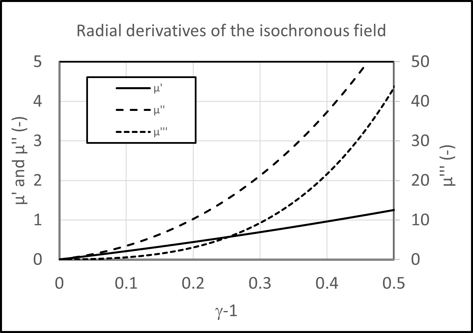
Figure 1: Normalized first and second derivatives (left scale) and third derivative (right scale) of an isochronous magnetic field.

In paragraphs 3.4 and 4, where we derive the radial and vertical tunes, we need to make the split $\bar{\mu}^{\prime}=\bar{\mu}^{\prime}_{rel}+\bar{\mu}^{\prime}_{fl}$, as we want to combine the term $\bar{\mu}^{\prime}_{fl}$ with other contributions arising from the azimuthally varying part of the magnetic field. For that we need to calculate the expression for $\bar{\mu}^{\prime}_{fl}$. We find this by differentiation and by carefully taking into account all radius-dependent terms ($\bar{\mu}^{\prime},\bar{\mu}^{\prime\prime},C_{n},C_{n}^{\prime}$) in Eqs. (20) and (13). For the radial derivatives of $\bar{\mu}^{\prime},\bar{\mu}^{\prime\prime},C_{n}^{\prime}$ we have:

$$r\frac{d}{dr}C^{\prime}_{n}=C^{\prime}_{n}+C^{\prime\prime}_{n}\ ,$$ (24)

$$r\frac{d}{dr}\bar{\mu}^{\prime}=\bar{\mu}^{\prime}-\bar{\mu}^{\prime 2}+\bar{\mu}^{\prime\prime}=2\bar{\mu}^{\prime}(1+\bar{\mu}^{\prime})\ ,$$ (25)

$$r\frac{d}{dr}\bar{\mu}^{\prime\prime}=r\frac{d}{dr}[\bar{\mu}^{\prime}(1+3\bar{\mu}^{\prime})]=2\bar{\mu}^{\prime}(1+\bar{\mu}^{\prime})(1+6\bar{\mu}^{\prime})\ .$$ (26)

Using these expressions we find for $\bar{\mu}^{\prime}_{fl}$:

$$\bar{\mu}^{\prime}_{fl} =\operatorname*{\textstyle\sum}_{n}\frac{-1}{2(n^{2}-1-\bar{\mu}^{\prime})}{{{\{}}}\frac{-\bar{\mu}^{\prime}\left[(n^{2}-1)\left(3n^{2}-7-\bar{\mu}^{\prime}(11+\bar{\mu}^{\prime})\right)-3\bar{\mu}^{\prime 3}\right]}{(n^{2}-1-\bar{\mu}^{\prime})^{2}}C_{n}^{2}$$

$$+\frac{\left[3(n^{2}-1)-3\bar{\mu}^{\prime}n^{2}+4\bar{\mu}^{\prime}+7\bar{\mu}^{\prime 2}\right]}{n^{2}-1-\bar{\mu}^{\prime}}C_{n}C^{\prime}_{n}+C_{n}C^{\prime\prime}_{n}+C^{\prime 2}_{n}{{{\}}}}$$ (27)

We now further elaborate on the expression for $\epsilon_{e}$ given in Eq. (13) as this term is needed to calculate the precise expression for the isochronous field $B_{iso}$ (given in Eq. (14)) and for obtaining a precise relation between radius $r$ and $\gamma$ as determined by the relation Eq. (17). We insert $\bar{\mu}^{\prime\prime}=\bar{\mu}^{\prime}(1+3\bar{\mu}^{\prime})$ (see Eq. (22)) in the expression for $\epsilon_{e}$ and then simplify this expression by the method explained in paragraph B.4 where we substitute for the Fourier coefficient $C_{n}$ their expressions in terms of the flutter $F$ as defined in Eqs. (LABEL:CtoF).

The result for $\epsilon_{e}$ can now be written as follows:

$$\boxed{\epsilon_{e}=-\frac{F}{2\gamma^{4}}\left(\check{a}_{N}+\check{c}_{N}\frac{F^{\prime}}{F}\right)\ .}$$ (28)

Here $F$ is the flutter and $F^{\prime}$ its radial derivative. The functions $\check{a}_{N},\check{c}_{N}$ depend only on the symmetry number $N$ and on the relativistic parameter $\gamma$ via the relation $\bar{\mu}^{\prime}=\bar{\mu}^{\prime}_{rel}=\gamma^{2}-1$. The expressions for these parameters are obtained as:

$$\check{a}_{N} =\frac{8\gamma^{2}N^{2}}{\pi^{2}}\sum_{k=0}\frac{2-\bar{\mu}^{\prime}}{(n^{2}-1-\bar{\mu}^{\prime})^{2}}+\frac{-2+\bar{\mu}^{\prime}+3\bar{\mu}^{\prime 2}}{n^{2}(n^{2}-1-\bar{\mu}^{\prime})^{2}}\ ,$$ (29)

$$\check{c}_{N} =\frac{8\gamma^{2}N^{2}}{\pi^{2}}\sum_{k=0}\frac{1}{n^{2}(n^{2}-1-\bar{\mu}^{\prime})^{2}}\ .$$ (30)

In these equations we have to replace $n$ by $n=(2k+1)N$.

The summations in the above equations can be done analytically and the coefficients $\check{a}_{N},\check{c}_{N}$ can be expressed in elementary mathematical functions. Appendix E shows how this is done. We find the following result:

$$\check{a}_{N} =(4\gamma^{2}-6)\left[1-\frac{2N}{\pi\gamma}\tan(\frac{\pi\gamma}{2N})\right]+(\gamma^{2}-1)\tan^{2}(\frac{\pi\gamma}{2N})\ ,$$ (31)

$$\check{c}_{N} =-1+\frac{2N}{\pi\gamma}\tan(\frac{\pi\gamma}{2N})\ .$$ (32)

One can now obtain the isochronous field as function of radius from Eq. (14) and the relation between $\gamma$ and radius $r$ from Eq. (17), where $\epsilon_{e}$ is calculated from Eq. (28). We re-arrange the equations as follows:

$$\gamma_{0}\hskip 22.76228pt=1/\sqrt{1-r^{2}/\lambda^{2}}\ ,$$ (33)

$$\gamma\hskip 28.45274pt=\gamma_{0}{{[}}1-\frac{\gamma_{0}^{2}-1}{2\gamma_{0}^{4}}{{(}}\check{a}_{N}F+\check{c}_{N}F^{\prime}{{)}}{{]}}+\mathscr{O}(f^{4})\ ,$$ (34)

$$B_{iso}(r)=B_{0}\gamma_{0}{{[}}1-\frac{1}{2\gamma_{0}^{2}}{{(}}\check{a}_{N}F+\check{c}_{N}F^{\prime}{{)}}{{]}}+\mathscr{O}(f^{4})\ .$$ (35)

Here $\gamma_{0}$ is the $\mathscr{O}(f^{0})$ solution for $\gamma$ and the coefficients $\check{a}_{N},\check{c}_{N}$ must be evaluated at $\gamma=\gamma_{0}$.

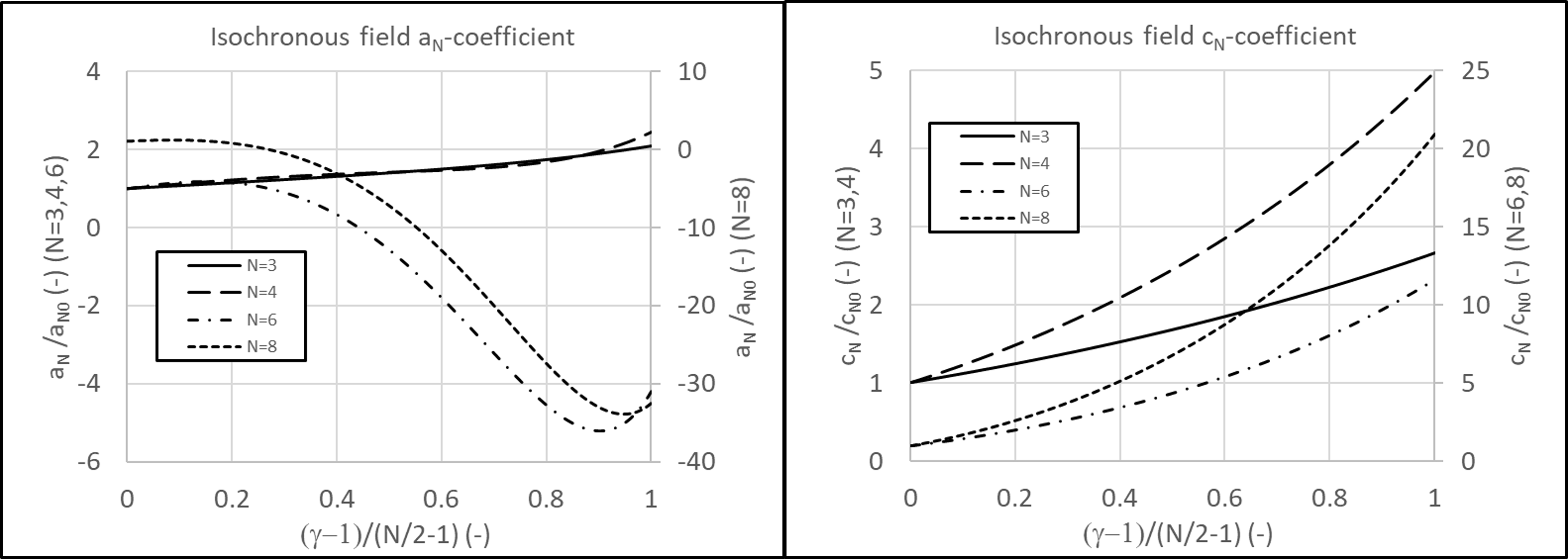
Figure 2: Energy dependence of the isochronous field coefficients.

Figure 2 shows the energy dependence of the isochronous field coefficients $\check{a}_{N},\check{c}_{N}$ . The horizontal axis represents the relativistic kinetic energy $\gamma-1$, normalized by the factor $\tfrac{N}{2}-1$, i.e. the energy at which the half-integer resonance is hit (in case the stopband width equals zero, i.e. when there would be no azimuthal field variation). This representation will be used several times in this report. The highest scale value of 1.0 as used in Figure 2 therefore represents 100% of the “N/2 band-width”. The vertical scale is normalized with respect to the coefficients-value at zero kinetic energy ($\gamma=1$). It is seen from Figure 2 that the coefficient $\check{a}_{N}$ becomes large and negative, for high N-numbers. For such cases the required increase of the isochronous field may be under-estimated at large energies.

3.4 The linear radial motion

We study the linear radial motion around the EO and for this purpose introduce new canonical variables $(\pi,\xi)$ which eliminate the EO from the motion. The method has been described in paragraph G.3 and the transformation is:

$$\pi =p_{x}-p_{e}\ ,$$ (36)

$$\xi =x-x_{e}\ ,$$

The new Hamiltonian $K_{x}$ is obtained as a Taylor expansion around $x_{e},p_{e}$ (and with respect to $\pi$ and $\xi$) of the Hamiltonian $H_{x}$ given in Eq. (A29). For the linear motion we only have to keep terms up to second degree in $\pi$ and $\xi$. In their coefficients we have to keep constants up to $\mathscr{O}(f^{2})$ and oscillating terms up to $\mathscr{O}(f)$. We obtain:

$$K_{x}(\xi,\pi,\theta)=\tfrac{1}{2}\left(1+x_{e}+\tfrac{3}{2}\dot{x}_{e}^{2}\right)\pi^{2}+\dot{x}_{e}\pi\xi+\tfrac{1}{2}\left(\mu+(1+x_{e})\frac{\partial\mu}{\partial x}\right)\xi^{2}\ .$$ (37)

This expression agrees with Eq. (6.3) in the HV-paper. Note that here, we have to evaluate $\mu$ and $\frac{\partial\mu}{\partial x}$ on the EO (so at $x=x_{e}$). We bring this Hamiltonian to its normal form by a canonical transformation $\pi,\xi\Rightarrow P_{x},X$ using the method explained in paragraph G.4. This gives us for the new Hamiltonian $\bar{K}_{x}(X,P_{x})$:

$$\bar{K}_{x}(X,P_{x})=\tfrac{1}{2}P_{x}^{2}+\tfrac{1}{2}Q_{x}(\theta)X^{2}\ ,$$ (38)

where $Q_{x}(\theta)$ is given by:

$$Q_{x}(\theta)=\mu+\frac{\partial\mu}{\partial x}-\tfrac{1}{2}\ddot{x}_{e}+x_{e}(\mu+2\frac{\partial\mu}{\partial x})+\frac{\partial\mu}{\partial x}x_{e}^{2}+(-\tfrac{1}{4}+\tfrac{3}{2}\mu+\tfrac{3}{2}\frac{\partial\mu}{\partial x})\dot{x}_{e}^{2}\ .$$ (39)

We calculate the partial derivative $\partial\mu/\partial x$ from the expression for the reduced field $\mu$ given in Eq. (B10) and insert it together with the expression for $\mu$ in Eq. (39). With this we obtain:

$$Q_{x}(\theta) =1+\bar{\mu}^{\prime}$$

$$+(1+3\bar{\mu}^{\prime}+\bar{\mu}^{\prime\prime})x_{e}+\tfrac{1}{2}(4\bar{\mu}^{\prime}+5\bar{\mu}^{\prime\prime}+\bar{\mu}^{\prime\prime\prime})x_{e}^{2}-\tfrac{1}{2}\ddot{x_{e}}+\tfrac{1}{4}(5+6\bar{\mu}^{\prime})\dot{x}_{e}^{2}$$

$$+\operatorname*{\textstyle\sum}_{n}\left[A_{n}+A^{\prime}_{n}+(A_{n}+3A^{\prime}_{n}+A^{\prime\prime}_{n})x_{e}\right]\cos n\theta$$ (40)

$$+\operatorname*{\textstyle\sum}_{n}\left[B_{n}+B^{\prime}_{n}+(B_{n}+3B^{\prime}_{n}+B^{\prime\prime}_{n})x_{e}\right]\sin n\theta\ .$$

We now work out this expresion in full detail. This is done with the following additional steps: i) use the expressions for $x_{e}$ and $\dot{x}_{e}$ as defined by Eqs. (3,4,5,6) and insert those in Eq. (40), ii) in the obtained result, split the $\mathscr{O}(f^{0})$ term $1+\bar{\mu}^{\prime}$ in its relativistic part and its flutter part as $1+\bar{\mu}^{\prime}=1+\bar{\mu}^{\prime}_{rel}+\bar{\mu}^{\prime}_{fl}$ and insert for $\bar{\mu}^{\prime}_{fl}$ the expression given in Eq. (27), iii) replace Fourier sine/cosine coefficients and their radial derivatives $A_{n},A^{\prime}_{n},A^{\prime\prime}_{n}$, $B_{n},B^{\prime}_{n},B^{\prime\prime}_{n}$ by Fourier amplitudes and their derivatives $C_{n},C^{\prime}_{n},C^{\prime\prime}_{n}$ and phase derivative $\varphi^{\prime}_{n}$ using Eqs. (B13-B15,B16), iv) of all the $\theta$-dependent terms of $\mathscr{O}(f^{2})$ keep only their average and v) substitute for the higher derivatives $\bar{\mu}^{\prime\prime},\bar{\mu}^{\prime\prime\prime}$ epressions envolving the field-index $\bar{\mu}^{\prime}$, using Eqs. (22,23).

We write the Hamiltonian in the same form as given in Eq. (C1):

$$\bar{K}_{x}(X,P_{x},\theta)=\tfrac{1}{2}P_{x}^{2}+\tfrac{1}{2}(\nu_{x0}^{2}+f(\theta))X^{2}\ .$$ (41)

We find for $\nu_{x0}^{2}$:

$$\nu_{x0}^{2} =1+\bar{\mu}^{\prime}_{rel}+2\gamma\Delta_{1}\ ,$$

$$\Delta_{1} =\frac{1}{\gamma}{{{[}}}\sum_{n}\frac{3n^{2}-4\bar{\mu}^{\prime}(1+\bar{\mu}^{\prime})(1-2\bar{\mu}^{\prime})-4\bar{\mu}^{\prime 2}(4+\bar{\mu}^{\prime}(11+\bar{\mu}^{\prime}))/(n^{2}-1-\bar{\mu}^{\prime})}{16(n^{2}-1-\bar{\mu}^{\prime})^{2}}C_{n}^{2}$$

$$-\sum_{n}\frac{n^{2}-1+\bar{\mu}^{\prime}(3+4\bar{\mu}^{\prime})}{4(n^{2}-1-\bar{\mu}^{\prime})^{2}}C_{n}C^{\prime}_{n}-\sum_{n}\frac{C^{\prime 2}_{n}+n^{2}C_{n}^{2}\varphi^{\prime 2}_{n}}{4(n^{2}-1-\bar{\mu}^{\prime})}{{{]}}}\ ,$$ (42)

and for $f(\theta)$:

$$f(\theta) =\sum_{n}a_{n}\cos n\theta+b_{n}\sin n\theta\ ,$$

$$a_{n} =\tfrac{3}{2}\frac{n^{2}+2\bar{\mu}^{\prime}(1+\bar{\mu}^{\prime})}{n^{2}-1-\bar{\mu}^{\prime}}A_{n}+A^{\prime}_{n}\ ,$$ (43)

$$b_{n} =\tfrac{3}{2}\frac{n^{2}+2\bar{\mu}^{\prime}(1+\bar{\mu}^{\prime})}{n^{2}-1-\bar{\mu}^{\prime}}B_{n}+B^{\prime}_{n}\ .$$

In paragraph C the general solution of a Hamiltonian with the structure of Eq. (41) has been derived by a canonical transformation that transforms the oscillating function $f(\theta)$ to the next higher order $\mathscr{O}(f^{2})$. The final Hamiltonian has the form:

$$\bar{K}_{x}(X,P_{x},\theta)=\tfrac{1}{2}P_{x}^{2}+\tfrac{1}{2}\nu_{x}^{2}X^{2}\ ,$$ (44)

where:

$$\nu_{x}^{2}=\nu_{x0}^{2}+\tfrac{1}{2}\sum_{n}\frac{a_{n}^{2}+b_{n}^{2}}{n^{2}-4\nu_{x0}^{2}}\ .$$ (45)

Note that in this equation we may in the summation replace $\nu_{x0}$ by $1+\bar{\mu}^{\prime}$. The expression for the tune becomes:

$$\nu_{x}^{2} =1+\bar{\mu}^{\prime}_{rel}+\tfrac{1}{8}\sum_{n}{{{[}}}\frac{9\left(n^{2}+2\bar{\mu}^{\prime}(1+\bar{\mu}^{\prime})\right)^{2}}{n^{2}-4-4\bar{\mu}^{\prime}}+3n^{2}-4\bar{\mu}^{\prime}(1+\bar{\mu}^{\prime})(1-2\bar{\mu}^{\prime})$$

$$-\frac{4(4+\bar{\mu}^{\prime}(11+\bar{\mu}^{\prime}))\bar{\mu}^{\prime 2}}{n^{2}-1-\bar{\mu}^{\prime}}{{{]}}}\frac{C_{n}^{2}}{(n^{2}-1-\bar{\mu}^{\prime})^{2}}+\tfrac{3}{2}\sum_{n}\frac{(1+\bar{\mu}^{\prime})(C_{n}^{\prime 2}+n^{2}C_{n}^{2}\varphi^{\prime 2})}{(n^{2}-4-4\bar{\mu}^{\prime})(n^{2}-1-\bar{\mu}^{\prime})}$$

$$+\sum_{n}{{{[}}}\frac{n^{2}+(1+\bar{\mu}^{\prime})(2+3\bar{\mu}^{\prime})}{n^{2}-4-4\bar{\mu}^{\prime}}-\frac{2\bar{\mu}^{\prime}(1+\bar{\mu}^{\prime})}{n^{2}-1-\bar{\mu}^{\prime}}{{{]}}}\frac{C_{n}C^{\prime}_{n}}{n^{2}-1-\bar{\mu}^{\prime}}$$ (46)

This is a complex and rather impractical formula. We simplify it by the method explained in paragraph B.4 and substitute for the Fourier coefficient $C_{n}$ their expressions in terms of the flutter $F$ as defined in Eqs. (LABEL:CtoF). We also assume that the spiral angles $\varphi^{\prime}_{n}$ are closely the same for the first few (up to 5) dominant Fourier components. Figure 4 shows that this is a valid assumption for practical cases. We therefore replace $\varphi^{\prime}_{n}$ by $\varphi^{\prime}$ and take this variable outside of the summations in Eq. 46. The result for $\nu_{x}^{2}$ can now be written as follows:

$$\boxed{\nu_{x}^{2}=1+\bar{\mu}^{\prime}_{rel}+\frac{8N^{2}F}{\pi^{2}}\left[\tilde{a}_{N}+\tilde{b}_{N}\varphi^{\prime 2}+\tilde{c}_{N}\frac{F^{\prime}}{F}+\tilde{d}_{N}\left(\frac{F^{\prime}}{F}\right)^{2}\right]\ .}$$ (47)

Here the functions $\tilde{a}_{N},\tilde{b}_{N},\tilde{c}_{N},\tilde{d}_{N}$ depend only on the symmetry number $N$ and on the relativistic parameter $\gamma$ via the relation $\bar{\mu}^{\prime}=\bar{\mu}^{\prime}_{rel}=\gamma^{2}-1$.

The expressions for these parameters are given by:

$$\tilde{a}_{N} =\sum_{k=0}^{\infty}\frac{1}{n^{2}(n^{2}-1-\bar{\mu}^{\prime})^{2}}{{[}}\tfrac{9}{4}\frac{\left(n^{2}+2\bar{\mu}^{\prime}(1+\bar{\mu}^{\prime})\right)^{2}}{n^{2}-4-4\bar{\mu}^{\prime}}-\frac{(4+\bar{\mu}^{\prime}(11+\bar{\mu}^{\prime}))\bar{\mu}^{\prime 2}}{n^{2}-1-\bar{\mu}^{\prime}}$$ (48)

$$\ \hskip 113.81102pt+\tfrac{3}{4}n^{2}-\bar{\mu}^{\prime}(1+\bar{\mu}^{\prime})(1-2\bar{\mu}^{\prime}){{]}}\ ,$$

$$\tilde{b}_{N} =\sum_{k=0}^{\infty}\frac{3(1+\bar{\mu}^{\prime})}{(n^{2}-4-4\bar{\mu}^{\prime})(n^{2}-1-\bar{\mu}^{\prime})}\ ,$$

$$\tilde{c}_{N} =\sum_{k=0}^{\infty}\frac{1}{n^{2}(n^{2}-1-\bar{\mu}^{\prime})}{{[}}\frac{n^{2}+(1+\bar{\mu}^{\prime})(2+3\bar{\mu}^{\prime})}{n^{2}-4-4\bar{\mu}^{\prime}}-\frac{2\bar{\mu}^{\prime}(1+\bar{\mu}^{\prime})}{n^{2}-1-\bar{\mu}^{\prime}}{{]}}\ ,$$

$$\tilde{d}_{N} =\sum_{k=0}^{\infty}\frac{3(1+\bar{\mu}^{\prime})}{4n^{2}(n^{2}-4-4\bar{\mu}^{\prime})(n^{2}-1-\bar{\mu}^{\prime})}\ .$$

In these equations we have to replace $n$ by $n=(2k+1)N$.

The summations in Eqs. (48) can be done analytically and the coefficients $\tilde{a}_{N},\tilde{b}_{N},\tilde{c}_{N},\tilde{d}_{N}$ can be expressed in elementary mathematical functions. Appendix E shows how this is done. We find the following result:

$$\tilde{a}_{N}(\gamma) =\tilde{q}_{1}\tan(\frac{\pi\gamma}{2N})+\tilde{q}_{2}\tan(\frac{\pi\gamma}{N})+\tilde{q}_{3}(1+\tan^{2}(\frac{\pi\gamma}{2N}))+\tilde{q}_{4}$$

$$+\tilde{q}_{5}\tan(\frac{\pi\gamma}{2N})(1+\tan^{2}(\frac{\pi\gamma}{2N}))\ ,$$

$$\tilde{b}_{N}(\gamma) =\frac{\pi}{8\gamma N}{{[}}\tan(\frac{\pi\gamma}{N})-2\tan(\frac{\pi\gamma}{2N}){{]}}\ ,$$ (49)

$$\tilde{c}_{N}(\gamma) =\frac{\pi}{96\gamma^{3}N}{{[}}(11-9\gamma^{2})\frac{3\pi\gamma}{N}+3(\gamma^{2}+1)\tan(\frac{\pi\gamma}{N})$$ (50)

$$+24(2\gamma^{2}-3)\tan(\frac{\pi\gamma}{2N})-\frac{12\pi\gamma}{N}(\gamma^{2}-1)\tan^{2}(\frac{\pi\gamma}{2N}){{]}}\ ,$$

$$\tilde{d}_{N}(\gamma) =\frac{\pi}{128\gamma^{3}N}{{[}}\frac{3\pi\gamma}{N}+\tan(\frac{\pi\gamma}{N})-8\tan(\frac{\pi\gamma}{2N}){{]}}\ .$$

Here the coefficients $\tilde{q}_{i}$ are defined as:

$$\tilde{q}_{1}(\gamma) =\frac{-\pi}{8N\gamma^{3}}{{[}}6-(\gamma^{2}+1)^{2}+15\tilde{q}_{0}{{]}}\ ,$$

$$\tilde{q}_{2}(\gamma) =\frac{+\pi}{32N\gamma^{3}}(\gamma^{2}+1)^{2}\ ,$$

$$\tilde{q}_{3}(\gamma) =\frac{\pi^{2}}{16N^{2}\gamma^{2}}{{[}}4-(\gamma^{2}+1)^{2}+7\tilde{q}_{0}{{]}}\ ,$$ (51)

$$\tilde{q}_{4}(\gamma) =\frac{+\pi^{2}}{32N^{2}\gamma^{2}}{{[}}4-(\gamma^{2}+1)^{2}+16\tilde{q}_{0}{{]}}\ ,$$

$$\tilde{q}_{5}(\gamma) =\frac{-\pi^{3}\tilde{q}_{0}}{16N^{3}\gamma}\ ,$$

$$\tilde{q}_{0}(\gamma) =\frac{1}{4\gamma^{4}}{{(}}4+(\gamma^{2}-1)(\gamma^{2}+10){{)}}(\gamma^{2}-1)^{2}\ ,\$$

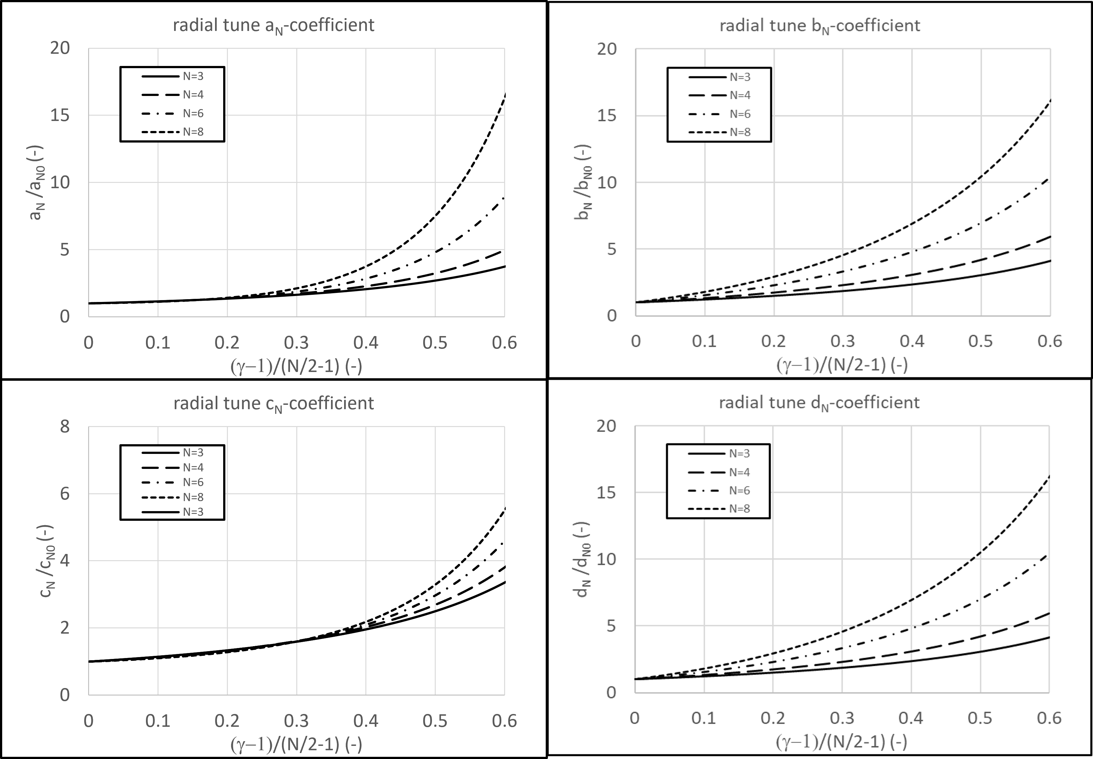
Figure 3: Energy dependence of the radial tune coefficients.

Note that the coefficients $\tilde{a}_{N},\tilde{b}_{N},\tilde{c}_{N},\tilde{d}_{N}$ are singular for $\gamma=N/2$ and for $\gamma=N$. The first singularity is due to the half-integer resonance which is treated separately in paragraph 5. The second singularity would happen far beyond the maximum energy that can be obtained in an isochronous cyclotron (see paragraph 6) and therefore is of no practical importance.

Figure 3 shows the energy dependence of the horizontal tune coefficients. The representation of the axes is the same as used in Figure 2. It is seen from Figure 3 that the coefficients may vary more than a factor 10 in the energy range considered. The energy dependency is higher for higher N-values. This makes sense because the absolue particle energy (for example at 60% scale value) increases almost linearly with $N$ and therefore also the radial derivatives of the isochronous field will increase substantially (see Figure 1).

In order to validate the derivations in this report, we compare results with those obtained for the C400 hadron therapy cyclotron. The design of this K=1600 machine was initiated around the year 2004[4] and finalized around the year 2010[5, 6]. Currently the machine is actually under construction in a collaboration between NHa and IBA. Figure 4 shows results of the Fourier analysis of the C400 magnetic field. The upper left shows the amplitudes of the first five structural Fourier components (normalized) a function of radius (as defined in appendix B.1) and the upper right figure shows the flutter (see Eq. (B20)) and its radial derivative. The flutter is roughly equal to $C_{4}^{2}/2$ in agreement with Eq. (B21). The lower left figure shows the spiral angles of each of the first five structural Fourier components. It is seen that they are closely the same for all five components. This property was used in the derivation of Eq. (47) and will also be used further on in the paper. The lower right figure shows different alternatives for the definition of the spiral angle. The first one uses the azimuth at which the magnetic field around a circle reaches its maximum. The second and third alternatives use the azimuth at which the azimuthal derivative of the magnetic field reaches its maximum (at sector entrance) or minimum (at sector exit) respectively. The fourth alternative uses the azimuth at which the basic harmonic component $C_{N}$ reaches its maximum. The first alternative is not a good choice, because it deviates too much at high radii. For the radial tune (and also for the $\nu_{r}=N/2$ stopband, to be derived later) the other three alternatives give closely the same results. However, for the vertical tune we find that the average of the second and third alternatives give the best match with the C400-tunes (see paragraph 4). This makes sense because it is at the sector entrance and exit where the strong vertical focusing takes place. We therefore use this definition in the paper.

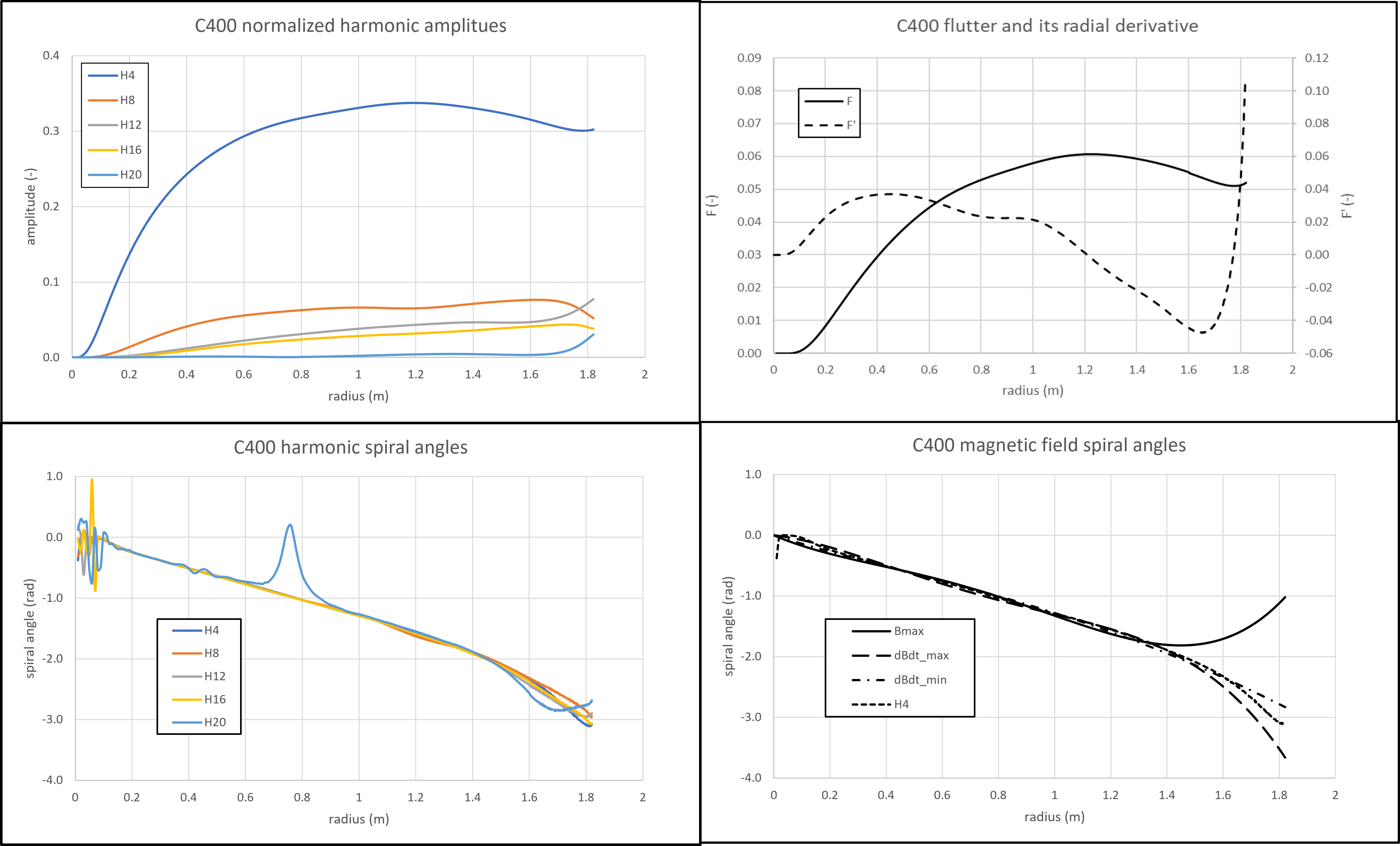
Figure 4: C400 harmonics and spiral angle comparisson

Figure 5 compares for the C400 our analytical radial tune (black curve, calculated with Eq. (47)) with the numerical tune obtained from a closed orbit code (blue curve). In the left figure the relativistic contribution to the tune (=$\gamma$) is also shown seperately (red curve). At extraction, this contribution accounts for almost 75% of the total. The right of Figure 5 shows the part of the radial tune that is due to the flutter only. Here there is a small difference between the analytical and the closed orbit results. This difference is likely due to the fact that in the derivation of Eq. (47)), we ignore the approach towards the half-integer resonance. As shown in Figure 17 the actual tune, when approaching the stopband, is higher than the “non-resonance” approximation of the tune. The dashed curve in the right of Figure 5 show the flutter contribution to the radial tune that is obtained if the energy-dependence of the tune-coefficients in Eq. (47) is ignored (by evaluating these coefficients at the value $\gamma=1$). This is equivalent to a derivation in which the cross-terms between the average field radial derivatives and the magnetic field Fourier terms are neglected. It is seen from the figure that such an approximation would have a big impact on the flutter contribution to the tune.

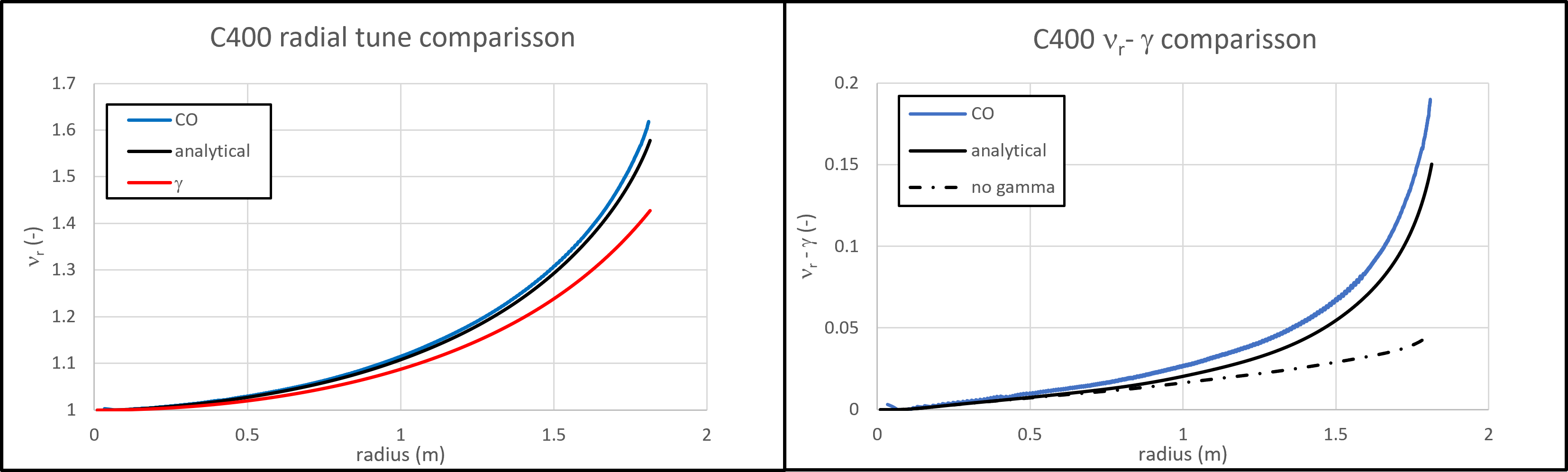
Figure 5: C400 radial tune comparisson

4 The linear vertical motion

The derivation of the vertical motion is very much similar to that of the linear radial motion as was done in paragraph 3.4. We start with the basic Hamiltonian for the vertical motion derived in pargraph A and given in Eq. (A30). We assume that the motion in the median plane follows the EO and therefore substitute in Eq. (A30) for $x,p_{x}$ the EO solution $x_{e},p_{e}$. In the coefficients of this Hamiltonian we have to keep constants up to $\mathscr{O}(f^{2})$ and oscillating terms up to $\mathscr{O}(f)$. We obtain:

$$K_{z}(\zeta,p_{z},\theta)=\tfrac{1}{2}\left(1+x_{e}+\tfrac{1}{2}\dot{x}_{e}^{2}\right)p_{z}^{2}+\tfrac{1}{2}\left(p_{e}\frac{\partial\mu}{\partial\theta}+(1-x_{e})\frac{\partial\mu}{\partial x}\right)\zeta^{2}\ .$$ (52)

Note that here, we have to evaluate $\frac{\partial\mu}{\partial\theta}$ and $\frac{\partial\mu}{\partial x}$ on the EO (so at $x=x_{e}$). We bring this Hamiltonian to its normal form by a canonical transformation $p_{z},\zeta\Rightarrow P_{z},Z$ using the method explained in paragraph G.4. This gives us for the new Hamiltonian $H_{z}(Z,P_{z})$:

$$\bar{K}_{z}(Z,P_{z})=\tfrac{1}{2}P_{z}^{2}+\tfrac{1}{2}Q_{z}(\theta)Z^{2}\ ,$$ (53)

where $Q(\theta)$ is obtained as:

$$Q_{z}(\theta)=\dot{x}_{e}\frac{\partial\mu}{\partial\theta}-(1+2x_{e}+x_{e}^{2}+\tfrac{1}{2}\dot{x}_{e}^{2})\frac{\partial\mu}{\partial x}+\tfrac{1}{2}\ddot{x}_{e}-\tfrac{1}{4}\dot{x}_{e}^{2}\ .$$ (54)

We calculate the partial derivatives $\frac{\partial\mu}{\partial\theta}$ and $\partial\mu/\partial x$ from the expression for the reduced field $\mu$ given in Eq. (B10) and insert them in Eq. (54). We obtain:

$$Q_{z}(\theta) =-\bar{\mu}^{\prime}-(2\bar{\mu}^{\prime}+\bar{\mu}^{\prime\prime})x_{e}-\tfrac{1}{2}(2\bar{\mu}^{\prime}+4\bar{\mu}^{\prime\prime}+\bar{\mu}^{\prime\prime\prime})x_{e}^{2}+\tfrac{1}{2}\ddot{x_{e}}-\tfrac{1}{4}(1+2\bar{\mu}^{\prime})\dot{x}_{e}^{2}$$

$$-\operatorname*{\textstyle\sum}_{n}\left[A^{\prime}_{n}+(2A^{\prime}_{n}+A^{\prime\prime}_{n})x_{e}-nB_{n}\dot{x}_{e}\right]\cos n\theta$$ (55)

$$-\operatorname*{\textstyle\sum}_{n}\left[B^{\prime}_{n}+(2B^{\prime}_{n}+B^{\prime\prime}_{n})x_{e}+nA_{n}\dot{x}_{e}\right]\sin n\theta\ .$$

We now work out this expresion in full detail. This is done with the following additional steps: i) use the expressions for $x_{e}$ and $\dot{x}_{e}$ as defined by Eqs. (3,4,5,6) and insert those in Eq. (55), ii) in the obtained result, split the $\mathscr{O}(f^{0})$ term $\bar{\mu}^{\prime}$ in its relativistic part and its flutter part as $\bar{\mu}^{\prime}=\bar{\mu}^{\prime}_{rel}+\bar{\mu}^{\prime}_{fl}$ and insert for $\bar{\mu}^{\prime}_{fl}$ the expression given in Eq. (27), iii) replace Fourier sine/cosine coefficients and their radial derivatives $A_{n},A^{\prime}_{n},A^{\prime\prime}_{n}$, $B_{n},B^{\prime}_{n},B^{\prime\prime}_{n}$ by Fourier amplitudes and their derivatives $C_{n},C^{\prime}_{n},C^{\prime\prime}_{n}$ and phase derivative $\varphi^{\prime}_{n}$ using Eqs. (B13-B15,B16), iv) of all the $\theta$-dependent terms of $\mathscr{O}(f^{2})$ keep only their average and v) substitute for the higher derivatives $\bar{\mu}^{\prime\prime},\bar{\mu}^{\prime\prime\prime}$ epressions envolving the field-index $\bar{\mu}^{\prime}$, using Eqs. (22,23).

We write the Hamiltonian in the same form as given in Eq. (C1):

$$\bar{K}_{z}(P_{z},Z,\theta)=\tfrac{1}{2}P_{z}^{2}+\tfrac{1}{2}(\nu_{z0}^{2}+f(\theta))Z^{2}\ .$$ (56)

We find for $\nu_{z0}^{2}$:

$$\nu_{z0}^{2}=-\bar{\mu}^{\prime}_{rel}+\tfrac{1}{8} \sum_{n}{{{[}}}\frac{n^{2}(4n^{2}-5)+12\bar{\mu}^{\prime}(n^{2}-(1+\bar{\mu}^{\prime})(2+\bar{\mu}^{\prime}))}{(n^{2}-1-\bar{\mu}^{\prime})^{2}}$$

$$-4\bar{\mu}^{\prime}\frac{(n^{2}-1)(3n^{2}-7-\bar{\mu}^{\prime}(11+\bar{\mu}^{\prime}))-3\bar{\mu}^{\prime 2}}{(n^{2}-1-\bar{\mu}^{\prime})^{3}}{{{]}}}C_{n}^{2}$$ (57)

$$+ \sum_{n}\frac{n^{2}-1+\bar{\mu}^{\prime}(3+4\bar{\mu}^{\prime})}{2(n^{2}-1-\bar{\mu}^{\prime})^{2}}C_{n}C^{\prime}_{n}+\sum_{n}\frac{C^{\prime 2}_{n}+n^{2}C_{n}^{2}\varphi^{\prime 2}_{n}}{2(n^{2}-1-\bar{\mu}^{\prime})}\ .$$

And $f(\theta)$ is defined by:

$$f(\theta) =\sum_{n}a_{n}\cos n\theta+b_{n}\sin n\theta\ ,$$

$$a_{n} =-\tfrac{1}{2}\frac{n^{2}+6\bar{\mu}^{\prime}(1+\bar{\mu}^{\prime})}{n^{2}-1-\bar{\mu}^{\prime}}A_{n}-A^{\prime}_{n}\ ,$$ (58)

$$b_{n} =-\tfrac{1}{2}\frac{n^{2}+6\bar{\mu}^{\prime}(1+\bar{\mu}^{\prime})}{n^{2}-1-\bar{\mu}^{\prime}}B_{n}-B^{\prime}_{n}\ .$$

In paragraph C the general solution of a Hamiltonian with the structure of Eq. (56) has been derived by a canonical transformation that transforms the oscillating function $f(\theta)$ to the next higher order $\mathscr{O}(f^{2})$. The final Hamiltonian has the form:

$$\bar{K}_{z}(P_{z},Z,\theta)=\tfrac{1}{2}P_{z}^{2}+\tfrac{1}{2}\nu_{z}^{2}Z^{2}\ ,$$ (59)

where:

$$\nu_{z}^{2}=\nu_{z0}^{2}+\tfrac{1}{2}\sum_{n}\frac{a_{n}^{2}+b_{n}^{2}}{n^{2}-4\nu_{z0}^{2}}\ .$$ (60)

The expression for the tune becomes:

$$\nu_{z}^{2}=-\bar{\mu}^{\prime}_{rel}+ \sum_{n}{{{[}}}\frac{\left(n^{2}+6\bar{\mu}^{\prime}(1+\bar{\mu}^{\prime})\right)^{2}}{n^{2}+4\bar{\mu}^{\prime}}+n^{2}(4n^{2}-5)+12\bar{\mu}^{\prime}(n^{2}-2-3\bar{\mu}^{\prime}-\bar{\mu}^{\prime 2})$$

$$-4\bar{\mu}^{\prime}\frac{(n^{2}-1)(3n^{2}-7-\bar{\mu}^{\prime}(11+\bar{\mu}^{\prime}))-3\bar{\mu}^{\prime 3}}{n^{2}-1-\bar{\mu}^{\prime}}{{{]}}}\frac{C_{n}^{2}}{8(n^{2}-1-\bar{\mu}^{\prime})^{2}}$$

$$+ \sum_{n}\frac{(2n^{2}-1+3\bar{\mu}^{\prime})(C_{n}^{\prime 2}+n^{2}C_{n}^{2}\varphi^{\prime 2})}{2(n^{2}+4\bar{\mu}^{\prime})(n^{2}-1-\bar{\mu}^{\prime})}$$

$$+ \sum_{n}{{{[}}}\frac{n^{2}++5\bar{\mu}^{\prime}+3\bar{\mu}^{\prime 2}}{n^{2}+4\bar{\mu}^{\prime}}+\frac{2\bar{\mu}^{\prime}(1+\bar{\mu}^{\prime})}{n^{2}-1-\bar{\mu}^{\prime}}{{{]}}}\frac{C_{n}C^{\prime}_{n}}{n^{2}-1-\bar{\mu}^{\prime}}$$ (61)

This is a very complex and rather impractical formula. We simplify it by the method explained in paragraph B.4 and substitute for the Fourier coefficient $C_{n}$ their expressions in terms of the flutter $F$ as defined in Eqs. (LABEL:CtoF). We write the result as follows:

$$\boxed{\nu_{z}^{2}=-\bar{\mu}^{\prime}_{rel}+\frac{8N^{2}F}{\pi^{2}}\left[\hat{a}_{N}+\hat{b}_{N}\varphi^{\prime 2}+\hat{c}_{N}\frac{F^{\prime}}{F}+\hat{d}_{N}\left(\frac{F^{\prime}}{F}\right)^{2}\right]\ .}$$ (62)

Here the functions $\hat{a}_{N},\hat{b}_{N},\hat{c}_{N},\hat{d}_{N}$ depend only on the symmetry number $N$ and on the relativistic parameter $\gamma$ via the relation $\bar{\mu}^{\prime}=\bar{\mu}^{\prime}_{rel}=\gamma^{2}-1$.

The expressions for these parameters are given by:

$$\hat{a}_{N} =\sum_{k=0}^{\infty}\frac{1}{4n^{2}(n^{2}-1-\bar{\mu}^{\prime})^{2}}{{[}}-4\bar{\mu}^{\prime}\frac{(n^{2}-1)(3n^{2}-7-\bar{\mu}^{\prime}(11+\bar{\mu}^{\prime}))-3\bar{\mu}^{\prime 3}}{n^{2}-1-\bar{\mu}^{\prime}}$$

$$\ \hskip 14.22636pt+\frac{\left(n^{2}+6\bar{\mu}^{\prime}(1+\bar{\mu}^{\prime})\right)^{2}}{n^{2}+4\bar{\mu}^{\prime}}+n^{2}(4n^{2}-5)+12\bar{\mu}^{\prime}(n^{2}-(1+\bar{\mu}^{\prime})(2+\bar{\mu}^{\prime})){{]}}\ ,$$

$$\hat{b}_{N} =\sum_{k=0}^{\infty}\frac{2n^{2}-1+3\bar{\mu}^{\prime}}{(n^{2}+4\bar{\mu}^{\prime})(n^{2}-1-\bar{\mu}^{\prime})}=\sum_{k=0}^{\infty}\frac{1}{n^{2}+4\bar{\mu}^{\prime}}+\frac{1}{n^{2}-1-\bar{\mu}^{\prime}}\ ,$$ (63)

$$\hat{c}_{N} =\sum_{k=0}^{\infty}\frac{1}{n^{2}(n^{2}-1-\bar{\mu}^{\prime})}{{[}}\frac{n^{2}+\bar{\mu}^{\prime}(5+3\bar{\mu}^{\prime})}{n^{2}+4\bar{\mu}^{\prime}}+\frac{2\bar{\mu}^{\prime}(1+\bar{\mu}^{\prime})}{n^{2}-1-\bar{\mu}^{\prime}}{{]}}\ ,$$

$$\hat{d}_{N} =\sum_{k=0}^{\infty}\frac{2n^{2}-1+3\bar{\mu}^{\prime}}{4n^{2}(n^{2}+4\bar{\mu}^{\prime})(n^{2}-1-\bar{\mu}^{\prime})}\ .$$

In these equations we have to replace $n$ by $n=(2k+1)N$.

The summations in Eqs. (63) can be done analytically and the coefficients $\hat{a}_{N},\hat{b}_{N},\hat{c}_{N},\hat{d}_{N}$ can be expressed in elementary mathematical functions. Appendix E shows how this is done. We find the following result:

$$\hat{a}_{N}(\gamma) =\hat{q}_{1}\tan(\frac{\pi\gamma}{2N})+\hat{q}_{2}\tanh(\frac{\pi\sqrt{\gamma^{2}-1}}{N})+\hat{q}_{3}(1+\tan^{2}(\frac{\pi\gamma}{2N}))+\hat{q}_{4}$$

$$\ \hskip 69.70915pt+\hat{q}_{5}\tan(\frac{\pi\gamma}{2N})(1+\tan^{2}(\frac{\pi\gamma}{2N}))\ ,$$

$$\hat{b}_{N}(\gamma) =\frac{\pi}{8N\gamma}{{{(}}}2\tan(\frac{\pi\gamma}{2N})+\frac{\gamma}{\sqrt{\gamma^{2}-1}}\tanh(\frac{\pi\sqrt{\gamma^{2}-1}}{N}){{{)}}}\ ,$$

$$\hat{c}_{N}(\gamma) =\frac{\pi^{2}(9\gamma^{2}-14)}{32N^{2}\gamma^{2}}-\frac{\pi(12\gamma^{4}-27\gamma^{2}+14)}{4N\gamma^{3}(5\gamma^{2}-4)}\tan(\frac{\pi\gamma}{2N})$$

$$+\frac{\pi^{2}(\gamma^{2}-1)}{8N^{2}\gamma^{2}}\tan^{2}(\frac{\pi\gamma}{2N})+\frac{\pi(3\gamma^{2}-2)}{32N(5\gamma^{2}-4)\sqrt{\gamma^{2}-1}}\tanh(\frac{\pi\sqrt{\gamma^{2}-1}}{N})\ ,$$

$$\hat{d}_{N}(\gamma) =\frac{\pi}{128N^{2}\gamma^{3}}{{{(}}}\frac{\pi\gamma(4-3\gamma^{2})}{\gamma^{2}-1}+8N\tan(\frac{\pi\gamma}{2N})-\frac{N\gamma^{3}}{(\gamma^{2}-1)^{3/2}}\tanh(\frac{\pi\sqrt{\gamma^{2}-1}}{N}){{{)}}}\ ,$$

Here the coefficients $\hat{q}_{i}$ are defined as:

$$\hat{q}_{1}(\gamma) =\frac{\pi}{32N\gamma^{3}}{{[}}84\gamma^{4}-176\gamma^{2}+101-\frac{(6\gamma^{2}-5)(102\gamma^{4}-177\gamma^{2}+76)\gamma^{2}}{(5\gamma^{2}-4)^{2}}{{]}}\ ,$$

$$\hat{q}_{2}(\gamma) =\frac{\pi}{256N}\frac{(9\gamma^{4}-12\gamma^{2}+32)\sqrt{\gamma^{2}-1}}{(5\gamma^{2}-4)^{2}}\ ,$$

$$\hat{q}_{3}(\gamma) =\frac{\pi^{2}}{64N^{2}}{{[}}\frac{(6\gamma^{2}-5)^{2}}{5\gamma^{2}-4}-\frac{36\gamma^{4}-80\gamma^{2}+45}{\gamma^{2}}{{]}}\ ,$$ (64)

$$\hat{q}_{4}(\gamma) =-\frac{\pi^{2}}{32N^{2}\gamma^{2}}(\gamma^{2}-1)(15\gamma^{2}-28)\ ,$$

$$\hat{q}_{5}(\gamma) =\frac{\pi^{3}}{16N^{3}\gamma}(\gamma^{2}-1)^{2}\ .\$$

Note that the expressions for $\hat{b}_{N},\hat{c}_{N},\hat{d}_{N}$ are singular for $\gamma=1$ and the limits for $\gamma\downarrow 1$ need to be taken. These limits are as follows:

$$\hat{a}_{N}(1) =\frac{\pi}{4N}\tan(\frac{\pi}{2N})\ ,$$

$$\hat{b}_{N}(1) =\frac{\pi}{8N}{{(}}\frac{\pi}{N}+2\tan(\frac{\pi}{2N}){{)}}\ ,$$

$$\hat{c}_{N}(1) =\frac{\pi}{4N}{{(}}-\frac{\pi}{2N}+\tan(\frac{\pi}{2N}){{)}}\ ,$$

$$\hat{d}_{N}(1) =\frac{\pi}{128N^{2}}{{(}}-4\pi+\frac{\pi^{3}}{3N^{2}}+8N\tan(\frac{\pi}{2N}){{)}}\ .$$

Figure 6 shows the energy dependence of the vertical tune coefficients. The representation of the axes is the same as used in Figure 2. It is seen that the coefficient $\hat{c}_{N}$ may vary more than a factor 10 in the energy range considered. However, for higher energies, the most important contribution to the vertical tune by far comes from the spiraling of the sectors, i.e. from the coefficient $\hat{b}_{N}$. This coefficient depends only weakly on energy. As can be seen from Eqs. (63) the equation for $\hat{b}_{N}$ contains two terms with opposite energy dependence and therefore there is some cancellation of this dependence. For that reason the cross terms between $\bar{\mu}$-derivatives and flutter terms are less importance in the derivation of the vertical tune.

Figure 7 compares for the C400 our analytical vertical tune (black curve, calculated with Eq. (62)) with the numerical tune obtained from a closed orbit code (CO=blue curve). The vertical tune depends critically on the definition of the spiral angle. The main reason for this is that the tune (squared) is obtained as the difference between two larger numbers (the field index $\bar{\mu}^{\prime}$ as a negative contribution and the flutter as a positive contribution), which to a substantial degree cancel eached other.

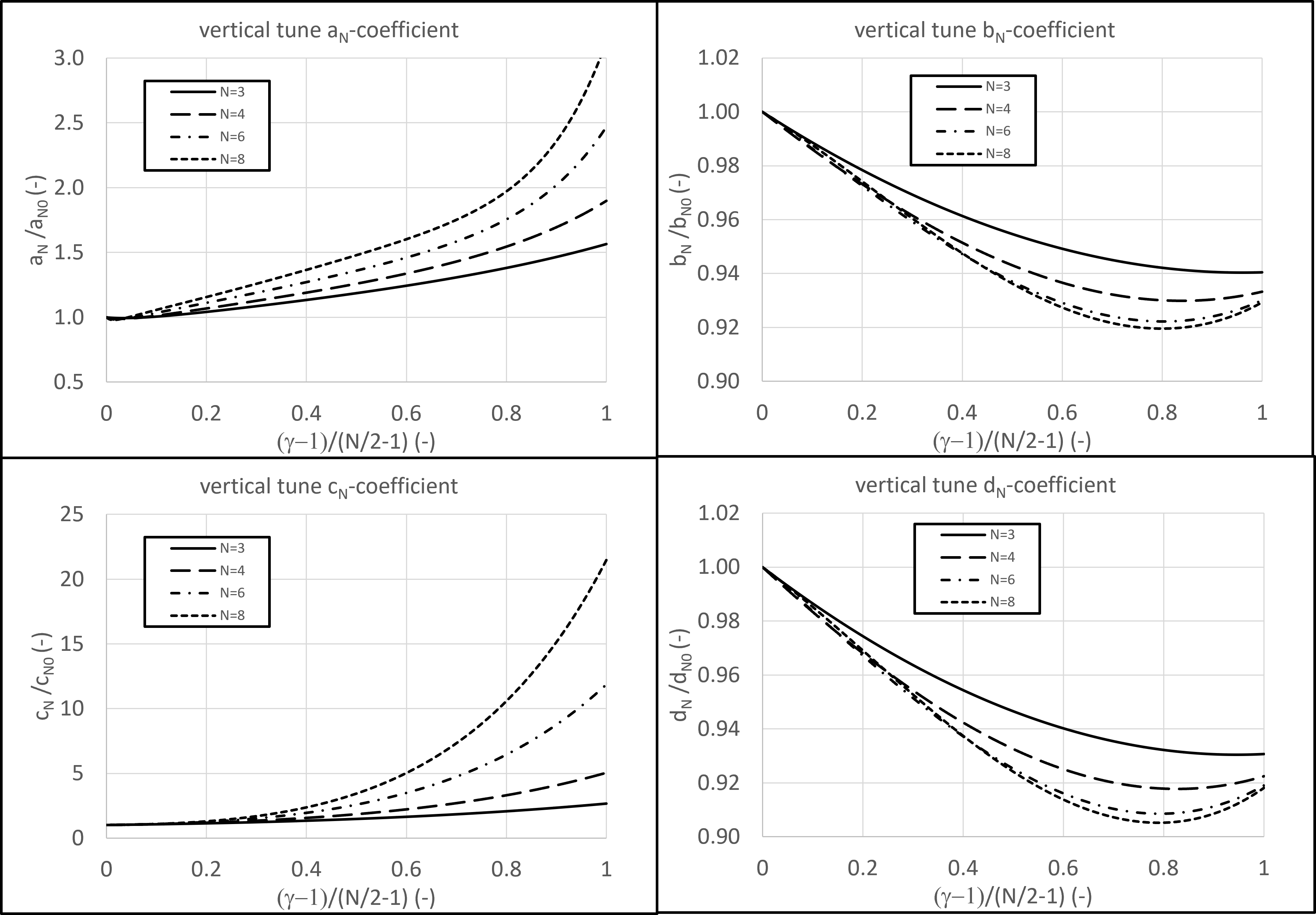
Figure 6: Energy dependence of the vertical tune coefficients.

Different alternatives for the definition of the spiral angle have been introduced in paragraph 3.4 and the corresponding tunes are shown in the figure on the left. The red curve (Bmax) uses the spiral angle obtained from the azimuth where the magnetic field around a circle is maximum. This model fits well up to a radius of about 1.2 m ($\approx$125 MeV/u), but beyond that immediately collapses. The orange curve (H4), based on the azimuth of the basic harmonic $C_{4}$, gives some improvement but is still not satisfactory. The green curve (edges), based on the average of the sector-in and sector-out azimuths, shows a further improvement but it still deviates substantially from the numerical curve. The black curve shows our final result where the spiral angle (corresponding to the previous case) has been corrected for the fact that the equilibrium orbit is not a circle and therefore enters and exits from the sector with a non-zero radial momentum. This correction is explained in paragraph 3.2 and Eq. (9) was used to calculate it.

The dashed curve (corr) in Figure 7 shows the same case but here the flutter contribution to the vertical tune is obtained by ignoring the energy-dependence of the tune-coefficients in Eq. (62) (by evaluating those at the value $\gamma=1$). This is equivalent to using a derivation in which the cross-terms between the average field radial derivatives and the magnetic field Fourier terms are neglected. It is seen from the figure that such an approximation does not have such a big impact on the resulting tune. The dotted curve in the right frame of Figure 7 shows a case where the contribution of the flutter radial derivative to the vertical tune is ignored. It is seen that this contribution is small at high energies where the effect of the spiral angles dominates. For smaller machines with little or no spiralling the $F^{\prime}$-contribution may be more significant, especially in the extraction region where the flutter usually starts to drop.

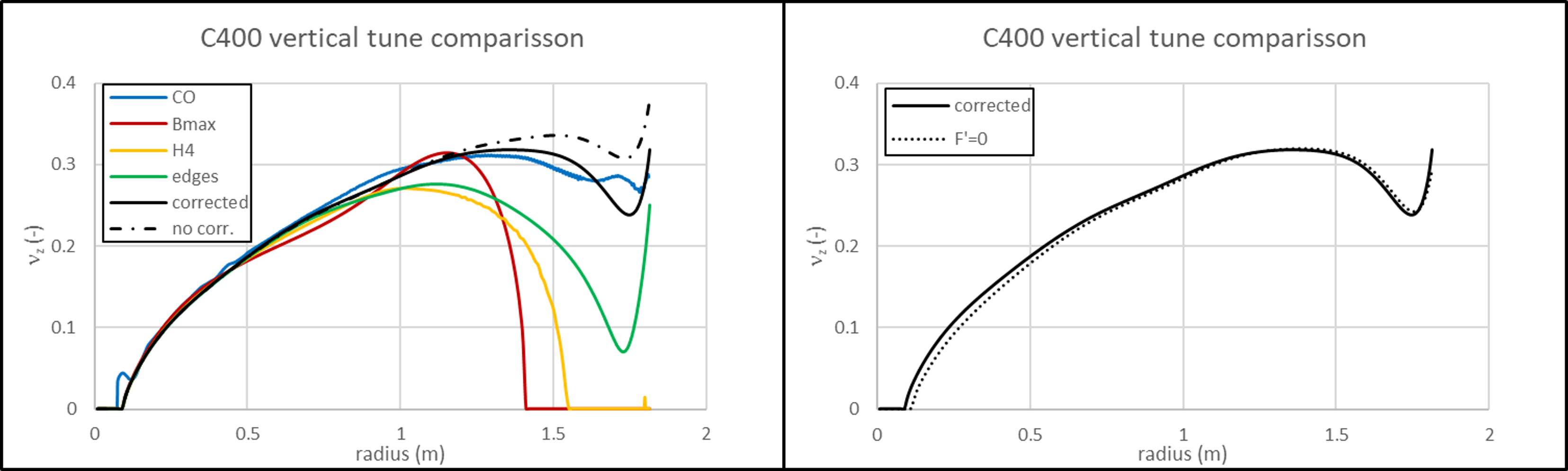
Figure 7: C400 vertical tune comparisson

5 The stopband of the half-integer resonance

In paragraph D a general treatment is given of the half-integer resonance for a Hamiltonian of the form given in Eq. (C1). In this paragraph those results are used to find the $\nu_{r}=N/2$ stopband of the isochronous cyclotron. The general expression for the stopband is given in Eq. (D40). In this equation we must insert expressions for $\nu_{0}$ and $c_{n}$ as applicable for the isochronous cyclotron. These have been derived in paragraph 3.4. For $\nu_{0}$ we must insert the expression for $\nu_{x0}$ as given in Eq. (42). With this we can write for the relativistic gamma parameters of the stopband:

$$\gamma_{1,2}=\frac{N}{2}\mp\frac{c_{N}}{2N}-\Delta_{1}-\Delta_{2}\ ,$$ (65)

where $\gamma$ is the relativistic gamma and where the expression for $\Delta_{1}$ is given in Eq. (42) and the expression for $\Delta_{2}$ in Eq. (D41) . The expression for $c_{n}$ we obtain from Eq. (43):

$$c_{n}^{2}=a_{n}^{2}+b_{n}^{2}=\left[\left(\tfrac{3}{2}\frac{n^{2}+2\bar{\mu}^{\prime}(1+\bar{\mu}^{\prime})}{n^{2}-1-\bar{\mu}^{\prime}}+\frac{C_{n}^{\prime}}{C_{n}}\right)^{2}+n^{2}\varphi_{n}^{\prime 2}\right]C_{n}^{2}\ .$$ (66)

The parameters $c_{n},\Delta_{1},\Delta_{2}$ depend on the energy $\gamma$ through their dependence on $\bar{\mu}^{\prime}$. Therefore Eq. (65) represents an implicit expression for the stopband limits $\gamma_{1,2}$. We can solve for $\gamma_{1,2}$ by using successive substitution in three steps. The goal is to find the stopband limits up to order $\mathscr{O}(f^{2})$. The first step gives the stopband limits up to order $\mathscr{O}(f^{0})$. Since $c_{n}$ is $\mathscr{O}(f^{1})$ and $\Delta_{1},\Delta_{2}$ are $\mathscr{O}(f^{2})$, we get:

$$\gamma^{(0)}_{1,2} =\frac{N}{2}\ ,$$ (67)

$$\gamma^{(1)}_{1,2} =\frac{N}{2}\mp\frac{c_{N}(\gamma^{(0)})}{2N}\ .$$ (68)

In the second equation the term $c_{N}$ must be evaluated at $\gamma=N/2$. This means for $\bar{\mu}^{\prime}=\gamma^{2}-1=\tfrac{N^{2}}{4}-1$. Using this in Eq. (66) one finds after the second step of successive substitution:

$$\gamma^{(1)}_{1,2}=\frac{N}{2}\mp\frac{C_{N}}{2N}\sqrt{{{(}}1+\frac{N^{2}}{4}+\frac{C_{N}^{\prime}}{C_{N}}{{)}}^{2}+N^{2}\varphi^{\prime 2}_{N}}\ .$$ (69)

The third step of successive substitution can now be written as:

$$\gamma^{(2)}_{1,2}=\frac{N}{2}\mp\frac{c_{N}(\gamma^{(1)})}{2N}-\Delta_{1}(\gamma^{(0)})-\Delta_{2}(\gamma^{(0)})\ .$$ (70)

The second term for $c_{N}$ in this equation must now be evaluated at $\gamma^{(1)}$ which is given in Eq. (69). To do this we write $c_{N}$ as a function of energy $\gamma$ as follows:

$$c_{N}(\gamma)=C_{N}\sqrt{{{(}}\tfrac{3}{2}\frac{N^{2}+2\gamma^{2}(\gamma^{2}-1)}{N^{2}-\gamma^{2}}+\frac{C_{N}^{\prime}}{C_{N}}{{)}}^{2}+N^{2}\varphi_{N}^{\prime 2}}\ ,$$ (71)

and do a Taylor expansion up to first degree:

$$c^{(2)}_{N}=c_{N}(\gamma^{(1)})=c_{N}(\tfrac{N}{2}+\delta)=c_{N}(\tfrac{N}{2})+\delta\frac{dc_{N}}{d\gamma}|_{\gamma=N/2}\ ,$$ (72)

where $\delta=\gamma^{(1)}-\tfrac{N}{2}$ is obtained from Eq. (69). We calculate $c^{(2)}_{N}$ up to $\mathscr{O}(f^{2})$ and get:

$$\frac{c_{N}^{(2)}}{2N} =\frac{C_{N}}{2N}\sqrt{{{(}}1+\frac{N^{2}}{4}+\frac{C_{N}^{\prime}}{C_{N}}{{)}}^{2}+N^{2}\varphi^{\prime 2}_{N}}-\Delta_{3}\ ,$$ (73)

$$\Delta_{3} =\frac{(7N^{2}-8)}{12N^{3}}{{(}}1+\frac{N^{2}}{4}+\frac{C_{N}^{\prime}}{C_{N}}{{)}}C_{N}^{2}\ .$$ (74)

In this way the stopband limits can be writen as:

$$\gamma_{1,2} =\frac{N}{2}\mp\frac{C_{N}}{2N}\sqrt{{{(}}1+\frac{N^{2}}{4}+\frac{C_{N}^{\prime}}{C_{N}}{{)}}^{2}+N^{2}\varphi^{\prime 2}_{N}}-\Delta\ ,$$ (75)

$$\Delta =\Delta_{1}+\Delta_{2}+\Delta_{3}\ .$$ (76)

Here the terms $\Delta_{1}$ and $\Delta_{2}$ are both of $\mathscr{O}(f^{2})$ and therefore they can be evaluated at the energy $\gamma=\gamma^{(0)}=N/2$. We find for $\Delta_{1}$ and $\Delta_{2}$:

$$\Delta_{1} =\frac{1}{2N}\sum_{n=N}{{{(}}}\frac{12n^{2}+\tfrac{1}{2}N^{2}(N^{2}-4)(N^{2}-6)}{(4n^{2}-N^{2})^{2}}-4\frac{n^{2}\varphi_{n}^{\prime 2}}{4n^{2}-N^{2}}$$

$$\hskip 56.9055pt-\frac{(N^{2}-4)^{2}(16+(N^{2}-4)(\tfrac{N^{2}}{4}+10))}{(4n^{2}-N^{2})^{3}}{{{)}}}C_{n}^{2}$$ (77)

$$-\frac{1}{2N}\sum_{n=N}{{{(}}}\frac{4(n^{2}-1)+(N^{2}-1)(N^{2}-4)}{n^{2}(4n^{2}-N^{2})}C_{n}C_{n}^{\prime}+\frac{4C_{n}^{\prime 2}}{n^{2}(4n^{2}-N^{2})}{{{)}}}\ ,$$ (78)

$$\Delta_{2} =\frac{3C_{N}^{2}}{8N^{3}}{{{(}}}(1+\frac{N^{2}}{4}+\frac{C_{N}^{\prime}}{C_{N}})^{2}+N^{2}\varphi_{N}^{\prime 2}{{{)}}}+\frac{3}{4N}\sum_{n>N}\frac{(8n^{2}+N^{2}(N^{2}-4))}{(4n^{2}-N^{2})(n^{2}-N^{2})}C_{n}C_{n}^{\prime}$$

$$+\frac{1}{2N}\sum_{n>N}{{{(}}}\frac{9}{16}\frac{{{(}}8n^{2}+N^{2}(N^{2}-4){{)}}^{2}}{(4n^{2}-N^{2})^{2}(n^{2}-N^{2})}+\frac{n^{2}\varphi_{n}^{\prime 2}}{n^{2}-N^{2}}{{{)}}}C_{n}^{2}+\frac{1}{2N}\sum_{n>N}\frac{C_{n}^{\prime 2}}{n^{2}-N^{2}}\ ,$$ (79)

As before, we eliminate the Fourier coefficients $C_{n}$ in favor of the flutter $F$ using the method explained in paragraph B.4 and assume that the spiral angles of all harmonics are equal ($\varphi^{\prime}_{n}=\varphi^{\prime}_{N}=\varphi^{\prime}$). We write the stopband limits as follows:

$$\gamma_{1,2}=\frac{N}{2} \mp\frac{2\sqrt{F}}{\pi N}\sqrt{{{(}}1+\frac{N^{2}}{4}+\frac{F^{\prime}}{2F}{{)}}^{2}+N^{2}\varphi^{\prime 2}_{N}}$$

$$-\frac{F}{\pi^{2}N^{3}}\left(\bar{a}_{N}-\bar{b}_{N}\varphi^{\prime 2}-\bar{c}_{N}\frac{F^{\prime}}{F}+\bar{d}_{N}(\frac{F^{\prime}}{F})^{2}\right)\ .$$ (80)

Here $\bar{a}_{N},\bar{b}_{N},\bar{c}_{N},\bar{d}_{N}$ are defined as:

$$\bar{a}_{N}=6(1+\frac{N^{2}}{4})^{2}+\frac{1}{3}(N^{2}+4)(7N^{2}-8)+\frac{9}{32}\operatorname*{\textstyle\sum}_{k=1}\frac{(8m^{2}+(N^{2}-4))^{2}}{m^{2}(m^{2}-\tfrac{1}{4})^{2}(m^{2}-1)}$$

$$+\frac{1}{2}\operatorname*{\textstyle\sum}_{k=0}{{{(}}}\frac{12m^{2}+\tfrac{1}{2}(N^{2}-4)(N^{2}-6)}{m^{2}(m^{2}-\tfrac{1}{4})^{2}}-\frac{(N^{2}-4)^{2}(16+(N^{2}-4)(\tfrac{N^{2}}{4}+10))}{4N^{4}m^{2}(m^{2}-\tfrac{1}{4})^{3}}{{{)}}}\ ,$$

$$\bar{b}_{N}=8N^{2}{{{(}}}-\frac{3}{4}+\operatorname*{\textstyle\sum}_{k=0}\frac{1}{m^{2}-\tfrac{1}{4}}-\operatorname*{\textstyle\sum}_{k=1}\frac{1}{m^{2}-1}{{{)}}}\ ,$$ (81)

$$\bar{c}_{N}=\frac{4+37N^{2}}{6}-\frac{1}{4}\sum_{k=0}\frac{4m^{2}+N^{2}-5}{m^{2}(m^{2}-\tfrac{1}{4})^{2}}+\frac{3}{2}\sum_{k=1}\frac{8m^{2}+N^{2}-4}{m^{2}(m^{2}-\tfrac{1}{4})(m^{2}-1)}\ ,$$

$$\bar{d}_{N}=-\frac{3}{2}+\operatorname*{\textstyle\sum}_{k=0}\frac{2}{m^{2}(m^{2}-\tfrac{1}{4})}-\operatorname*{\textstyle\sum}_{k=1}\frac{2}{m^{2}(m^{2}-1)}\ ,$$

where we must substitute $m$ by $m=2k+1$, with $k=(0,)1,2,\dots$. The series can again be summed analytically (see appendix E) giving:

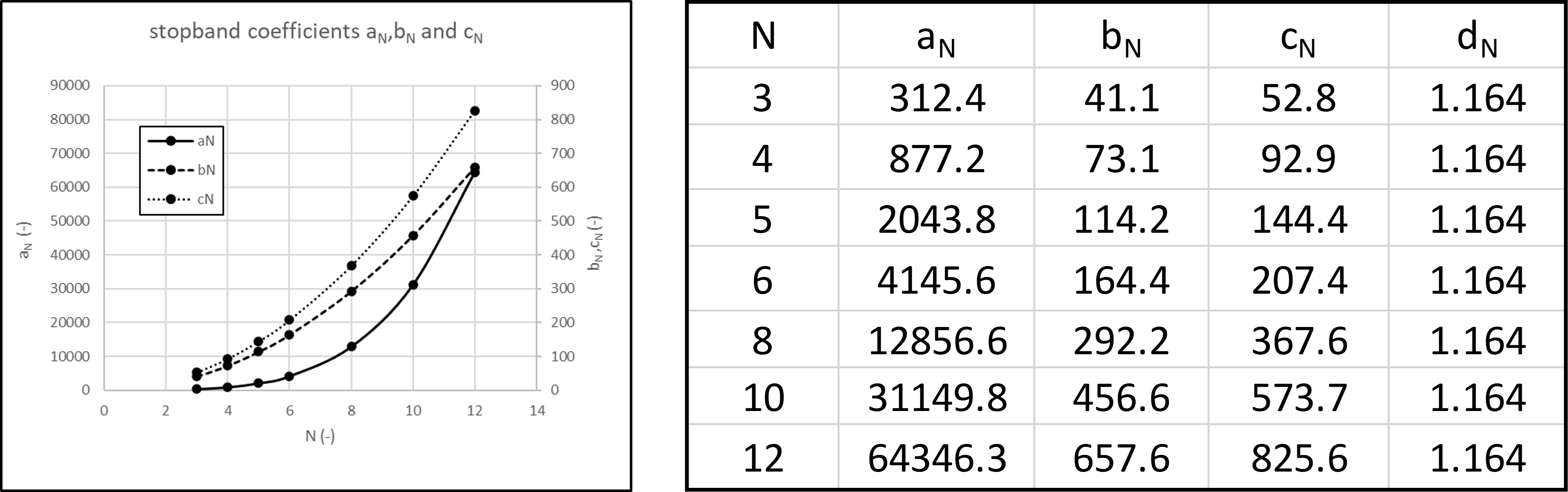
Figure 8: Stopband coefficients.

$$\bar{a}_{N} =\frac{-16+52N^{2}+14N^{4}}{3}+\pi(-40+4N^{2}+\frac{N^{4}}{2})+5\pi^{2}(3-\frac{N^{2}}{2}-\frac{N^{4}}{16})$$

$$-\frac{\pi}{32N^{4}}(\pi^{2}-22\pi+60)(N^{2}-4)^{2}(N^{4}+36N^{2}-96)\ ,$$ (82)

$$\bar{b}_{N} =8N^{2}(\frac{\pi}{2}-1)\ ,$$

$$\bar{c}_{N} =\frac{16}{3}-6\pi+\frac{3\pi^{2}}{2}+(\frac{34}{3}-\pi-\frac{\pi^{2}}{4})N^{2}\ ,$$

$$\bar{d}_{N} =-4+4\pi-\frac{3\pi^{2}}{4}\ .$$ (83)

Figure 8 graphically shows the dependence of the coefficients $\bar{a}_{N},\bar{b}_{N},\bar{c}_{N},\bar{d}_{N}$ on the cyclotron symmetry number $N$ and gives their values for a range of $N$-numbers. Figure 9 shows the stopband calculated from Eq. (80) for cyclotron symmetry numbers $N$ of 3,4,6,8,10,12 and for the case where the radial derivatives of the flutter are zero ($F^{\prime}=0$). The horizontal axis in the figures gives the flutter $F$ in logarithmic scale. The left axis gives the lower limit ($\gamma_{1}$, solid lines) and the right axis the width ($\gamma_{2}-\gamma_{1}$, dashed lines) of the stopband respectively. Both axes use the same scale as introduced in Figure 3. Results are shown for spiral angles of 45°,60°,70°,75° and 80°. It is seen that the lower stopband limit (i.e. the stable region) decreases monotonically with increasing flutter and increasing spiral angle. The normalized limit $(\gamma-1)/(\tfrac{N}{2}-1)$ increases monotonically with increasing N-number.

The stable region for a given spiral angle is the area under the curve between $\gamma=1$ and $\gamma=\gamma_{1}$. We note that for low symmetry numbers, there appears a second branch of $\gamma_{1}$ for high values of $F$ and large spiral angles. This artefact shows that the $\mathscr{O}(f^{2})$ approximation is not sufficient for very large flutter and/or spiral angle. Note that the maximum value of $F=1$ used in Figure 9 is really large, especially if combined with a large spiral angle. We further note that the convergence of the development is determined not so much by the magnitude of $f$ but by the magnitude of $f/N^{2}$. The reason for this is that the scalloping of the equilibrium orbit is proportional to $f/N^{2}$. and therefore, the EO becomes more and more circular for higher N-values. The branch therefore does not appear for the larger $N$ values. Note further that the apperance of this artificial branch does not compromise in any way the validity of the results because it occurs at $F$ values that are about an order of magnitude larger than the maximum $F$-value of the corresponding stability zone. It is this value that we are interested in. The artificial branch can therefore be ignored completely. It is seen from Figure 9 that the width of the stopband quickly rises to large values, for reasonable values of flutter and spiral angles. This shows that the half-integer resonance is extremely strong and impossible to cross by fast acceleration. It is a hard limit for the maximum energy of an isochronous cyclotron.

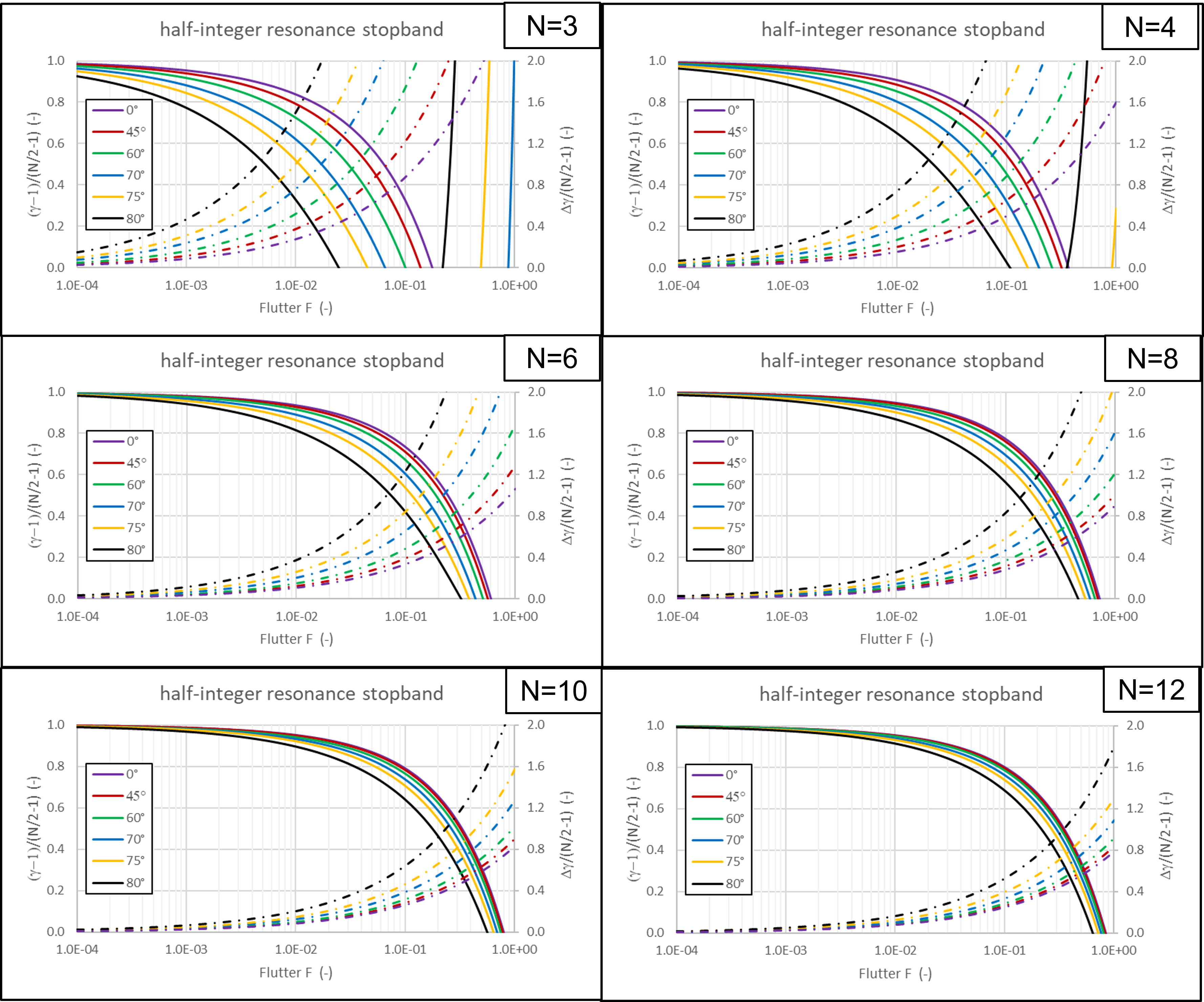
Figure 9: Stopband limit and width

5.1 Impact of different types of approximations

In the previous paragraph we derived the stopband of the half-integer resonance in a very accurate manner namely i) up to $\mathscr{O}(f^{2})$ in the magnetic field variation and ii) including terms that correlate derivatives of the average field $\bar{\mu}^{\prime},\bar{\mu}^{\prime\prime},\bar{\mu}^{\prime\prime\prime}$ with the azimuhal magnetic field variation $f$. However, both refinements make that the derivation is complex and elaborate. In this paragraph we investigate how these refinements impact the final result. For this purpose we re-calcuate the stopband limits by ignoring the cross-correlations. We label this as a non-relativistic approximation, because at low energies the average field derivatives and therefore also the correlating terms, are small. For simplicity we assume here that the radial derivative of the flutter equals zero ($F^{\prime}=0$). The approximation is found in a similar way as used in the previous paragraph but now we insert $\bar{\mu}^{\prime}=0$ in the expressions for $\Delta_{1}$ (in Eq. (42)) and $c_{n}$ (in Eq. (66)). The expression for $\Delta_{2}$ also needs to be re-calculated as it depends on $c_{n}$ (see Eq. (D41)). Further we have $\Delta_{3}=0$ for this case. We find for the stopband:

$$\gamma_{1,2} =\frac{N}{2}\mp\frac{C_{N}}{2}\sqrt{\frac{9N^{2}}{4(N^{2}-1)^{2}}+\varphi^{\prime 2}_{N}}-\Delta_{1}-\Delta_{2}\ ,$$ (84)

$$\Delta_{1} =\frac{2}{N}\sum_{n}\left(\frac{3n^{2}C_{n}^{2}}{16(n^{2}-1)^{2}}-\frac{n^{2}C_{n}^{2}\varphi^{\prime 2}_{n}}{4(n^{2}-1)}\right)\,$$ (85)

$$\Delta_{2} =\frac{3C_{N}^{2}}{8N}\left(\frac{9N^{2}}{4(N^{2}-1)^{2}}+\varphi^{\prime 2}_{N}\right)$$

$$+\frac{1}{2N}\sum_{n>N}n^{2}C_{n}^{2}\left(\frac{9n^{2}}{4(n^{2}-1)^{2}(n^{2}-N^{2})}+\frac{\varphi^{\prime 2}_{n}}{n^{2}-N^{2}}\right)\ .$$ (86)

We again eliminate the Fourier coefficients $C_{n}$ in favor of the flutter $F$ and write the stopband limits in the non-relativistic approximation as follows:

$$\gamma_{1,2}=\frac{N}{2}\mp\frac{2\sqrt{F}}{\pi}\sqrt{\frac{9N^{2}}{4(N^{2}-1)^{2}}+\varphi^{\prime 2}_{N}}-\frac{F}{\pi^{2}N^{3}}(a_{N}-b_{N}\varphi^{\prime 2})\ ,$$ (87)

where $a_{N},b_{N}$ are given by:

$$a_{N} =\frac{27N^{4}}{2(N^{2}-1)^{2}}+6\sum_{k=0}\frac{1}{(m^{2}-\tfrac{1}{N^{2}})^{2}}+18\sum_{k=1}\frac{m^{2}}{(m^{2}-\tfrac{1}{N^{2}})^{2}(m^{2}-1)}\ ,$$

$$b_{N} =8N^{2}(-\frac{3}{4}+\sum_{k=0}\frac{1}{m^{2}-\tfrac{1}{N^{2}}}-\sum_{k=1}\frac{1}{m^{2}-1})\ .$$ (88)

In these equations we must substitute $m$ by $m=2k+1$, where $k=(0,)1,2,\dots$.

The series in the above two equations can be summed analytically as has been explained in appendix E. We find the following epressions:

$$a_{N} =\frac{36N^{6}}{(N^{2}-1)^{3}}-\frac{3\pi N^{3}}{4}\frac{(N^{4}+N^{2}+4)}{(N^{2}-1)^{2}}\tan\frac{\pi}{2N}+\frac{3\pi^{2}N^{2}}{8}\frac{N^{2}-4}{N^{2}-1}(1+\tan^{2}\frac{\pi}{2N})\ ,$$

$$b_{N} =8N^{2}(-1+\frac{\pi N}{4}\tan\frac{\pi}{2N})\ .$$ (89)

Figure 10 shows the dependence of the coefficients $a_{N}$ and $b_{N}$ on the cyclotron symmetry number $N$.

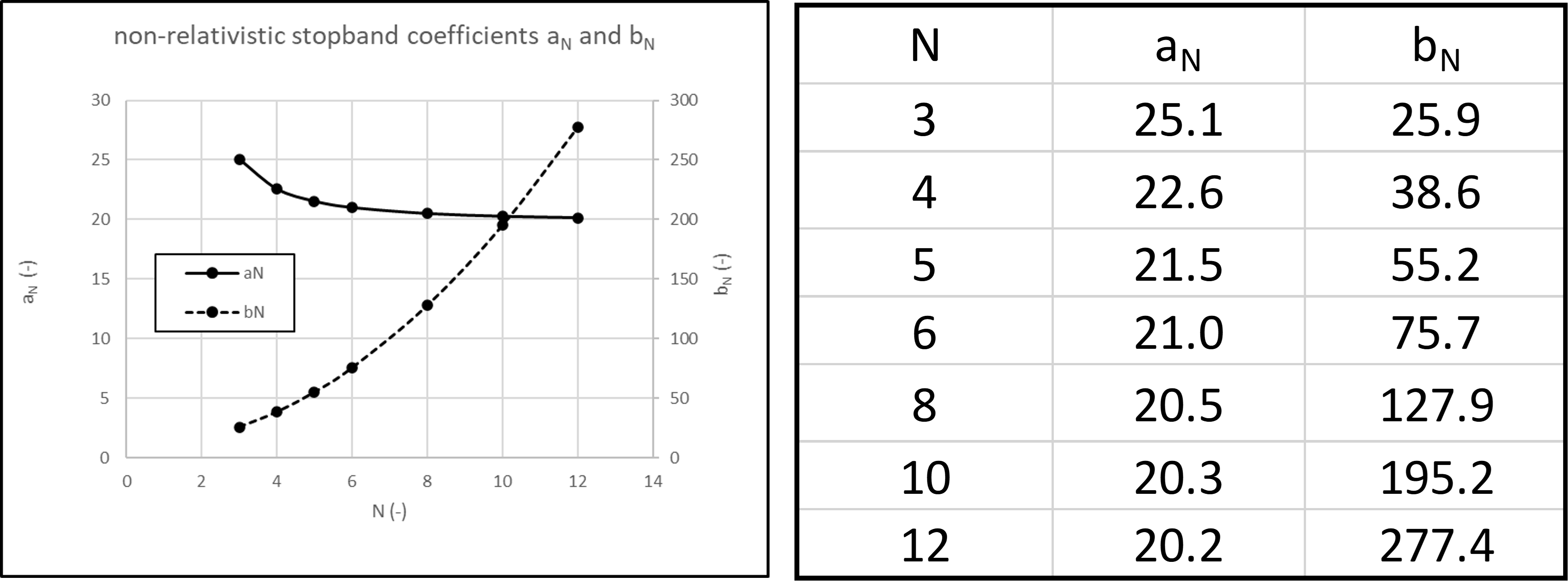
Figure 10: Stopband coefficients for non-relativistic derivation.

Figure 11 shows the impact of three different types of approximation on the calculated limits of the half-integer resonance stopband. The upper two figures show the differences that are due to the non-relativistic model as compared to the relativistic model. Or in other words, the improvement that is obtained by taking into account in the derivations the cross-terms between average field derivatives and the azimuthal field modulation. It is seen that this improvement is considerable, especially for the higher values of cyclotron rotational symmetry number $N$. This may be expected because higher $N$-value corresponds with higher stopband energies and thus higher values of the field-derivatives (see Figure 15). The effect of the resonance is substantially under-estimated for the non-relativistic derivation. The middle two figures show the differences that are due to second order model ($\mathscr{O}(f^{2})$) as compared to the first order model ($\mathscr{O}(f)$). Or in other words, the improvement that is obtained by taking into account terms up to $\mathscr{O}(f^{2})$. It is seen that this improvement is considerable, both for lower $N$-values and higher $N$-values. It is seen that the impact of the resonance is under-estimated if $\mathscr{O}(f^{2})$ terms are ignored.

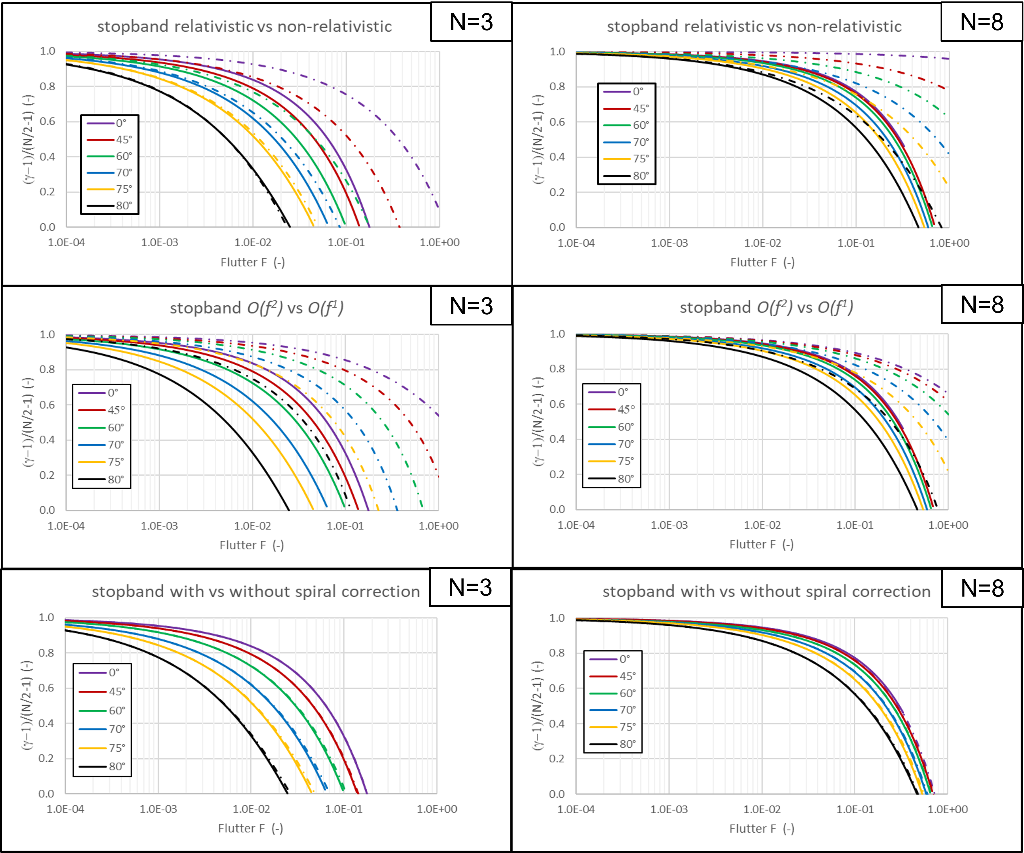
Figure 11: Impact of 3 types of approximations/refinements on the calculated limits of the half-integer resonance stopband

The lower two cases in Figure 11 show the differences that are due to use if the corrected spiral angle. This correction, as discussed in appendix 3.2, allowed for a better agreement between the numerical C400 vertical tune function and the analytical prediction (as shown in Figure 7). However, for the stopband limits this refinement only has a minor impact.

6 Energy limit of an isochronous cyclotron

In the previous paragraph we derived the stability zone of the isochronous cyclotron resulting from the half-integer resonance $2\nu_{r}=N$. It was seen that the stopband lower limit $\gamma_{1}$ can be increased by lowering the flutter $F$ or the sector spiral angle $\varphi^{\prime}$. However in doing so, the vertical tune will decrease and the cyclotron may become vertically unstable. Besides the resonance limit, there is also an energy limit due to lack of vertical focusing. This limit is determined by the condition $\nu_{z}=0$ and can be calculated from Eq. (47) by inserting $\nu_{x}^{2}=0$ and $\bar{\mu}^{\prime}_{rel}=\gamma^{2}-1$. Since the tune coefficients $\hat{a}_{N},\hat{b}_{N}$ also depend on $\gamma$, the resulting equation is an implicit equation for $\gamma$. We solve it by the iterative method of successive substitution. The dominant tune coefficient $\hat{b}_{N}$ depend only weakly on $\gamma$ and thereforeonly a few iterations are needed (a maximum of 4 for the lowest spiral angle of 45°).

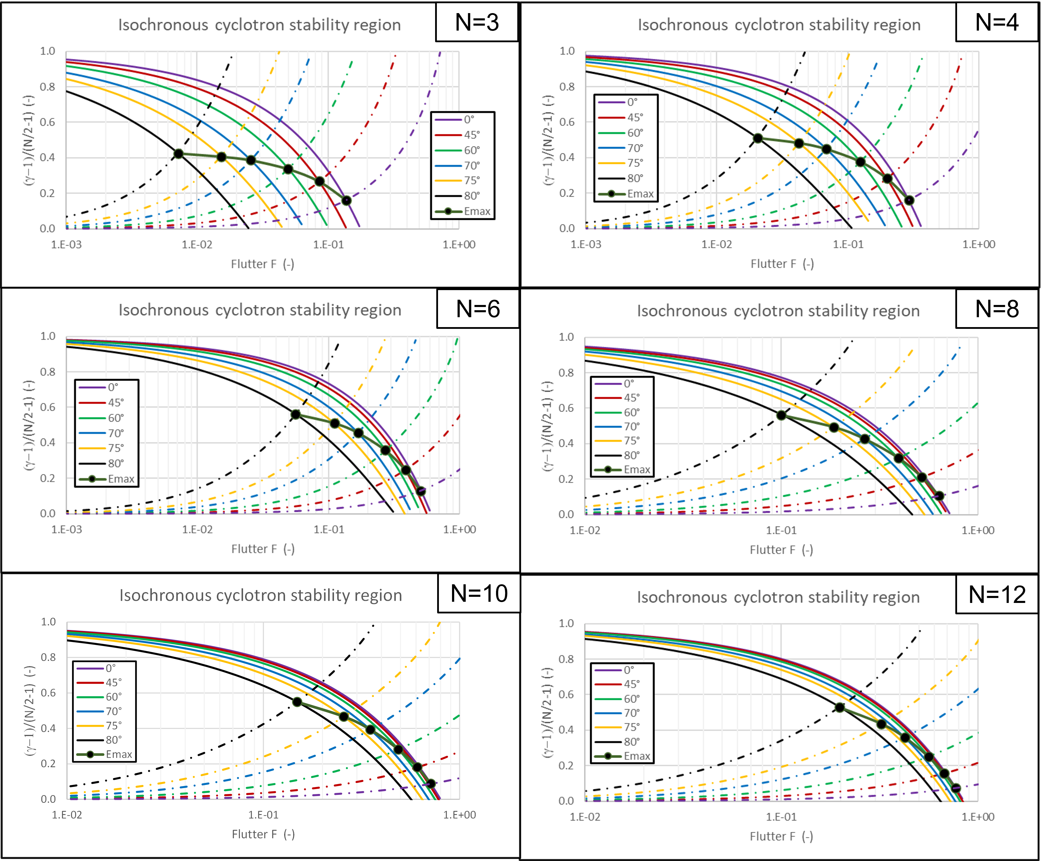
Figure 12: Stability diagram of the isochronous cyclotron

Figure 12 shows in one plot both the resonance limits (solid lines) and the vertical focusing limits (dashed lines) as function of the flutter $F$. The different cases shown and also the axes units are the same as used in Figure 9. It is seen that the focusing limit increases monotonically with increasing flutter and increasing spiral angle. The normalized limit $(\gamma-1)/(\tfrac{N}{2}-1)$ decreases monotonically with increasing N-number. In order to have a stable cyclotron, the operating point as defined by a given flutter, spiral angle and $\gamma$-value must be below the corresponding solid lines and the corresponding dashed lines in Figure  12. It should be remembered that the lines itself represent extreme limits of stability and in practice sufficient distance must be taken. For the vertical tune one could require for example a minimum value $\nu_{min}>0$. In this case the dashed line in the plot will shift down by the amount:

$$\Delta\gamma\approx-\frac{\nu_{min}^{2}}{2\gamma_{0}}\ ,$$ (90)

where $\gamma_{0}$ is the energy limit as given by the dashed line in Figure 12.

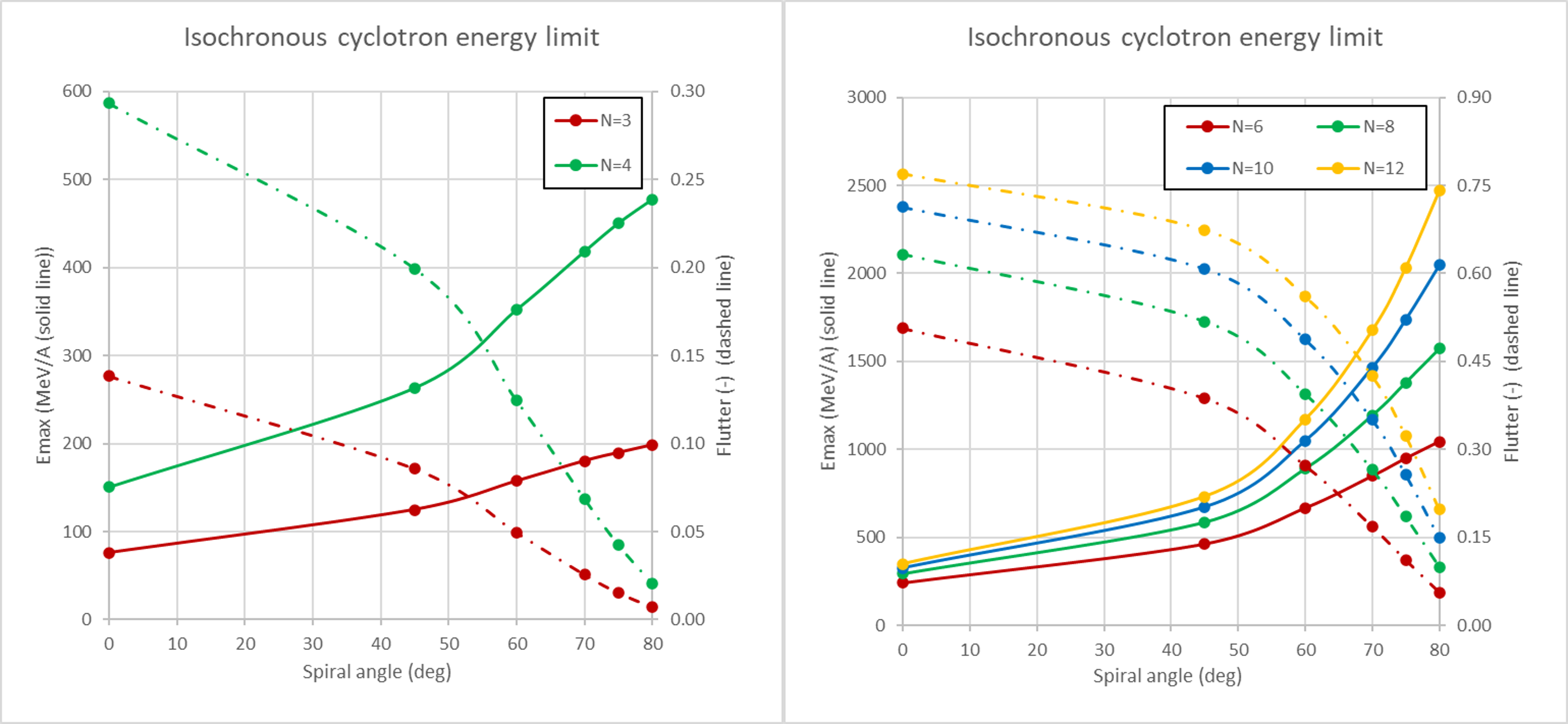
Figure 13: Energy limit of the isochronous cyclotron

Table 1: Energy limits of an isochronous cyclotron

	N=3		N=4		N=6
$\xi$ (deg)	F (-)	T (MeV/u)	F (-)	T (MeV/u)	F (-)	T (MeV/u)
0	0.1384	75.7	0.2934	151	0.5063	243
45	0.0858	125	0.1995	263	0.387	464
60	0.0495	157	0.1245	352	0.272	668
70	0.0257	180	0.0686	418	0.168	850
75	0.0153	190	0.0424	450	0.111	950
80	0.0072	198	0.0204	477	0.056	1045
	N=8		N=10		N=12
0	0.6324	294	0.7135	326	0.7697	348
45	0.5180	587	0.6085	673	0.6741	732
60	0.3945	891	0.4880	1049	0.5607	1170
70	0.2653	1193	0.3510	1465	0.4250	1677
75	0.1852	1380	0.2571	1738	0.3231	2034
80	0.1000	1572	0.1488	2047	0.1975	2471

At the intersection between solid and dashed lines the highest achievable energy is found for a given symmetry number $N$ and a given spiral angle. These points are shown as black dots in Figure 12. Figure 13 shows these energy limits (solid lines) as a function of the design spiral angle and for the same N-numbers as used before. These are kinetic energies expressed in MeV per nucleon. The graphs also show the corresponding flutter values (dashed lines) that are required to achieve these limits. The numerical data are given also in Table 1. The energy limits are the absolute limits for the isochronous cyclotron as dictated by the beam dynamics of these machines. In practice there are of course other limits determined by technology.

Figure 14 shows the tunes for a $H_{2}^{+}$ cyclotron with symmetry N=3, that has been studied at IBA. The left figure shows the radial tune and vertical tune (2x) obtained from a numerical closed orbit code (black-solid and red solid respectively), and also the radial tune (black-dashed) and vertical tune (2x, red-dashed) calculated analytically from Eq. (47) and Eq. (62) respectively. In this example, the half-integer resonance hits at the radius of 48.2 cm, corresponding with an energy of 187.5 MeV/u and a vertical tune value of $\nu_{z}$=0.27. The right figure shows the flutter $F$ and the spiral angle $\xi$ of the magnetic field. At the resonance energy they are F=0.0074 and $\xi$=79.5° respectively. Table 1 shows an extreme energy for $\xi$=80° of 198 MeV/u. Correcting this value for the non-zero vertical tune (=0.27), using Eq. (90), we obtain the stopband energy at E=186.5 MeV/u. This is extremely close to the numerical result of 187.5 MeV/u.

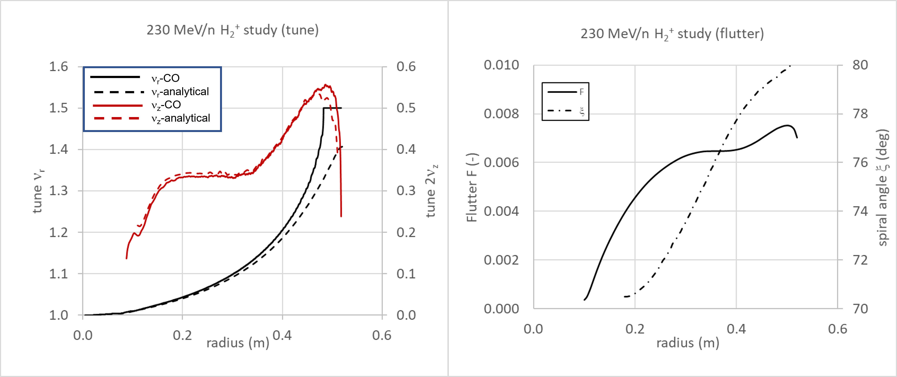
Figure 14: Example for a 230 MeV/u $H_{2}^{+}$ cyclotron.

Appendix A The cyclotron Hamiltonian

We use a polar coordinate system ($\theta,r,z$) that in this sequence is chosen to be right-handed. Then a positively charged particle moves in the positive $\theta$-direction if the average magnetic field, pointing along the z-direction, is positive. The canonical conjugate variables in polar coordinates are:

$$-E\hskip 83.93553pt ;t\ ,$$ (A1)

$$P_{\theta}=mrv_{\theta}+qrA_{\theta} ;\theta\ ,$$ (A2)

$$P_{r}=mv_{r}+qA_{r}\hskip 12.80365pt ;r\ ,$$ (A3)

$$P_{z}=mv_{z}+qA_{z}\hskip 12.80365pt ;z\ .$$ (A4)

Here $E$ is the total energy of the particle, $m$ its relativistic mass, $q$ its charge, ($v_{\theta},v_{r},v_{z}$) the polar velocity components, ($P_{\theta},P_{r},P_{z}$) the canonical momenta and ($A_{\theta},A_{r},A_{z}$) the components of the magnetic vector potential. The magnetic field $\vec{B}$ is obtained from the vector potential via:

$$\vec{B}=\nabla\times\vec{A}\ .$$ (A5)

The kinetic momentum $P_{0}$ of a particle is given by:

$$P_{0}=mv=\sqrt{(P_{\theta}/r-qA_{\theta})^{2}+(P_{r}-qA_{r})^{2}+(P_{z}-qA_{z})^{2}}\ .$$ (A6)

Throughout this paper, we consider the motion in a static magnetic field only (no electric fields). In this case the kinetic momentum $P_{0}$ is a constant of motion. Chosing $\theta$ as the independent variable, the Hamiltionian $\mathscr{H}$ is equal to $-P_{\theta}$. $\mathscr{H}$ can be solved from Eq. (A6) giving:

$$\mathscr{H}=-P_{\theta}=-r\sqrt{P_{0}^{2}-(P_{r}-qA_{r})^{2}+(P_{z}-qA_{z})^{2}}-qrA_{\theta}\ .$$ (A7)

We have some freedom in the choice of $\vec{A}$ and take a potential for which $A_{r}\equiv 0$. The expressions for $A_{\theta}$ and $A_{z}$ then become:

$$A_{\theta}(\theta,r,z) =-\frac{1}{r}\int^{r}r^{\prime}B_{z}(\theta,r^{\prime},z)\,dr^{\prime}\ ,$$ (A8)

$$A_{z}(\theta,r,z) =\int^{r}B_{\theta}(\theta,r^{\prime},z)\,dr^{\prime}\ .$$ (A9)

Its is easily verified with Eq. (A5) and the divergence law $\nabla\cdot\vec{B}=0$ that this definition of the vector potential gives the correct result for all three magnetic field components.

We expand the magnetic field with respect to the $z$-coordinate and assume that the median plane ($z=0$) is a symmetry plane. We get:

$$B_{\theta}(\theta,r,z) =\frac{z}{r}\frac{\partial B}{\partial\theta}+\mathscr{O}(z^{3})\ ,$$ (A10)

$$B_{r}(\theta,r,z) =z\frac{\partial B}{\partial r}+\mathscr{O}(z^{3})\ ,$$ (A11)

$$B_{z}(\theta,r,z) =B(\theta,r)-\frac{1}{2}z^{2}\Delta B(\theta,r)+\mathscr{O}(z^{4})\ .$$ (A12)

Here $B(\theta,r)=B_{z}(\theta,r,0)$ is the median plane field and $\Delta B$ is the 2D laplacian of $B$ in the median plane:

$$\Delta B(\theta,r)=\frac{1}{r\partial r}(r\frac{\partial B}{\partial r})+\frac{1}{r^{2}}\frac{\partial^{2}B}{\partial\theta^{2}}\ .$$ (A13)

In our development of the Hamiltonian we neglect terms that envolve vertical phase space variables of higher than quadratic degree. With this simplification, the final Hamiltonian describes linear vertical motion. For the radial motion no such simplification is made. Almost throughout this paper the motion of the particle is analyzed in the neighborhood of a circle with radius $r_{0}$, where $r_{0}$ is related to the constant momentum $P_{0}$ of the particle via:

$$P_{0}=qr_{0}\bar{B}(r_{0})\ .$$ (A14)

Here $\bar{B}$ is the average magnetic field around the circle. In order to facilitate the analysis, we introduce new reduced variables with the following normalizations:

$$x=\frac{r-r_{0}}{r_{0}} ;\hskip 28.45274pt\tilde{p}_{x}=\frac{P_{r}}{P_{0}}\ ,$$ (A15)

$$\zeta=\frac{z}{r_{0}}\hskip 19.91684pt ;\hskip 28.45274pt\tilde{p}_{z}=\frac{P_{z}}{P_{0}}\ .$$ (A16)

The Hamiltonian must be adjusted accordingly; using Eqs. (G7,G8) we find for the new Hamiltonian:

$$\mathscr{K}=\frac{\mathscr{H}}{r_{0}P_{0}}\ .$$ (A17)

We also define the reduced median plane magnetic field $\mu$ (around $r_{0}$) as follows:

$$\mu(\theta,r)=\frac{B(\theta,r)}{\bar{B}(r_{0})}=\frac{B(\theta,r_{0}+r_{0}x)}{\bar{B}(r_{0})}\ .$$ (A18)

With this normalization the vector potential terms in Eq. (A7) become:

$$rA_{\theta} =-r_{0}^{2}\bar{B}(r_{0})\left[\int^{x}(1+x^{\prime})\mu(\theta,x^{\prime})\,dx^{\prime}-\frac{1}{2}\zeta^{2}\left((1+x)\frac{\partial\mu}{\partial x}+\int^{x}\frac{1}{1+x^{\prime}}\frac{\partial^{2}\mu}{\partial\theta^{2}}dx^{\prime}\right)\right]\ ,$$ (A19)

$$A_{z} =r_{0}\bar{B}(r_{0})\zeta\int^{x}\frac{1}{1+x^{\prime}}\frac{\partial\mu}{\partial\theta}dx^{\prime}\ .$$ (A20)

Inserting these expressions into Eq. (A7) and applying the normalizations defined in Eqs. (A14-A17) we find for the new Hamiltonian:

$$\mathscr{K}= -(1+x)\sqrt{1-\tilde{p}_{x}^{2}-\left(\tilde{p}_{z}-\zeta\int^{x}\frac{1}{1+x^{\prime}}\frac{\partial\mu}{\partial\theta}dx^{\prime}\right)^{2}}$$ (A21)

$$+\int^{x}(1+x^{\prime})\mu(\theta,x^{\prime})\,dx^{\prime}-\frac{1}{2}\zeta^{2}\left((1+x)\frac{\partial\mu}{\partial x}+\int^{x}\frac{1}{1+x^{\prime}}\frac{\partial^{2}\mu}{\partial\theta^{2}dx^{\prime}}\right)\ .$$

Due to our choice of the vector potential the radial canonical momentum $P_{r}$ is equal to the radial kinetic momentum $mv_{r}$ and therefore the normalized momentum $\tilde{p}_{x}$ is equal to the radial divergence of the particle. In order to obtain the same interpretation for the vertical momentum, we apply a canonical transformation. We use a type 2 generating function that depends on the original coordinates $x,\zeta$ and the new momenta $p_{x},p_{z}$ (see Eq. (G10)):

$$G_{2}(x,\zeta,p_{x},p_{z})=xp_{x}+\zeta p_{z}+\frac{1}{2}\zeta^{2}\int^{x}\frac{1}{1+x^{\prime}}\frac{\partial\mu}{\partial\theta}dx^{\prime}\ ,$$ (A22)

$$\tilde{p}_{x}=\frac{\partial G_{2}}{\partial x}=p_{x}+\frac{\zeta^{2}}{2(1+x)}\frac{\partial\mu}{\partial\theta}\ ,$$ (A23)

$$\tilde{p}_{z}=\frac{\partial G_{2}}{\partial\zeta}=p_{z}+\zeta\int^{x}\frac{1}{1+x^{\prime}}\frac{\partial\mu}{\partial\theta}dx^{\prime}\ ,$$ (A24)

$$\frac{\partial G_{2}}{\partial\theta}=\frac{1}{2}\zeta^{2}\int^{x}\frac{1}{1+x^{\prime}}\frac{\partial^{2}\mu}{\partial\theta^{2}}dx^{\prime}\ .$$ (A25)

Keeping terms up to quadratic degree in $\zeta,p_{z}$, we obtain for the new Hamiltonian:

$$\bar{\mathscr{K}}=-(1+x)\sqrt{1-p_{x}^{2}-p_{x}\frac{\zeta^{2}}{1+x}\frac{\partial\mu}{\partial\theta}-p_{z}^{2}}+\int^{x}(1+x^{\prime})\mu(\theta,x^{\prime})dx^{\prime}-\frac{\zeta^{2}}{2}(1+x)\frac{\partial\mu}{\partial x}\ .$$ (A26)

We expand this Hamiltonian with respect to the vertical phase space variables and keep terms up to quadratic degree in $\zeta,p_{z}$. This gives:

$$\bar{\mathscr{K}}=-(1+x)(1-p_{x}^{2})^{1/2}+\int^{x}(1+x^{\prime})\mu(\theta,x^{\prime})dx^{\prime}\hskip 56.9055pt$$ (A27)

$$+\frac{(1+x)}{2\sqrt{1-p_{x}^{2}}}p_{z}^{2}+\frac{1}{2}\left(\frac{p_{x}}{\sqrt{1-p_{x}^{2}}}\frac{\partial\mu}{\partial\theta}-(1+x)\frac{\partial\mu}{\partial x}\right)\zeta^{2}\ .$$ (A28)

Since we have assumed a symmetric median plane, $\zeta=p_{z}=0$ is a valid solution of Eq. (A27). For this solution we can define the 2D Hamiltonian $H_{x}$ describing the median plane radial motion; it is given by:

$$\boxed{H_{x}=-(1+x)(1-p_{x}^{2})^{1/2}+\int^{x}(1+x^{\prime})\mu(\theta,x^{\prime})\,dx^{\prime}\ .}$$ (A29)

If at the same time the vertical excursion from the median plane $\zeta$ is small, the influence of the vertical motion on the radial motion is negligible, and we may consider $x,p_{x}$ as given functions of $\theta$ and define the 2D Hamiltonian $H_{z}$ for the vertical motion.

$$\boxed{H_{z}=\frac{(1+x)}{2\sqrt{1-p_{x}^{2}}}p_{z}^{2}+\frac{1}{2}\left(\frac{p_{x}}{\sqrt{1-p_{x}^{2}}}\frac{\partial\mu}{\partial\theta}-(1+x)\frac{\partial\mu}{\partial x}\right)\zeta^{2}\ }.$$ (A30)

The equations (A29) for $H_{x}$ and (A30) for $H_{z}$ agree with respectively Eq. (4.3) and Eq. (10.2) in the Hagedoorn-Verster paper[3].

Appendix B The median plane magnetic field

The motion of the particle is dertemined by the shape of the median plane magnetic field $B(\theta,r)$. This field can be separated in an average part $\bar{B}(r)$ and an oscillating part. This part represents the azimuthal variation of the field which we exand in a Fourier series. We write $B(\theta,r)$ as:

$$B(\theta,r)=\bar{B}(r)+\operatorname*{\textstyle\sum}_{n}\mathscr{A}_{n}(r)\cos n\theta+\mathscr{B}_{n}(r)\sin n\theta.$$ (B1)

In our analysis we assume that the cyclotron has perfect $N$-fold symmetry. In this case only terms with $n=kN,k=1,2,\dots$ will be present in the Fourier series.

B.1 The reduced magnetic field

In this paper we analyze the orbits in the vincinity of a circle with radius $r_{0}$ (see Eq. (A14)) and define the reduced magnetic field $\mu$ (around $r_{0}$) as follows:

$$\mu(\theta,r)=\frac{B(\theta,r)}{\bar{B}(r_{0})}=\frac{B(\theta,r_{0}+r_{0}x)}{\bar{B}(r_{0})}\ .$$ (B2)

Here $x$ has been defined in Eq. (A15).

Using Eqs. (B1,B2), we can write the reduced field as:

$$\mu(\theta,r)=\bar{\mu}(r)+f(\theta,r)\ ,$$ (B3)

where $\bar{\mu}(r)$ and $f(\theta,r)$ are defined as :

$$\bar{\mu}(r) =\bar{B}(r)/\bar{B}(r_{0})\ ,$$ (B4)

$$f(\theta,r) =\operatorname*{\textstyle\sum}_{n}A_{n}(r)\cos n\theta+B_{n}(r)\sin n\theta\ ,$$ (B5)

and with:

$$A_{n}(r)=\mathscr{A}_{n}(r)/\bar{B}(r_{0})\ ,\hskip 14.22636ptB_{n}(r)=\mathscr{B}_{n}(r)/\bar{B}(r_{0})\ .$$ (B6)

The Fourier series in Eq. (B5) can also be written in terms of amplitude and phase of the harmonics as:

$$f(\theta,r)=\operatorname*{\textstyle\sum}_{n}C_{n}(r)\cos n(\theta-\varphi_{n}(r))\ ,$$ (B7)

where $C_{n},\varphi_{n}$ relate to $A_{n},B_{n}$ as:

$$A_{n}(r) =C_{n}(r)\cos\varphi_{n}\ ,$$ (B8)

$$B_{n}(r) =C_{n}(r)\sin\varphi_{n}\ ,$$ (B9)

We expand the reduced field $\mu(\theta,x)$ in a taylor series:

$$\mu(\theta,x) =1+\bar{\mu}^{\prime}x+\tfrac{1}{2}\bar{\mu}^{\prime\prime}x^{2}+\tfrac{1}{6}\bar{\mu}^{\prime\prime\prime}x^{3}+\dots$$

$$+\operatorname*{\textstyle\sum}_{n}(A_{n}+A_{n}^{\prime}x+\tfrac{1}{2}A_{n}^{\prime\prime}x^{2}+\dots)\cos n\theta$$

$$+\operatorname*{\textstyle\sum}_{n}(B_{n}+B_{n}^{\prime}x+\tfrac{1}{2}B_{n}^{\prime\prime}x^{2}+\dots)\sin n\theta\ ,$$ (B10)

where:

$$\bar{\mu}^{\prime} =\left[\frac{d}{dx}\bar{\mu}(r_{0}+r_{0}x)\right]_{x=0}\hskip 11.38092pt=\left[\frac{r}{\bar{B}}\frac{d\bar{B}}{dr}\right]_{r=r_{0}}\ ,$$

$$\bar{\mu}^{\prime\prime} =\left[\frac{d^{2}}{dx^{2}}\bar{\mu}(r_{0}+r_{0}x)\right]_{x=0}\hskip 7.96674pt=\left[\frac{r^{2}}{\bar{B}}\frac{d^{2}\bar{B}}{dr^{2}}\right]_{r=r_{0}}\ ,$$

$$A_{n} =A_{n}(r_{0})\hskip 79.6678pt=\hskip 96.73918pt=\left[\frac{a_{n}(r)}{\bar{B}(r)}\right]_{r=r_{0}}\ ,$$ (B11)

$$A_{n}^{\prime} =\left[\frac{d}{dx}A_{n}(r_{0}+r_{0}x)\right]_{x=0}\hskip 5.12128pt=\left[r\frac{d}{dr}A_{n}(r)\right]_{r=r_{0}}\hskip 8.5359pt=\left[\frac{r}{\bar{B}}\frac{da_{n}}{dr}\right]_{r=r_{0}}\ ,$$

$$A_{n}^{\prime\prime} =\left[\frac{d^{2}}{dx^{2}}A_{n}(r_{0}+r_{0}x)\right]_{x=0}=\left[r^{2}\frac{d}{dr^{2}}A_{n}(r)\right]_{r=r_{0}}=\left[\frac{r^{2}}{\bar{B}}\frac{d^{2}a_{n}}{dr^{2}}\right]_{r=r_{0}}\ ,$$

As an important remark, we note that our definition of the field-harmonics differs with a factor $\bar{B}(r)/\bar{B}(r_{0})$ from the definition used in the HV-paper[3]. The relation between our representation $A_{n}$ and the HV-representation $\tilde{A}_{n}$is as follows:

$$A_{n}=\tfrac{\bar{B}(r)}{\bar{B}(r_{0})}\tilde{A}_{n}\ ,$$

$$A_{n}(r_{0})=\tilde{A}_{n}(r_{0})\ ,$$ (B12)

$$A_{n}^{\prime}=\tilde{A}_{n}^{\prime}+\bar{\mu}^{\prime}\tilde{A}_{n}\ ,$$

$$A_{n}^{\prime\prime}=\tilde{A}_{n}^{\prime\prime}+2\bar{\mu}^{\prime}\tilde{A}_{n}^{\prime}+\bar{\mu}^{\prime\prime}\tilde{A}_{n}\ ,$$

and similar equations for the sine-components.

The advantage of our definition is that in the Taylor development (Eq. (B10)), there are no cross-terms between derivatives of the average field and the Fourier components. In the HV-approach, there are such cross-terms, but they have been neglected from the beginning. They were neglected not only in the magnetic field development but at all developments throughout their paper, with the argument that the average field dervatives are very small ($\mathscr{O}(f^{2})$. and crossterms therefore are small up to $\mathscr{O}(f^{3})$. This is true for not too high particle energies but it becomes less and less valid for more relativistic energies. Figure 15 shows quantities $\bar{\mu}^{\prime},\bar{\mu}^{\prime\prime}$ and $\bar{\mu}^{\prime\prime\prime}$ as a function of the relativistic parameter $\gamma-1$. The value $\gamma-1=0.5$ corresponds with a kinetic energy of about 470 MeV/A. It is seen that at this energy $\bar{\mu}^{\prime}\approx 1.2$, $\bar{\mu}^{\prime\prime}\approx 6$ and $\bar{\mu}^{\prime\prime\prime}\approx 43$. Since in our study we are interested in the optics and stability at higher energies, we consider the derivative as functions of $\mathscr{O}(f^{0})$ and therefore do not neglect the cross-terms at any moment in our development.

Figure 15: Normalized first and second derivatives (left scale) and third derivative (right scale) of an isochronous magnetic field.

B.2 Relations between magnetic field Fourier components

Several times in our analysis we need to transform expressions using the sine/cosine representation of the azimuthal field variation into expressions using the amplitude/phase representation. For such transformations we use the following relations:

$$A^{2}_{n}+B^{2}_{n}=C^{2}_{n}\ ,$$ (B13)

$$A_{n}A_{n}^{\prime}+B_{n}B_{n}^{\prime}=C_{n}C_{n}^{\prime}\ ,$$ (B14)

$$A_{n}^{\prime 2}+B_{n}^{\prime 2}=C_{n}^{\prime 2}+n^{2}C_{n}^{2}\varphi_{n}^{\prime 2}\ ,$$ (B15)

$$A_{n}A_{n}^{\prime\prime}+B_{n}B_{n}^{\prime\prime}=C_{n}^{\prime 2}-n^{2}C_{n}^{2}\varphi_{n}^{\prime 2}\ .$$ (B16)

Here $C_{n}^{\prime},\varphi_{n}^{\prime}$ are defined as shown in Eqs. (B11), for $A_{n}^{\prime}$.

B.3 The spiral angle

Note that $\varphi^{\prime}_{n}$ is related to the frequentlly used spiral angle $\xi_{n}$ as follows:

$$\varphi_{n}^{\prime}=\tan\xi_{n}\ .$$ (B17)

If $\theta=\varphi_{n}(r)$ is the contour where the n${}^{\mbox{th}}$ Fourier component is maximum, then the spiral at a given point on this contour is defined as the angle between a radial unit vector (the vector $\vec{n}$ normal to the circle) and the tangent along the contour. In practice one often uses for $\varphi$ the contour of the entrance or exit pole edge of the sector, or the contour of the mid-sector angle. This is illustrated in Figure 16.

Figure 16: Definition of the spiral angle.

B.4 Relations between Fourier harmonics and flutter

In our analysis of cyclotron optics whe derive equations for optical quantities (such as the tunes for example) that depend on (summations over $n$ of) the Fourier harmonics and their derivatives and on the derivatives of the average magnetic field. These are rather complex and also impractical equations. In order to simpify them we look for away to relate the higher Fourier harmonics $(n>N)$ to the principal harmonics $(n=N)$. This envolves some approximation which however is not so significant because the optical quantities are dominantly determined by the principal harmonics and less by the higher harmonics. Making some error in the values of the higher harmonics therefore does not have a too big impact. It will lead us however to more pratical forms of the equations. In order to make such an approximation, we assume a hard-edge profile of the azimuthal field variation. In this case the relation between the higher harmonic amplitudes $C_{kN}$ and the principal harmonic amplitude $C_{N}$ is given by:

$$C_{kN}=\frac{\sin(kN\alpha_{h})}{k\sin(N\alpha_{h})}C_{N}\ ,\hskip 56.9055ptk=1,2,\dots\ ,$$ (B18)

where $\alpha_{h}$ is half of the hill angular extend.

We simplify a little bit more by assuming a symmetric structure where the hill angle is equal to the valley angle. In this case only Fourier components with $n=N,3N,5N,\dots\ ,$ are non-zero and we get:

$$C_{(2k+1)N}=\frac{C_{N}}{2k+1}(-1)^{k}\hskip 56.9055pt\mbox{for}\ k=0,1,2,\dots\ ,$$ (B19)

We can also make the relation with the frequently used flutter of the magnetic field. The flutter is defined by the equation:

$$F(r)=\frac{{{\langle}}B^{2}(\theta,r){{\rangle}}-{{\langle}}B(\theta,r){{\rangle}}^{2}}{{{\langle}}B(\theta,r){{\rangle}}^{2}}\ ,$$ (B20)

and can be expressed in the Fourier components:

$$F(r)=\tfrac{1}{2}\operatorname*{\textstyle\sum}_{n}[A^{2}_{n}(r)+B^{2}_{n}(r)]=\tfrac{1}{2}\operatorname*{\textstyle\sum}_{n}C^{2}_{n}(r)\ .$$ (B21)

Inserting in this expression for $F$ the Fourier components defined in Eq. (B19) and choosing the summation coefficient as $n=(2k+1)N$ we get:

$$F=\tfrac{1}{2}C_{N}^{2}\operatorname*{\textstyle\sum}_{k=0}^{\infty}\frac{1}{(2k+1)^{2}}\ .$$ (B22)

The series in the above equation is one of the Leonard Euler series:

$$\operatorname*{\textstyle\sum}_{k=0}^{\infty}\frac{1}{(2k+1)^{2}}=\frac{\pi^{2}}{8}\ ,$$ (B23)

and with this we get:

$$F=\frac{\pi^{2}}{16}C_{N}^{2}\ .$$ (B24)

For use elsewhere in this report, we now give the following relations between the Flutter $F$ and the (square of) the Fourier amplitudes $C_{n}$:

$$\ C_{n}^{2} =\frac{N^{2}}{n^{2}}C_{N}^{2} =\frac{16F}{\pi^{2}(2k+1)^{2}}\ ,$$ (B25)

$$\ C_{n}C_{n}^{\prime} =\frac{N^{2}}{n^{2}}C_{N}C_{N}^{\prime} =\frac{8F^{\prime}}{\pi^{2}(2k+1)^{2}}\ ,$$

$$\ C_{n}^{\prime 2} =\frac{N^{2}}{n^{2}}C_{N}^{\prime 2} =\frac{4F^{\prime 2}/F}{\pi^{2}(2k+1)^{2}}\ ,$$

$$\ C_{n}C_{n}^{\prime\prime} =\frac{N^{2}}{n^{2}}C_{N}C_{N}^{\prime\prime} =\frac{8(F^{\prime}+F^{\prime\prime}-F^{\prime 2}/2F)}{\pi^{2}(2k+1)^{2}}\ .$$

In the right hand side of these equations we replaced $n$ by $(2k+1)N$.

Appendix C Move an oscillating term to the next higher order

Consider a Hamiltonian of the following form:

$$H(p,x,\theta)=\tfrac{1}{2}p^{2}+\tfrac{1}{2}(\nu_{0}^{2}+f(\theta))x^{2}\ .$$ (C1)

Here we assume the function $f$ to be an oscillating function ($\langle f\rangle=0$) with a small oscillating amplitude. The parameter $\nu_{0}$ may be considered as the zero-order tune of the oscillation. We want to design a canonical transformation which removes the function $f$ from the Hamiltonian up to first order $\mathscr{O}(f)$. The new Hamiltonian may have oscillating terms of $\mathscr{O}(f^{2})$, which we consider small enough to be negligible. We will keep constant ($\theta$-independent) terms up to $\mathscr{O}(f^{2})$. When this has been achieved the motion is solved (up to $\mathscr{O}(f^{2})$) as the Hamiltonian has become a constant. We note that the transformation has been given in the HV-paper[3], but only for the case where $\nu_{0}^{2}$ itself is also a small quentity of $\mathscr{O}(f^{2})$. In our cases of interest, this is not always true and therefore we generalize the transformation. We write for the generating function:

$$G=G_{3}(p,\bar{x})=-p\bar{x}+\tfrac{1}{2}a(\theta)\bar{x}^{2}+b(\theta)\bar{x}p+\tfrac{1}{2}c(\theta)p^{2}\ ,$$ (C2)

where $a(\theta),b(\theta),c(\theta)$ are yet unknown periodic functions. They will be dertermined by requiring that in the new Hamiltonian $\bar{H}$, the $\mathscr{O}(f)$ oscillating part is removed. For that purpose we first carry out the transformation up to $\mathscr{O}(f)$. We obtain from the above generating function:

$$x = -\frac{\partial G_{3}}{\partial p}=\bar{x}-b\bar{x}-cp\ ,$$

$$\bar{p} = -\frac{\partial G_{3}}{\partial\bar{x}}=p-a\bar{x}-bp\ ,$$

$$\frac{\partial G_{3}}{\partial\theta} = +\tfrac{1}{2}\dot{a}\bar{x}^{2}+\dot{b}\bar{x}p+\tfrac{1}{2}\dot{c}p^{2}\ .$$

Up to first order $\mathscr{O}(f)$, we obtain for the new Hamiltonian:

$$\bar{H}=\tfrac{1}{2}(1+2b+\dot{c})\bar{p}^{2}+(a-\nu_{0}^{2}c+\dot{b})\bar{x}\bar{p}+\tfrac{1}{2}(\nu_{0}^{2}-2b\nu_{0}^{2}+f+\dot{a})\bar{x}^{2}\ .$$ (C3)

For all first order terms to be zero, the functions $a,b,c$ must obey the following relations:

$$4\nu_{0}^{2}\dot{c}+\dddot{c} = -2f(\theta)\ ,$$ (C4)

$$b = -\tfrac{1}{2}\dot{c}\ ,$$ (C5)

$$a = \nu_{0}^{2}c+\tfrac{1}{2}\ddot{c}\ .$$ (C6)

We now carry out the transformation Eq (C2) up to second order ($\mathscr{O}(f^{2})$). In this approximation we get the following relations:

$$x = (1-b-ac)\bar{x}-c(1+b)\bar{p}\ ,$$

$$p = a(1+b)\bar{x}+(1+b+b^{2})\bar{p}\ ,$$

$$\tfrac{\partial G_{3}}{d\theta} = \tfrac{1}{2}\dot{a}\bar{x}^{2}+\dot{b}\bar{x}(\bar{p}+a\bar{x}+b\bar{p})+\tfrac{1}{2}\dot{c}(\bar{p}^{2}+2a\bar{x}\bar{p}+2b\bar{p}^{2})\ ,$$

and find for the new Hamiltonian:

$$\bar{H}=\tfrac{1}{2}(1+3b^{2}+\nu_{0}^{2}c^{2}+2b\dot{c})\bar{p}^{2}+\tfrac{1}{2}\left[a^{2}+\nu_{0}^{2}(1+b^{2}-2ac)-2bf+2a\dot{b}\right]\bar{x}^{2}\ .$$ (C7)

We bring this Hamiltonian to its normal form using the method explained in Appendix G.4. We find:

$$\bar{H}=\tfrac{1}{2}\bar{p}^{2}+\tfrac{1}{2}\bar{x}^{2}\left[\nu_{0}^{2}+a^{2}-2bf+2a\dot{b}+\nu_{0}^{2}(b^{2}-2ac+3b^{2}+\nu_{0}^{2}c^{2}+2b\dot{c})\right]\ .$$ (C8)

We insert the expressions for a and b from Eqs. (C5,C6) and get:

$$\bar{H}=\tfrac{1}{2}\bar{p}^{2}+\tfrac{1}{2}(\nu_{0}^{2}-\tfrac{1}{4}\ddot{c}^{2}-\nu_{0}^{2}c\ddot{c}+\dot{c}f)\bar{x}^{2}\ .$$ (C9)

We use the differential equation for $c$ (Eq. (C4)) and apply partial integration to re-write $c\ddot{c}=-\dot{c}^{2}$ and $\dot{c}\dddot{c}=-\ddot{c}^{2}$ and obtain for the Hamiltonian:

$$\bar{H}=\tfrac{1}{2}\bar{p}^{2}+\tfrac{1}{2}\left[\nu_{0}^{2}+\tfrac{1}{2}\langle\dot{c}f\rangle\right]$$ (C10)

Here we only kept the average part of the second order terms and neglected their oscillating parts.

The function $f$ is periodic in $\theta$ and can be expanded into a Fourier series:

$$f(\theta)=\operatorname*{\textstyle\sum}_{n=1}^{\infty}a_{n}\cos n\theta+b_{n}\sin n\theta\ .$$ (C11)

Inserting this expression in Eq. (C4), we can solve for the periodic solution of the function $c$. For $\dot{c}$ we obtain:

$$\dot{c}(\theta)=2\operatorname*{\textstyle\sum}_{n=1}^{\infty}\frac{a_{n}\cos n\theta+b_{n}\sin n\theta}{n^{2}-4\nu_{0}^{2}}\ .$$ (C12)

and our final Hamiltonian becomes:

$$\bar{H}=\tfrac{1}{2}\bar{p}^{2}+\tfrac{1}{2}[\nu_{0}^{2}+\tfrac{1}{2}\operatorname*{\textstyle\sum}_{n=1}^{\infty}\frac{c_{n}^{2}}{n^{2}-4\nu_{0}^{2}}]\bar{x}^{2}\ .$$ (C13)

where $c_{n}$ is the amplitude of the n${}^{\mbox{th}}$ Fourier component:

$$c_{n}=\sqrt{a_{n}^{2}+b_{n}^{2}}\ .$$ (C14)

The Hamiltonian does not depend on $\theta$ anymore and therefore the motion can be considered as solved. The square of the tune $\nu_{x}$ of the motion is given by:

$$\boxed{\nu_{x}^{2}=\nu_{0}^{2}+\tfrac{1}{2}\operatorname*{\textstyle\sum}_{n=1}^{\infty}\frac{c_{n}^{2}}{n^{2}-4\nu_{0}^{2}}\ .}$$ (C15)

In paragraphs 3 and 4 we use the above results to find the vertical and radial tunes of the isochronous cyclotron.

It is seen that if the zero-order tune $\nu_{0}$ aproaches the value of $n/2$, the tune $\nu_{x}$ diverges to infinity. This is a case where the motion dynamics is close to the half-integer resonance. In that case the Hamiltonian of Eq. (C13) does no longer describe the motion correctly. In the next paragraph this special case will be analyzed in more detail.

Appendix D The half-integer resonance

We consider again the Hamiltonian of the form as given in Eq. (C1):

$$H(p,x,\theta)=\tfrac{1}{2}p^{2}+\tfrac{1}{2}[\nu_{0}^{2}+f(\theta)]x^{2}\ .$$ (D1)

where as before the function $f$ is an oscillating function ($\langle f\rangle=0$) with a small oscillating amplitude and parameter $\nu_{0}$ is the zero-order tune of the oscillation. We now study this motion in a different (more general) way such that the result is also valid when the zero-order tune is close to a half-integer $\nu_{0}\approx n/2$. Hereto we introduce action-angle variables $I,\phi$ in a rotating phase space:

$$p = \sqrt{2I\nu_{0}}\sin(\phi-k\theta)\ ,$$ (D2)

$$x = \sqrt{2I/\nu_{0}}\cos(\phi-k\theta)\ .$$ (D3)

Here $\phi$ plays the role of new momentum and $I$ the role of new coordinate. The parameter $k$ is an integer or a half-integer. We are especially interested in the case $k=N/2$, where $N$ is symmetry number of the periodic function $f$. But for comparisson with the previous paragraph C we also allow the values $k=0$ and $k=1$. The canonical transformation is obtained from the following type-2 generating function:

$$G =G_{3}(x,\phi)=\tfrac{1}{2}\nu_{0}x^{2}\tan(\phi-k\theta)\ ,$$ (D4)

$$\frac{\partial G_{3}}{\partial\theta} =-\tfrac{1}{2}\frac{k\nu_{0}x^{2}}{\cos^{2}(\phi-k\theta)}=-kI\ ,$$ (D5)

and the new Hamiltonian becomes:

$$K(\phi,I,\theta)=I[\nu_{0}-k+\frac{f(\theta)}{\nu_{0}}\cos^{2}(\phi-k\theta)]\ .$$ (D6)

We write this Hamiltonian in the following form:

$$K(\phi,I,\theta)=I[a(\phi)+f_{2}(\phi,\theta)]\,.$$ (D7)

where $a(\phi)$ and $f_{2}(\phi,\theta)$ are defined as:

$$a(\phi) = a_{0}+\frac{1}{\nu_{0}}{\langle}f(\theta)\cos^{2}(\phi-k\theta){\rangle}\ ,$$ (D8)

$$f_{2}(\phi,\theta) = \frac{1}{\nu_{0}}\mbox{osc}(f(\theta)\cos^{2}(\phi-k\theta))\ ,$$ (D9)

$$a_{0} = \nu_{0}-k\ .$$ (D10)

We want to design a canonical transformation which removes the oscillating function $f_{2}$ from the Hamiltonian up to first order $\mathscr{O}(f)$. The new Hamiltonian may have oscillating terms of $\mathscr{O}(f^{2})$, which we consider small enough to be negligible. We will keep constant ($\theta$-independent) terms up to $\mathscr{O}(f^{2})$. When this has been achieved the motion is solved (up to $\mathscr{O}(f^{2})$) as the Hamiltonian has become a constant. We note that the transformation has been given in the HV-paper[3], but only for the case where $a$ itself is also a small quantity of $\mathscr{O}(f^{2})$. In our cases of interest, this is not true and therefore we generalize the transformation. We write for the generating function:

$$G = G_{3}(\phi,\bar{I})=-\bar{I}[\phi+U_{2}(\phi,\theta)]\ ,$$

$$I = -\frac{\partial G}{\partial\phi}=\bar{I}(1+\frac{\partial U_{2}}{\partial\phi})\ ,$$

$$\bar{\phi} = -\frac{\partial G}{\partial\bar{I}}=\phi+U_{2}(\phi,\theta)\ ,$$

$$\tfrac{\partial G_{3}}{d\theta} = -\frac{\partial U_{2}}{\partial\theta}\ .$$

Here $U_{2}$ is a yet unknown periodic function which will be dertermined by requiring that in the new Hamiltonian $\bar{K}$, the $\mathscr{O}(f)$ oscillating part is removed. We first calculate $\bar{K}$ as afunction of $\bar{I}$ and the old momentum $\phi$:

$$\bar{K}=\bar{I}[a(\phi)+f_{2}(\phi,\theta)+a\frac{\partial U_{2}}{\partial\phi}+f_{2}\frac{\partial U_{2}}{\partial\phi}-\frac{\partial U_{2}}{\partial\theta}]\ .$$ (D11)

So, in order to remove the first order oscillating part $f_{2}$ from the Hamiltonian, we must define $U_{2}$ by the following equation:

$$\frac{\partial U_{2}}{\partial\theta}-a_{0}\frac{\partial U_{2}}{\partial\phi}=f_{2}(\phi,\theta)\ .$$ (D12)

Note that here we have replaced $a$ by $a_{0}$, because the difference generates an oscillating term of $\mathscr{O}(f^{2})$, which we neglect. With the same reasoning we can (now that the first order part has been removed) replace in Eq. (D11) $\phi$ by $\bar{\phi}$. We get for the final Hamiltonian the following form:

$$\bar{K}=\bar{I}[a(\bar{\phi})+{{\langle}}f_{2}\frac{\partial U_{2}}{\partial\bar{\phi}}{{\rangle}}]\ .$$ (D13)

In order to elaborate this expression furher, we need to find the expressions for $a(\phi)$ and $f_{2}(\phi,\theta))$ and then solve $U_{2}$ from Eq. (D12). As we did in Appendix C, we expand the function $f(\theta)$ in a Fourier series. For the moment however, we represent this function by its cosine components only as:

$$f(\theta)=\operatorname*{\textstyle\sum}_{n}a_{n}\cos\theta\ .$$ (D14)

Once we have the final result for this simplified case, it can easely be generalized for the full Fourier expansion of $f$. We must write expressions for for $a(\phi)$ and $f_{2}(\phi,\theta))$, but first facilitate the notation as follows:

$$S_{n}^{+}=\sin(n+2k)\theta,\hskip 14.22636ptC_{n}^{+}=\cos(n+2k)\theta,\hskip 14.22636ptS_{2}=\sin 2\phi,\hskip 14.22636ptC^{0}=\cos n\theta\ ,$$

$$S_{n}^{-}=\sin(n-2k)\theta,\hskip 14.22636ptC_{n}^{-}=\cos(n-2k)\theta,\hskip 14.22636ptC_{2}=\cos 2\phi,\hskip 14.22636ptS^{0}=\sin n\theta\ .\hskip 2.84544pt$$

and also define $\bar{a}_{n}$ as:

$$\bar{a}_{n}=\frac{a_{n}}{4\nu_{0}}\ .$$ (D15)

We now can write:

$$a(\phi) = \nu_{0}-k+\bar{a}_{2k}C_{2}\ ,$$ (D16)

$$f_{2}(\phi,\theta) = \operatorname*{\textstyle\sum}_{n}\bar{a}_{n}[2C^{0}+(C_{n}^{-}+C_{n}^{+})C_{2}+(-S_{n}^{-}+S_{n}^{+})S_{2}]\ .$$ (D17)

Note here that in the term with $C_{n}^{-}=\cos(n-2k)\theta$ we must exclude the case $n=2k$ as this contribution is already included in the expression for $a(\phi)$.

We try for $U_{2}$ the following general form:

$$U_{2}=\operatorname*{\textstyle\sum}_{n}\bar{a}_{n}\left[\alpha_{n}S^{0}+\beta_{n}S_{n}^{+}C_{2}+\gamma_{n}C_{n}^{+}S_{2}+\bar{\beta}_{n}S_{n}^{-}C_{2}+\bar{\gamma}_{n}C_{n}^{-}S_{2}\right]\ ,$$ (D18)

It is easily verified that other contributions to $U_{2}$, from terms like $C_{n}^{-}C_{2}$, $C_{n}^{+}C_{2}$, $S_{n}^{-}C_{2}$, or $S_{n}^{+}C_{2}$ must be zero, because derivatives of these terms (with respect to $\theta$ or $\phi$) do not exist in the function $f_{2}(\theta,\phi)$.

Inserting Eqs. (D17,D18) in Eq. (D12), we get the solution for $\alpha_{n}$ and a set of equations for the other unknown parameters and $\beta_{n},\bar{\beta}_{n},\gamma_{n},\bar{\gamma}_{n}$:

$$\beta_{n}(n+2k)-2a_{0}\gamma_{n}=1\ ,$$ (D19)

$$\gamma_{n}(n+2k)-2a_{0}\beta_{n}=-1\ ,$$ (D20)

$$\bar{\beta}_{n}(n-2k)-2a_{0}\bar{\gamma}_{n}=1\ ,$$ (D21)

$$\bar{\gamma}_{n}(n-2k)-2a_{0}\bar{\beta}_{n}=1\ .$$ (D22)

The solution of these equations is as follows:

$$\alpha_{n} = \frac{2}{n}\ ,$$ (D23)

$$\beta_{n} = -\gamma_{n}=\frac{1}{n+2k+2a_{0}}=\frac{1}{n+2\nu_{0}}\ ,$$ (D24)

$$\bar{\beta}_{n} = \bar{\gamma}_{n}=\hskip 8.5359pt\frac{1}{n-2k-2a_{0}}=\frac{1}{n-2\nu_{0}}\hskip 56.9055pt\mbox{for}\ (n\neq 2k)\ ,$$ (D25)

$$\bar{\beta}_{n} = \bar{\gamma}_{n}=0\hskip 184.9429pt\mbox{for}\ (n=2k)\ .$$ (D26)

For the derivative of $U_{2}$ with respect to $\phi$ we obtain:

$$\frac{\partial U_{2}}{\partial\phi}=-2\operatorname*{\textstyle\sum}_{m}\bar{a}_{m}\left[(\beta_{m}C_{m}^{+}-\bar{\beta}_{m}C_{m}^{-})C_{2}+(\beta_{m}S_{m}^{+}+\bar{\beta}_{m}S_{m}^{-})S_{2}\right]\ .$$ (D27)

With the expression for $f_{2}$ in Eq. (D17) and the expression for $\partial U_{2}/\partial\phi$ in Eq. (D27), we can write for the second term in Eq. (D13)

$${{\langle}}f_{2}\frac{\partial U_{2}}{\partial\bar{\phi}}{{\rangle}} = -2{{\langle}}\operatorname*{\textstyle\sum}_{n}\operatorname*{\textstyle\sum}_{m}\bar{a}_{n}\bar{a}_{m}{{[}}2(\beta_{m}C_{m}^{+}C_{n}^{0}-\bar{\beta}_{m}C_{m}^{-}C_{n}^{0})C_{2}$$ (D28)

$$+ \left(\beta_{m}(C_{m}^{+}C_{n}^{-}+C_{m}^{+}C_{n}^{+})-\bar{\beta}_{m}(C_{m}^{-}C_{n}^{-}+C_{m}^{-}C_{n}^{+})\right)C_{2}^{2}$$

$$+ \left(\beta_{m}(-S_{m}^{+}S_{n}^{-}+S_{m}^{+}S_{n}^{+})+\bar{\beta}_{m}(-S_{m}^{-}S_{n}^{-}+S_{m}^{-}S_{n}^{+})\right)S_{2}^{2}{{]}}{{\rangle}}\hskip 28.45274pt$$

Note that here we have already omitted contributions obtained from products between sine-terms and cosine-terms, because their average value is null.
We now will show that all “alternating” terms in Eq. (D28) do not contribute. By this we mean the terms with $C_{m}^{+}C_{n}^{-},C_{m}^{-}C_{n}^{+},S_{m}^{+}S_{n}^{-},S_{m}^{-}S_{n}^{+}$ and also the terms with $C_{m}^{+}C_{n}^{0},C_{m}^{-}C_{n}^{0}$. This can be shown by changing the sign of the summation index $m$ and using the following “symmetry” considerations:

$$\bar{a}_{-m} = \bar{a}_{m}\ ,$$

$$\beta_{-m} = -\bar{\beta}_{m}\ ,$$

$$C_{-m}^{+} = C_{m}^{-}\ ,$$

$$S_{-m}^{+} = -S_{m}^{-}\ .$$

Consider for example the term with $C_{m}^{+}C_{n}^{-}$. For this term we can write:

$$\operatorname*{\textstyle\sum}_{n}\operatorname*{\textstyle\sum}_{m}\bar{a}_{n}\bar{a}_{m}\beta_{m}C_{m}^{+}C_{n}^{-} = -\operatorname*{\textstyle\sum}_{n}\operatorname*{\textstyle\sum}_{-m}\bar{a}_{n}\bar{a}_{m}\bar{\beta}_{m}C_{m}^{-}C_{n}^{-}$$

$$= -\operatorname*{\textstyle\sum}_{n}\operatorname*{\textstyle\sum}_{-m}\bar{a}_{n}\bar{a}_{m}\bar{\beta}_{m}\cos(m-2k)\theta\cos(n-2k)\theta\ .$$

This term will have a non-zero average if $m-2k=n-2k$, so if $m=n$, but this can never happen because $n$ is positive and $m$ is negative. The same result is obtained for the tems containing $C_{m}^{-}C_{n}^{+},S_{m}^{+}S_{n}^{-},S_{m}^{-}S_{n}^{+}$. For the term with $C_{m}^{+}C_{n}^{0}$ we obtain the condition: $m=n+2k$, but also this can never happen because $n$ and $k$ are positive and $m$ is negative. For the term with $C_{m}^{-}C_{n}^{0}$ we obtain the condition: $m=n-2k$. In general there could be a solution if $n$ would be any positive integer. However, for cyclotrons the magnetic field must have $N$-fold symmetry with $N\geq 3$ and $n\geq N$. Since for our value of $k$ we have $0\leq 2k\leq N$ and $m\leq-N$, there are no solutions for this case either. For the remaining terms in Eq. (D28) we only will have a contribution to the average if $m=n$. For this we find:

$${{\langle}}f_{2}\frac{\partial U_{2}}{\partial\bar{\phi}}{{\rangle}} = -2{{\langle}}\operatorname*{\textstyle\sum}_{n}\bar{a}_{n}^{2}{{[}}\left(\beta_{n}C_{n}^{+^{2}}-\bar{\beta}_{n}C_{n}^{-^{2}}\right)C_{2}^{2}+\left(\beta_{n}S_{n}^{+^{2}}-\bar{\beta}_{n}(S_{n}^{-^{2}}\right)S_{2}^{2}{{]}}{{\rangle}}$$

$$= -\operatorname*{\textstyle\sum}_{n}\bar{a}_{n}^{2}\left[(\beta_{n}-\bar{\beta}_{n})C_{2}^{2}+(\beta_{n}-\bar{\beta}_{n})S_{2}^{2}\right]$$

$$= \operatorname*{\textstyle\sum}_{n}(\bar{\beta}_{n}-\beta_{n})\bar{a}_{n}^{2}$$

We insert the relations for $\beta_{n}$ and $\bar{\beta}_{n}$ as defined in Eqs. (D24-D26) and obtain:

$${{\langle}}f_{2}\frac{\partial U_{2}}{\partial\bar{\phi}}{{\rangle}}=-\frac{\bar{a}_{2k}^{2}}{2(k+\nu_{0})}+4\nu_{0}\operatorname*{\textstyle\sum}_{n\neq 2k}\frac{\bar{a}_{n}^{2}}{n^{2}-4\nu_{0}^{2}}\ .$$ (D29)

Inserting this expression (Eq. (D29)) and the expression for $a(\phi)$ (Eq. (D16)) and the definition of $\bar{a}_{n}$ (Eq. (D15)) in the Hamiltonian given in (Eq. (D13), we obtain:

$$\bar{K}=\bar{I}{{[}}\nu_{0}-k+\frac{a_{2k}}{4\nu_{0}}\cos 2\bar{\phi}-\frac{a_{2k}^{2}}{32\nu_{0}^{2}(k+\nu_{0})}+\frac{1}{4\nu_{0}}\operatorname*{\textstyle\sum}_{n\neq 2k}\frac{a_{n}^{2}}{n^{2}-4\nu_{0}^{2}}{{]}}\ .$$ (D30)

We can now generalize this result for the case that the function $f(\theta)$ not only includes the cosine components but also the sine components:

$$f(\theta)=\operatorname*{\textstyle\sum}_{n}a_{n}\cos n\theta+b_{n}\sin n\theta\ .$$ (D31)

The general Hamiltonian for this case becomes:

$$\bar{K}=\bar{I}{{[}}\nu_{0}-k+\frac{c_{2k}}{4\nu_{0}}\cos 2(\bar{\phi}-k\varphi_{2k})-\frac{c_{2k}^{2}}{32\nu_{0}^{2}(k+\nu_{0})}+\frac{1}{4\nu_{0}}\operatorname*{\textstyle\sum}_{n\neq 2k}\frac{c_{n}^{2}}{n^{2}-4\nu_{0}^{2}}{{]}}\ .$$ (D32)

Here $c_{n}$ and $\varphi_{n}$ are the amplitude and phase of the n${}^{\mbox{th}}$ Fourier component of the function $f(\theta)$. They relate to $a_{n},b_{n}$ as follows:

$$a_{n}=c_{n}\cos n\varphi_{n}\ ,$$ (D33)

$$b_{n}=c_{n}\sin n\varphi_{n}\ .\hskip 4.26773pt$$ (D34)

Comparing this result with those found in the previous paragraph C, it is seen that for the cases $k=0$ and $k=1$ both results are the same if applied to a cyclotron with $N$-fold symmetry for which $N\geq 3$; for these cases $c_{2k}=0$ and the restriction $n\neq 2k$ in the series summation can be ommited. It is seen from (Eq. (D32) that for $k=0$ the tune is given by:

$$\nu_{x}=\nu_{0}+\frac{1}{4\nu_{0}}\operatorname*{\textstyle\sum}_{n}\frac{c_{n}^{2}}{n^{2}-4\nu_{0}^{2}}\ .$$ (D35)

This is (up to $\mathscr{O}(f^{2})$) the same as given in Eq. (C15). For $k=1$ our phase space rotates with frequency 1 and therefore the oscillation frequency in this phase space should be equal to $\nu_{x}-1$. This indeed is the case.

However, in contrast to the Hamiltonian given in Eq. (C13), the new Hamiltonian given in Eq. (D32) does not have a singularity at $\nu_{0}=N/2$ and therefore is valid upto and beyond the half-integer resonance $\nu_{0}=\tfrac{N}{2}$. The first singularity now occurs only at the next harmonic $\nu_{0}=N$.

Let us consider in more detail the half-integer resonance and take $k=N/2$. We now go back to the cartesian description of the phase space and apply the canonical transformation:

$$X = \sqrt{2\bar{I}}\cos(\bar{\phi}-\tfrac{N}{2}\varphi_{N})\ ,$$

$$P = \sqrt{2\bar{I}}\sin(\bar{\phi}-\tfrac{N}{2}\varphi_{N})\ .$$

Note however, that this new cartesian phase space is rotating with frequency $N/2$ relative to the original phase space.

We also define the parameters $\nu_{1},\nu_{2},\bar{\nu},\Delta_{2}$ as follows:

$$\nu_{1} =\bar{\nu}-\frac{c_{N}}{4\nu_{0}}\ ,$$ (D36)

$$\nu_{2} =\bar{\nu}+\frac{c_{N}}{4\nu_{0}}\ ,$$

$$\bar{\nu} =\nu_{0}-\frac{N}{2}+\bar{\Delta}_{2}\ ,$$

$$\bar{\Delta}_{2} =-\frac{c_{N}^{2}}{(4\nu_{0})^{2}(N+2\nu_{0})}+\frac{1}{4\nu_{0}}\operatorname*{\textstyle\sum}_{n>N}\frac{c_{n}^{2}}{n^{2}-4\nu_{0}^{2}}\ .$$

With these definitions the Hamiltonian in cartesian phase space becomes:

$$\bar{K}=\tfrac{1}{2}\nu_{1}P^{2}+\tfrac{1}{2}\nu_{2}X^{2}\ ,$$ (D37)

and the equation of motion for $X$ is given as:

$$\frac{d^{2}X}{d\theta^{2}}+\nu_{1}\nu_{2}X=0\ .$$ (D38)

For stable motion of $X$ we must have $\nu_{1}\nu_{2}>0$. There are two ways to obey this requirement: i) both $\nu_{1}<0$ and $\nu_{2}<0$ or ii) both $\nu_{1}>0$ and $\nu_{2}>0$. The first case i) requires that $\nu_{2}<0$ and the second case ii) requires that $\nu_{1}>0$.

The stable regions are given by:

$$\nu_{0}<\bar{\nu}_{1}=\frac{N}{2}-\frac{c_{N}}{4\bar{\nu}_{1}}-\bar{\Delta}_{2}\ ,$$ (D39)

$$\nu_{0}>\bar{\nu}_{2}=\frac{N}{2}+\frac{c_{N}}{4\bar{\nu}_{2}}-\bar{\Delta}_{2}\ .$$

These are implicit relations for the limits $\bar{\nu}_{1},\bar{\nu}_{2}$ of the stopband of the resonance. We can solve for $\bar{\nu}_{1,2}$ by successive substitution, which needs to be carried out up to $\mathscr{O}(f^{2})$. One finds:

$$\boxed{\nu_{0}(1,2)=\frac{N}{2}\mp\frac{c_{N}}{2N}-\Delta_{2}\ ,}$$ (D40)

where $\Delta_{2}$ is defined as:

$$\boxed{\Delta_{2}=\frac{3}{8}\frac{c_{N}^{2}}{N^{3}}+\frac{1}{2N}\sum_{n>N}\frac{c_{n}^{2}}{n^{2}-N^{2}}\ ,}$$ (D41)

Here the minus sign applies for the lower limit $\nu_{0}(1)$ of the stopband and the plus sign for its upper limit $\nu_{0}(2)$. The width of this stopband is equal to $c_{N}/N$. Note that center is not exactly positioned at $N/2$ due to the $\mathscr{O}(f^{2})$ contributions in Eq. (D40). In paragraph 5 we use the above results to find the stopband of the isochronous cyclotron.

In order to illustrate the results, we aproximate Eq. (D40) a little bit finer by assuming a hard-edge profile of the function $f(\theta)$ similar to what was done for the azimuthal variation of the magnetic field. In this case Eq. (B19) applies for the coefficients $c_{n}$ and the summation in Eq. (D40) can be written as (with the substitution $n=(2k+1)N$):

$$\sum_{n>N}\frac{c_{n}^{2}}{n^{2}-N^{2}} =\frac{c_{N}^{2}}{N^{2}}\sum_{k>0}\frac{1}{(2k+1)^{2}((2k+1)^{2}-1)}$$ (D42)

$$=\frac{c_{N}^{2}}{N^{2}}\sum_{k>0}{{[}}\frac{1}{(2k+1)^{2}-1}-\frac{1}{(2k+1)^{2}}{{]}}$$ (D43)

$$=\frac{c_{N}^{2}}{N^{2}}{{(}}\tfrac{1}{4}\sum_{k>0}{{[}}\frac{1}{k}-\frac{1}{k+1}{{]}}-\frac{\pi^{2}}{8}+1{{)}}=\frac{c_{N}^{2}}{4N^{2}}(5-\frac{\pi^{2}}{2})\ .$$ (D44)

With this assumption we can approximate the limits of the stopband as:

$$\boxed{\nu_{0}(1,2)=\frac{N}{2}\mp\frac{c_{N}}{2N}-(1-\frac{\pi^{2}}{16})\frac{c_{N}^{2}}{N^{3}}\ .}$$ (D45)

Let us now derive the tune of the motion $\bar{\nu}_{x}$ in the stable regions outside of the stopband. From Eq. (D38) we find:

$$\bar{\nu}_{x}=\frac{N}{2}\mp\sqrt{\nu_{1}\nu_{2}}=\frac{N}{2}\mp\sqrt{(\nu_{0}-\tfrac{N}{2}+\bar{\Delta}_{2})^{2}-\frac{c_{N}^{2}}{16\nu_{0}^{2}}}\ .$$ (D46)

Here we augment the tune with $N/2$ because we want the tune in a non-rotating frame while Eq. (D38) applies for a frame that rotates with frequency $N/2$. Note furher that the $-$ sign in above equation applies for the first stable region and the $+$ sign for the second stable region. One could try to develop the square-root in the above equation up to $\mathscr{O}(f^{2})$ but this will be inaccurate because close to the resonance all three terms ($\nu_{0}-N/2$, $\Delta_{2}$ and $c_{N}^{2}/16\nu_{0}^{2}$) are small and there is no good way to compare them. As an illustration Figure 17 show the tune $\bar{\nu}_{x}$ as function of $\nu_{0}$ for the hard-edge profile of $f(\theta)$ with $N=3$ and $c_{N}=1$. The solid line is calculated from Eq. (D46) and the stopband (dashed line) from Eq. (D45). The dotted line is calculated with Eq. (C15) which was obtained from the “non-resonance” analysis done in paragraph C. It is seen that this “non-resonance” approximation is good further away from the stopband, but it fails close to the stopband. It is also seen that in the first stable region, due to the resonance, the tune is pushed up towards the value of $N/2$. Inside the stopband the tune becomes a complex number with a real and an imagninary part. The real part is equal to $N/2$; the imagniary part makes that the amplitude of the oscillation increases exponentially.

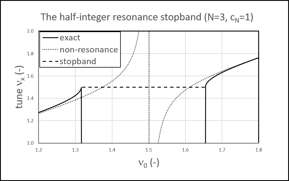
Figure 17: Illustration of the half-integer resonance stopband

Appendix E Analytical summation of the series expansions

The summations in tune expressions given in Eqs. (48,63) can be done analytically and the coefficients $a_{N},b_{N},c_{N},d_{N}$ can be expressed in elementary mathematical functions. In order to achieve this, all rational fractions of polynomials (with respect to $k$ since $n=(2k+1)N$) in the right hand sides of the equations have to be decomposed in a sum of simple rational fractions (see partial fraction decomposition[7, 8]). For example if we write the coefficient $\tilde{b}_{N}$ for the radial tune as:

$$\tilde{b}_{N}=\sum_{k=0}^{\infty}F(k)\ ,$$ (E1)

then we must decompose the function $F(k)$ as follow:

$$F(k)=\sum_{j=1}^{m}\frac{a_{j}}{(k+b_{j})^{p_{j}}}\ .$$ (E2)

Here $p_{j}=1,2,\dots$ is the power of the linear polynomial in the denominater of the fraction. Such a decomposition can be made for all the rational fractions that are present in Eqs. (48,63) and they have been derived in appendix F. For the form as given by $F(k)$, the summation can be carried out analytically and the result is [9, 10]:

$$\sum_{k=0}^{\infty}F(k)=\sum_{k=0}^{\infty}\sum_{j=1}^{m}\frac{a_{j}}{(k+b_{j})^{p_{j}}}=\sum_{j=1}^{m}\frac{(-1)^{p_{j}}}{(p_{j}-1)!}a_{j}\psi^{(p_{j}-1)}(b_{j})\ .$$ (E3)

Here $\psi^{(n})$ is the polygamma function [11, 12] of order $n$. The variables $b_{j}$ may be imaginary or complex. In order the series to converge, it is required that the sum of coefficients $a_{j}$ that correspond to linear powers $p_{j}=1$ must be equal zero.

$$\sum_{j\rightarrow p_{j}=1}^{m}a_{j}=0\ .$$ (E4)

This requirement is met for all the rational fractions that are present in Eqs. (48,63). We note that the reflection relation for the polygamma function[11, 12] must be used in order to express the final results in elementary mathematical functions. We show as an example the derivation for the coefficient $\tilde{b}_{N}$ in Eqs. (48). For convenience we define $n=mN=(2k+1)N$ and $\alpha=\sqrt{1+\bar{\mu}^{\prime}}/N$. We write for $\tilde{b}_{N}$

$$\tilde{b}_{N} =\frac{3(1+\bar{\mu}^{\prime})}{N^{4}}\sum_{k=0}^{\infty}\frac{1}{(m^{2}-4\alpha^{2})(m^{2}-\alpha^{2})}\ ,$$

$$=\frac{3\alpha^{2}}{N^{2}}\sum_{k=0}^{\infty}\left(\frac{1}{m^{2}-4\alpha^{2}}-\frac{1}{m^{2}-\alpha^{2}}\right)\ ,$$

$$=\frac{3\alpha}{4N^{2}}\sum_{k=0}^{\infty}\left(\frac{1}{m-2\alpha}-\frac{1}{m+2\alpha}-2{{(}}\frac{1}{m-\alpha}-\frac{1}{m+\alpha}{{)}}\right)\ ,$$

$$=\frac{3\alpha}{8N^{2}}\sum_{k=0}^{\infty}\left(\frac{1}{k+\frac{1-2\alpha}{2}}-\frac{1}{k+\frac{1+2\alpha}{2}}-2{{(}}\frac{1}{k+\frac{1-\alpha}{2}}-\frac{1}{k+\frac{1+\alpha}{2}}{{)}}\right)\ ,$$

$$=\frac{3\alpha}{8N^{2}}\left(-\psi(\frac{1-2\alpha}{2})+\psi(\frac{1+2\alpha}{2})-2{{(}}-\psi(\frac{1-\alpha}{2})+\psi(\frac{1+\alpha}{2}){{)}}\right)\ ,$$

$$=\frac{3\alpha}{8N^{2}}\left(-\psi(1-\frac{1+2\alpha}{2})+\psi(\frac{1+2\alpha}{2})-2{{(}}-\psi(1-\frac{1+\alpha}{2})+\psi(\frac{1+\alpha}{2}){{)}}\right)\ ,$$

$$=\frac{3\alpha}{8N^{2}}\left(-\pi\frac{\cos(\frac{1+2\alpha}{2})\pi}{\sin(\frac{1+2\alpha}{2})\pi}+2\pi\frac{\cos(\frac{1+\alpha}{2})\pi}{\sin(\frac{1+\alpha}{2})\pi}\right)\ .$$

$$=\frac{3\alpha\pi}{8N^{2}}\left(\tan(\pi\alpha)-2\tan(\pi\alpha/2)\right)\ .$$

Here $\psi$ is the digamma function (the polygamma function of order zero). In the last step we used the reflection relation for the polygamma function. For the digamma function this relation is:

$$\psi(1-z)-\psi(z)=\pi\cot\pi z\ .$$

An analogue but more general reflection relation exist (and has been used in our derivations) for the polygamma function. The same method as illustrated here has been applied for all series summations in our derivations (for the radial and vertical tunes and also for the stopband limits of the half-integer resonance). For the stopband limits we also needed to use the recurrance relation of the polygamma function. For the digamma function this relation takes the following form:

$$\psi(1+z)=\psi(z)+\frac{1}{z}\ .$$

Appendix F Partial fraction decomposition

We show details of the partial fraction decomposition as needed for the explicit evaluation of the series summations in the expression for the radial tune (Eq. (48)), the vertical tune (Eq. (63)) and the stopband limits of the half-integer resonance (Eqs. (81)) . In these series summations we first replace $n^{2}$ by $n^{2}=N^{2}m^{2}$ and define $\alpha^{2}=(1+\bar{\mu}^{\prime})/N^{2}$ and $\beta^{2}=4(1+\bar{\mu}^{\prime})/N^{2}$ (for the radial tune) and $\beta^{2}=-4\bar{\mu}^{\prime}/N^{2}$ (for the vertical tune). The decomposition is done in two steps. In the first (preliminary) step, the parameter $p$ is inserted for $m^{2}$ and $\alpha^{2}$ and $\beta^{2}$ are replaced by $\tilde{\alpha}$ and $\tilde{\beta}$ respectively. The following decompositions are obtained in the first step:

$$\frac{1}{p(p-\bar{\alpha})}=\frac{1}{\bar{\alpha}}(\frac{1}{p-\bar{\alpha}}-\frac{1}{p})$$

$$\frac{p}{(p-\bar{\alpha})^{2}(p-\bar{\beta})}=\frac{1}{(\bar{\alpha}-\bar{\beta})^{2}}{{(}}\frac{\bar{\beta}}{p-\bar{\beta}}-\frac{\bar{\beta}}{p-\bar{\alpha}}+\frac{\bar{\alpha}(\bar{\alpha}-\bar{\beta})}{(p-\bar{\alpha})^{2}}{{)}}\ ,$$

$$\frac{1}{(p-\bar{\alpha})^{2}(p-\bar{\beta})}=\frac{1}{(\bar{\alpha}-\bar{\beta})^{2}}{{(}}\frac{1}{p-\bar{\beta}}-\frac{1}{p-\bar{\alpha}}+\frac{\bar{\alpha}-\bar{\beta}}{(p-\bar{\alpha})^{2}}{{)}}\ ,$$

$$\frac{1}{p(p-\bar{\alpha})^{2}(p-\bar{\beta})}=\frac{1}{\bar{\alpha}^{2}\bar{\beta}(\bar{\alpha}-\bar{\beta})^{2}}{{(}}-\frac{(\bar{\alpha}-\bar{\beta})^{2}}{p}+\frac{\bar{\alpha}^{2}}{p-\bar{\beta}}+\frac{(\bar{\alpha}-\bar{\beta})^{2}-\bar{\alpha}^{2}}{p-\bar{\alpha}}+\frac{\bar{\alpha}\bar{\beta}(\bar{\alpha}-\bar{\beta})}{(p-\bar{\alpha})^{2}}{{)}}\ ,$$

$$\frac{p}{(p-\bar{\alpha})^{2}}=\frac{1}{p-\bar{\alpha}}+\frac{\bar{\alpha}}{(p-\bar{\alpha})^{2}}\ ,$$

$$\frac{1}{p(p-\bar{\alpha})^{2}}=\frac{1}{\bar{\alpha}^{2}}{{(}}\frac{1}{p}-\frac{1}{p-\bar{\alpha}}+\frac{\bar{\alpha}}{(p-\bar{\alpha})^{2}}{{)}}\ ,$$

$$\frac{1}{p(p-\bar{\alpha})^{3}}=\frac{1}{\bar{\alpha}^{3}}{{(}}-\frac{1}{p}+\frac{1}{p-\bar{\alpha}}-\frac{\bar{\alpha}}{(p-\bar{\alpha})^{2}}+\frac{\bar{\alpha}^{2}}{(p-\bar{\alpha})^{3}}{{)}}\ ,$$

$$\frac{p}{(p-\bar{\alpha})}=-\frac{1}{\bar{\alpha}}{{(}}\frac{1}{p}-\frac{1}{(p-\bar{\alpha})}{{)}}\ ,$$

$$\frac{p}{(p-\bar{\alpha})^{2}}=\frac{1}{(p-\bar{\alpha})}+\frac{\bar{\alpha}}{(p-\bar{\alpha})^{2}}\ ,$$

$$\frac{p}{(p-\bar{\alpha})^{3}}=\frac{1}{(p-\bar{\alpha})^{2}}+\frac{\bar{\alpha}}{(p-\bar{\alpha})^{3}}\ ,$$

$$\frac{1}{(p-\bar{\alpha})^{3}}=\mbox{already fully decomposed form}\ ,$$

$$\frac{1}{(p-\bar{\alpha})(p-\bar{\beta})}=\frac{1}{\bar{\alpha}-\bar{\beta}}{{(}}\frac{1}{(p-\bar{\alpha})}-\frac{1}{(p-\bar{\beta})}{{)}}\ .$$

In the second step each of the terms in the right hand sides of above expressions are further decomposed by inserting for $p,\tilde{\alpha},\tilde{\beta}$ the original parameters $m^{2},\alpha^{2},\beta^{2}$ respectively. We obtain the final expressions below for the radial tune and the vertical tune. Note that some of the decompositions for the radial tune also are used for the vertical tune. In the right hand sides of the final expressions we have to substitute $m=2k+1$, as $k$ is the summation index to be used in the series summations.

F.1 Radial tune decompositions

$$\frac{1}{m^{2}(m^{2}-\alpha^{2})}=\frac{1}{2\alpha^{3}}{{(}}(\frac{1}{m-\alpha}-\frac{1}{m+\alpha})-\frac{2\alpha}{m^{2}}{{)}}\ ,$$

$$\frac{1}{(m^{2}-\alpha^{2})^{2}}=\frac{1}{4\alpha^{3}}{{(}}-(\frac{1}{m-\alpha}-\frac{1}{m+\alpha})+\alpha(\frac{1}{(m-\alpha)^{2}}+\frac{1}{(m+\alpha)^{2}}){{)}}\ ,$$

$$\frac{1}{m^{2}(m^{2}-\alpha^{2})^{2}}=\frac{1}{4\alpha^{5}}{{(}}\frac{4\alpha}{m^{2}}-3(\frac{1}{m-\alpha}-\frac{1}{m+\alpha})+\alpha(\frac{1}{(m-\alpha)^{2}}+\frac{1}{(m+\alpha)^{2}}){{)}}\ ,$$

$$\frac{1}{m^{2}-\alpha^{2}}=\frac{1}{2\alpha}{{(}}\frac{1}{m-\alpha}-\frac{1}{m+\alpha}{{)}}\ ,$$

$$\frac{1}{m^{2}-4\alpha^{2}}=\frac{1}{4\alpha}{{(}}\frac{1}{m-2\alpha}-\frac{1}{m+2\alpha}{{)}}\ ,$$

$$\frac{1}{(m^{2}-\alpha^{2})(m^{2}-4\alpha^{2})}=\frac{1}{12\alpha^{3}}{{(}}(\frac{1}{m-2\alpha}-\frac{1}{m+2\alpha})-2(\frac{1}{m-\alpha}-\frac{1}{m+\alpha}){{)}}\ ,$$

$$\frac{1}{m^{2}(m^{2}-\alpha^{2})(m^{2}-4\alpha^{2})}=\frac{1}{48\alpha^{5}}{{(}}\frac{12\alpha}{m^{2}}+(\frac{1}{m-2\alpha}-\frac{1}{m+2\alpha})-8(\frac{1}{m-\alpha}-\frac{1}{m+\alpha}){{)}}\ ,$$

$$\frac{m^{2}}{(m^{2}-\alpha^{2})^{2}(m^{2}-4\alpha^{2})}=\frac{1}{36\alpha^{3}}{{(}}4(\frac{1}{m-2\alpha}-\frac{1}{m+2\alpha})-5(\frac{1}{m-\alpha}-\frac{1}{m+\alpha})$$

$$\hskip 142.26378pt-3\alpha(\frac{1}{(m-\alpha)^{2}}+\frac{1}{(m+\alpha)^{2}}){{)}}\ ,$$

$$\frac{1}{(m^{2}-\alpha^{2})^{2}(m^{2}-4\alpha^{2})}=\frac{1}{36\alpha^{5}}{{(}}(\frac{1}{m-2\alpha}-\frac{1}{m+2\alpha})+(\frac{1}{m-\alpha}-\frac{1}{m+\alpha})$$

$$\hskip 142.26378pt-3\alpha(\frac{1}{(m-\alpha)^{2}}+\frac{1}{(m+\alpha)^{2}}){{)}}\ ,$$

$$\frac{1}{m^{2}(m^{2}-\alpha^{2})^{2}(m^{2}-4\alpha^{2})}=\frac{1}{36\alpha^{7}}{{(}}\frac{1}{4}(\frac{1}{m-2\alpha}-\frac{1}{m+2\alpha})+7(\frac{1}{m-\alpha}-\frac{1}{m+\alpha})$$

$$\hskip 142.26378pt-\frac{9\alpha}{m^{2}}-3\alpha(\frac{1}{(m-\alpha)^{2}}+\frac{1}{(m+\alpha)^{2}}){{)}}\ ,$$

$$\frac{1}{m^{2}(m^{2}-\alpha^{2})^{3}}=\frac{1}{16\alpha^{7}}{{(}}15(\frac{1}{m-\alpha}-\frac{1}{m+\alpha})-\frac{16\alpha}{m^{2}}-7\alpha(\frac{1}{(m-\alpha)^{2}}+\frac{1}{(m+\alpha)^{2}})$$

$$\hskip 142.26378pt+2\alpha^{2}(\frac{1}{(m-\alpha)^{3}}-\frac{1}{(m+\alpha)^{3}}){{)}}\ .$$

F.2 Vertical tune decompositions

$$\frac{m^{2}}{(m^{2}-\alpha^{2})^{3}}=\frac{1}{16\alpha^{3}}{{(}}-(\frac{1}{m-\alpha}-\frac{1}{m+\alpha})+\alpha(\frac{1}{(m-\alpha)^{2}}+\frac{1}{(m+\alpha)^{2}})$$

$$\hskip 142.26378pt+2\alpha^{2}(\frac{1}{(m-\alpha)^{3}}-\frac{1}{(m+\alpha)^{3}}){{)}}\ ,$$

$$\frac{1}{(m^{2}-\alpha^{2})^{3}}=\frac{3}{16\alpha^{5}}{{(}}(\frac{1}{m-\alpha}-\frac{1}{m+\alpha})-\alpha(\frac{1}{(m-\alpha)^{2}}+\frac{1}{(m+\alpha)^{2}})$$

$$\hskip 142.26378pt+\frac{2\alpha^{2}}{3}(\frac{1}{(m-\alpha)^{3}}-\frac{1}{(m+\alpha)^{3}}){{)}}\ ,$$

$$\frac{m^{2}}{(m^{2}-\alpha^{2})^{2}(m^{2}-\beta^{2})}=\frac{1}{4(\alpha^{2}-\beta^{2})^{2}}{{(}}2\beta(\frac{1}{m-\beta}-\frac{1}{m+\beta})$$

$$\hskip 56.9055pt-\frac{\alpha^{2}+\beta^{2}}{\alpha}(\frac{1}{m-\alpha}-\frac{1}{m+\alpha})+(\alpha^{2}-\beta^{2})(\frac{1}{(m-\alpha)^{2}}+\frac{1}{(m+\alpha)^{2}}){{)}}\ ,$$

$$\frac{1}{(m^{2}-\alpha^{2})^{2}(m^{2}-\beta^{2})}=\frac{1}{4(\alpha^{2}-\beta^{2})^{2}}{{(}}\frac{2}{\beta}(\frac{1}{m-\beta}-\frac{1}{m+\beta})$$

$$\hskip 56.9055pt-(\frac{3\alpha^{2}-\beta^{2}}{\alpha^{3}})(\frac{1}{m-\alpha}-\frac{1}{m+\alpha})+(\frac{\alpha^{2}-\beta^{2}}{\alpha^{2}})(\frac{1}{(m-\alpha)^{2}}+\frac{1}{(m+\alpha)^{2}}){{)}}\ ,$$

$$\frac{1}{m^{2}(m^{2}-\alpha^{2})^{2}(m^{2}-\beta^{2})}=\frac{1}{2\beta^{3}(\alpha^{2}-\beta^{2})^{2}}(\frac{1}{m-\beta}-\frac{1}{m+\beta})-\frac{1}{\alpha^{4}\beta^{2}}\frac{1}{m^{2}}$$

$$\hskip 28.45274pt+\frac{3\beta^{2}-5\alpha^{2}}{4\alpha^{5}(\alpha^{2}-\beta^{2})^{2}}(\frac{1}{m-\alpha}-\frac{1}{m+\alpha})+\frac{1}{4\alpha^{4}(\alpha^{2}-\beta^{2})}(\frac{1}{(m-\alpha)^{2}}+\frac{1}{(m+\alpha)^{2}})\ .$$

$$\frac{m^{2}}{(m^{2}-\alpha^{2})^{2}}=\frac{1}{4\alpha}(\frac{1}{m-\alpha}-\frac{1}{m+\alpha})+\frac{1}{4}(\frac{1}{(m-\alpha)^{2}}+\frac{1}{(m+\alpha)^{2}})\ ,$$

$$\frac{1}{(m^{2}-\alpha^{2})(m^{2}-\beta^{2})}=\frac{1}{(\alpha^{2}-\beta^{2})}{{(}}\frac{1}{2\alpha}(\frac{1}{m-\alpha}-\frac{1}{m+\alpha})-\frac{1}{2\beta}(\frac{1}{m-\beta}-\frac{1}{m+\beta}){{)}}\ ,$$

$$\frac{1}{m^{2}(m^{2}-\alpha^{2})(m^{2}-\beta^{2})}=\frac{1}{2(\alpha^{2}-\beta^{2})}{{(}}\frac{1}{\alpha^{3}}(\frac{1}{m-\alpha}-\frac{1}{m+\alpha})-\frac{1}{\beta^{3}}(\frac{1}{m-\beta}-\frac{1}{m+\beta}){{)}}$$

$$\hskip 113.81102pt+\frac{1}{\alpha^{2}\beta^{2}}\frac{1}{m^{2}}\ ,$$

$$\frac{1}{m^{2}(m^{2}-\alpha^{2})}=-\frac{1}{\alpha^{2}}{{(}}\frac{1}{m^{2}}-\frac{1}{2\alpha}(\frac{1}{m-\alpha}-\frac{1}{m+\alpha}){{)}}\ .$$

F.3 Summation of decomposed fractions

Once the partial fractions in the series expressions have been decomposed, each of the seperate basic contributions have to be analytically calculated. Here we use the method as explained in appendix E. With $\alpha^{2}=\gamma^{2}/N^{2}$ and $\beta^{2}=-4(\gamma^{2}-1)/N^{2}$ and taking into account that $\alpha^{2}>0$ and $\beta^{2}<0$, we obtain the following basic contributions:

$$\sum_{k=0}^{\infty}\frac{1}{m-\alpha}-\frac{1}{m+\alpha} =\frac{\pi}{2}\tan(\frac{\pi\gamma}{2N})\ ,$$

$$\sum_{k=0}^{\infty}\frac{1}{m-2\alpha}-\frac{1}{m+2\alpha} =\frac{\pi}{2}\tan(\frac{\pi\gamma}{N})\ ,$$

$$\sum_{k=0}^{\infty}\frac{1}{m-\beta}-\frac{1}{m+\beta} =\frac{i\pi}{2}\tanh(\frac{\pi\sqrt{\gamma^{2}-1}}{N})\ ,$$

$$\sum_{k=0}^{\infty}\frac{1}{m^{2}} =\frac{\pi^{2}}{8}\ ,$$

$$\sum_{k=0}^{\infty}\frac{1}{(m-\alpha)^{2}}+\frac{1}{(m+\alpha)^{2}} =\frac{\pi^{2}}{4}\left(1+\tan^{2}(\frac{\pi\gamma}{2N})\right)\ ,$$

$$\sum_{k=0}^{\infty}\frac{1}{(m-\alpha)^{3}}-\frac{1}{(m+\alpha)^{3}} =\frac{\pi^{3}}{8}\tan(\frac{\pi\gamma}{2N})\left(1+\tan^{2}(\frac{\pi\gamma}{2N})\right)\ ,$$

$$\sum_{k=1}^{\infty}\frac{1}{m-\tfrac{1}{2}}-\frac{1}{m+\tfrac{1}{2}} =\frac{\pi}{2}-\frac{4}{3}\ ,$$

$$\sum_{k=1}^{\infty}\frac{1}{m-1}-\frac{1}{m+1} =\frac{1}{2}\ ,$$

$$\sum_{k=1}^{\infty}\frac{1}{(m-\tfrac{1}{2})^{2}}-\frac{1}{(m+\tfrac{1}{2})^{2}} =\frac{\pi^{2}}{2}-\frac{40}{9}\ ,$$

$$\sum_{k=1}^{\infty}\frac{1}{m^{2}} =\frac{\pi^{2}}{8}-1\ .$$

where $i$ is the imaginairy unit and where $m=2k+1$ must be substituted.

Appendix G Some properties of canonical systems

G.1 The Hamiltonian

Suppose an orbit $x(\theta)$ has to be calculated from the two differential equations:

$$p^{\prime} = \frac{dp}{d\theta}\ =\ f(p,x,\theta)\ ,$$ (G1)

$$x^{\prime} = \frac{dx}{d\theta}\ =\ g(p,x,\theta)\ ,$$ (G2)

and that $f$ and $g$ obey the relation:

$$\frac{\partial f}{\partial p}+\frac{\partial g}{\partial x}=0\ .$$

We can define a function $H(p,x,\theta)$, by:

$$f=-\frac{\partial H}{\partial x}\ ,\ \ \ g=\frac{\partial H}{\partial p}\ ,$$

so that Eqs. (G1-G2) become:

$$\frac{dp}{d\theta} = -\frac{\partial H}{\partial x}\ ,$$ (G3)

$$\frac{dx}{d\theta} = +\frac{\partial H}{\partial p}\ .$$ (G4)

The variables $p$ and $x$ are called canonical variables and the function $H$ is called the Hamiltonian. This canonical system has the property that an area occupied by a group of points in the $p,x$-plane (called the phase space) remains constant during the motion. This is the Liouville theorem. From Eqs. (G3-G4) one finds that the total derivative of $H$ with respect to $\theta$ is equal to its partial derivative:

$$\frac{dH}{d\theta}=\frac{\partial H}{\partial\theta}\ .$$

This means that $H$ is constant of motion if $H$ does not contain the independent variable $\theta$ explicitly. In this case one gets a very useful semi quantative picture of the motion in the $p,x$-plane , representing the real motion $x(\theta)$ by observing that the points move on the contours $H$ = constant. An extremum of $H$ gives a stable stationary position $p$ = constant, $x$ = constant (a stable fixed point). A sadle point in the $H$ surface gives a metastable position (unstable fixed point).

G.2 Canonical transformations

An important property of a canonical system is the possibility to make a transformation from the existing variables $p,x$ to new variables $P,X$:

$$P = P(p,x,\theta)\ ,$$

$$X = X(p,x,\theta)\ ,$$

such that $P$ and $X$ can be derived from a new Hamiltonian $K$ similar to Eqs. (G3,G4):

$$\frac{dP}{d\theta} = -\frac{\partial K}{\partial X}\ ,$$ (G5)

$$\frac{dX}{d\theta} = +\frac{\partial K}{\partial P}\ .$$ (G6)

A necessary and sufficient condition is that the ratio $R$ of the area of a region in the $p,x$ plane to the area of the corresponding region in the $P,X$ plane is independent of $p,x$ and $\theta$. This means that the determinant of the Jacobian matrix of the transformation must be constant:

$$R=\begin{vmatrix}\partial P/\partial p&\partial P/\partial x\\ \partial X/\partial p&\partial X/\partial x\end{vmatrix}=\mbox{constant}\ .$$ (G7)

The new Hamiltonian $K$ is obtained from the orginal $H$ as follows:

$$K=R*H+\Xi(P,X,\theta)\ ,$$ (G8)

where the function $\Xi$ is obtained from:

$$\frac{\partial\Xi}{\partial P} = +\frac{\partial X}{\partial\theta}\ ,$$

$$\frac{\partial\Xi}{\partial X} = -\frac{\partial P}{\partial\theta}\ .$$

Canonical transformations with $R=1$ can be obtained from so called generating functions[13]. Denote the original variables as $(x,p)$, the new variables as $(X,P)$ and the independent variable as $\theta$.

The first type of generating function $G_{1}$ depends on the original coordinate $x$ and the new coordinate $X$. The transformation is defined by:

$$p=\frac{\partial G_{1}}{\partial x}\ ,\ \ \ P=-\frac{\partial G_{1}}{\partial X}\ .$$ (G9)

The second type $G_{2}$ depends on the original coordinate $x$ and the new momentum $P$. The transformation is defined by:

$$p=\frac{\partial G_{2}}{\partial x}\ ,\ \ \ X=\frac{\partial G_{2}}{\partial P}\ .$$ (G10)

The third type $G_{3}$ depends on the original momentum $p$ and the new coordinate $X$. The transformation is defined by:

$$x=-\frac{\partial G_{3}}{\partial p}\ ,\ \ \ P=-\frac{\partial G_{3}}{\partial X}\ .$$ (G11)

The fourth type $G_{4}$ depends on the original momentum $p$ and the new momentum $P$. The transformation is defined by:

$$x=-\frac{\partial G_{4}}{\partial p}\ ,\ \ \ X=\frac{\partial G_{4}}{\partial P}\ .$$ (G12)

In all four cases, the new Hamiltonian $K$ is obtained as:

$$K=H+\frac{\partial G}{\partial\theta}\ .$$

G.3 Orbits in the neighborhood of a known solution

Let us assume that we have a particular solution $p_{e}(\theta),x_{e}(\theta)$ for a given Hamiltonian $H(p,x,\theta)$. In this case $p_{e}$ and $x_{e}$ obey the equations similar to Eq. (G3,G4):

$$\frac{dp_{e}}{d\theta} = -\frac{\partial H}{\partial x_{e}}\ ,$$ (G13)

$$\frac{dx_{e}}{d\theta} = +\frac{\partial H}{\partial p_{e}}\ .$$ (G14)

We want to study the motion in the neighborhood of $p_{e},x_{e}$ and therefore introduce the new variables $P,X$ as:

$$P=p-p_{e}(\theta)\ ,$$

$$X=x-x_{e}(\theta)\ .$$

This transformation can be obtained from the type 2 generating function (see Eqs. (G10)):

$$G = G_{2}(P,x)=xP-x_{e}P+p_{e}x\ ,$$

$$X = \frac{\partial G_{2}}{\partial P}=x-x_{e}\ ,$$

$$p = \frac{\partial G_{2}}{\partial x}=P+p_{e}\ ,$$

$$\frac{\partial G}{\partial\theta} = -\dot{x}_{e}P+\dot{p}_{e}(X+x_{e})\ .$$

We now expand the Hamiltonian $H$ around the solution $p_{e},x_{e}$ as follows:

$$H=P\frac{\partial H}{\partial p_{e}}+X\frac{\partial H}{\partial x_{e}}+\frac{1}{2}P^{2}\frac{\partial^{2}H}{\partial p_{e}^{2}}+\dots\ .$$

Note that the zero-degree term in this expansion does not contribute to the form of the equations of motion and therefore can be omitted. The new Hamiltion is obtained as $K=H+\partial G/\partial\theta$ giving:

$$K(P,X,\theta)=P\frac{\partial H}{\partial p_{e}}+X\frac{\partial H}{\partial x_{e}}+\frac{1}{2}P^{2}\frac{\partial^{2}H}{\partial p_{e}^{2}}+\dots-\dot{x}_{e}P+\dot{p}_{e}X\ .$$

But by virtue of Eqs. (G13,G14), the first degree terms in the above expression for $K$ cancel each other. So, when studying the motion in the neighborhood of a known solution we can in the expansion of the new Hamiltonian, ignore the first degree terms in $P,X$ and only take into account the quadratic degree terms and the higher degree terms:

$$K(P,X,\theta)=\frac{1}{2}P^{2}\frac{\partial^{2}H}{\partial p_{e}^{2}}+PX\frac{\partial^{2}H}{\partial p_{e}\partial x_{e}}+\frac{1}{2}X^{2}\frac{\partial^{2}H}{\partial x_{e}^{2}}+\frac{1}{6}P^{3}\frac{\partial^{3}H}{\partial p_{e}^{3}}+\dots\ .$$

The quadratic terms correspond to the linear approximation of the motion with respect to the known solution. The higher degree terms must be included when studying nonlinear effects.

G.4 The normal form of a quadratic Hamiltonian

Consider a quadratic Hamiltonian of the following form:

$$H(\pi,\xi,\theta)=\tfrac{1}{2}f\pi^{2}+g\pi\xi+\tfrac{1}{2}h\xi^{2}\ .$$

where $f,g$ and $h$ are functions of $\theta$ only and where $f\neq 0$. We want to reduce this Hamiltonian to its normal form defined as:

$$K(P,X,\theta)=\tfrac{1}{2}P^{2}+\tfrac{1}{2}Q(\theta)X^{2}\ .$$ (G15)

We first eliminate the coefficient $f$ in the term with $\pi^{2}$, using the following type 3 generating function:

$$G = G_{3}(\pi,\bar{\xi},\theta)=-\pi\bar{\xi}f^{\tfrac{1}{2}}\ ,$$

$$\bar{\pi} = \pi f^{\tfrac{1}{2}}\ ,$$

$$\bar{\xi} = \xi f^{-\tfrac{1}{2}}\ ,$$

$$\partial G/\partial\theta = -\tfrac{1}{2}f^{-1}\dot{f}\bar{\pi}\bar{\xi}\ .$$

This gives for the new Hamiltonian:

$$\bar{H}(\bar{\pi},\bar{\xi},\theta)=\tfrac{1}{2}\bar{\pi}^{2}+(g-\tfrac{1}{2}f^{-1}\dot{f})\bar{\pi}\bar{\xi}+\tfrac{1}{2}fh\ \bar{\xi}^{2}\ .$$

With a second transformation (from $\bar{\pi},\bar{\xi}$ to $P,X$) we want to remove the term $\bar{\pi}\bar{\xi}$ in $\bar{H}$. When in the final Hamiltonian $K$, such a cross-term is not present, we will have $\dot{X}=\partial K/\partial P=P$. From this we can deduce the transformation that will be needed by taking $X=\bar{\xi}$ giving

$$X=\bar{\xi}\ ,\hskip 56.9055ptP=\dot{X}=\dot{\bar{\xi}}\ ,$$

and where we get $\dot{\bar{\xi}}$ from $\partial\bar{H}/\partial\bar{\pi}$. This leads us to the following transformation:

$$P = \bar{\pi}\leavevmode\nobreak\ (g-\tfrac{1}{2}f^{-1}\dot{f})\bar{\xi}\ ,$$

$$X = \bar{\xi}\ .$$

$$G = G_{3}(\bar{\pi},X,\theta)=-\bar{\pi}X-(g-\tfrac{1}{2}f^{-1}\dot{f})X^{2}/2\ .$$

With this the new Hamiltonian $K$ as given in Eq. (G15) is obtained and the function $Q$ is given by:

$$Q(\theta)=fh-(g-\tfrac{1}{2}f^{-1}\dot{f})^{2}-\frac{d}{d\theta}(g-\tfrac{1}{2}f^{-1}\dot{f})\ .$$

The full transformation (and its inverse) is given by:

$$P = f^{\tfrac{1}{2}}\pi+(g-\tfrac{1}{2}f^{-1}\dot{f})f^{-\tfrac{1}{2}}\xi\ ,\hskip 56.9055ptX=f^{-\tfrac{1}{2}}\xi\ ,$$

$$\pi = f^{-\tfrac{1}{2}}\left[P-(g-\tfrac{1}{2}f^{-1}\dot{f})X\right]\ ,\hskip 51.21504pt\xi=f^{\tfrac{1}{2}}X\ .$$

References

- [1] M. M. Gordon, “Orbit Properties of the Isochronous Cyclotron Ring with Radial Sectors”, in Anals of Physics, vol. 50, pp. 571-597, 1968.
- [2] V. I. Danilov, Yu. N. Denisov, V. P. Dmitrievskij, V. P. Dzhelepov, A. A. Glazov et al., “Cyclotron With Space Variation Of The Magnetic Field”, in Proc. 2nd Int. Conf. High-Energy Accelerators and Instrumentation, HEACC 1959, CERN, Geneva, Switzerland, September 14-19, 1959, pp. 211-226.
- [3] H. L. Hagedoorn and N. F. Verster, “Orbits in an AVF Cyclotron”, in Nuclear Instruments and Methods, vol. 18,19, pp. 201-228, 1962 .
- [4] Y. Jongen, W. Kleeven and S. Zaremba, “New Cyclotron Developments at IBA”, in Proc. 17th Int. Conf. Cyclotrons and their Applications, Tokyo, Japan, 2004, pp. 110-114.
- [5] Y. Jongen et al., “IBA C400 Cyclotron Project for Hadron Therapy”, in Proc. 18th Int. Conf. Cyclotrons and their Applications, Giardini Naxos, Italy, 2000, pp. 151-153.
- [6] Y. Jongen et al., “IBA-JINR 400 MeV/u Superconducting Cyclotron for Hadron Therapy”, in Proc. 19th Int. Conf. Cyclotrons and their Applications, Lanzhou, China, 2010, pp. 404-409.
- [7] Partial fraction decomposition https://en.wikipedia.org/wiki/Partial_fraction_decomposition.
- [8] Ron Larson, “Algebra & Trigonometry”, Cengage Learning, 2016, ISBN 9781337271172.
- [9] Digamma function, https://en.wikipedia.org/wiki/Digamma_function#Computation_and_approximation.
- [10] M. Abramowitz, and I. A. Stegun, eds., “Handbook of Mathematical Functions with Formulas, Graphs, and Mathematical Tables”, 9th ed., “6.3 psi (Digamma) Function”, Dover Publications, New York, p. 258–259, 1970.
- [11] Polygamma function, https://en.wikipedia.org/wiki/Polygamma_function.
- [12] M. Abramowitz, and I. A. Stegun, eds., “Handbook of Mathematical Functions with Formulas, Graphs, and Mathematical Tables”,9th ed., “6.4 Polygamma Functions”, Dover Publications, New York, pp. 260, 1970.
- [13] Herbert Goldstein, “Classical Mechanics”, 2nd ed., Addison-Wesley Publishing Company, 1980, ISBN 0-201-02918-9.