Partially coherent Airy beams: A cross-spectral density approach

Abstract

Airy beams are known for displaying shape invariance and self-acceleration along the transverse direction while they propagate forwards. Although these properties could be associated with the beam coherence, it has been revealed that they also manifest in the case of partially coherent Airy-type beams. Here, these properties are further investigated by introducing and analyzing a class of partially coherent Airy beams under both infinite and finite energy conditions. The key element within the present approach is the so-called cross-spectral density, which enables a direct connection with the quantum density matrix, making the analysis exportable to the quantum realm to study the dynamics of Airy wave packets acted by both incoherence and decoherence. As it is shown, in the case of infinite energy beams both properties are preserved even under the circumstance of total incoherence provided the underlying structure of the beam remains equal to that of an Airy beam. In the case of finite energy beams, a situation closer to a realistic scenario, as experimental beams cannot have an infinite extension, it is shown that a propagation range along which both properties are preserved can be warranted. This is controlled by a critical distance, which depends on the spread range determined by the parameters ruling the extension of random field spatial fluctuations. Such a distance is determined by defining a position-dependent parameter that quantifies the degree of overlapping between the propagated beam and the input one displaced by an amount equivalent to the propagation distance.

I Introduction

Airy wave packets are known for exhibiting two intriguing and counter intuitive properties: when they are freely released in space, their propagation is dispersionless and uniformly accelerated. This self-accelerating solution to the free-particle nonrelativistic Schrödinger equation was first noticed by Berry and Balazs in the late 1970s [1], who provided a semiclassical explanation to this behavior based on the concept of caustic. Yet, by invoking the equivalence principle, it is also possible an alternative explanation, as it was suggested shortly afterwards by Greenberger [2]. Accordingly, the Airy wave packet can be understood as the stationary solution for a free-falling system in a uniform gravitational field. Later works have been aimed at finding first-principles derivations of these puzzling solutions [3], generalizing the behavior to higher dimensions [4], or even exploring ways to redirect electron Airy beams without causing any dispersion by means of magnetic fields [5].

Matter-wave Airy-type beams and their dynamics have also received attention in the context of nonlinear extensions of the Schrödinger equation. This is the case, for instance, of the Gross-Pitaevskii equation, a nonlinear Schrödinger equation accounting for the dynamics of Bose-Einstein condensates (BECs) in the mean-field (Hartree-Fock) approximation [6]. Within this context, it has been shown that, by properly controlling the amplitude and phase of the BEC, it is possible to make it to behave as an ordinary self-accelerating Airy beam, and also to produce an abrupt autofocusing [7]. Airy-type solutions for BECs confined within time-dependent harmonic traps have also been determined [8], which are shown to spontaneously break the parity and time-reversal symmetries. On the other hand, within the classical realm, experiments reported in the literature show the emergence of Airy-type solutions in surface gravity water waves [9, 10], where the behavior of such waves is ruled by equations isomorphic to Schrödinger’s one in the linear regime.

In spite of all the literature generated around Airy (matter-)wave packets at, say, a fundamental level, covering a wide variety of formal aspects and physical situations, it is worth noting how experimentally-oriented works involving matter waves are rather scarce instead. The first experimental realization and observation of free-electron Airy wave packets were reported by Voloch-Bloch et al. [11]. These Airy wave packets were produced by diffracting electron beams with nanoscale holograms. However, unlike Berry and Balazs formerly suggested, the beams generated were not direct solutions of the nonrelativistic Schrödinger equation, but paraxial solutions to the Klein-Gordon equation, which suffices to describe the slowly changing transverse electron motion in transmission electron microscopy. Interestingly, these works can be considered to be within the subject of electron beam shaping [12], aimed at producing nanostructured electron beams [13], which is in direct analogy to field of structured light beams, where paraxial treatments are also common.

Now, it is precisely within the above-mentioned scenario of paraxiality and structured light, where optical Airy beams have received much attention from an experimental point of view since the mid-2000s [14]. Note that translating the concept of Airy wave packet to the optical realm is straightforward by virtue of the well-known isomorphism exhibited by the nonrelativistic Schrödinger equation and the Helmholtz equation in paraxial form, with the longitudinal coordinate in the latter playing the role of the time in the former. By producing the appropriate hologram phase mask, Siviloglou et al. [15] reported on the first experimental evidence of light Airy beams (and of Airy beams, in general, since matter-wave realizations came several years later). In contrast to other types of structured light, Airy beams are characterized for keeping their shape invariance (a transverse profile with the form of an Airy function) while they propagate forward along the longitudinal coordinate, i.e., when they are observed at different output planes. Moreover, the transverse evolution of the beam manifests the self-accelerating motion of Airy wave packets, although this dependence is on the longitudinal coordinate (output plane position).

By definition, light Airy beams correspond to an ideal situation in which the beam has an infinite extension. Hence, they involve an unbound (infinite) amount of energy. To some extent, this behavior has been experimentally implemented and observed [15], but at the expense that, at some point (in space), the beam produced deviates from the ideal Airy beam behavior; obviously, it is not possible to implement a beam carrying an infinite amount of energy. In this regard, since the first experimental demonstrations of Airy beams, the interest has turned towards the so-called partially coherent Airy beams, which correspond to more realistic physical implementations of also shape-invariant self-accelerating light beams.

An appropriate tool to cope with the issue of partially coherent light is the cross-spectral density (CSD) [16]. As it is known, apart from Airy beams, a significant class of sources is characterized by keeping their shape invariant for paraxial propagation conditions at any distance from the source, except for a transverse scaling factor and a spherical curvature term. This invariance concerns the whole CSD of the field and hence both the profile displayed by the intensity distribution along the transverse direction and the coherence properties. When this condition is satisfied, the field CSD is said to be shape-invariant. Research on possible forms of CSDs giving rise to fields with peculiar propagation properties has been ongoing since the late 1970s (see, for instance, Ref. [17], and references therein). Yet, there is a major inconvenience in devising new CSD forms, as they are not generic two-point space functions. A necessary and sufficient condition for a function to represent a valid CSD is that it must be a non-negative definite Hermitian function [16]. Whenever this condition is satisfied, the CSD is said to be genuine or bona-fide; if the condition is not satisfied, then the function cannot represent the CSD of a possible physical source. In general, though, it is not easy to check the non-negativity of an integral kernel, although genuineness criteria have been introduced in the literature with this purpose [18, 19, 20, 21].

Here we approach and investigate partially coherent Airy-type beams from the point of view of their corresponding CSDs in cases of both finite and infinite energy. As it is shown, although the analysis in all cases starts from well-defined Airy functions, the introduction of random fluctuations and, more specifically, the spread functions that determine the spatial reach of such fluctuations are going to play a major role in the preservation of the beam properties, namely, shape-invariance and self-acceleration. In the infinite energy case, we show that these properties still remain even when the fast oscillations that characterize the decaying tail of Airy beams are smoothed out by the averaging over random realizations. This apparently counter intuitive behavior can be explained taking into account that a swarm of identical Airy beams still underneath the internal structure of the full beam, regardless of the extent of random fluctuations. Since all single Airy beams included in the random mixture are independent one another, their shape-invariance and self-acceleration properties remain unaffected, and hence also those of the resulting partially coherent beam. In the finite energy case, however, because additional constraints are set upon the random displacements (leading to correlations among them), both shape-invariance and self-acceleration can only be preserved up to a certain point. This validity range is a function of the parameters governing the spread of the random fluctuations, as it is shown by computing the overlapping between the propagated beam and the translated initial beam. Actually, by means of such calculations, it is shown that we can uniquely get an estimate of the range of output planes where the beams are still going to be behave in an Airy-type manner in simple terms.

According to the above discussion, the work is organized as follows. The main aspects involved in the CSD approach here considered and its application to the case of infinite energy are discussed in Sec. II. Without loss of generality, this is illustrated by considering a Gaussian spread function for the spatial random fluctuations acting on the beam at each position. In Sec. III, two types of finite-energy, partially coherent Airy beams are presented after generalizing the model of Sec. II with the introduction of spatial correlations between the random displacements. Although the starting point in the construction of each type of CSD is physically different, eventually the functional form displayed by the general expression is shown to be similar. Finally, the main conclusions extracted from the work are summarized in Sec. IV.

II Infinite Energy Beams

For simplicity, the analysis will be constrained to a single transverse direction instead of the full transverse plane, as we only need a transverse coordinate to investigate the Airy-beam properties of shape-invariance and self-acceleration in partially coherent beams. Thus, to start with, consider a field amplitude that satisfies the paraxial Helmholtz equation,

$$i\ \frac{\partial\mathcal{U}(x,z)}{\partial z}=-\frac{1}{2}\frac{\partial^{2}\mathcal{U}(x,z)}{\partial x^{2}},$$ (1)

where $x$ and $z$ denote, respectively, the transverse and longitudinal dimensionless coordinates (they are referred to a certain characteristic length $\ell$ and the wave number $k=2\pi/\lambda$, i.e., $x_{\rm dim}=\ell x$ and $z_{\rm dim}=k\ell^{2}z$). If a quasi-monochromatic beam consists of a number of random realizations of field amplitudes $\mathcal{U}$, all satisfying Eq. (1), it can be specified by its CSD,

$$\mathcal{W}(x,x^{\prime},z)=\langle\mathcal{U}^{*}(x,z)\ \!\mathcal{U}(x^{\prime},z)\rangle,$$ (2)

where the explicit dependence on the frequency is implicitly assumed.

The CSD (2) provides us with a map of two-point field correlations at a given output plane $z$, and hence with valuable information on the beam intensity distribution and coherence properties. Note that the beam intensity distribution is directly obtained from the diagonal of the CSD (i.e., for $x^{\prime}=x$) at a plane $z$, as

$$I(x,z)=\mathcal{W}(x,x,z),$$ (3)

while the off-diagonal elements render information about the coherence between two different points $x$ and $x^{\prime}$. Actually, there is a direct relationship between the CSD and quantifiers of the beam coherence properties, such as the complex degree of coherence [16],

$$\gamma(x,x^{\prime},z)=\frac{\mathcal{W}(x,x^{\prime},z)}{\sqrt{I(x,z)}\sqrt{I(x^{\prime},z)}}.$$ (4)

The modulus of this quantity ranges from 0, in the case of total incoherence, to a maximum smaller or equal to 1, in the case of full coherence. There are other related coherence quantifiers, such as the visibility [16] or the which-path distinguishability [22], which additionally allow us to establish a direct connection with matter waves, where the density operator plays the role of the CSD. In this regard, the discussion below can straightforwardly extended to the quantum realm.

Let us now consider that the field amplitude at the input plane $z=0$ is described by an Airy function,

$$Ai(x) = \frac{1}{\pi}\ \int_{0}^{\infty}\cos\left(\frac{u^{3}}{3}+xu\right)du$$ (5)

$$= \frac{1}{2\pi}\ \int_{-\infty}^{\infty}e^{i(u^{3}/3+xu)}du.$$

This function satisfies the orthogonality condition

$$\int_{-\infty}^{\infty}Ai(x-u)Ai(x-v)\ \!dx=\delta(u-v).$$ (6)

From the input ansatz, Eq. (5), we can obtain the field amplitude at any other output plane $z\neq 0$, solution of the paraxial Helmholtz equation, Eq. (1), by applying the free-space propagator. This propagated solution reads

$$Ai(x,z)=e^{i(x-z^{2}/6)z/2}Ai(x-z^{2}/4),$$ (7)

which is a complex-valued function, unlike $Ai(x)$. It can readily be seen that the amplitude of the field (7) is both shape invariant and self-accelerating, since

$$|Ai(x,z)|=|Ai(x-z^{2}/4)|,$$ (8)

i.e., the amplitude at the output plane $z$ is exactly the same as the amplitude resulting from moving the amplitude at $z=0$ from $x$ to $x-z^{2}/4$: Moreover, it is also seen that the whole field undergoes a net displacement that goes with the square of $z$, which, in analogy to Airy wave packets, is associated with an acceleration.

Consider now an arbitrary coherent superposition of Airy beams at the input plane $z=0$, where each of these beams is affected by a random displacement $\lambda$ and contributes to the superposition with an amplitude $c(\lambda)$. This combination produces a field amplitude

$$\bar{\mathcal{U}}(x,0)=\int c(\lambda)Ai(x-\lambda)\ \!d\lambda.$$ (9)

By virtue of the orthogonality relation (6), we have

$$c(\lambda)=\int\bar{\mathcal{U}}(x,0)Ai(x-\lambda)\ \!dx.$$ (10)

Because of the linearity of the superposition (9), at an arbitrary plane $z$, the field amplitude $\bar{\mathcal{U}}$ read as

$$\bar{\mathcal{U}}(x,z)=\int c(\lambda)Ai(x-\lambda,z)\ \!d\lambda.$$ (11)

Appealing to the identity (7), this field amplitude can be recast as

$$\bar{\mathcal{U}}(x,z)=\int c(\lambda)e^{i(x-\lambda-z^{2}/6)z/2}Ai(x-\lambda-z^{2}/4)\ \!d\lambda.$$ (12)

The field amplitude (12) describes a fully coherent beam with analogous properties to those displayed by the constituting Airy beams. Let us consider the case of a number of random realizations of $\bar{\mathcal{U}}(x,z)$. At $z=0$, the CSD describing this field reads as

$$\mathcal{W}(x,x^{\prime},0) = \langle\bar{\mathcal{U}}^{*}(x,0)\ \!\bar{\mathcal{U}}(x^{\prime},0)\rangle$$

$$= \iint\mathcal{C}_{0}(\lambda,\lambda^{\prime})Ai(x-\lambda)Ai(x^{\prime}-\lambda^{\prime})\ \!d\lambda d\lambda^{\prime},$$

where

$$\mathcal{C}_{0}(\lambda,\lambda^{\prime})\equiv\langle c^{*}(\lambda)c(\lambda^{\prime})\rangle$$ (14)

is a non-negative Hermitian function. This function provides us with information on possible correlations between two different displacements $\lambda$ and $\lambda^{\prime}$. Because (LABEL:eq9) has the functional form of a convolution integral, its spectrum in the Fourier plane will read as the product of a non-negative Hermitian function of the corresponding momenta $k$ and $k^{\prime}$, and the typical cubic phase factors that characterize the spectrum of Airy beams. At any other $z$-plane, the CSD reads as

$$\mathcal{W}(x,x^{\prime},z) = e^{i(x^{\prime}-x)z/2}\iint\mathcal{C}_{0}(\lambda,\lambda^{\prime})Ai^{*}(x-\lambda,z)Ai(x^{\prime}-\lambda^{\prime},z)\ \!d\lambda d\lambda^{\prime}$$ (15)

$$= \iint\mathcal{C}_{0}(\lambda,\lambda^{\prime})e^{i(\lambda-\lambda^{\prime})z/2}Ai(x-\lambda-z^{2}/4)Ai(x^{\prime}-\lambda^{\prime}-z^{2}/4)\ \!d\lambda d\lambda^{\prime},$$

which can be written in a more compact manner as

$$\mathcal{W}(x,x^{\prime},z)=e^{i(x^{\prime}-x)z/2}\mathcal{W}_{0}(x,x^{\prime},z).$$ (16)

In this latter expression, $\mathcal{W}_{0}$ denotes the result from the double integral in Eq. (15), which is the quantity that will be examined to determine whether shape-invariance and self-acceleration still remain. Note that the complex exponential prefactor in Eq. (16) only adds a fast oscillation that masks these behaviors [similar to the role played by the prefactor on the right-hand side of (7)].

The above CSD can be shown to render a family of genuine diffraction-free, partially coherent sources, such that their intensity profile is shape-invariant with $z$, and the absolute value of their degree of coherence and their which-path distinguishability both exhibit transverse translation while propagating along $z$. A sufficient condition for this to happen consists in choosing totally uncorrelated displacements $\lambda$ and $\lambda^{\prime}$, such that

$$\mathcal{C}_{0}(\lambda,\lambda^{\prime})=P(\lambda)\delta(\lambda-\lambda^{\prime}),$$ (17)

with $P(\lambda)>0$ to ensure that $\mathcal{W}$ is a genuine CSD. It can readily be noticed that this choice leads to

$$\mathcal{W}(x,x^{\prime},z)=e^{i(x^{\prime}-x)z/2}\ \!\mathcal{W}_{0}(x-z^{2}/4,x^{\prime}-z^{2}/4,0),$$ (18)

since

$$\mathcal{W}_{0}(x,x^{\prime},z) = \int P(\lambda)Ai(x-\lambda-z^{2}/4)$$ (19)

$$\qquad\qquad\times Ai(x^{\prime}-\lambda-z^{2}/4)\ \!d\lambda$$

$$= \mathcal{W}_{0}(x-z^{2}/4,x^{\prime}-z^{2}/4,0).$$

The latter expression shows that shape invariance and self-acceleration are both guaranteed, as it was pointed out above. Furthermore, the same properties also hold for the amplitude of the CSD (18), since

$$\left\arrowvert\mathcal{W}(x,x^{\prime},z)\right\arrowvert=\left\arrowvert\mathcal{W}(x-z^{2}/4,x^{\prime}-z^{2}/4,0)\right\arrowvert,$$ (20)

although it still describes an infinite energy beam, since the beam is spatially unbound, like an ideal Airy beam. This can readily be seen from the expression for the associated intensity distribution, which reads as

$$I(x,z) = I(x-z^{2}/4)$$

$$= \int P(\lambda)Ai(x-\lambda-z^{2}/4)Ai(x-\lambda-z^{2}/4)\ \!d\lambda.$$

It is observed that, effectively, the integral of this quantity over $x$, at any $z$-plane, is unbound. Furthermore, it is worth noting how, from the flow associated with these partially coherent Airy beams (with infinite energy), it is readily inferred the self-accelerating effect. Specifically, the expression for the associated flow is

$${\bf j}(x,z) = c\omega^{2}\Big{\{}i\left[\frac{\partial\mathcal{W}(x,x^{\prime},z)}{\partial x}-\frac{\mathcal{W}(x,x^{\prime},z)}{\partial x^{\prime}}\right]\Bigg{\rvert}_{x^{\prime}=x}\hat{\bf x}$$ (22)

$$\qquad\qquad+2I(x,z)\hat{\bf z}\Big{\}}$$

$$= c\omega^{2}\left(z\hat{\bf x}+2\hat{\bf z}\right)I(x-z^{2}/4),$$

which is orthogonal to the curve $x-z^{2}/4$, with tangent vector $\hat{\bf x}-z\hat{\bf z}/2$. Accordingly, the flux described by Eq. (22) explicitly depends on the profile displayed by the intensity distribution, regardless of the blurring that $P(\lambda)$ might induce on the oscillations on the left of the main maximum. Therefore, the flux will describe an accelerated beam regardless of the choice of $P(\lambda)$.

Before assigning a particular functional form to $P(\lambda)$ and analyzing its consequences, there are two situations of physical interest worth discussing. On the one hand, if $P(\lambda)$ is a constant function, independent of $\lambda$, the beams described by (18) will be totally incoherent, since the averaging caused by $P(\lambda)$ leads to a total suppression of the oscillations arising from by the Airy functions. On the other hand, if there is a high localization around a single $\lambda$ value, i.e., $P(\lambda)$ reduces to a Dirac delta function, $P(\lambda)\sim\delta(\lambda-\lambda_{0})$, the fully coherent Airy beam is recovered, but moved a distance equivalent to propagate the beam from $z=0$ to $z=2\sqrt{\lambda_{0}}$. In both cases, though, the corresponding beam is still an infinite energy beam. These two situations can be illustrated, without any loss of generality, with a Gaussian spread function,

$$P(\lambda)=\frac{1}{\sqrt{\pi\sigma^{2}}}\ e^{-\lambda^{2}/\sigma^{2}}=\sqrt{\frac{\alpha}{\pi}}\ e^{-\alpha\lambda^{2}},$$ (23)

which smoothly approaches the above limits when $\sigma$ either goes to $\infty$ ($\alpha\to 0$) or to 0 ($\alpha\to\infty$), respectively.

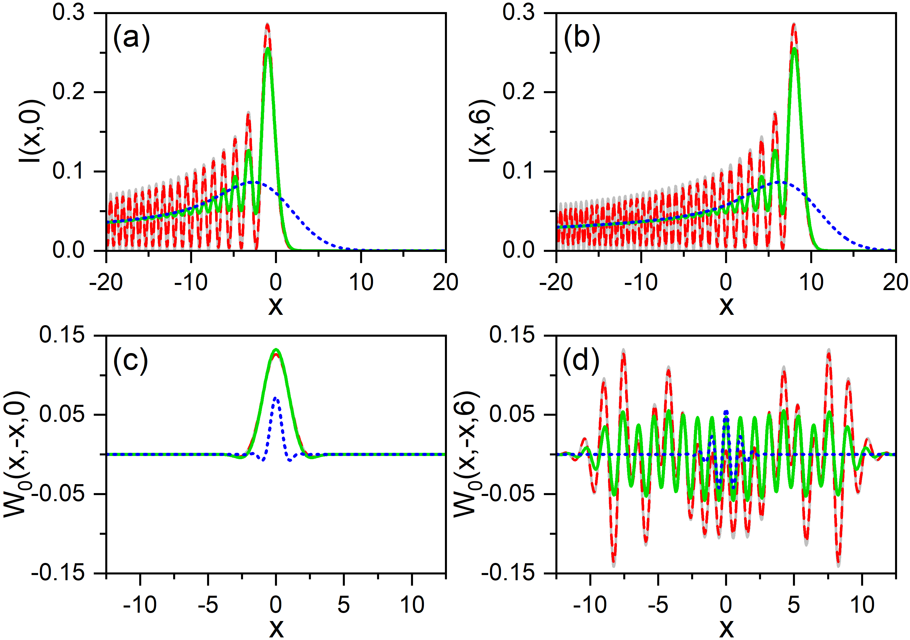
Figure 1: Partially coherent Airy beam affected by the spread function $P(\lambda)$ (23). The intensity distribution is displayed in the top panels, while the amplitude $\mathcal{W}_{0}$ is shown in the bottom ones for three different values of the spread parameter $\sigma$: $\sigma=0.1$ (dashed red line), $\sigma=0.5$ (solid green line), and $\sigma=5$ (dotted blue line). Both quantities have been computed at $z=0$ (left panels) and $z=6$ (right panels) in order to make more apparent the shape-invariance and self-acceleration properties that characterize this type of infinite energy beams, as well as the gradual suppression of the spatial correlations (measured through $\mathcal{W}_{0}$) as $\sigma$ increases. To compare with, the fully coherent case (thin solid gray line), corresponding to $P(\lambda)\sim\delta(\lambda)$, has also been included in all cases. [Note that we are using dimensionless units (see text for details) and hence no units are specified either in this figure or the following ones.]

To better understand the action of (23) over the coherence of the infinite energy Airy beam, consider the cases displayed in Fig. 1, where the intensity distribution is shown in the top panels [Figs. 1(a) and 1(b)], while the amplitude $\mathcal{W}_{0}(x,-x,z)$, with $x^{\prime}=-x$, is represented in the bottom ones [Figs. 1(c) and 1(d)]. Note that, to simplify the analysis, $\mathcal{W}_{0}(x,x^{\prime},z)$ has been considered instead of $\mathcal{W}(x,x^{\prime},z)$, which avoids the effect of the fast oscillations due to the the complex exponential prefactor in the latter. The fully coherent Airy beam (i.e., the usual Airy beam) is represented in all cases with the thin solid gray line. As it can be seen, comparing Figs. 1(a) and 1(b), for $z=0$ and $z=6$, respectively, the beam is shape invariant, with all points of the latter having undergone a displacement rightwards equivalent to $z^{2}/4=9$. Note how the leading maximum at $x_{\rm max}\approx-1$ [see Fig. 1(a)] has moved to $x_{\rm max}\approx 8$ [see Fig. 1(b)], which makes evident the characteristic self-acceleration, although the full-width at half maximum remains the same in both cases (${\rm FWHM}\approx 1.64$). However, regarding the space correlations of the beam, described by $\mathcal{W}_{0}$, the lower panels show a remarkable increase along the secondary diagonal ($x^{\prime}=-x$), determined by the development of long-range, fast oscillations. This can be understood as an effect of the spatial overlapping of larger and larger portions of an Airy beam traveling in one direction (say, positive $x$) with its mirror image, traveling in the opposite direction (towards negative $x$). Thus, at $z=0$, basically only the main lobes of both counter propagating beams overlap, giving rise to a single (and positive) “bump”, as seen in Fig. 1(c). However, at $z=6$, the effective overlapping covers, approximately, the region that goes from $x\approx-10$ to $x\approx 10$, thus giving rise to the fast oscillations within this range observed in Fig. 1(d).

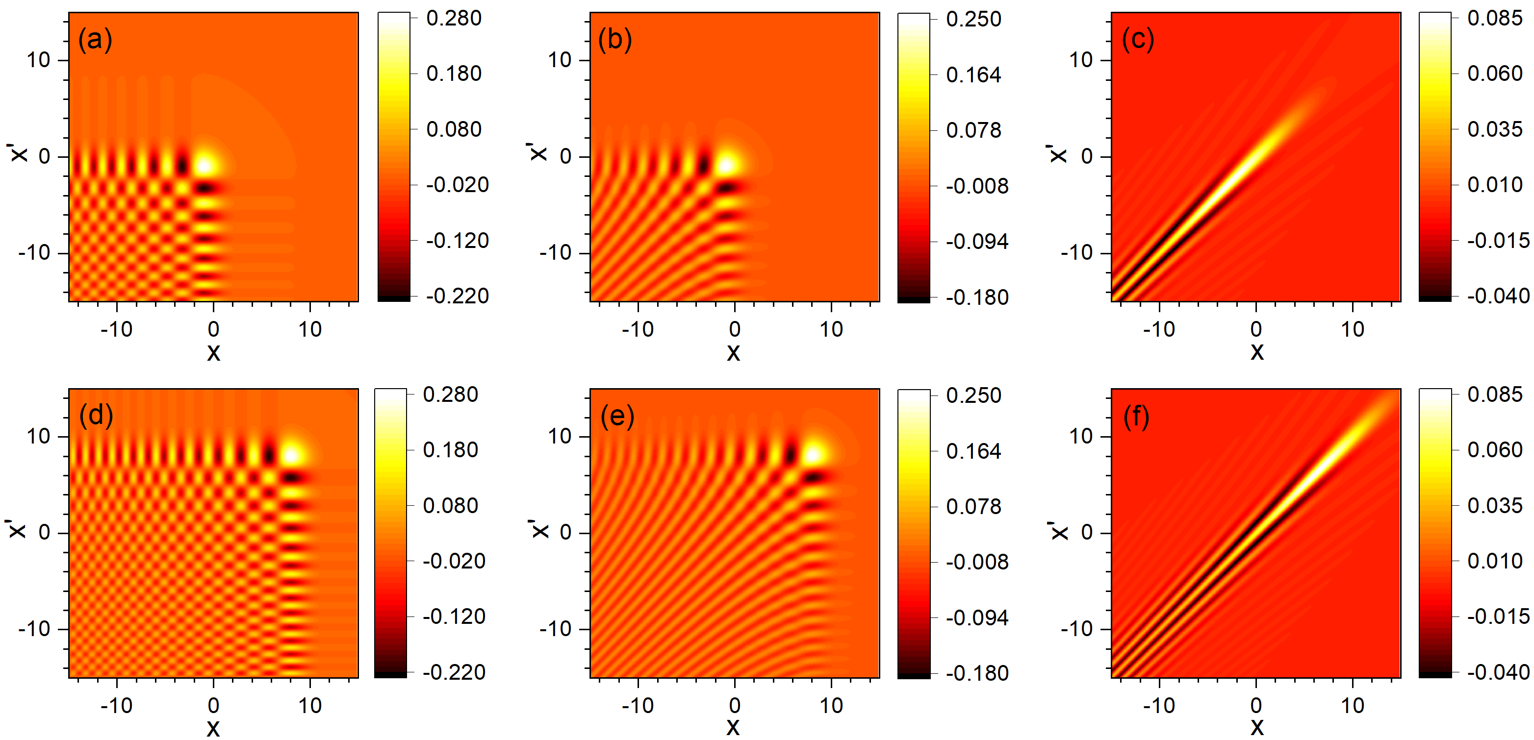
Figure 2: Density plots describing the behavior of the amplitude $\mathcal{W}_{0}(x,x^{\prime},z)$ for the three values of the spread parameter $\sigma$ considered above in Fig. 1: $\sigma=0.1$ (left column), $\sigma=0.5$ (middle column), and $\sigma=5$ (right column). To better perceive the shape invariance of the partially coherent beams and their self-acceleration, the same two cases for $z$ have also been considered: $z=0$ (top row) and $z=6$ (bottom row).

Let us now consider the effects of incoherence induced by (23). Thus, if $\sigma$ is small compared to the FWHM associated with the main lobe, this maximum as well as the nearby (on its left) maxima of the Airy beam will basically remain unaffected. The effect will start being noticed as the width of the maxima that form the tail of the beam become comparable with the value of $\sigma$. This is what can be observed for $\sigma=0.1$ (dashed red line in all panels in Fig. 1), particularly further away from the main lobe, as seen in Fig. 1(b), which translates into lower maxima and non-negligible minima. Regarding $\mathcal{W}_{0}$, though, no important effects can be noticed either at $z=0$ [see Fig. 1(c)] or at $z=6$ [see panel Fig. 1(d)], because within the $x$-range covered the Airy beam does not experience important incoherence effects [see Figs. 1(a) and 1(b)]. However, by further increasing the value of $\sigma$, to $\sigma=0.5$ (solid green line), the effect becomes more prominent, as seen in both top panels. For this value of $\sigma$, only the leading maximum remains, while the faint signature of few secondary maxima can also be perceived, approaching very quickly a decreasing tail. Correspondingly, the oscillations displayed by $\mathcal{W}_{0}$ also undergo a remarkable damping. Finally, in the regime of large $\sigma$, here illustrated with $\sigma=5$ (dotted blue line), we find no traits of interference at all; the whole intensity distribution has been smoothed out and now looks like the average value of the former Airy beam. Essentially, coherence has almost totally been washed out; the only living trait can be noticed through $\mathcal{W}_{0}$, with oscillations that remain pretty close to a small region around $x=0$, as seen in Fig. 1(d). Nevertheless, in all these partially coherent cases, neither the shape-invariance property nor the self-acceleration one disappear, but they are nicely preserved.

To better appreciate why in the large $\sigma$ range oscillations still persist in the CSD, thus indicating the presence of spatial correlations in this regime, while the intensity distribution looks like a distribution for a fully incoherence beam, in Fig. 2 we have represented, in terms of density plots, the amplitude $\mathcal{W}_{0}$ for the three values of $\sigma$ considered in Fig. 1 and the two values of $z$. Thus, from top to bottom, $\sigma=0.1$ (left column), $\sigma=0.5$ (middle column), and $\sigma=5$ (right column); on the top row, the density plots represent the cases for $z=0$, while on the bottom row, it is for $z=6$. As it can be read in the color code legend, on the right of each panel, the transition from negative to positive values is indicated with lighter and lighter shading. Again, all cases shown clear evidence of the already mentioned shape-invariance and self-acceleration properties regardless of $\sigma$, which indicates that these properties are not characteristic traits of fully coherent Airy beams, but they can also be observed in partially coherent Airy beams with infinite energy. Furthermore, these density plots show that the effect of (23) consists of annihilating the interferential (oscillatory) traits in a faster manner along the main diagonal (which coincides with the intensity distribution) than along the secondary diagonal, where there is a gradual “collapse” of $\mathcal{W}_{0}$ towards the main diagonal as $\sigma$ increases. This collapsing towards the main diagonal is, indeed, analogous to the effect that decoherence has on the density matrix that specifies the state of a quantum system, when the latter is influenced by a Markovian, Brownian-type environment [23].

Finally, it is also worth noting that the above family of CSDs can be further enlarged by adding a function $F(x^{\prime}-x)$ to the CSD (15) [24], i.e.,

$$\mathcal{W}_{F}(x,x^{\prime},z) = \mathcal{W}(x,x^{\prime},z)+F(x^{\prime}-x)$$ (24)

$$= e^{i(x^{\prime}-x)z/2}\ \!\mathcal{W}(x-z^{2}/4,x^{\prime}-z^{2}/4,0)$$

$$\qquad+F(x^{\prime}-x),$$

such that

$$F(x^{\prime}-x)=\int\tilde{\mathcal{F}}(\eta)e^{i(x^{\prime}-x)\eta}\ \!d\eta,$$ (25)

with

$$\tilde{\mathcal{F}}(\eta) > 0,$$ (26)

$$\int\tilde{\mathcal{F}}(\eta)\ \!d\eta \prec \infty,$$ (27)

With this gauge-type transformation, not only $\mathcal{W}_{F}(x,x^{\prime},z)$ is well-defined and satisfies the paraxial wave equation, but the intensity still remains shape-invariant. This can easily be shown as follows. From (24), we have

$$I_{F}(x,z)=I(x,z)+F(0).$$ (28)

where $F(0)$ is a constant with finite value, as it follows from the above properties for $\tilde{\mathcal{F}}(\eta)$. Thus, because $I(x,z)$ is shape-invariant, we find

$$I_{F}(x,z)=I_{F}(x-z^{2}/4,0).$$ (29)

On the contrary, the modulus of the complex degree of coherence (and hence other coherence-based quantities, such as the visibility) will be sensitive to this transformation. As it can be noted from (24), we have

$$|\mathcal{W}_{F}(x,x^{\prime},z)|^{2} = |\mathcal{W}(x,x^{\prime},z)|^{2}+|F(x^{\prime}-x)|^{2}+2{\rm Re}\left[F^{*}(x^{\prime}-x)\mathcal{W}(x,x^{\prime},z)\right]$$ (30)

$$= |\mathcal{W}(x-z^{2}/4,x^{\prime}-z^{2}/4,0)|^{2}+|F(x^{\prime}-x)|^{2}$$

$$+2{\rm Re}\left[e^{i(x^{\prime}-x)z/2}F^{*}(x^{\prime}-x)\mathcal{W}(x-z^{2}/4,x^{\prime}-z^{2}/4,0)\right].$$

On the other hand, we also have

$$|\mathcal{W}_{F}(x-z^{2}/4,x^{\prime}-z^{2}/4,0)|^{2} = |\mathcal{W}(x-z^{2}/4,x^{\prime}-z^{2}/4,0)|^{2}+|F(x^{\prime}-x)|^{2}$$ (31)

$$+2{\rm Re}\left[F^{*}(x^{\prime}-x)\mathcal{W}(x-z^{2}/4,x^{\prime}-z^{2}/4,0)\right].$$

Comparing both expressions, we reach the following result:

$$|\mathcal{W}_{F}(x,x^{\prime},z)|^{2}-|\mathcal{W}_{F}(x-z^{2}/4,x^{\prime}-z^{2}/4,0)|^{2} = 2{\rm Re}\left\{\left[e^{i(x^{\prime}-x)z/2}-1\right]F^{*}(x^{\prime}-x)\mathcal{W}(x-z^{2}/4,x^{\prime}-z^{2}/4,0)\right\}$$ (32)

$$= 4\sin\left[\frac{(x^{\prime}-x)z}{4}\right]$$

$$\quad\times{\rm Re}\left[ie^{i(x^{\prime}-x)z/4}F^{*}(x^{\prime}-x)\mathcal{W}(x-z^{2}/4,x^{\prime}-z^{2}/4,0)\right].$$

Taking into account that $\mathcal{W}(x-z^{2}/4,x^{\prime}-z^{2}/4,0)$ is a real quantity, the above expression can be recast as

$$|\mathcal{W}_{F}(x,x^{\prime},z)|^{2}-|\mathcal{W}_{F}(x-z^{2}/4,x^{\prime}-z^{2}/4,0)|^{2} = 4\sin\left[\frac{(x^{\prime}-x)z}{4}\right]$$

$$\quad\times\mathcal{W}(x-z^{2}/4,x^{\prime}-z^{2}/4,0)\ \!{\rm Im}\left[e^{-i(x^{\prime}-x)z/4}F(x^{\prime}-x)\right],$$

which shows that, in general, the shape-invariance is not preserved for the complex degree of coherence (4) for this family of CSDs, since

$$|\gamma_{F}(x,x^{\prime},z)|\neq|\gamma_{F}(x-z^{2}/4,x^{\prime}-z^{2}/4,0)|.$$ (34)

Therefore, concerning the preservation of quantities such as the modulus of the degree of coherence or the which-path distinguishability, the use of infinite-energy partially coherence beams described by the CSD (15) is mandatory.

III Finite Energy Beams

The partially coherent beams introduced in Sec. II correspond to ideal situations that are no experimentally accessible in the laboratory. Let us then investigate the feasibility of finite-energy partially coherent beams that nearly preserve all properties of the infinite-energy ones seen above. In this regard, two types of partially coherent beams are introduced with finite energy and hence experimentally feasible. To this end, some specific correlations among the displacements acting on the random field amplitude realizations are considered, thus extending the CSD functional form obtained in Sec. II.

In order to determine to what extent the above mentioned finite-energy partially coherent beams keep the shape invariance as they propagate along $z$, we introduce a measure of the overlapping or projection of the corresponding partially coherent CSD at that $z$-plane, $\mathcal{W}_{i0}(x,x^{\prime},z)$ ($i={\rm I},{\rm II}$ labels the respective CSD type) with the input CSD shifted along the transverse direction a distance $z^{2}/4$, $\mathcal{W}_{i0}(x-z^{2}/4,x^{\prime}-z^{2}/4,0)$,

$$\varepsilon_{i}(z)=\frac{\displaystyle\left\arrowvert\iint\mathcal{W}_{i,0}^{*}(x-z^{2}/4,x^{\prime}-z^{2}/4,0)\mathcal{W}_{i,0}(x,x^{\prime},z)\right\arrowvert^{2}dxdx^{\prime}}{\displaystyle\iint\left\arrowvert\mathcal{W}_{i,0}(x-z^{2}/4,x^{\prime}-z^{2}/4,0)\right\arrowvert^{2}dxdx^{\prime}\ \iint\left\arrowvert\mathcal{W}_{i,0}(x,x^{\prime},z)\right\arrowvert^{2}dxdx^{\prime}},$$ (35)

which satisfies $0\leq\varepsilon_{i}(z)\leq 1$. If $\mathcal{W}_{i0}(x,x^{\prime},z)$ remains relatively shape-invariant, that is, resembling the shifted CSD, $\mathcal{W}_{i0}(x-z^{2}/4,x^{\prime}-z^{2}/4,0)$, then $\varepsilon_{i}(z)$ will be close to the unity, because there will be an important overlapping between both amplitudes. On the the contrary, if finite-energy effects are relevant, then the behavior of both CSDs will divert very quickly, in relatively short distances $z$, and hence $\varepsilon_{i}(z)$ will exhibit a fast falloff to zero with $z$.

III.1 Type-I CSD

The first type of beams are such that, at the input plane $z=0$, their CSD is given by

$$\mathcal{W}_{\rm I}(x,x^{\prime},0)=\iint\mathcal{C}_{I}(\lambda,\lambda^{\prime})Ai(x-\lambda)Ai(x^{\prime}-\lambda^{\prime})\ \!d\lambda d\lambda^{\prime},$$ (36)

in analogy to Eq. (LABEL:eq9), with

$$\mathcal{C}_{I}(\lambda,\lambda^{\prime})=\mathcal{P}(\lambda,\lambda^{\prime})\mathcal{Q}(\lambda-\lambda^{\prime}),$$ (37)

which must be a non-negative definite Hermitian function. The above two correlation functions (bivariate distributions) are required to satisfy the conditions

$$\mathcal{Q}(0) \prec \infty,$$ (38)

$$\int\mathcal{P}(\lambda,\lambda)\ \!d\lambda \prec \infty,$$ (39)

for $\mathcal{W}_{\rm I}(x,x^{\prime},0)$ to be well-defined and to carry finite energy. Note that, in the particular case

$$\mathcal{Q}(\lambda-\lambda^{\prime})\sim\delta(\lambda-\lambda^{\prime}),$$ (40)

the CSD (36) will be close to the infinite energy CSD (LABEL:eq9), thus exhibiting analogous properties to the latter. As for the propagated form of Eq. (36), following the prescription given in Sec. II, we find

$$\mathcal{W}_{\rm I}(x,x^{\prime},z)=e^{i(x^{\prime}-x)z/2}\mathcal{W}_{{\rm I},0}(x,x^{\prime},z),$$ (41)

with

$$\mathcal{W}_{{\rm I},0}(x,x^{\prime},z) = \iint\mathcal{C}_{\rm I}(\lambda,\lambda^{\prime})e^{i(\lambda-\lambda^{\prime})z/2}Ai(x-\lambda-z^{2}/4)$$ (42)

$$\qquad\times Ai(x^{\prime}-\lambda^{\prime}-z^{2}/4)\ \!d\lambda d\lambda^{\prime}.$$

Note that, due to the correlation between $\lambda$ and $\lambda^{\prime}$, now it is not possible to ensure that the propagated solution is either shape invariant or self-accelerating.

To further investigate this type of CSDs, let us now assign a functional form to the bivariate distributions $\mathcal{P}$ and $\mathcal{Q}$ satisfying the above requirements and, at the same time, that are analogous to functional forms that can be found in the literature for CSDs similar to the one defined by Eq. (36) [25]. Accordingly, consider

$$\mathcal{P}(\lambda,\lambda^{\prime}) = e^{-\alpha(\lambda^{2}+\lambda^{\prime 2})},$$ (43)

$$\mathcal{Q}(\lambda-\lambda^{\prime}) = e^{-\beta(\lambda-\lambda^{\prime})^{2}},$$ (44)

from which we obtain

$$\mathcal{C}_{\rm I}(\lambda,\lambda^{\prime})=e^{-\alpha(\lambda^{2}+\lambda^{\prime 2})}e^{-\beta(\lambda-\lambda^{\prime})^{2}}.$$ (45)

Regarding $\mathcal{P}$, it accounts for the separate effect of the point spread functions associated with the random displacements $\lambda$ and $\lambda^{\prime}$, each given by a Gaussian distribution, like (23), with $\alpha$ determining the spread range or width of the distribution. On the other hand, $\mathcal{Q}$ introduces the correlation between $\lambda$ and $\lambda^{\prime}$, controlled by means of a $\beta$ parameter, such that, as $\beta$ gets larger and larger, $\mathcal{Q}$ approaches the aforementioned Dirac $\delta$ distribution. For computational convenience, to establish a better comparison among different cases in the results shown below, we are going to introduce a multiplicative normalizing prefactor $\mathcal{N}_{\rm I}$ in $\mathcal{W}_{\rm I}(x,x^{\prime},z)$, which arises from considering

$$\iint\mathcal{C}_{\rm I}(\lambda,\lambda^{\prime})\ \!d\lambda d\lambda^{\prime}=1.$$ (46)

This prefactor, which reads as

$$\mathcal{N}_{\rm I}=\frac{\sqrt{\alpha(\alpha+2\beta)}}{\pi},$$ (47)

has thus been considered in the numerical calculations involving both $\mathcal{W}_{\rm I}$ and the associated intensity, $I_{\rm I}(x,z)$, shown and discussed below.

Taking into account the above expressions for $\mathcal{P}$ and $\mathcal{Q}$, let us now investigate how the amplitude of the CSD (41), $\mathcal{W}_{{\rm I},0}(x,x^{\prime},z)$, deviates from a shape-invariant and self-accelerating behavior, described by the amplitude corresponding to moving a distance $z^{2}/4$ in both $x$ and $x^{\prime}$ the amplitude of the CSD (36). Thus, substituting the amplitudes of both (41) and (36) into Eq. (35) leads to

$$\varepsilon_{\rm I}(z)=\frac{\displaystyle\left\arrowvert\iint\left\arrowvert\mathcal{C}_{\rm I}(\lambda,\lambda^{\prime})e^{i(\lambda-\lambda^{\prime})z/2}\right\arrowvert^{2}\ \!d\lambda d\lambda^{\prime}\right\arrowvert^{2}}{\displaystyle\left[\iint\left\arrowvert\mathcal{C}_{\rm I}(\lambda,\lambda^{\prime})\ \!d\lambda d\lambda^{\prime}\right\arrowvert^{2}\right]^{2}}.$$ (48)

Substituting Eqs. (43) and (44) into this expression leads to

$$\varepsilon_{\rm I}(z)=e^{-z^{2}/(8\alpha+16\beta)},$$ (49)

which depends on the parameters describing the spread of both distributions. In other words, the correlation between displacements is, in principle, at the same level in relevance as the independent spread functions, unless one of them clearly prevails over the other (which can be done by properly tuning $\alpha$ and $\beta$). Furthermore, also note that (49) also introduces a scale along the $z$-direction

$$z_{\rm I}=\sqrt{8(\alpha+2\beta)},$$ (50)

such that, when $z=z_{\rm I}$, the overlapping between the two amplitudes reduces to about 37%. This means that the fidelity between both amplitudes, and hence the preservation of the two Airy-beam properties, will be guaranteed for $z\ll z_{\rm I}$, while the propagated amplitude will lose these traits as $z$ increases (particularly, for $z\gg z_{\rm I}$).

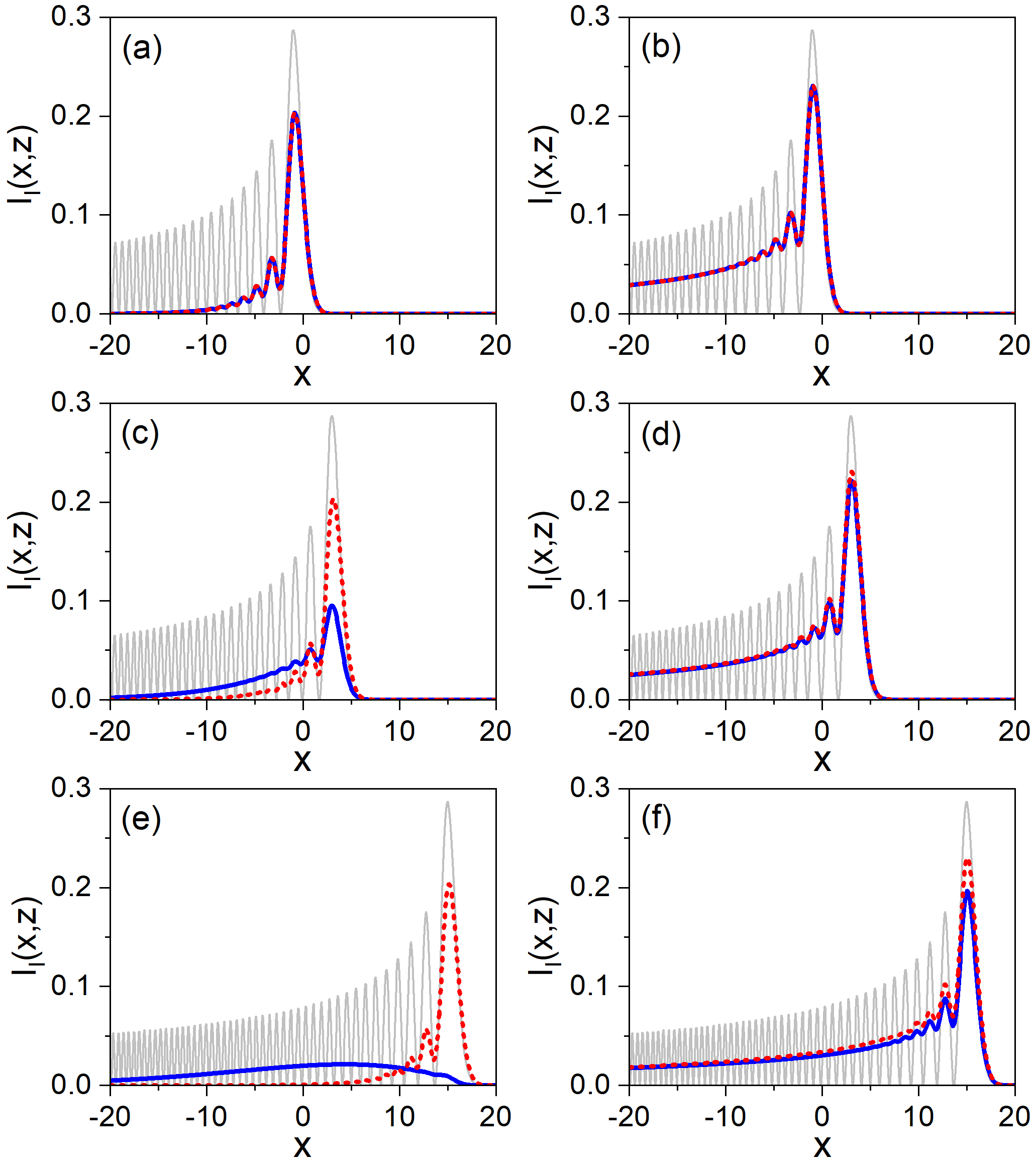
Figure 3: Intensity distribution $I_{\rm I}(x,z)$ for $\alpha=1$ and: $\beta=0.5$ (left column) and $\beta=24.5$ (right column). In each panel, $I_{\rm I}(x,z)$ is denoted with the solid blue line, while the dotted red line represents $I_{\rm I}(x-z^{2}/4,0)$; to compare with, the intensity of the fully coherent Airy beam is also included (thin solid gray line). From top to bottom: $z=0$, $z=4$, and $z=8$.

Figures 3 and 4 show, respectively, the intensity and the amplitude $\mathcal{W}_{{\rm I},0}$, with $x^{\prime}=-x$, for different values of $z$ (increasing from top to bottom) and two values of the parameter $\beta$. In all graphs, the same value $\alpha=1$ is considered, such that Eq. (43) corresponds to a Gaussian distribution of width $\sigma=1$, i.e., in the intermediate range of coherence, following the results discussed in Sec. II). Regarding the values assigned to $\beta$, they have been chosen taking into account the discussion about $z_{\rm I}$. Specifically, we have considered $\beta=0.5$ and 24.5, for which $z_{\rm I}=4$ and 20, respectively. If we compare the intensity distributions displayed in Figs. 3(a) and 3(b), for $z=0$, we find that the overall profile is essentially determined by $\alpha$ (similar damped oscillatory behavior in both cases, compared to the fully coherent Airy beam, denoted with the thin solid gray line), but the reach is longer in the case of larger $\beta$. Accordingly, it is clear that, while $\mathcal{P}$ rules the partial coherence of the beam, the distribution $\mathcal{Q}$ is going to determine the energy content. On the other hand, as indicated above regarding the physical meaning of $z_{\rm I}$, by inspecting Figs. 3(c) and 3(d), for $z=4$, and Figs. 3(e) and 3(f), for $z=8$, we readily notice that the statement is correct, as the intensity for larger $\beta$ (i.e., $\beta=24.5$) basically preserves the shape-invariance and self-accelerating properties for the $z$-range considered, while the same does not happen for small $\beta$. In the latter case, not only the coherence is remarkably lost at $z=2$, but the intensity distribution (solid blue line) is smeared out all over the place as $z$ further increases, thus loosing all information about the initial profile, which becomes unrecognizable compared to the simply displaced intensity distribution (dotted red line).

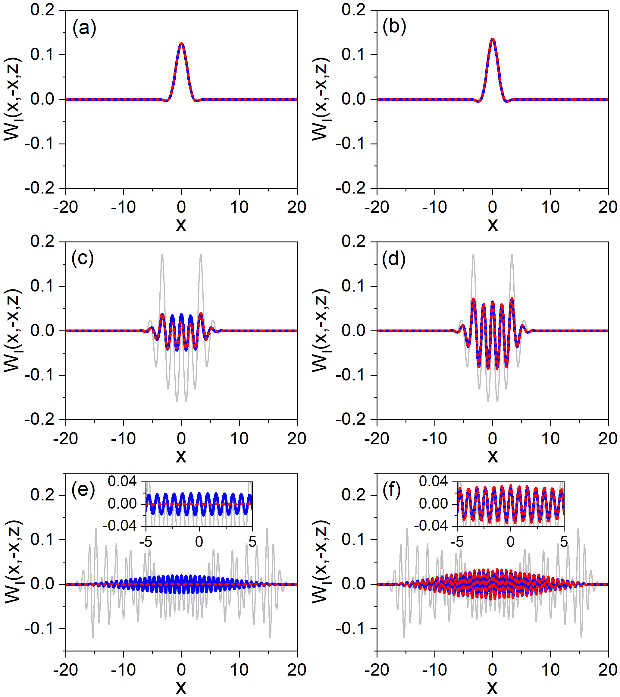
Figure 4: Function $\mathcal{W}_{{\rm I},0}(x,-x,z)$ for $\alpha=1$ and: $\beta=0.5$ (left column) and $\beta=24.5$ (right column). In each panel, $\mathcal{W}_{{\rm I},0}(x,-x,z)$ is denoted with the solid blue line, while the dotted red line represents $\mathcal{W}_{{\rm I},0}(x-z^{2}/4,-x-z^{2}/4,0)$; to compare with, the intensity of the fully coherent Airy beam is also included (thin solid gray line). From top to bottom: $z=0$, $z=4$, and $z=8$. The insets in panels (e) and (f) provide an enlarged view of the central part of the amplitudes to better appreciate the deviations among them.

Regarding the coherence properties exhibited by the CSD, let us now focus on Fig. 4. As it is shown for $\beta=0.5$ (see left column, from top to bottom), the oscillatory behavior of the CSD evaluated at $x^{\prime}=-x$ (solid blue line) is relatively weak compared to the fully coherent case (thin solid gray line), particularly at $z=8$ [see Fig. 4(f)]. Although the intensity profile is rather unstructured (it resembles an asymmetric Gaussian), the fact that it spans a relatively long distance ensures that the overlapping integral (42) does not vanish for a similar range, which warrants the permanence of the oscillatory behavior in distances comparable with those covered by the fully coherent case. Note that, on the contrary, if the displaced distribution is considered (see dotted red line), because of its faster falloff (and hence a robust overlapping over much shorter distances), such oscillatory behavior has already disappeared for $z=8$, where we observe a nearly flat CSD [see Fig. 4(f)]. This behavior is in contrast with what happens in the case of larger $\beta$ (see right column), where both CSDs, the propagated one (solid blue line) and the displaced one (dotted red line), exhibit basically the same behavior, because the overlapping integral is nonzero over a larger distance in the second case, as a consequence of the shorter range of $\mathcal{Q}$. Of course, there is still a gradual cancellation of the oscillations as $x$ increases in both cases, but note that this arises from the smoothing produced by the $\mathcal{P}$ distribution.

III.2 Type-II CSD

Concerning the second type of beam, we define its CSD as follows

$$\mathcal{W}_{\rm II}(x,x^{\prime},0)=\int\mathcal{R}(\lambda^{\prime\prime})S^{*}(x-\lambda^{\prime\prime})S(x^{\prime}-\lambda^{\prime\prime})\ \!d\lambda^{\prime\prime},$$ (51)

which is well defined if $\mathcal{R}(\lambda)>0$, and where

$$S(x)=\int\tilde{\mathcal{S}}(\lambda)Ai(x-\lambda)\ \!d\lambda$$ (52)

describes a finite-energy Airy beam [24, 25, 26, 27, 28, 29] if

$$\iint\mathcal{R}(\lambda^{\prime\prime})|\tilde{\mathcal{S}}(\lambda-\lambda^{\prime\prime})|^{2}\ \!d\lambda d\lambda^{\prime\prime}<\infty.$$ (53)

Making explicit the substitution of (52) into the CSD (51), we obtain

$$\mathcal{W}_{\rm II}(x,x^{\prime},0) = \iiint\mathcal{R}(\lambda^{\prime\prime})\tilde{\mathcal{S}}^{*}(\mu)\tilde{\mathcal{S}}(\mu^{\prime})Ai(x-\mu-\lambda^{\prime\prime})$$

$$\qquad\quad\times Ai(x^{\prime}-\mu^{\prime}-\lambda^{\prime\prime})\ \!d\mu d\mu^{\prime}d\lambda^{\prime\prime}$$

$$= \iint\mathcal{C}_{\rm II}(\lambda,\lambda^{\prime})Ai(x-\lambda)Ai(x^{\prime}-\lambda^{\prime})\ \!d\lambda d\lambda^{\prime},$$

with

$$\mathcal{C}_{\rm II}(\lambda,\lambda^{\prime\prime})=\int\mathcal{R}(\lambda^{\prime\prime})\tilde{\mathcal{S}}^{*}(\lambda-\lambda^{\prime\prime})\tilde{\mathcal{S}}(\lambda^{\prime}-\lambda^{\prime\prime})\ \!d\lambda^{\prime\prime},$$ (55)

in analogy to Eq. (LABEL:eq9), and where we have made use of the identity

$$\int\tilde{\mathcal{S}}(\mu)Ai(x-\mu-\lambda^{\prime\prime})\ \!d\mu=\int\tilde{\mathcal{S}}(\lambda-\lambda^{\prime\prime})Ai(x-\lambda)\ \!d\lambda,$$ (56)

on the right-hand side of the second equality in Eq. (LABEL:eq30b), with $\lambda=\mu+\lambda^{\prime\prime}$ [a similar expression holds for the terms depending on $\mu^{\prime}$ in (LABEL:eq30b), with $\lambda^{\prime}=\mu^{\prime}+\lambda^{\prime\prime}$]. Despite the apparently complicated functional form displayed by (LABEL:eq30b), the fact that it represents a finite energy beam can readily be seen by integrating over $x$ the associated intensity distribution. After integration, one obtains the total power described by the expression (53), which is bound (finite). Actually, if a Gaussian distribution is chosen for $\tilde{\mathcal{S}}$, then the finite-energy Airy beam introduced in Ref. [26] is recovered.

Following the same procedure as before, we find that the propagated form of the CSD (51) reads as

$$\mathcal{W}_{\rm II}(x,x^{\prime},z)=e^{i(x^{\prime}-x)z/2}\mathcal{W}_{{\rm II},0}(x,x^{\prime},z),$$ (57)

with

$$\mathcal{W}_{{\rm II},0}(x,x^{\prime},z) = \iint\mathcal{C}_{\rm II}(\lambda,\lambda^{\prime})e^{i(\lambda-\lambda^{\prime})z/2}Ai(x-\lambda-z^{2}/4)$$ (58)

$$\qquad\times Ai(x^{\prime}-\lambda^{\prime}-z^{2}/4)\ \!d\lambda d\lambda^{\prime}.$$

Equation (57) thus paves an alternative way to build partially coherent Airy beams with finite energy.

To further investigate the behavior of this type of CSD, let us now consider some particular functional forms for both $\mathcal{R}$ and $\tilde{\mathcal{S}}$. More specifically, as in the previous cases analyzed, we also consider Gaussian distributions, i.e.,

$$\mathcal{R}(u) = e^{-au^{2}},$$ (59)

$$\tilde{\mathcal{S}}(v) = e^{-bv^{2}}.$$ (60)

As before, also for computational convenience, to set a comparison between difference cases below, we consider

$$\iint\mathcal{C}_{\rm II}(\lambda,\lambda^{\prime})\ \!d\lambda d\lambda^{\prime}=1,$$ (61)

which renders the renormalization prefactor

$$\mathcal{N}_{\rm II}=\frac{b}{\pi}\sqrt{\frac{a}{a+2b}}.$$ (62)

It is worth mentioning, though, that with the choice (59) and (60), $\mathcal{C}_{\rm II}$ acquires a similar functional form to Eq. (45) for $\mathcal{C}_{\rm I}$ in terms of the distributions (43) and (44), namely,

$$\mathcal{C}_{\rm II}(\lambda,\lambda^{\prime})=e^{-\alpha^{\prime}(\lambda^{2}+\lambda^{\prime 2})}e^{-\beta^{\prime}(\lambda-\lambda^{\prime})^{2}},$$ (63)

with

$$\alpha^{\prime} = \frac{ab}{a+2b},$$ (64)

$$\beta^{\prime} = \frac{b^{2}}{a+2b}.$$ (65)

However, as it can be noticed, unlike $\mathcal{C}_{\rm I}$, here the spread factors, $\alpha^{\prime}$ and $\beta^{\prime}$, involve features from both (59) and (60). In other words, although each Airy beam is independently affected by a spread function $\tilde{\mathcal{S}}$, the effect of $\mathcal{R}$ is to set a correlation between $\lambda$ and $\lambda^{\prime}$.

Two limits can be clearly identified. For $a\gg b$, we obtain $\alpha^{\prime}\approx b$ and $\beta^{\prime}\approx b^{2}/a\ll b$. Physically, this means that the spread range for $\lambda^{\prime\prime}$ is rather short and hence we are going to observe nice oscillations in the corresponding intensity distribution, although with a limited spatial extension. On the other hand, for $a\ll b$, we find $\alpha^{\prime}\approx a/2$ and $\beta^{\prime}\approx b/2$, that is, the two exponential factors in $\mathcal{C}_{\rm II}$ describe independent distributions, as in the case of type-I CSDs. In this case, because $|\lambda-\lambda^{\prime}|$ can be relatively large, the oscillations typical of the Airy function are expected to be partially suppressed (depending on the actual value of the parameters $a$ and $b$).

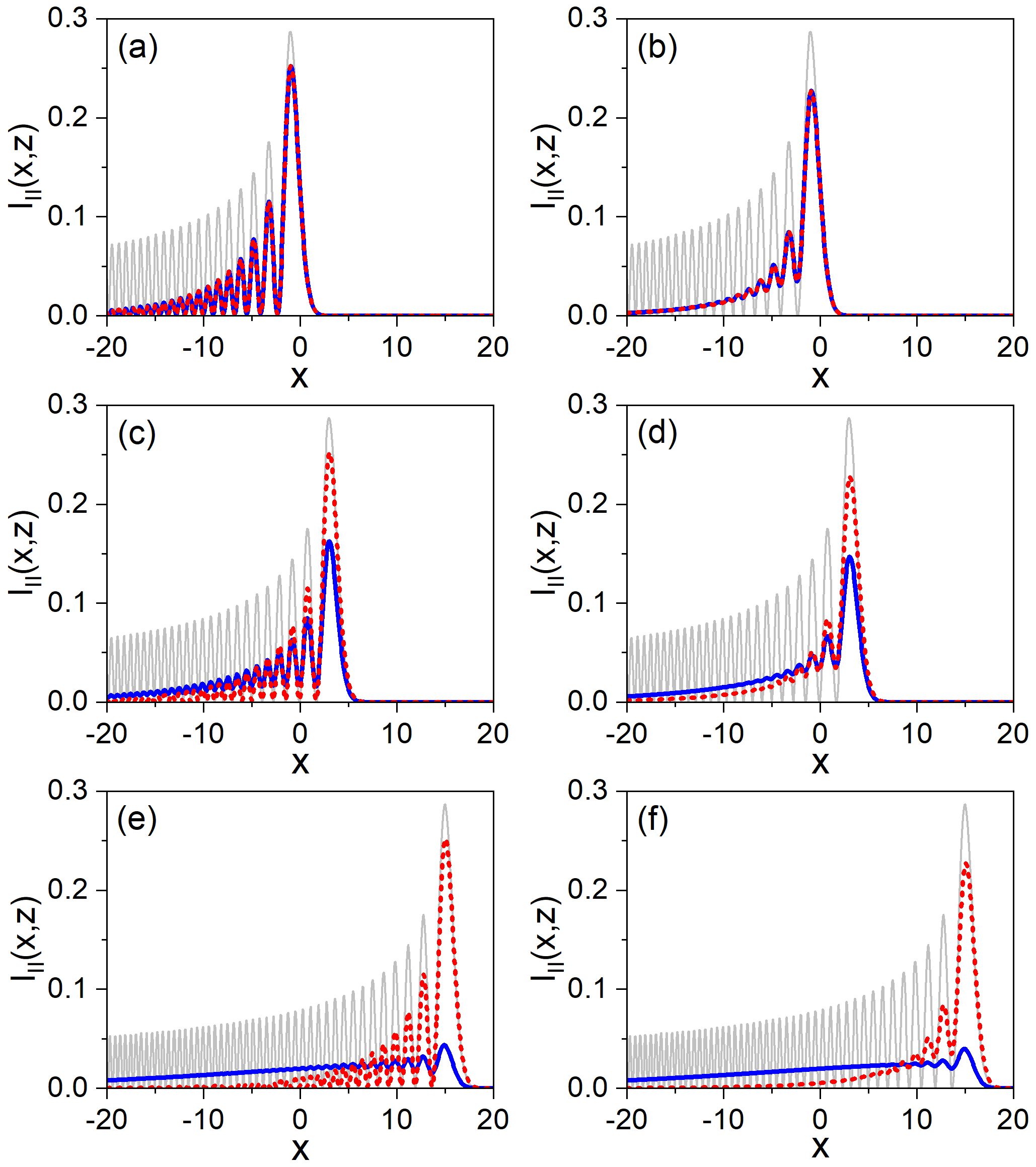
Figure 5: Intensity distribution $I_{\rm II}(x,z)$ for $a=4$ and: $b=1$ (left column) and $b=5$ (right column). In each panel, $I_{\rm II}(x,z)$ is denoted with the solid blue line, while the dotted red line represents $I_{\rm II}(x-z^{2}/4,0)$; to compare with, the intensity of the fully coherent Airy beam is also included (thin solid gray line). From top to bottom: $z=0$, $z=4$, and $z=8$.

Here, the expression (35) for the overlapping between the CSD (58) and the CSD (LABEL:eq30b) propagated to the output plane $z$, reads as

$$\varepsilon_{\rm II}(z)=\frac{\displaystyle\left\arrowvert\iint\left\arrowvert\mathcal{C}_{\rm II}(\lambda,\lambda^{\prime})\right\arrowvert^{2}e^{i(\lambda-\lambda^{\prime})z/2}d\lambda d\lambda^{\prime}\right\arrowvert^{2}}{\displaystyle\left[\iint\left\arrowvert\mathcal{C}_{\rm II}(\lambda,\lambda^{\prime})\right\arrowvert^{2}d\lambda d\lambda^{\prime}\right]^{2}}.$$ (66)

After substituting (63) into this expression, we find

$$\varepsilon_{\rm II}(z)=e^{-z^{2}/16b}.$$ (67)

which only depends on $b$, unlike the correlation function $\mathcal{C}_{\rm II}$, Eq. (63), which depends on both parameters. In this regard, each $b$ parameter determines a whole family of finite energy, partially coherent beams, as all of them are going to behave the same way, although with different degrees of incoherence, which is essentially governed by the $a$ parameter. Furthermore, each of these families obeys to the same decay length scale,

$$z_{\rm II}=4\sqrt{b},$$ (68)

i.e., regardless of the degree of coherence imposed by $a$, for all type-II beams the degradation of the shape-invariance and self-acceleration properties are specified by the same value of $z_{\rm II}$.

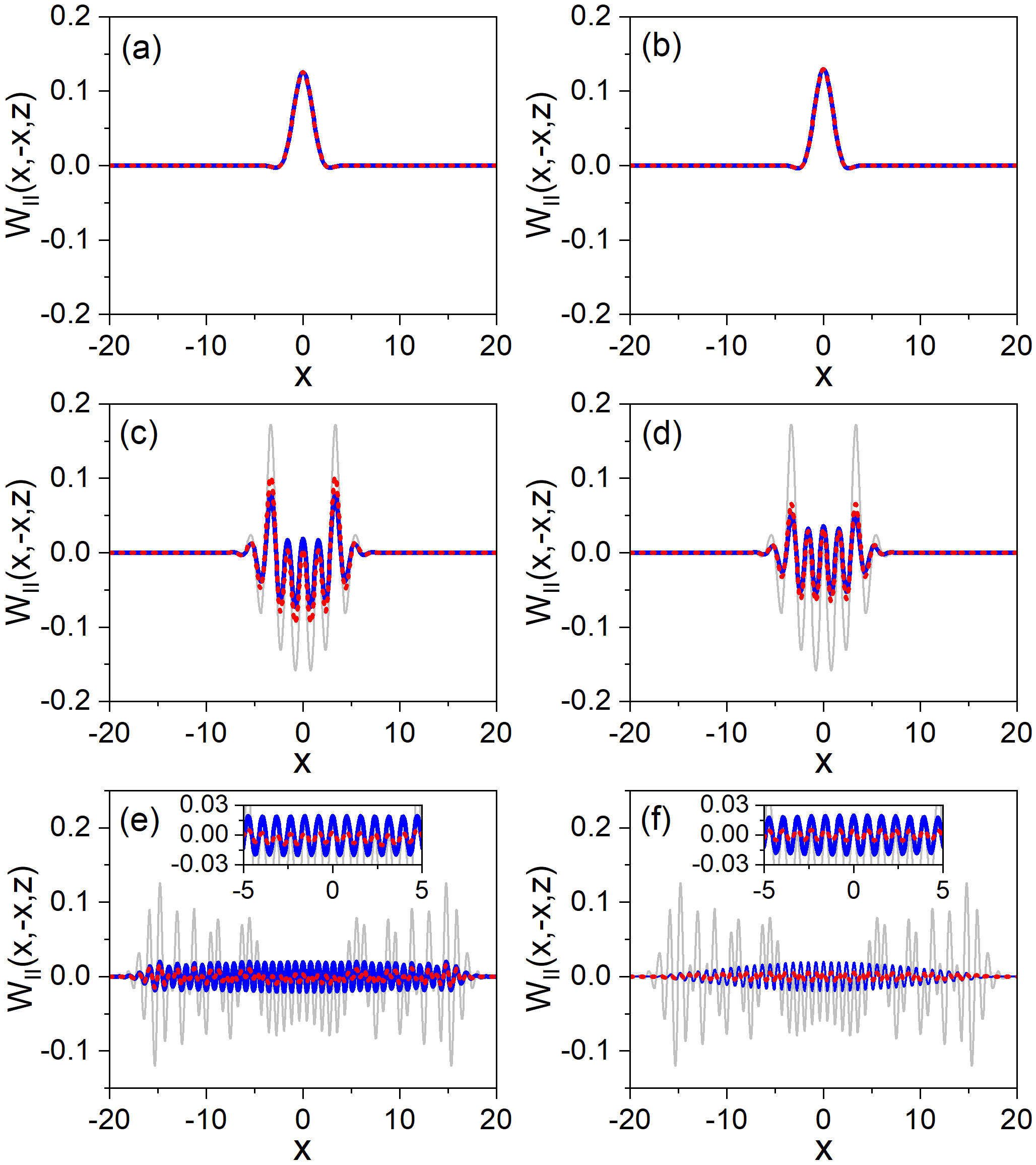
Figure 6: Function $\mathcal{W}_{{\rm II},0}(x,-x,z)$ for $a=4$ and: $b=1$ (left column) and $b=5$ (right column). In each panel, $\mathcal{W}_{{\rm II},0}(x,-x,z)$ is denoted with the solid blue line, while the dotted red line represents $\mathcal{W}_{{\rm II},0}(x-z^{2}/4,-x-z^{2}/4,0)$; to compare with, the intensity of the fully coherent Airy beam is also included (thin solid gray line). From top to bottom: $z=0$, $z=4$, and $z=8$. The insets in (e) and (f) provide with an enlarged view of the central part of $\mathcal{W}_{{\rm II},0}(x,-x,z)$ and $\mathcal{W}_{{\rm II},0}(x-z^{2}/4,-x-z^{2}/4,0)$ to better appreciate the deviations between them.

To better understand the above statement, in the intensity distribution for two type-II beams with the same $b$ but different values of $a$ and at different $z$-planes (with $z$ increasing from top to bottom) is shown in Fig. 5. In particular, we have chosen $b=4$, for which $z_{\rm II}=8$. Accordingly, the intensity distributions have been determined at $z=0$ (top), $z=4$ (middle), and $z=8$ (bottom) for $a=100$ (left column) and $a=4$ (right column), these two values being in compliance with the limiting situations discussed above. In particular, as seen in Figs. 5(a) and 5(b), $a=100$ represents a situation of high coherence, while $a=4$ describes a scenario with an important suppression of coherence, analogous to the cases analyzed in Sec. III.1. Moreover, also as in the previously analyzed case, the exponential-type decay tail, and hence the energy content of the beam, is determined by $b$. In order to get a better idea on the decrease of both coherence and energy, compare the results for the two cases, $a=100$ and $a=4$, with the fully coherent Airy beam (thin solid gray line). Now, as $z$ increases, it can also be seen that the overlapping between the type-II beams and the corresponding initial amplitudes moved rightwards by a quantity $z^{2}/4$ (dotted red line) decreases in a similar manner, in compliance with (67). In Figs. 5(c) and 5(d), for $z=4$ ($=z_{\rm II}/2$), the correspondence between both amplitudes falls to about 78%, so both shape invariance and self-acceleration can still be properly seen (although some deviations along the decaying tail can also be observed). However, in Figs. 5(e) and 5(f), for $z=8$ ($=z_{\rm II}$), such correspondence is much weaker, since the overlapping has fallen to about 37%. In this case, for both values of $a$, we can see that the beam has got a nearly homogeneous distribution all over the place.

In Fig. 6 we have represented the amplitude $\mathcal{W}_{{\rm II},0}$ along the secondary diagonal ($x^{\prime}=-x$). The results are pretty similar for both cases, with a rather homogeneous oscillatory structure within the region covered by the beam. Of course, in the case of shorter $a$, there is a faster decay towards the borders of $\mathcal{W}_{{\rm II},0}$, as seen above for type-II CSDs.

IV Concluding remarks

Over recent years, different methods have been considered in the literature to generate finite-energy coherent beams, which recreate the behavior of ideal Airy beams to a great extent. Some methods are based on the truncation of the angular momentum, which also induce incoherence by removing and/or acting on some of the beam spectral components. This has thus redirected the attention towards the design and experimental implementation of partially coherent Airy beams, because of their intrinsic interest as a new resource of structured light with important potential applications. Unlike previous approaches considered in the literature, here we have focused on exploiting the properties of the cross-spectral density (CSD) as an alternative strategy. Thus, we have analyzed its behavior when incoherence is added by assuming an action from external random fluctuations at the input plane. In this regard, it has been seen that the shape-invariance and self-acceleration properties displayed by fully coherent Airy beams can still be preserved in partially coherent Airy beams provided they carry infinite energy and the fluctuations that affect the field amplitude are totally uncorrelated.

From that starting point, by adding a certain correlation between the random fluctuations, we have been able to design two types of partially coherent beams with finite energy, which may display both shape-invariance and self-acceleration within a given range of the propagation distance, $z$, before such properties are totally lost. This $z$ range has been shown to depend on the parameter that specifies the distribution of fluctuations. Actually, this has been possible by defining a position-dependent parameter that quantifies the degree of overlapping between the propagated beam and the input one displaced by an amount equivalent to the propagation distance. As it has been shown, depending on how the correlations between random displacements are established, two types of CSDs have been introduced, for which this overlapping parameter exhibits a Gaussian-type decay. In what we have denoted as type-I CSD, the correlation among displacements is set on a local level, i.e., directly applied between two any different Airy beams. In this case, it has been seen that the decay rate depends on both the spread of the random displacements and the spread range of the correlations between two any random displacements. However, if the correlations are set on a nonlocal level, i.e., they affect a whole swarm of Airy beams that contribute to $S(x)$, then it has been shown that the decay rate only depends on the spatial extent of the spread range of the spectral correlation function $\tilde{\mathcal{S}}$. This is the case for what we have denoted as type-II CSDs. Note that, although in both cases one can determine how far the beam can be propagated with its Airy-type properties being mostly preserved, the simpler dependence of type-II CSDs on a single parameter enables the generation of an infinite family of partially coherent Airy-type beams all behaving the same way regarding shape invariance and self-acceleration.

Finally, it is also worth mentioning that all the theory here developed can be applied to the field of structured light beams as well as to the field of matter waves and wave-packet design. In this case, not only conditions for the design of particular particle beams are provided, but such conditions can also be used to established the extent of external factors that may act on the beams, leading to a suppression of their coherence properties (induced either by incoherence or by decoherence).

References

- Berry and Balazs [1979] M. V. Berry and N. L. Balazs, Nonspreading wave packets, Am. J. Phys. 47, 264 (1979).
- Greenberger [1980] D. M. Greenberger, Comment on “Nonspreading wave packets”, Am. J. Phys. 48, 256 (1980) .
- Unnikrishnan and Rau [1996] K. Unnikrishnan and A. R. P. Rau, Uniqueness of the Airy packet in quantum mechanics, Am. J. Phys. 64, 1034 (1996).
- Besieris et al. [1994] I. M. Besieris, A. M. Shaarawi, and R. W. Ziolkowski, Nondispersive accelerating wave packets, Am. J. Phys. 62, 519 (1994) .
- Goutsoulas and Efremidis [2021] M. Goutsoulas and N. K. Efremidis, Dynamics of self-accelerating electron beams in a homogeneous magnetic field, Phys. Rev. A 103, 013519 (2021).
- Pethick and Smith [2008] C. J. Pethick and H. Smith, Bose–Einstein Condensation in Dilute Gases (Cambridge University Press, Cambridge, 2008).
- Efremidis et al. [2013] N. K. Efremidis, V. Paltoglou, and W. von Klitzing, Accelerating and abruptly autofocusing matter waves, Phys. Rev. A 87, 043637 (2013).
- Yuce [2015] C. Yuce, Self-accelerating matter waves, Modern Physics Letters B 29, 1550171 (2015) .
- Fu et al. [2015] S. Fu, Y. Tsur, J. Zhou, L. Shemer, and A. Arie, Propagation dynamics of Airy water-wave pulses, Phys. Rev. Lett. 115, 034501 (2015).
- Rozenman et al. [2019] G. G. Rozenman, S. Fu, A. Arie, and L. Shemer, Quantum mechanical and optical analogies in surface gravity water waves, Fluids 4, 10.3390/fluids4020096 (2019).
- Voloch-Bloch et al. [2013] N. Voloch-Bloch, Y. Lereah, Y. Lilach, A. Gover, and A. Arie, Generation of electron Airy beams, Nature 494, 331 (2013).
- Shiloh et al. [2019] R. Shiloh, P.-H. Lu, R. Remez, A. H. Tavabi, G. Pozzi, R. E. Dunin-Borkowski, and A. Arie, Nanostructuring of electron beams, Phys. Scr. 94, 034004 (2019).
- Shiloh et al. [2015] R. Shiloh, Y. Tsur, R. Remez, Y. Lereah, B. A. Malomed, V. Shvedov, C. Hnatovsky, W. Krolikowski, and A. Arie, Unveiling the orbital angular momentum and acceleration of electron beams, Phys. Rev. Lett. 114, 096102 (2015).
- Efremidis et al. [2019] N. K. Efremidis, Z. Chen, M. Segev, and D. N. Christodoulides, Airy beams and accelerating waves: an overview of recent advances, Optica 6, 686 (2019).
- Siviloglou et al. [2007] G. A. Siviloglou, J. Broky, A. Dogariu, and D. N. Christodoulides, Observation of accelerating Airy beams, Phys. Rev. Lett. 99, 213901 (2007).
- Mandel and Wolf [1995] L. Mandel and E. Wolf, Optical Coherence and Quantum Optics (Cambridge University Press, Cambridge, 1995).
- Korotkova and Gbur [2020] O. Korotkova and G. Gbur, Chapter Four - Applications of Optical Coherence Theory, in A Tribute to Emil Wolf, Prog. Opt., Vol. 65, edited by T. D. Visser (Elsevier, Amsterdam, 2020), pp. 43–104.
- Gori and Santarsiero [2007] F. Gori and M. Santarsiero, Devising genuine spatial correlation functions, Opt. Lett. 32, 3531 (2007).
- Martínez-Herrero et al. [2009] R. Martínez-Herrero, P. M. Mejías, and F. Gori, Genuine cross-spectral densities and pseudo-modal expansions, Opt. Lett. 34, 1399 (2009).
- Martínez-Herrero and Mejías [2009] R. Martínez-Herrero and P. M. Mejías, Elementary-field expansions of genuine cross-spectral density matrices, Opt. Lett. 34, 2303 (2009).
- Gori and Martínez-Herrero [2021] F. Gori and R. Martínez-Herrero, Reproducing kernel Hilbert spaces for wave optics: tutorial, J. Opt. Soc. Am. A 38, 737 (2021).
- Qureshi [2021] T. Qureshi, Predictability, distinguishability, and entanglement, Opt. Lett. 46, 492 (2021).
- Sanz [2014] A. S. Sanz, Effective Markovian description of decoherence in bound systems, Can. J. Chem. 92, 168 (2014).
- Hajati et al. [2021] M. Hajati, V. Sieben, and S. A. Ponomarenko, Airy beams on incoherent background, Opt. Lett. 46, 3961 (2021).
- Lumer et al. [2015] Y. Lumer, Y. Liang, R. Schley, I. Kaminer, E. Greenfield, D. Song, X. Zhang, J. Xu, Z. Chen, and M. Segev, Incoherent self-accelerating beams, Optica 2, 886 (2015).
- Siviloglou and Christodoulides [2007] G. A. Siviloglou and D. N. Christodoulides, Accelerating finite energy Airy beams, Opt. Lett. 32, 979 (2007).
- Ngcobo et al. [2013] S. Ngcobo, I. Litvin, L. Burger, and A. Forbes, A digital laser for on-demand laser modes, Nature Commun. 4, 2289 (2013).
- Porat et al. [2011] G. Porat, I. Dolev, O. Barlev, and A. Arie, Airy beam laser, Opt. Lett. 36, 4119 (2011).
- Liu et al. [2020] X. Liu, D. Xia, Y. E. Monfared, C. Liang, F. Wang, Y. Cai, and P. Ma, Generation of novel partially coherent truncated Airy beams via Fourier phase processing, Opt. Express 28, 9777 (2020).