DynamicLight: Dynamically Tuning Traffic Signal Duration with DRL

Abstract

Deep reinforcement learning (DRL) is becoming increasingly popular in implementing traffic signal control (TSC). However, most existing DRL methods employ fixed control strategies, making traffic signal phase duration less flexible. Additionally, the trend of using more complex DRL models makes real-life deployment more challenging. To address these two challenges, we firstly propose a two-stage DRL framework, named DynamicLight, which uses Max Queue-Length to select the proper phase and employs a deep Q-learning network to determine the duration of the corresponding phase. Based on the design of DynamicLight, we also introduce two variants: (1) DynamicLight-Lite, which addresses the first challenge by using only 19 parameters to achieve dynamic phase duration settings; and (2) DynamicLight-Cycle, which tackles the second challenge by actuating a set of phases in a fixed cyclical order to implement flexible phase duration in the respective cyclical phase structure. Numerical experiments are conducted using both real-world and synthetic datasets, covering four most commonly adopted traffic signal intersections in real life. Experimental results show that: (1) DynamicLight can learn satisfactorily on determining the phase duration and achieve a new state-of-the-art, with improvement up to 6% compared to the baselines in terms of adjusted average travel time; (2) DynamicLight-Lite matches or outperforms most baseline methods with only 19 parameters; and (3) DynamicLight-Cycle demonstrates high performance for current TSC systems without remarkable modification in an actual deployment. Our code is released at Github.

1 Introduction

Signalized intersections are the most typical types of road crossings in urban environments, and traffic signal control (TSC) plays an essential role in traffic management.

Traditional methods heavily rely on hand-crafted traffic signal plans or pre-defined rules (Koonce and Rodegerdts 2008; Lowrie 1990). Although there are numerous factors affecting traffic and the control effects of traditional methods are not very satisfactory, traditional TSC methods are still popular and can outperform some deep reinforcement learning (DRL) methods (Varaiya 2013; Wu et al. 2021; Zhang, Wu, and Deng 2022).

Nowadays, it is becoming more popular to use DRL approaches (Sutton and Barto 2018) for traffic signal control (TSC) because of its capacity for learning and adapting to various traffic conditions through trial-and-error interactions with the traffic environment, and some DRL-based methods might yield remarkable results. For example, CoLight (Wei et al. 2019b) has demonstrated superior performance and capacity for large-scale TSC; AttendLight (Oroojlooy et al. 2020) develops a universal model to handle different topologies of intersections. DRL-based methods are still a promising solution for adapting TSC, and Advanced-CoLight (Zhang et al. 2022) achieved state-of-the-art performance for TSC.

On the other hand, there are still several challenges for TSC. Most DRL methods used fixed action duration and the phase duration is inflexible. Due to the inflexibility and non-dynamic nature, the fixed action duration cannot be adaptive to the changing traffic flow. Considering the control progress, most DRL-based TSC methods, such as PressLight (Wei et al. 2019a), CoLight (Wei et al. 2019b), AttendLight (Oroojlooy et al. 2020), and Advanced-XLight (Zhang et al. 2022), use fixed action duration and select the green phase for the next state. Notably, most online games, such as Atari (Mnih et al. 2013), designed for humans to play, use a similar control mechanism. Unfortunately, as mentioned above, under this control logic, the duration of each phase cannot fully adapt to dynamic traffic conditions, and the capability of DRL methods is fairly limited. Moreover, Advanced-XLight has demonstrated that the action duration can significantly influence the model performance in terms of average travel time (Zhang et al. 2022).

In several studies, the DRL agent can forwardly change the duration of green lights to adapt to the changing traffic flow (Liang et al. 2019; Chenguang, Xiaorong, and Gang 2021; Zhang et al. 2022), but they are not flexible enough as expected, either. In (Liang et al. 2019), the duration of one and only one phase in the next cycle is the current duration added or subtracted by five seconds, according to traffic conditions. In the multi-intersection scenarios, PRGLight (Chenguang, Xiaorong, and Gang 2021) changes the phase duration for all the intersections rather than setting different phase durations for each intersection, and it does not consider the different traffic conditions that each intersection comes across. Advanced-XLight (Zhang et al. 2022) optimizes the state representation to realize dynamic phase duration indirectly, but the phase duration is limited by action duration. In general, it is necessary to achieve dynamic phase duration at distinct intersections based on real-time traffic conditions.

A cyclical phase structure for traffic signals is usually preferred in a real-world deployment. The arbitrary phase selection may be confusing for travelers expecting regular signal patterns due to their driving habits. Thus, we need a trade-off between arbitrary phase selection and regular signal cycles. Although a non-cyclical phase selection may improve throughput, its limitations include potentially unbounded waiting times and the appearance of some phases being ”skipped” for the waiting drivers. Furthermore, some intersections require additional conditional phase orders. For example, go-straight must follows turn left with the existence of a waiting area (Ma et al. 2017). However, most DRL-based methods can actuate any phase in any sequence and the advantage of DRL techniques can hardly be used for cyclical signal control.

To address the above-mentioned challenges, this paper aims to:

• propose a two-stage TSC framework, i.e., DynamicLight, that determines the phase with Max Queue-Length (M-QL) (Zhang, Wu, and Deng 2022) in the first stage and the corresponding phase duration with a Deep Q-learning Network (DQN) in the second stage;

• develop DynamicLight-Lite that only uses 19 parameters to realize dynamic duration and use fewer hardware resources;

• build DynamicLight-Cycle that replaces the phase control policy of DynamicLight to realize cyclical phase actuation that is suitable for real-world deployment;

Extensive experiments are conducted using multiple real-world and synthetic datasets, which cover four different topologies of signalized intersections. Numerical results show that DynamicLight achieves state-of-the-art; DynamicLight-Lite could outperform most baseline methods, and DynamicLight-Cycle shows high performance with a cyclical phase structure. Based on the extensive numerical results, we find that our framework and models can outperform the baselines up to 6% in terms of adjusted average travel time.

2 Related Work

This section introduces DRL-based methods, respective research on dynamic phase duration, and cyclical signal control.

2.1 DRL-Based Methods

DRL-based methods can improve the TSC performance by designing an effective state and reward function. LIT (Zheng et al. 2019b) introduced a straightforward state and reward design and achieved more significant performance improvement than IntelliLight (Wei et al. 2018). LIT and IntelliLight were improved in PressLight (Wei et al. 2019a) by introducing ’pressure’ into state and reward design. Efficient-XLight (Wu et al. 2021) proposed a pressure calculation schema and introduced pressure as a state representation, improving the control performance of MPLight (Chen et al. 2020) and CoLight (Wei et al. 2019b). AttentionLight (Zhang, Wu, and Deng 2022) applied queue length and used it both as state representation and reward function, getting improvement from FRAP (Zheng et al. 2019a). Advanced-XLight (Zhang et al. 2022) introduced the number of effective running vehicles and traffic movement pressure as state representations, achieving state-of-the-art performance.

Some methods enhance TSC performance by developing an effective network structure. Zheng et al. developed a particular network structure to construct phase features and capture phase competition relations. CoLight (Wei et al. 2019b) adopted graph attention network (Velickovic et al. 2017) to realize intersection cooperation. AttendLight (Oroojlooy et al. 2020) adopted the attention network to handle the different topologies of intersections.

Advanced RL techniques can also help improve TSC performance. HiLight (Xu et al. 2021) enabled each agent to learn a high-level policy that optimized the objective locally with hierarchical RL (Kulkarni et al. 2016). Meta-learning (Finn, Abbeel, and Levine 2017) enabled MetaLight (Zang et al. 2020) to adapt more quickly and stably in new traffic scenarios.

2.2 Dynamic Phase Duration and Cyclical Signal Control

There are also some methods that can directly change the phase duration. Liang et al. (Liang et al. 2019) developed a model that can change the duration of a traffic light in a cycle control. A problem with that model is that the current duration is added or subtracted by fixed five seconds in the next cycle. PRGLight (Chenguang, Xiaorong, and Gang 2021) dynamically adjusted the phase duration according to the real-time traffic condition. However, PRGLight applied the same duration for all intersections in the multi-intersection scenario, while ignoring the difference in intersections and still lacking flexibility.

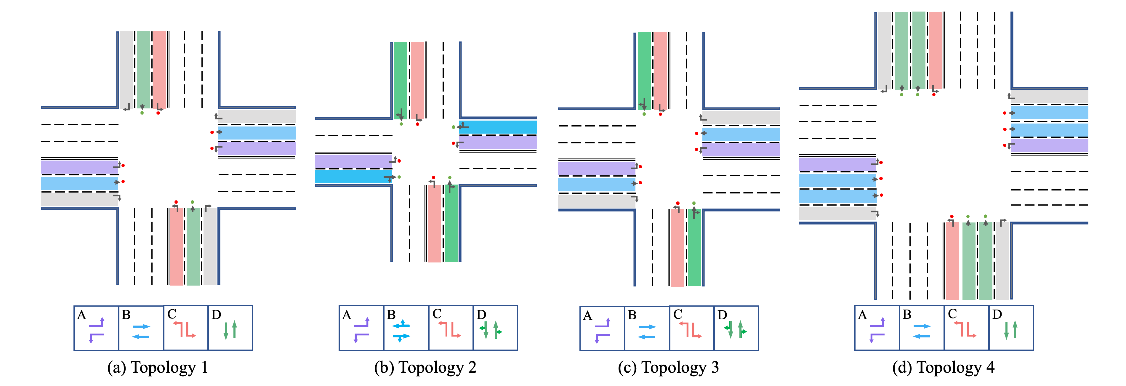
Figure 1: Illustration of four different intersection topologies with their available phases. Arrows represent traffic movements, and they can be organized into phases. Phase #D is actuated for the four intersections.

Advanced-XLight (Zhang et al. 2022) indirectly realized dynamic phase duration with an essential state representation: effective running vehicle number, which is the number of vehicles that can pass through the intersection within the action duration. The effective running vehicle number and traffic movement pressure enable an agent to learn whether to maintain or change the current signal phase, resulting in the duration of each phase becoming dynamic and flexible. The phase duration ($t_{phase}$) of Advanced-XLight can be $n\times t_{action}$ ($n\in\mathbb{N}^{+}$, $t_{action}$ is fixed, and $n$ is changeable) and Advanced-XLight can achieve better performance with smaller action duration ($t_{action}$). Therefore, the phase duration of Advanced-XLight is still not flexible enough because they heavily depend on the action duration of the control agent.

Several studies concentrated on cyclical signal control in the traditional TSC field (Le et al. 2015; Levin, Hu, and Odell 2020). However, very few studies concentrated on cyclical signal control (Liang et al. 2019) in the DRL-based TSC field due to the performance limitation and algorithm complexity.

3 Preliminary

Traffic network

A traffic network is usually described as a directed graph in which intersections and roads are represented by nodes and edges, respectively. Each road consists of several lanes, which are the basic units to support vehicle movement and determine the way each vehicle passes through an intersection, such as turning left, going straight, and turning right. An incoming lane is where vehicles enter the intersection, and an outgoing lane is where vehicles leave the intersection. We denote the set of incoming lanes and outgoing lanes of intersection $i$ as $\mathcal{L}_{i}^{in}$ and $\mathcal{L}_{i}^{out}$, respectively.

Traffic movement

Each traffic movement is defined as vehicles traveling across an intersection towards a certain direction, i.e., left, straight, and right. Some traffic movements can allow both to go straight and turn right. According to the traffic rules in some countries, vehicles that turn right can pass regardless of the signal but must stop at a red light. As shown in Figure 1, with different intersection topologies, each intersection has different types of traffic movements.

Signal phase

Each signal phase, denoted by $p$, is a set of permitted traffic movements, and $\mathcal{P}$ denotes the set of all the phases at each intersection. We use $\mathcal{L}_{p}^{in}$ to denote the participating incoming lanes of phase $p$. As shown in Figure 1, with different intersection topologies, each phase has different $\mathcal{L}_{p}^{in}$.

Action duration

The action duration is the time that each agent spends in each action, denoted by $t_{action}$. In our method, the action duration is not fixed and can dynamically change with different states.

Phase duration

The duration of each signal phase is the time that each phase spends within the green signal, denoted by $t_{phase}$. Similarly, in our method, the phase duration is not fixed and can dynamically change with different states.

State representation

The state representation of each intersection is lane-based, such as the number of vehicles and queue length on each incoming lane. We use $x_{i}(l),l\in\mathcal{L}^{in},i\in\mathbb{N}^{+}$ to represent the $i$-th characters on lane $l$.

The summary of notations is listed in Table 1.

Notation	Description
$\mathcal{L}^{in}_{i}$	set of incoming lanes of intersection $i$
$\mathcal{L}^{out}_{i}$	set of outgoing lanes of intersection $i$
$p$	phase which is a set of traffic movements
$\mathcal{P}_{i}$	available phases at intersection $i$
$\mathcal{L}_{p}^{in}$	participating incoming lanes of phase $p$
$x_{i}(l)$	the $i$-th characters of lane $l$
$t_{action}$	the duration of each action
$t_{phase}$	the duration of each phase
$\mathbb{N}^{+}$	a positive integer

Table 1: Summary of notations

Problem definition

In this paper, we consider multi-intersection TSC, in which each intersection is controlled by an RL agent. Agent $i$ views the environment as its observation $o_{i}^{t}$, takes action $a_{i}^{t}$ to control the signal phase of intersection $i$, and then obtain reward $r_{i}^{t}$. Each agent can learn a control policy by interacting with the environment. The goal of all the agents is to learn an optimal policy to maximize their cumulative reward, denoted as:

$$\sum_{t=1}^{T}\sum_{i=1}^{n}r_{i}^{t}$$ (1)

where $n$ is the number of RL agents and $T$ is the timestep. Each agent is also required to handle different intersection topologies for the convenience of deployment. To develop and evaluate our model, we consider four different intersection topologies (Figure 1) which are common in the real world.

4 Method

In this section, we first propose a two-stage TSC framework, i.e., DynamicLight. Then, we design a lite version of DynamicLight (i.e., DynamicLight-Lite) that only uses dozens of parameters to realize the dynamic phase duration. At last, we design a model with a cyclical phase structure that is suitable for deployment based on DynamicLight (i.e., DynamicLight-Cycle).

4.1 DynamicLight: Two-Stage Traffic Signal Control

As proposed above, we divide the TSC progress into two stages: phase control and duration control. The framework is illustrated in Figure 2.

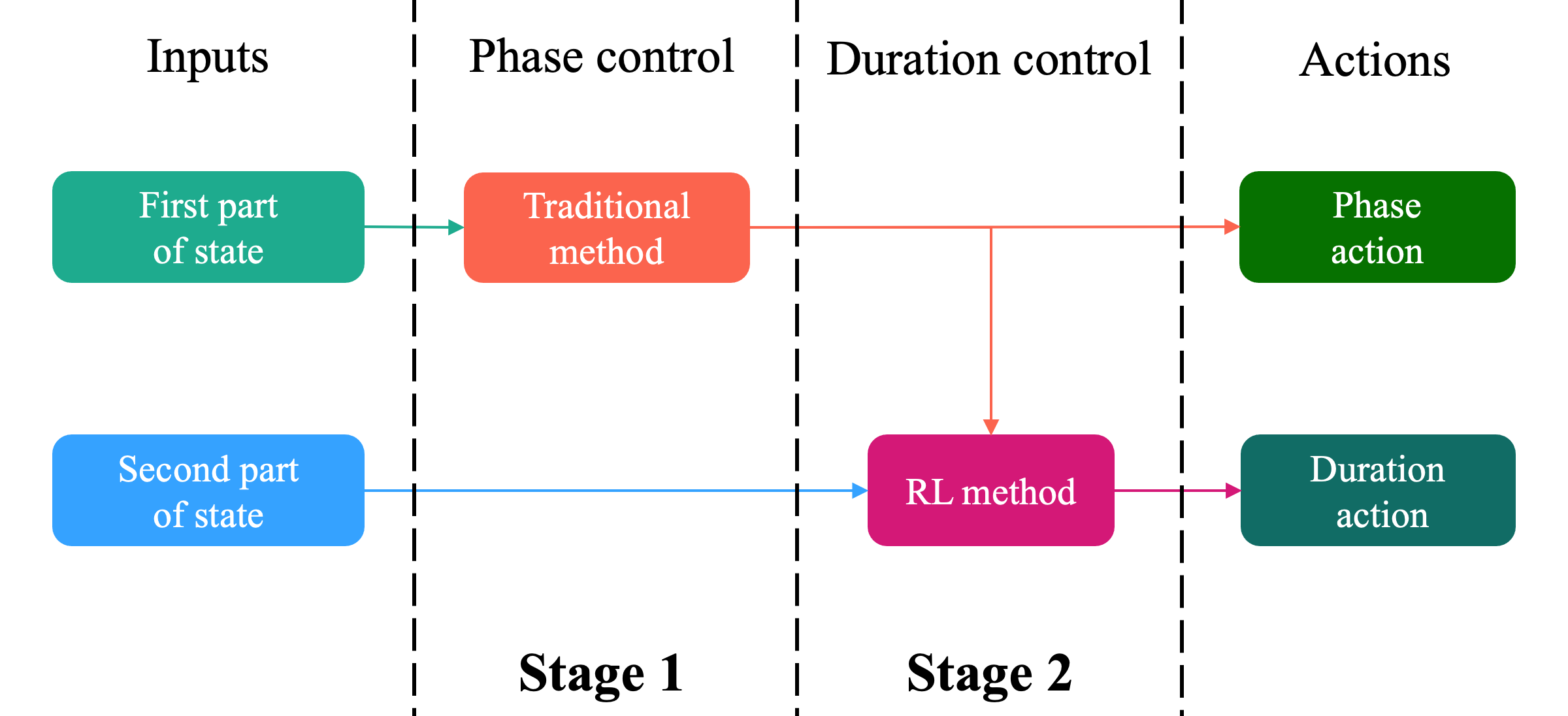
Figure 2: Overview framework of DynamicLight.

Phase control is used to choose the proper phase, and duration control is employed to determine the specific duration for the determined phase. According to the real-time traffic condition, a phase $\hat{p}$ is chosen to be actuated, and the corresponding phase duration $\hat{t_{phase}}$ is further determined. The phase control policy is realized with an optimization-based method, and duration control is realized by a deep Q-network (DQN). The DynamicLight is formally summarized in Algorithm 1.

Algorithm 1 DynamicLight

Parameters: Intersection number $n$; current actuated phase at intersection $i$: $\hat{p}_{i}$; duration of phase $\hat{p}_{i}$: $\hat{t}^{i}_{phase}$; current phase time at intersection $i$: $t^{i}$.

1:  Initialize $\hat{p}_{i}$, $\hat{t}^{i}_{phase}$, and $t^{i}$;

2:  for (time step) do

3:     for i=1:n do

4:        $t^{i}=t^{i}+1$;

5:        if $t^{i}=\hat{t}^{i}_{phase}$ then

6:           Determine the phase $\hat{p}_{i}$ for intersection $i$ with a phase control policy (such as M-QL);

7:           Determine the duration $\hat{t}_{phase}^{i}$ for phase $\hat{p}_{i}$ with a DQN;

8:           $t^{i}=0$;

9:        end if

10:     end for

11:  end for

In DynamicLight, the aim of phase control and duration control should be the same. The phase control uses an optimization-based method that formulates the TSC as an optimization problem. The optimization-based method can roughly optimize the target. For example, Max Pressure (MP) (Varaiya 2013) and Max Queue-Length (M-QL) (Zhang, Wu, and Deng 2022) can determine the phase but cannot determine a specific duration. We usually use a predefined action duration when using MP and M-QL, which makes the phase duration less flexible. In this case, the duration of each phase cannot exactly optimize the target.

In DynamicLight, we use a DQN to learn a policy to determine the duration. With the reward function of duration control being the same as the phase control, DynamicLight can determine a proper duration under each phase. The duration control can satisfactorily optimize the target of phase control. The phase control and duration control cooperate to optimize the same target.

Stage One: Phase Control

The following methods can be used as the phase control policy.

• M-QL (Zhang, Wu, and Deng 2022): selects the phase that has the maximum queue length. In this case, negative queue length should be used as the reward to update the DQN of duration control.

• Efficient-MP (Wu et al. 2021): selects the phase that has the maximum efficient pressure (Wu et al. 2021). In this case, negative absolute pressure should be used as the reward to update the DQN of duration control.

• Max State-Value (M-SV): selects the phase that has the maximum state value. The state value of each phase is calculated from the q-values of the duration action under the corresponding phase. In this case, both negative queue length and negative absolute pressure can be used as the reward to update the DQN of duration control.

DynamicLight has shown different performances with different phase control policies, and we conduct extensive experiments to evaluate them in the Experiments section. We finally use M-QL as the default phase control policy of DynamicLight.

Stage Two: Duration Control

We design a universal neural network that can apply to any intersection topology, such as AttendLight (Oroojlooy et al. 2020), for duration control. The network of duration control mainly consists of four modules: (1) lane feature embedding, (2) phase feature construction, (3) phase feature selection, and (4) duration score prediction. The network of duration control is illustrated in Figure 3.

Figure 3: Network design of duration control.

Lane feature embedding

The characteristics of each entering lane are first embedded from one-dimensional into a $d_{1}$-dimensional latent space via a layer of multi-layer perceptron (MLP):

$$h_{1}(l_{i})=\operatorname{Embed}(x_{i}(l))=\sigma(x_{i}(l)W_{e}+b_{e})$$ (2)

where $x_{i}(l),i=1,2,...,m,l\in\mathcal{L}^{in}$ is one of the characteristics of lane $l$, $m$ is the total number of characteristics, $W_{e}\in\mathbb{R}^{1\times d_{1}}$ and $b_{e}\in\mathbb{R}^{d_{1}}$ are weight matrix and bias vector to learn, $\sigma$ is the sigmoid function. In this paper, $d_{1}=4$. Next, the features belonging to one lane are concatenated to get the feature of each lane:

$$h_{2}(l)=\operatorname{Concatenate}(h_{1}(l_{1}),h_{1}(l_{2}),...,h_{1}(l_{m}))$$ (3)

Phase feature construction

The feature of each phase is constructed through feature fusion of the participating incoming lanes:

$$h_{3}(p)=\operatorname{Mean}(\operatorname{Attention}(h_{2}(l),...,h_{2}(k)),l,k\in\mathcal{L}_{p}$$ (4)

where $p$ is one phase, and $\mathcal{L}_{p}$ is the set of participating entering lanes of phase $p$. The feature fusion method is essential for building a universal model. In Appendix A.1, we discuss four feature fusion methods for phase feature construction and finally select multi-head self-attention as the default, and the head number selects 4 in our implementation.

Phase feature selection

The phase $\hat{p}$ is determined by M-QL control and we choose the feature of $\hat{p}$ for the duration score prediction:

$$f_{1}=h_{3}(\hat{p})$$ (5)

Duration score prediction

The phase features are further embedded via a MLP:

$$f_{2}=\operatorname{Embed}(f_{1})=\sigma(f_{1}W_{c}+b_{c})$$ (6)

where $W_{c}\in\mathbb{R}^{d_{2}\times c}$ and $b_{c}\in\mathbb{R}^{c}$ are weight matrix and bias vector to learn, $d_{2}=m\times d_{1}$,$\sigma$ is the ReLU function. In this paper, $d_{2}=16$. The dueling block (Wang et al. 2016) is followed to get the score of each duration action:

$$q=\operatorname{DuelingBlock}(f_{2})$$ (7)

Finally, we determine the duration action that has the maximum score, and the duration will be set according to a predefined duration action space. For example, if the duration action is $1$ with the action space as $\{10,15,20,25\}$, then the duration will be set to $15$.

The neural network of DynamicLight is carefully designed. In Appendix A.2, we also evaluate three different neural networks and select the best one as the default for DynamicLight.

DynamicLight Agent Design

For a DynamicLight agent, we introduce the state, action, and reward in detail.

• State. Two parts of the state are used in DynamicLight, one part for phase control and another part for duration control. Queue length on each entering lane is used for phase control, which is consistent with the M-QL policy. The number of vehicles under segmented roads is used for duration control. Specifically, we consider a segment of 400 meters from the intersection and split it into four chunks of 100 meters. Zero padding is used if the road is shorter than 400 meters.

• Action. Phase action: at time $t$, each agent first chooses a phase $\hat{p}$ as its phase action from phase action space $A$ based on the first part of the state, indicating the traffic signal should be set to phase $\hat{p}$. Duration action: each agent chooses a duration $\hat{t}_{phase}$ as the duration of $\hat{p}$ based on the second part of the state, indicating the traffic signal of phase $\hat{p}$ will last $\hat{t}_{phase}$. In this paper, the default phase action space is illustrated in Figure 1, and the duration action space is set as {10, 15, 20, 25, 30, 35, 40} (second).

• Reward. Negative intersection queue length is used as the reward. The reward for the agent that is controlling intersection $i$ is denoted by:

  $$r_{i}=-\sum q(l),l\in\mathcal{L}_{i}^{in}$$ (8)

  in which $q(l)$ is the queue length at lane $l$. This reward is corresponding to M-QL.

The DynamicLight agents are applied in a decentralized paradigm (Chen et al. 2020) to tackle the multi-agent TSC problem. Both parameters of the network and replay memory are shared among all the agents.

4.2 Model 2: DynamicLight-Lite

Based on a comprehensive understanding and analysis of the DQN of DynamicLight, we introduce DynamicLight-Lite. Compared to DynamicLight, the DQN of DynamicLight-Lite is different from the followings.

In the lane feature embedding module, DynamicLight-Lite embeds all the features of lane $l$ into a one-dimensional latent space with a MLP to get the feature of each lane:

$$h_{1}(l)=\operatorname{Embed}(x(l))=\sigma(x(l)W_{e}+b_{e})$$ (9)

where $x(l)\in\mathbb{R}^{4}$, $W_{e}\in\mathbb{R}^{4\times 1}$ and $b_{e}\in\mathbb{R}^{1}$ are weight matrix and bias vector to learn, $\sigma$ is the sigmoid function. The number of trainable parameters in this part is 5.

In the phase feature construction module, DynamicLight-Lite directly adds the features of $l,l\in\mathcal{L}_{p}$ to get the feature of phase $p$. There are no trainable parameters in this part. See Appendix A.1 for more details about this feature fusion method.

In the phase feature selection module, DynamicLight-Lite’s component is the same as DynamicLight. There are no trainable parameters either.

In the duration score prediction module, DynamicLight-Lite directly uses a MLP to get the score of each duration action:

$$q=\operatorname{Embed}(f)=\sigma(fW_{c}+b_{c})$$ (10)

where $f\in\mathbb{R}^{1}$ is the selected phase feature from the last module, $W_{c}\in\mathbb{R}^{1\times 7}$ and $b_{c}\in\mathbb{R}^{7}$ are weight matrix and bias vector to learn, $\sigma$ is the ReLU function. The trainable parameters in this part are 14.

Method	JiNan		HangZhou	Synthetic 1		Synthetic 2		Synthetic 3
	1	2	1	1	2	1	2	1	2
FixeTime	$585.76$	$411.63$	$611.65$	$527.74$	$787.22$	$400.87$	$671.86$	$252.99$	$261.58$
M-QL	$288.84$	$248.36$	$300.54$	$188.09$	$234.80$	$173.78$	$204.79$	$164.09$	$173.03$
Efficient-MP	$286.37$	$247.75$	$299.73$	$194.09$	$241.71$	$176.29$	$207.04$	$165.52$	$174.65$
CoLight	$283.14$	$257.44$	$311.54$	$208.63$	$273.69$	$186.17$	$227.86$	$171.33$	$180.69$
AttendLight	$297.50$	$255.86$	$304.84$	$200.38$	$254.79$	$176.54$	$211.72$	$169.41$	$179.11$
Efficient-MPLight	$279.42$	$250.59$	$301.26$	$195.58$	$240.08$	$177.17$	$204.60$	$165.87$	$176.10$
AttentionLight	$270.14$	$247.16$	$300.22$	${189.14}$	${223.64}$	${173.49}$	${200.54}$	$164.09$	$172.77$
Advanced-CoLight	${259.31}$	${240.61}$	$\mathbf{285.33}$	$203.25$	$318.61$	$176.70$	$215.31$	${161.66}$	${171.19}$
DynamicLight	$\mathbf{254.69}$	$\mathbf{237.53}$	$286.10$	$\mathbf{178.40}$	$\mathbf{209.15}$	$\mathbf{162.52}$	$\mathbf{188.52}$	$\mathbf{154.90}$	$\mathbf{165.70}$
DynamicLight-Lite	$265.23$	$245.40$	$297.39$	$181.48$	$215.19$	$164.58$	$197.43$	$161.37$	$173.05$
DynamicLight-Cycle	$282.93$	$261.14$	$324.65$	$238.68$	$248.85$	$192.12$	$217.26$	$179.49$	$185.09$

Table 2: Overall performance comparison. For adjusted average travel time (in seconds), the smaller the better.

In summary, we use MLP twice, the first MLP contains 5 trainable parameters and the last MLP contains 14 trainable parameters. Other modules do not contain trainable parameters, and the total trainable parameters of DynamicLight-Lite is 19. DynamicLight-Lite only uses less than two dozen of parameters and has significantly fewer parameters than other RL models for TSC. For example, FRAP (Zheng et al. 2019a) contains about $1369$ parameters, CoLight contains about $18756$ parameters, AttentionLight (Zhang, Wu, and Deng 2022) contains about $3101$ parameters, and DynamicLight contains about $3936$ parameters.

4.3 Model 3: DynamicLight-Cycle

In a real-world deployment, the phase is usually required in a fixed cyclical order due to its simple and stable industrial implementation. Cyclical signal control is described as a policy that actuates the phase with a fixed cyclical order, and FixedTime (Koonce and Rodegerdts 2008) is a typical cyclical signal control method. Due to the property of DynamicLight that it determines the phase and duration at different stages, we can replace the M-QL with the cyclical signal control policy to realize the cyclical phase structure. We refer to the DynamicLight with cyclical signal control for phase determination as DynamicLight-Cycle. Overall, DynamicLight-Cycle uses cyclical signal control to determine the phase and uses a DQN that is the same as DynamicLight to determine the corresponding duration.

DynamicLight-Cycle can be realized in the following two ways: (1) directly train it on the target dataset; (2) transfer the DQN of duration control from properly pre-trained DynamicLight. DynamicLight-Cycle has better performance with transfer from DynamicLight than directly training it, and we finally construct DynamicLight-Cycle by transferring it from a pre-trained DynamicLight.

5 Experiments

5.1 Settings

We conduct comprehensive experiments on CityFlow (Zhang et al. 2019), which is open-source and supports large-scale TSC. Each green signal is followed by a five-second yellow signal to prepare for the signal phase transition. To fully evaluate DynamicLight, DynamicLight-Lite, and DynamicLight-Cycle, we use two groups (JiNan and HangZhou) of real-world datasets (Zheng et al. 2019a; Wei et al. 2019b) and three groups of synthetic datasets to conduct experiments. There are totally nine traffic flow datasets: two from JiNan; one from HangZhou; two from Synthetic 1; two from Synthetic 2; and two from Synthetic 3. These datasets contain four different intersection topologies, as shown in Figure 1: JiNan and HangZhou contain topology 1; Synthetic 1 contains topology 2; Synthetic 2 contains topology 3; and Synthetic 3 contains topology 4.

With the problem of average travel time and throughput (more detailed analysis in Appendix B), we propose adjusted average travel time (AATT) that extends the time of each testing episode to enable all the vehicles can pass through the traffic network. The AATT can evaluate the model performance with the same throughput in a fair way and it is used as the evaluation metric for methods comparison.

We compare our proposed methods with: FixedTime (Koonce and Rodegerdts 2008), uses fixed cycle length with a predefined phase split among all the phases; M-QL (Zhang, Wu, and Deng 2022), actuates the phase that has the maximum queue length; Efficient-MP (Wu et al. 2021), actuates the phase that has the maximum efficient pressure; CoLight (Wei et al. 2019b), uses graph attention nueral network (Velickovic et al. 2017) to realize intersection coorperation; AttendLight (Oroojlooy et al. 2020), uses attention mechanism (Vaswani et al. 2017) to construct phase feature and predict phase transition probability; Efficient-MPLight (Wu et al. 2021), uses FRAP as the neural network and introduces efficient pressure into state design; AttentionLight (Zhang, Wu, and Deng 2022), uses attention mechanism (Vaswani et al. 2017) to model phase competition; and Advanced-CoLight (Zhang et al. 2022), uses CoLight as the base neural network and introduces effective running vehicle and efficient pressure as state representations. More details on datasets and training details are provided in Appendix C.

5.2 Overall Performance

Table 2 demonstrates the overall performance under multiple real-world and synthetic datasets concerning the AATT. DynamicLight outperforms all other existing methods using both real-world and synthetic datasets. DynamicLight achieves a new state-of-the-art performance for TSC. In addition, with only 19 trainable parameters, DynamicLight-Lite still outperforms most other methods except Advanced-CoLight. The performances of DynamicLight and DynamicLight-Lite indicate that the two-stage TSC framework is powerful and efficient.

Dynamic phase duration can significantly improve the TSC efficiency. Under the same phase control policy, DynamicLight and DynamicLight-Lite significantly outperform M-QL with a dynamic phase duration, and DynamicLight-Cycle significantly outperforms FixedTime with a dynamic phase duration. In addition, DynamicLight-Cycle demonstrates high performance and outperforms CoLight and AttendLight in some datasets. Duration control is as essential as phase control for improving transportation efficiency.

5.3 Different Phase Control Methods

Extensive experiments are conducted on real-world and synthetic datasets to evaluate how DynamicLight performs with the following four phase control methods:

• Method 1. M-QL is used to determine the phase and the reward of DynamicLight is set as negative queue length. It is the default phase control policy for DynamicLight in this article.

• Method 2. Efficient-MP is used to determine the phase and the reward is set as negative absolute pressure.

• Method 3. M-SV is used to determine the phase and the reward is set as negative queue length.

• Method 4. M-SV is used to determine the phase and the reward is set as negative absolute pressure.

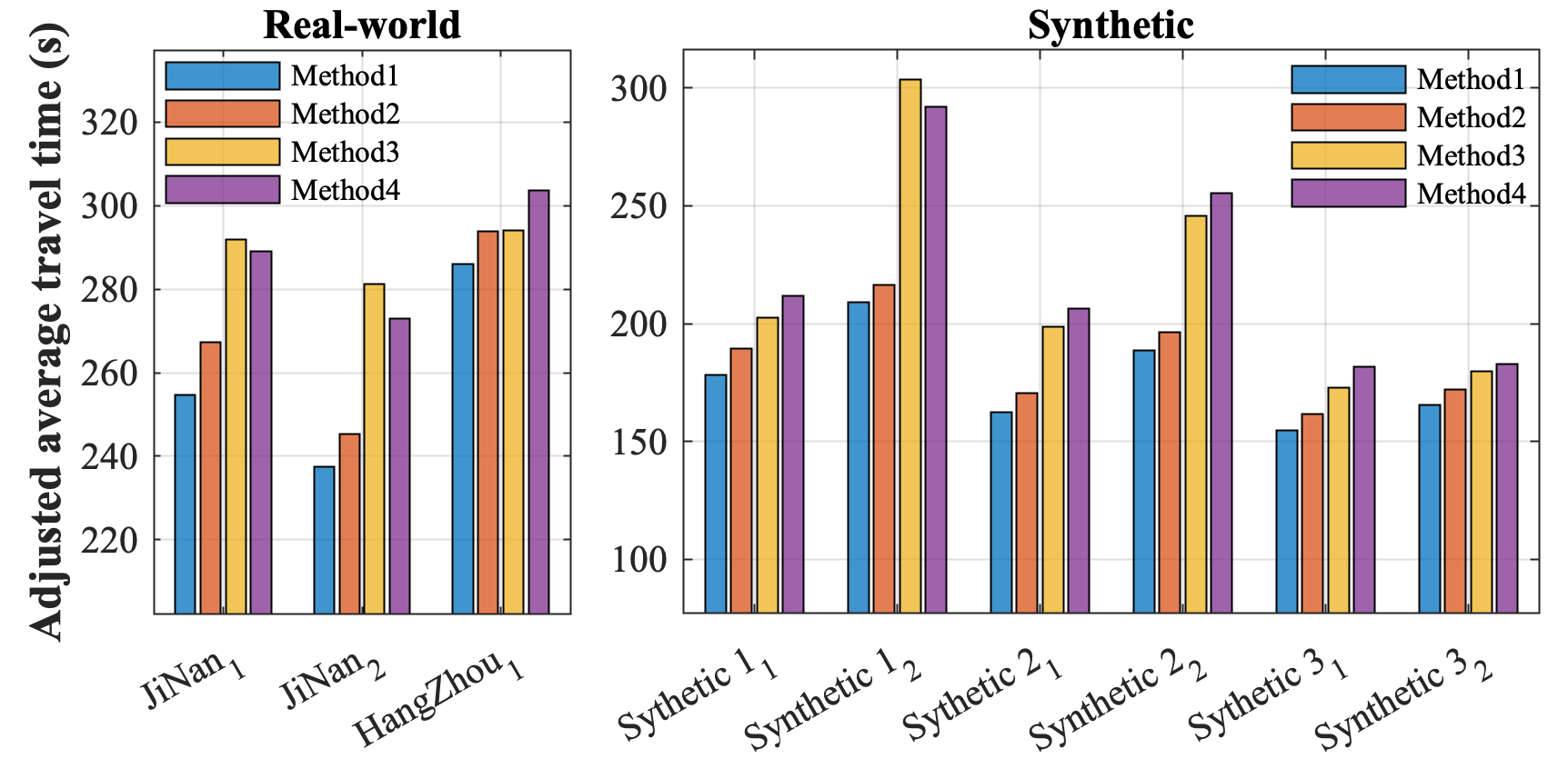
Figure 4: The performance of DynamicLight with different phase control policies.

Specifically, the DQN of Method 1 and Method 2 uses the default network as described in Figure 3, while the DQN of Method 3 and Method 4 uses a similar but different one (see Appendix A.2 for more details). Figure 4 demonstrates the performance of DynamicLight with different phase control policies. DynamicLight has better performance under M-QL than Efficient-MP and M-SV. In addition, under Efficient-MP, DynamicLight also demonstrates high performance among all the datasets, indicating that the framework of DynamicLight is powerful.

5.4 Model Generalization

The generalization of DynamicLight and DynamicLight-Lite are studied with training on each dataset and transferring to other datasets. We use the AATT ratio to evaluate the generalization, denoted as $t_{transfer}/t_{train}$, where $t_{train}$ is the AATT of direct training and $t_{transfer}$ is the AATT of transfer. The smaller of $t_{transfer}/t_{train}$, the better of the model generalization.

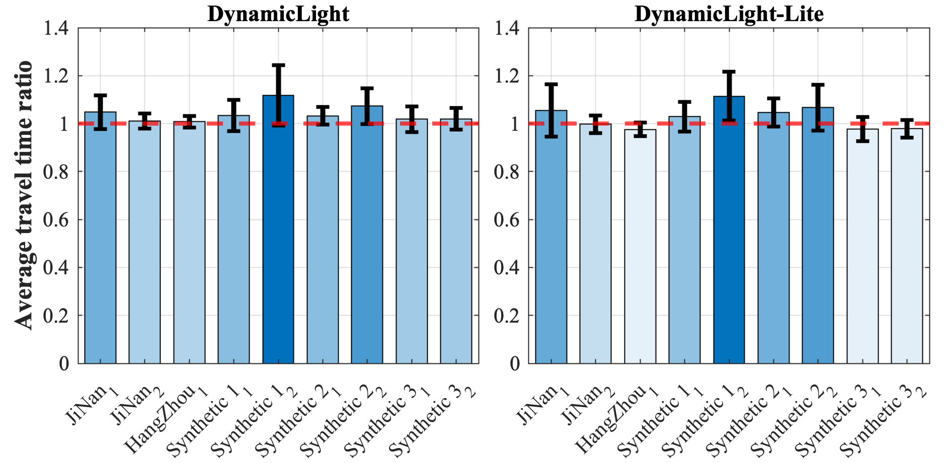
Figure 5: The AATT of transfer divided by the AATT of direct training. The error bars represent 95% confidence interval for the AATT ratio.

Figure 5 demonstrates the AATT ratio of DynamicLight and DynamicLight-Lite over all the datasets. DynamicLight and DynamicLight-Lite demonstrate pretty good generalization ability on intersections with different topologies. The generalization also ensures the reliability of DynamicLight-Cycle because it requires the pre-trained network of DynamicLight. With few trainable parameters, DynamicLight-Lite has a slightly better AATT ratio than DynamicLight, indicating that our two-stage framework is reliable.

5.5 Model Deployment

DynamicLight, DynamicLight-Lite, and DynamicLight-Cycle fully consider deployment issues. When the phase sequence is allowed in an arbitrary order, DynamicLight and DynamicLight-Lite show high performance and generalization ability. Especially, DynamicLight-Lite contains 19 parameters and has few hardware requirements. Furthermore, DynamicLight-Lite has far fewer parameters than other DRL models, such as CoLight and FRAP, so it is more reliable for deployment.

If the phase sequence is required in cyclical order, DynamicLight-Cycle supports cyclical phase structure and demonstrates pretty high performance. DynamicLight-Cycle significantly outperforms FixedTime (Koonce and Rodegerdts 2008) which is wildly used in most cities currently, as it can yield significant transportation efficiency improvement. The demonstrated performance of DynamicLight-Lite and DynamicLight-Cycle indicates they are promising solutions for real-world traffic signal control.

Besides the high performance, DynamicLight can adapt to different types of intersections. We can train it on the most common intersection but deploy it at other intersections directly, reducing the workload of model training and deployment.

6 Conclusion

In this paper, we reexamined the traffic signal control problem and proposed a two-stage traffic signal control framework, which first determined the phase and then the duration. An optimization-based method was used to implement the phase control, while DRL was used to learn the duration control. Based on the novel framework, we proposed three models: DynamicLight, DynamicLight-Lite, and DynamicLight-Cycle. Comprehensive experiments using real-world datasets demonstrated that DynamicLight outperformed all the existing methods, and DynamicLight-Lite showed better performance than most existing methods. With carefully pre-trained DynamicLight, the phase control was replaced with a cyclical signal control policy that can also demonstrate high performance. Our proposed DynamicLight, DynamicLight-Lite, and DynamicLight-Cycle not only demonstrated high performance but also ensured flexibility for deployment.

In future research, we will try to find an effective framework that allows DynamicLight to cooperate with each other to control the traffic signal of the entire traffic network.

Appendix A Extended Model Study

Appendix A provides extensive experiments of DynamicLight under different configurations. When studying the influence of one key element, the configuration of other elements is set the same as that in the body of the paper.

A.1 Feature Fusion Methods

Four methods can be used for feature fusion, they are configured as follows:

• Method 1. The features of the participating incoming lanes are modeled with multi-head self-attention (Vaswani et al. 2017) and then averaged to get the features of the corresponding phase. This approach is used by DynamicLight.

• Method 2. The features of the participating incoming lanes are first averaged; then the attention mechanism is used to model the averaged features and original features. This method is adopted from the AttendLight (Oroojlooy et al. 2020).

• Method 3. The features of the participating incoming lanes are first concatenated and then embedded into the same dimension.

• Method 4. The features of the participating incoming lanes are directly added. It is the same as that in FRAP (Zheng et al. 2019a) and is used by DynamicLight-Lite.

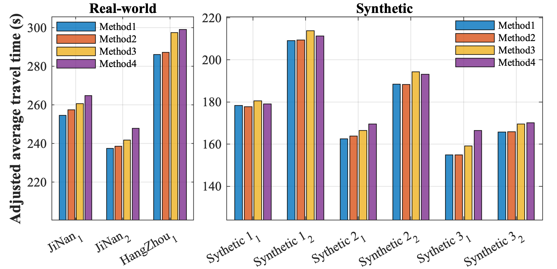
Figure 6: The performance of DynamicLight under different feature fusion methods.

Figure 6 demonstrates the performance of DynamicLight under different feature fusion methods. The feature fusion methods significantly influence the performance of DynamicLight, but they are all reliable methods for feature fusion.

A.2 Neural Network Study

We evaluate how DynamicLight performs with three different neural networks. Figure 7 illustrates the design of the three neural networks. Compared to Network 2 and Network 3, Network 1 only outputs the q-values of the pre-determined phase $\hat{p}$, while Network 2 and Network 3 output the q-values of all the phases. Compared to Network 2, Network 3 uses self-attention to model the phase correlation like AttentionLight (Zhang, Wu, and Deng 2022), while Network 2 ignores it.

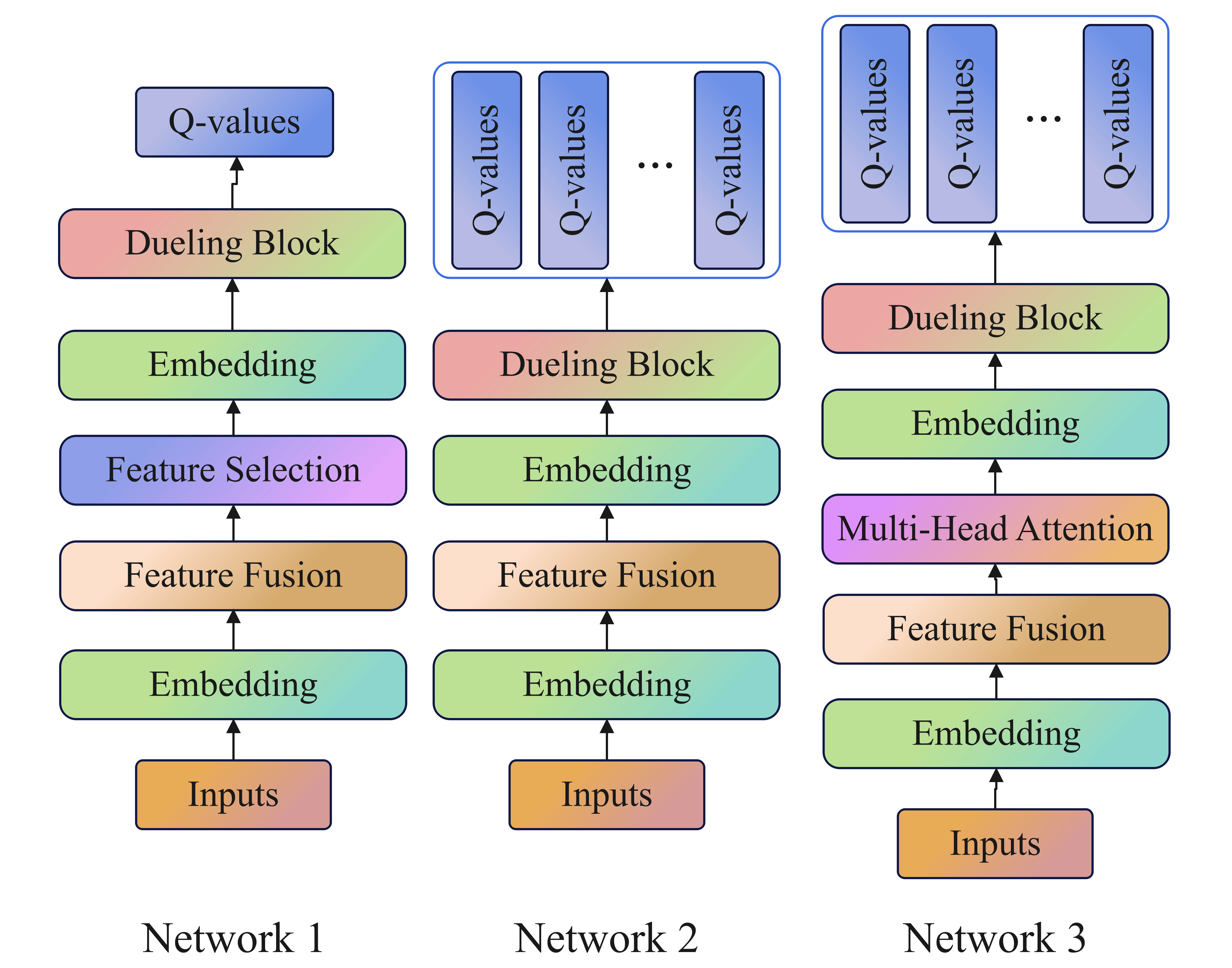
Figure 7: Illustration of three neural networks.

Figure 8 reports the performance of DynamicLight under the three neural networks. The choice of the neural network significantly influences the model performance, and DynamicLight yields the best performance under Network 1 among all the datasets. We finally choose Network 1 as the default neural network for DynamicLight.

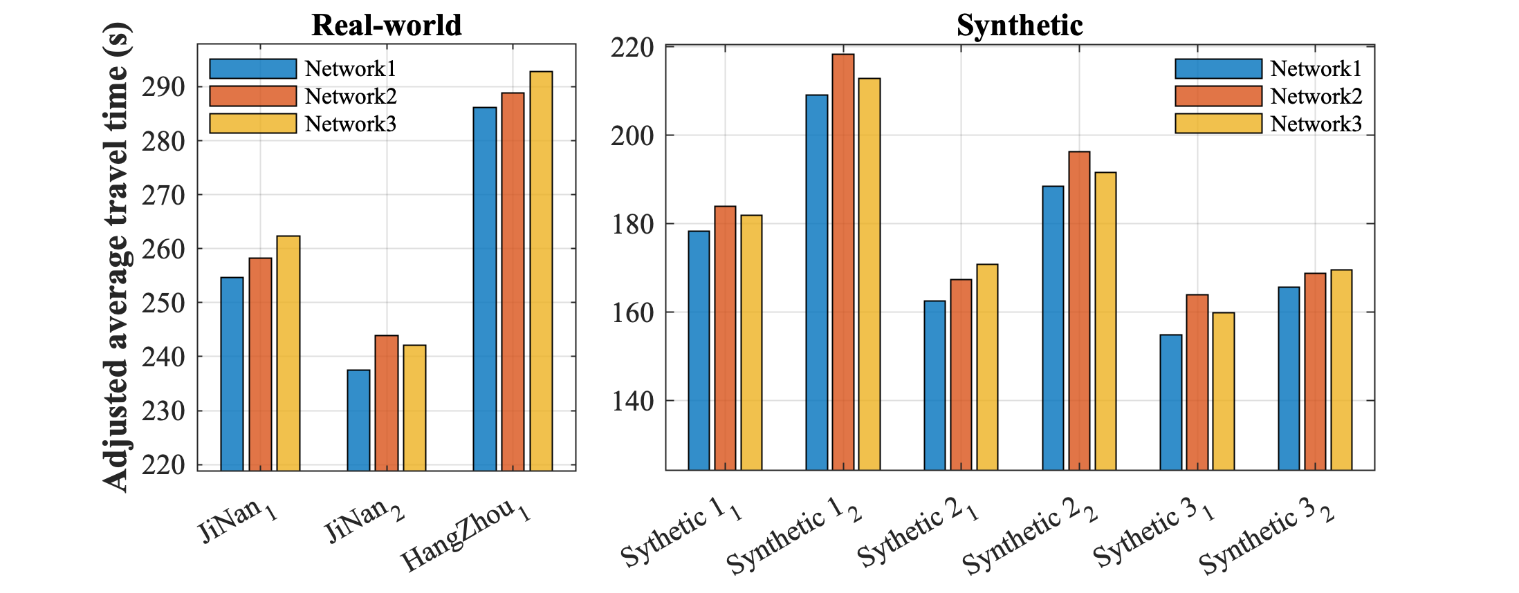
Figure 8: The performance of DynamicLight under different neural networks.

Importantly, when using Max State-Value (M-SV) to determine the phase, DynamicLight cannot converge with Network 1 and Network 2 but it can get a high performance under Network 3. Therefore, the neural network structure should adopt Network 3 if M-SV is used as the phase control policy.

Appendix B Problems of Current Evaluation Metrics

Each vehicle travels across the traffic network with a pre-defined start time and route. The start time determines when the vehicle starts entering the traffic network, and the routes usually have different lengths which heavily influence the travel time of each vehicle apart from the waiting time at each intersection. For example, as shown in Figure 9, Route 1, Route 2, and Route 3 are 500 meters, 400 meters, and 300 meters respectively. If a vehicle moves with a maximum speed (10m/s) on each route, the minimal travel time at Route 1, Route 2, and Route 3 are 50 seconds, 40 seconds, and 30 seconds. The difference in routes significantly affects the travel time of each vehicle. When calculating the average travel time, if the vehicles that pass through are not the same, we cannot determine which method is better than another with a smaller average travel time.

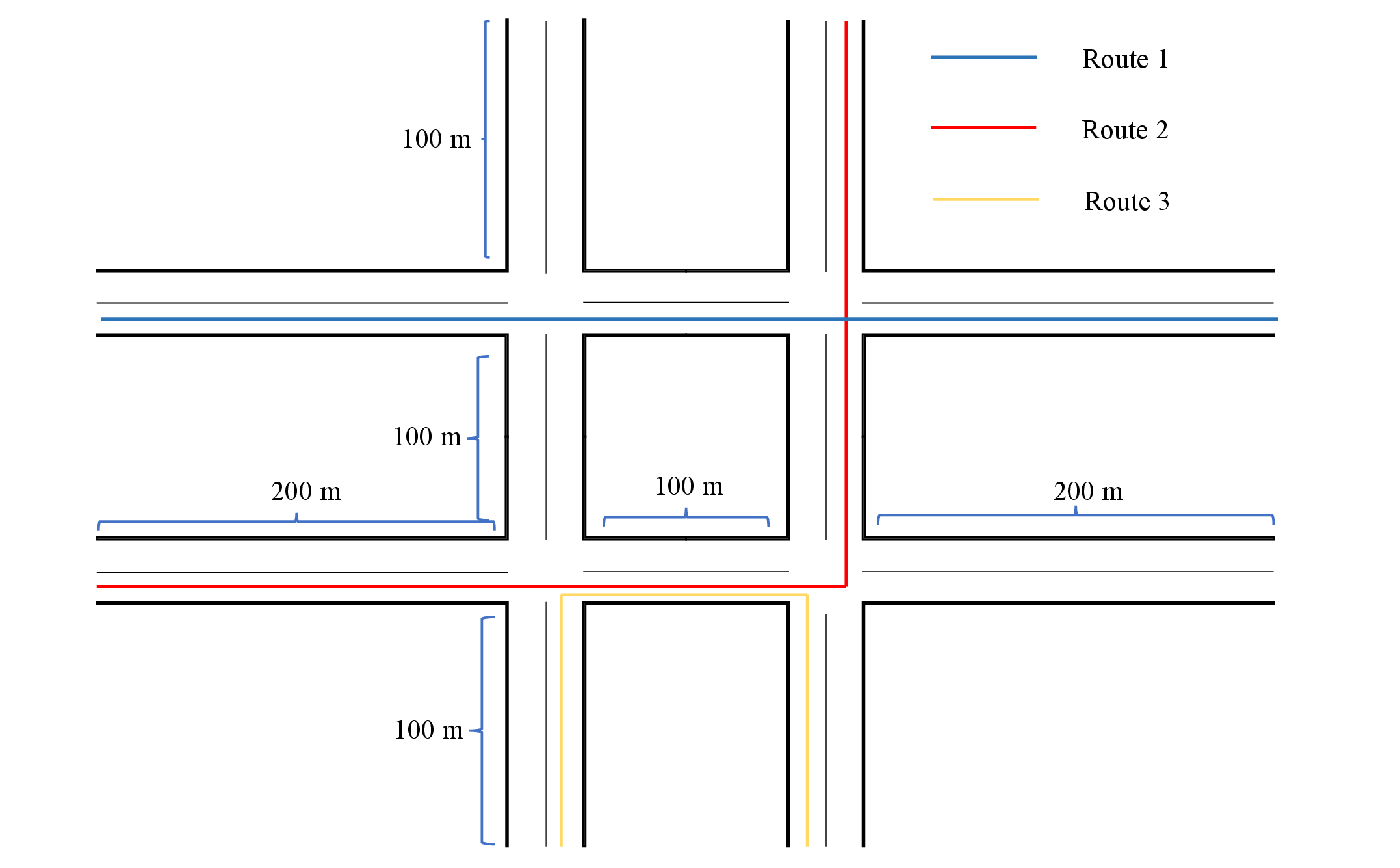
Figure 9: An example of a traffic network with three pre-defined routes.

Besides the influence of routes and control methods, the throughput is also influenced by the vehicle travel pattern. The time of each training episode is 3600 seconds, but if the time of each testing episode is also 3600 seconds, the vehicles that start entering at the end period of the simulation cannot pass through. We use $t_{1},t_{1}<3600$ to denote a critical time, that any vehicle cannot pass through if it starts entering the traffic network after $t_{1}$. With different control methods, the $t_{1}$ are different from each other. When using throughput to compare two methods, the difference in throughput is the number of vehicles that start entering the traffic network between two different $t_{1}$. If there are no vehicles that start entering the traffic network between two $t_{1}$, the throughput of the two methods are the same and we cannot compare the two methods. Therefore, the throughput and average travel time cannot evaluate model performance fairly.

Appendix C Numerical Experiments Details

C.1 Details of Real-world Datasets and Synthetic Datasets

Each traffic dataset consists of two parts: the traffic network dataset and the traffic flow dataset. The traffic network dataset describes the lanes, roads, intersections, and signal phases. The traffic flow dataset describes how vehicles travel across the network, denoted as $(t,u)$, in which $t$ is the time when the vehicle enters the traffic network, and $u$ is the pre-defined route from its original location to its destination. After the traffic data is fed into the simulator, each vehicle moves according to the pre-defined route $u$ at time $t$.

We use five groups of datasets consisting of nine datasets, two from JiNan, one from HangZhou, six are synthetic. The intersections of these datasets contain four different topologies. These datasets are described as follows:

• JiNan datasets: The road network has 12 ($3\times 4$) intersections. Each intersection has the same topology as that illustrated in Figure 1 (a) (in the body of the paper, the same goes for the following), which connects two 400-meter(East-West) long road segments and two 800-meter(South-North) long road segments. There are two traffic flow datasets under this traffic network.

• HangZhou dataset: The road network has 16 ($4\times 4$) intersections. Each intersection has the same topology as illustrated in Figure 1 (a), which connects two 800-meter(East-West) long road segments and two 600-meter(South-North) long road segments. There are one traffic flow dataset under this traffic network.

• Synthetic1 datasets: The road network has 12 ($3\times 4$) intersections. Each intersection has the same topology as illustrated in Figure 1 (b), which connects four 400-meter-long road segments. There are two traffic flow datasets under this traffic network.

• Synthetic2 datasets: The road network has 12 ($3\times 4$) intersections. Each intersection has the same topology as illustrated in Figure 1 (c), which connects four 400-meter-long road segments. There are two traffic flow datasets under this traffic network.

• Synthetic3 datasets: The road network has 12 ($3\times 4$) intersections. Each intersection has the same topology as illustrated in Figure 1 (d), which connects four 400-meter-long road segments. There are two traffic flow datasets under this traffic network.

The synthetic traffic flow datasets are randomly generated based on the traffic network datasets which are hand-crafted. The turn ratio of the synthetic traffic flow datasets is as follows: $10\%$ turning left, $60\%$ going straight, and $30\%$ turning right.

C.2 Details of the RL training

For a fair comparison, the action duration of all the baseline methods is set as 15-second. In addition, all the RL methods (including our proposed methods) use the same hyper-parameters. The learning rate is $0.001$, the early stopping patience is $10$, the batch size is $20$, the maximum memory is $12000$, the sample size for the update is $3000$, the $\gamma$ for update q-values is $0.8$, the training and testing epoch number is 80. We would like to emphasize that we have not performed any structured hyper-parameters tuning of DynamicLight, and the reported performance in this article might not be the best.

Each training episode is a 60-minute simulation, and the time of each testing episode is longer than 60 minutes to ensure that all the vehicles can pass through the traffic network. We obtain one result as the average of the last ten episodes of testing, and each reported result is the average of three independent experiments.

To ensure all the vehicles can pass through, we use the time under FixedTime (Koonce and Rodegerdts 2008) as the baseline time. For other methods, the time can be smaller than that under FixedTime. For simplicity, we set the testing time under FixedTime for all the methods. However, CoLight-based methods(CoLight and Advanced-CoLight) have limited capacity to make sure all the vehicles pass through although they have demonstrated high performance under average travel time. This may be because CoLight-based methods encounter fewer scenarios in the training progress due to the different episode times of training and testing. As a result, the time of each testing episode of CoLight-based methods should be much longer than the baseline time.

References

- Chen et al. (2020) Chen, C.; Wei, H.; Xu, N.; Zheng, G.; Yang, M.; Xiong, Y.; Xu, K.; and Li, Z. 2020. Toward a thousand lights: Decentralized deep reinforcement learning for large-scale traffic signal control. In Proceedings of the AAAI Conference on Artificial Intelligence, volume 34, 3414–3421.
- Chenguang, Xiaorong, and Gang (2021) Chenguang, Z.; Xiaorong, H.; and Gang, W. 2021. PRGLight: A novel traffic light control framework with Pressure-based-Reinforcement Learning and Graph Neural Network. In IJCAI 2021 Reinforcement Learning for Intelligent Transportation Systems (RL4ITS) Workshop.
- Finn, Abbeel, and Levine (2017) Finn, C.; Abbeel, P.; and Levine, S. 2017. Model-agnostic meta-learning for fast adaptation of deep networks. In International conference on machine learning, 1126–1135. PMLR.
- Koonce and Rodegerdts (2008) Koonce, P.; and Rodegerdts, L. 2008. Traffic signal timing manual. Technical report, United States. Federal Highway Administration.
- Kulkarni et al. (2016) Kulkarni, T. D.; Narasimhan, K.; Saeedi, A.; and Tenenbaum, J. 2016. Hierarchical deep reinforcement learning: Integrating temporal abstraction and intrinsic motivation. Advances in neural information processing systems, 29.
- Le et al. (2015) Le, T.; Kovács, P.; Walton, N.; Vu, H. L.; Andrew, L. L.; and Hoogendoorn, S. S. 2015. Decentralized signal control for urban road networks. Transportation Research Part C: Emerging Technologies, 58: 431–450.
- Levin, Hu, and Odell (2020) Levin, M. W.; Hu, J.; and Odell, M. 2020. Max-pressure signal control with cyclical phase structure. Transportation Research Part C: Emerging Technologies, 120: 102828.
- Liang et al. (2019) Liang, X.; Du, X.; Wang, G.; and Han, Z. 2019. A deep reinforcement learning network for traffic light cycle control. IEEE Transactions on Vehicular Technology, 68(2): 1243–1253.
- Lowrie (1990) Lowrie, P. 1990. Scats: A traffic responsive method of controlling urban traffic. Sales information brochure published by Roads & Traffic Authority, Sydney, Australia.
- Ma et al. (2017) Ma, W.; Liu, Y.; Zhao, J.; and Wu, N. 2017. Increasing the capacity of signalized intersections with left-turn waiting areas. Transportation Research Part A: Policy and Practice, 105: 181–196.
- Mnih et al. (2013) Mnih, V.; Kavukcuoglu, K.; Silver, D.; Graves, A.; Antonoglou, I.; Wierstra, D.; and Riedmiller, M. 2013. Playing atari with deep reinforcement learning. arXiv preprint arXiv:1312.5602.
- Oroojlooy et al. (2020) Oroojlooy, A.; Nazari, M.; Hajinezhad, D.; and Silva, J. 2020. Attendlight: Universal attention-based reinforcement learning model for traffic signal control. Advances in Neural Information Processing Systems, 33: 4079–4090.
- Sutton and Barto (2018) Sutton, R. S.; and Barto, A. G. 2018. Reinforcement learning: An introduction. MIT press.
- Varaiya (2013) Varaiya, P. 2013. Max pressure control of a network of signalized intersections. Transportation Research Part C: Emerging Technologies, 36: 177–195.
- Vaswani et al. (2017) Vaswani, A.; Shazeer, N.; Parmar, N.; Uszkoreit, J.; Jones, L.; Gomez, A. N.; Kaiser, Ł.; and Polosukhin, I. 2017. Attention is all you need. Advances in neural information processing systems, 30.
- Velickovic et al. (2017) Velickovic, P.; Cucurull, G.; Casanova, A.; Romero, A.; Lio, P.; and Bengio, Y. 2017. Graph attention networks. stat, 1050: 20.
- Wang et al. (2016) Wang, Z.; Schaul, T.; Hessel, M.; Hasselt, H.; Lanctot, M.; and Freitas, N. 2016. Dueling network architectures for deep reinforcement learning. In International conference on machine learning, 1995–2003. PMLR.
- Wei et al. (2019a) Wei, H.; Chen, C.; Zheng, G.; Wu, K.; Gayah, V.; Xu, K.; and Li, Z. 2019a. Presslight: Learning max pressure control to coordinate traffic signals in arterial network. In Proceedings of the 25th ACM SIGKDD International Conference on Knowledge Discovery & Data Mining, 1290–1298.
- Wei et al. (2019b) Wei, H.; Xu, N.; Zhang, H.; Zheng, G.; Zang, X.; Chen, C.; Zhang, W.; Zhu, Y.; Xu, K.; and Li, Z. 2019b. Colight: Learning network-level cooperation for traffic signal control. In Proceedings of the 28th ACM International Conference on Information and Knowledge Management, 1913–1922.
- Wei et al. (2018) Wei, H.; Zheng, G.; Yao, H.; and Li, Z. 2018. Intellilight: A reinforcement learning approach for intelligent traffic light control. In Proceedings of the 24th ACM SIGKDD International Conference on Knowledge Discovery & Data Mining, 2496–2505.
- Wu et al. (2021) Wu, Q.; Zhang, L.; Shen, J.; Lü, L.; Du, B.; and Wu, J. 2021. Efficient Pressure: Improving efficiency for signalized intersections. arXiv:2112.02336.
- Xu et al. (2021) Xu, B.; Wang, Y.; Wang, Z.; Jia, H.; and Lu, Z. 2021. Hierarchically and Cooperatively Learning Traffic Signal Control. In Proceedings of the AAAI Conference on Artificial Intelligence, volume 35, 669–677.
- Zang et al. (2020) Zang, X.; Yao, H.; Zheng, G.; Xu, N.; Xu, K.; and Li, Z. 2020. Metalight: Value-based meta-reinforcement learning for traffic signal control. In Proceedings of the AAAI Conference on Artificial Intelligence, volume 34, 1153–1160.
- Zhang et al. (2019) Zhang, H.; Feng, S.; Liu, C.; Ding, Y.; Zhu, Y.; Zhou, Z.; Zhang, W.; Yu, Y.; Jin, H.; and Li, Z. 2019. Cityflow: A multi-agent reinforcement learning environment for large scale city traffic scenario. In The World Wide Web Conference, 3620–3624.
- Zhang, Wu, and Deng (2022) Zhang, L.; Wu, Q.; and Deng, J. 2022. AttentionLight: Rethinking queue length and attention mechanism for traffic signal control. arXiv:2201.00006.
- Zhang et al. (2022) Zhang, L.; Wu, Q.; Shen, J.; Lü, L.; Du, B.; and Wu, J. 2022. Expression might be enough: representing pressure and demand for reinforcement learning based traffic signal control. In Proceedings of the 39th International Conference on Machine Learning, volume 162 of Proceedings of Machine Learning Research, 26645–26654. PMLR.
- Zheng et al. (2019a) Zheng, G.; Xiong, Y.; Zang, X.; Feng, J.; Wei, H.; Zhang, H.; Li, Y.; Xu, K.; and Li, Z. 2019a. Learning phase competition for traffic signal control. In Proceedings of the 28th ACM International Conference on Information and Knowledge Management, 1963–1972.
- Zheng et al. (2019b) Zheng, G.; Zang, X.; Xu, N.; Wei, H.; Yu, Z.; Gayah, V.; Xu, K.; and Li, Z. 2019b. Diagnosing reinforcement learning for traffic signal control. arXiv preprint arXiv:1905.04716.