Achieving one-dimensionality with attractive fermions

Abstract

In this article we discuss the accuracy of effective one-dimensional theories used to describe the behavior of ultracold atomic ensembles confined in quantum wires by a harmonic trap. We derive within a fully many-body approach the effective Hamiltonian describing this class of systems and we calculate the beyond-mean field corrections to the energy of the ground state arising from virtual transitions towards excited state of the confining potential. We find that, due to the Pauli principle, effective finite-range corrections are one of magnitude larger than effective three-body interactions. By comparing to exact solutions of the purely 1D problem, we conclude that a 1D effective theory provides a good description of the ground state of the system for a rather large range of interaction parameters.

I Introduction

Among quantum technologies, quantum simulation aims at finding the properties of complex Hamiltonians by engineering experimental systems whose dynamics can be described as precisely as possible by the problem under study Bloch et al. (2008); Georgescu et al. (2014). Within this program, ultracold atoms have been used in the past decade to solve Bertsch’s many-body X-challenge on the structure of strongly correlated quantum patter Zwerger (2012), or to emulate lattice models Browaeys and Lahaye (2020).

In this context the control of the experimental parameters is paramount to the success of the quantum simulation program and in this article we discuss the feasibility of the simulation of low dimensional systems using ultracold systems. Experimentally, low-dimensionality can be achieved by strongly compressing particles along one or two dimensions. When the energy of the particles is lower than the distance between the ground state and the first excited state of the trapping potential, the dynamics is frozen along these directions and we can consider the system as being kinematically 1D or 2D.

In this article, we focus on one-dimensional fermionic systems. These systems are accessible experimentally using cold atoms and have been used in recent years to study a large array of phenomena, such as their thermodynamic properties De Daniloff et al. (2021) or pairing close to confinement induced resonances Moritz et al. (2005). Their phase diagram in the presence of some spin-imbalance Orso (2007); Hu et al. (2007); Parish et al. (2007); Liao et al. (2010); Revelle et al. (2016), or even in large spin systems Pagano et al. (2014) was explored. Their structure factor has been characterized Yang et al. (2018) and spin-charge separation was observed He et al. (2020). More importantly for our purpose here, their properties can be calculated exactly using Bethe Ansatz Guan et al. (2013) and these solutions can be used as a reliable benchmarks to quantify deviations from true one-dimensionality in a realistic experimental system.

The mechanism leading to a low-dimensional regime is however not necessarily valid for strongly correlated systems. As pointed out in earlier works, virtual transitions towards excited states of the confining potential can modify the effective interactions between particles by giving rise to emergent few-body interactions Mazets et al. (2008); Tan et al. (2010); Pricoupenko (2019); Goban et al. (2018) and even modify the phase diagram of the system Fuchs et al. (2004); Tokatly (2004); Mora et al. (2005). This departure from pure one-dimensionality is potentially more pronounced for fermions that are intrinsically stable close to Feshbach resonances.

By considering first the transverse size of the cloud, we show in Sec. III that for repulsive interactions of arbitrary strength, the Yang-Gaudin regime can be achieved as long as the density is small enough. By contrast, we show for strongly attractive systems that the occupation of excited states remain finite even for vanishingly small densities and that true one-dimensionality can therefore never be achieved in this regime. In the following sections, we focus on the weakly attractive limit where Yang-Gaudin’s limit can be achieved. Using Schrieffer-Wolff’s approach Schrieffer and Wolff (1966), we derive the many-body effective Hamiltonian describing the low-energy physics of fermions in a quantum wire (Sec. IV). We recover effective three-body interactions found in previous works on quasi-1D few-body physics and we use them to calculate the first beyond-mean-field corrections to the energy of the many-body system. We conclude that even for rather large Fermi energy, the corrections to the Yang-Gaudin Hamiltonian remain small.

II The Yang-Gaudin Hamiltonian

The Yang-Gaudin Hamiltonian Gaudin (1967); Yang (1967) is one of the simplest models introduced in quantum many-body physics. It describes an ensemble of one-dimensional spin 1/2 fermions with contact interactions and is expressed as

$$H_{\rm YG}=\sum_{i,\sigma}\frac{p_{\sigma,i}^{2}}{2m}+g_{1D}\sum_{i,j}\delta(z_{\uparrow,i}-z_{\downarrow,j}).$$ (1)

Here, $m$ is the mass of the particles, $p_{\sigma,i}$ and $z_{\sigma,i}$ are respectively the momentum and the positions of the $i$th particle carrying a spin $\sigma=\updownarrow$ and $g_{1D}$ is a coupling constant that can be expressed using a so-called 1D-scattering length $a_{1D}$ defined by $g_{1D}=-2\hbar^{2}/ma_{1D}$.

The ground state of the Yang-Gaudin Hamiltonian can be found analytically using Bethe’s Ansatz Guan et al. (2013). For attractive interactions and in the absence of spin-imbalance, this exact solution amounts to solving numerically the integral equation for the spectral function

$$\sigma(\lambda)=\frac{1}{\pi}-\frac{1}{\pi}\int_{-B}^{B}\frac{1}{1+(\lambda-\lambda^{\prime})^{2}}\sigma(\lambda^{\prime})d\lambda^{\prime},$$ (2)

where $B$ is a positive quantity, which is related to the total particle density $n$ by

$$na_{1D}=4\int_{-B}^{B}\sigma(\lambda)d\lambda.$$ (3)

The ground state energy per unit of length is given by

$$\frac{E_{\rm YG}}{L}=\frac{4\hbar^{2}}{ma_{1D}^{3}}\int_{-B}^{B}\left(2\lambda^{2}-\frac{1}{2}\right)\sigma(\lambda)d\lambda.$$ (4)

On a dimensional ground, the solutions of these equations are characterized by a single dimensionless parameter $\gamma=-2/na_{1D}$ that compares the kinetic and interaction energies of the system. $\gamma=0$ corresponds to a non-interacting system while $|\gamma|\rightarrow\infty$ corresponds to a strongly interacting regime. For negative $\gamma$, this corresponds to a “fermionized” gas of bosonic dimers with a binding energy $\epsilon^{b}_{1D}=\hbar^{2}/ma_{1D}^{2}$.

In this article we focus on weakly attractive systems. This limit is singular using Bethe’s Ansatz approach, leading to contradictory claims about the behaviour of beyond mean-field corrections Guan et al. (2013); Iida and Wadati (2007); Krivnov and Ovchinnikov (1975). We will then rather proceed with a direct perturbative expansion using Rayleigh-Schrödinger’s formalism, that will also be more easily amenable to the study of quasi-1D systems. Using second order perturbation theory, we readily see that the energy of an ensemble of spin 1/2 fermions is given by

$$\begin{split}E_{\rm YG}=&E_{0}+g_{1D}\frac{nN}{4}\\ &+\frac{g_{1D}^{2}}{L^{2}}\sum_{\begin{subarray}{c}|q_{\sigma}|<k_{F}\\ |p_{\sigma}|>k_{F}\\ p_{\uparrow}+p_{\downarrow}=q_{\uparrow}+q_{\downarrow}\end{subarray}}\frac{m}{\hbar^{2}(q^{2}-p^{2})}+....,\end{split}$$ (5)

where $E_{0}=NE_{F}/3$ is the energy of the non-interacting system, $k_{F}=n\pi/2$ is the Fermi wave vector, $p_{\sigma}$ and $q_{\sigma}$ are the momenta of the particles and holes of spin $\sigma$ created by the interaction and $q=(q_{\uparrow}-q_{\downarrow})/2$ and $p=(p_{\uparrow}-p_{\downarrow})/2$ are their relative momenta. The sum appearing in the first beyond-mean-field contribution can be calculated analytically and we obtain

$$E_{\rm YG}\simeq\frac{NE_{F}}{3}\left[1+\frac{6\gamma}{\pi^{2}}-\frac{\gamma^{2}}{\pi^{2}}\right].$$ (6)

The above result is analytical in density and is identical to the one previously reported in Mariño and Reis (2019) using a direct asymptotic expansion of the Bethe-Ansatz solution. In particular, we do not find the logarithmic contribution initially predicted by Krivnov and Ovchinnikov Krivnov and Ovchinnikov (1975).

In Fig. 1, we compare the second-order expansion (6), (solid line), to the exact result obtained using the Bethe-Ansatz (dot symbols). We see that they both agree in a rather broad parameter regime $|\gamma|\lesssim 1$.

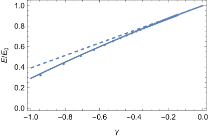
Figure 1: Energy of an attractive quasi-1D Fermi gas in the weakly attractive limit. The dots correspond to the exact solution the true 1D system using Bethe Ansatz’s solution (Eq. 4). The dashed line is the asymptotic solution incorporating the first beyond mean-field correction. We see that the agreement extends up to $|\gamma|\lesssim 1$.

III Quantum-simulation of Yang-Gaudin’s Hamiltonian

Experimentally, effective low dimensional physics is achieved by confining very strongly an ensemble of particles in one, two or three dimensions. When the typical single particle energies (ie chemical potential, temperature) are much smaller than the energy between the ground state and the first excited state of the trapping potential, it is usually assumed that the dynamics along the confined directions is frozen and that the system becomes effectively one- or two-dimensional, depending on the number of frozen directions Cazalilla et al. (2011). This mechanism is used in condensed matter physics, for instance at the junction between N- and P-doped semi-conductors in order to realize 2D-electron gases. In cold atoms, 1D and 2D vapours have been realized using optical trapping or magnetic trapping at the surface of atom chips.

In the ultracold regime, the de Broglie wave-length of the atoms is much larger than the range of the interatomic potential. As a consequence, interactions in free space can be accurately modeled using a zero-range contact potential characterized by a 3D scattering length $a_{3D}$. One would then naively expect that the low-energy physics in confined geometry would be described by a YG Hamiltonian, with a coupling constant $g_{1D}$ depending on $a_{3D}$ and the trap parameters.

Let’s consider a quasi-1D system described by the Hamiltonian

$$H=\sum_{i}\frac{p_{\sigma,i}^{2}}{2m}+\sum_{i,\sigma}\frac{m\omega_{\perp}^{2}}{2}(x_{\sigma,i}^{2}+y_{\sigma,i}^{2})+\sum_{i,j}V(\bm{r}_{\uparrow,i}-\bm{r}_{\downarrow,j})$$ (7)

where $V$ is the 3D interparticle interaction potential. Let’s note $E$ the energy of the ground-state. Assuming that the dynamics is indeed frozen in the $(x,y)$ plane, $E$ can be written as

$$E=N\hbar\omega_{\perp}+E_{\rm YG},$$ (8)

where $E_{\rm YG}$ is the ground state energy of the YG model with a 1D scattering length expressed in terms of $a_{3D}$ and $\ell_{\perp}=\sqrt{\hbar/m\omega_{\perp}}$. In the case of the two-body problem, the value of $a_{1D}$ was calculated in Olshanii (1998) and we have in this case:

$$a_{1D}=-\frac{\ell_{\perp}}{2}\left(\frac{\ell_{\perp}}{a_{3D}}+\zeta(1/2)\right),$$ (9)

where $\zeta$ is Riemann’s Zeta function. The transverse size of the cloud can be deduced from $E$ using Hellman-Feynman’s theorem. We have indeed:

$$\langle\rho^{2}\rangle=\frac{2}{Nm}\frac{\partial E}{\partial\omega_{\perp}^{2}},$$ (10)

where $\rho^{2}=x^{2}+y^{2}$. Since $E_{\rm YG}$ depends implicitly on $\omega_{\perp}$ through $a_{1D}$, we have

$$\langle\rho^{2}\rangle=\ell_{\perp}^{2}+\frac{1}{N}\frac{\partial a_{1D}}{\partial\ell_{\perp}}\frac{\partial E_{\rm YG}}{\partial a_{1D}}$$ (11)

The first term corresponds to the size of the ground state and in the second term we recognize the so-called Tan-contact parameter Tan (2008); Olshanii and Dunjko (2003). We can consider the system as effectively 1D if $\langle\rho^{2}\rangle$ stays close to $\ell_{\perp}^{2}$ (note that, paradoxically, compressing the transverse size below $\ell_{\perp}^{2}$ does not improve one-dimensionality. Indeed, due to Heisenberg’s uncertainty relations, this implies that additional transverse energy is stored as kinetic energy).

In the weakly interacting limit, we can use Eq. (6) to evaluate $E_{\rm YG}$ within the mean-field approximation. In this case, the transverse size of the system is given by

$$\langle\rho^{2}\rangle\simeq\ell_{\perp}^{2}\left(1-\frac{\ell_{\perp}^{2}}{a_{1D}^{2}}\frac{\partial a_{1D}}{\partial\ell_{\perp}}n\ell_{\perp}\right).$$ (12)

Interestingly, we see that when the density is small the correction to the non-interacting case can also be made arbitrary small thanks to the $n\ell_{\perp}$ contribution. In other words, In the mean-field regime, the transverse radius is consistent with a frozen motion in the transverse direction as long as the Fermi energy $E_{F}=\hbar^{2}(n\pi)^{2}/8m$ is sufficiently small compared to $\hbar\omega_{\perp}$ as expected from the naive interpretation of the quasi-1D regime.

Let’s now consider the strongly attractive limit (corresponding to a large $\gamma$). In this case, the 1D system is a gas of bosonic dimers and $E_{\rm YG}$ is dominated by their binding energies, ie

$$E_{\rm YG}\simeq-\frac{N\hbar^{2}}{2ma_{1D}^{2}}.$$ (13)

We then obtain

$$\langle\rho^{2}\rangle=\ell_{\perp}^{2}\left(1-\frac{\ell_{\perp}^{3}}{2a_{1D}^{3}}\frac{\partial a_{1D}}{\partial\ell_{\perp}}\right).$$ (14)

We see that in this case, the correction becomes density independent and as a consequence, a finite amount of energy remains stored in the transverse degrees of freedom, even when $E_{F}\ll\hbar\omega_{\perp}$. Close to the confinement-induced resonance where $a_{1D}$ vanishes, the correction even diverges. We conclude from this argument that the quasi-1D approximation is no longer valid when the system approaches the resonant $a_{3D}/\ell_{\perp}\rightarrow\infty$, and beyond.

The origin of this breakdown was outlined in past references Fuchs et al. (2004); Tokatly (2004); Mora et al. (2005): when entering the strongly attractive regime, the molecule binding energy becomes larger than $\hbar\omega_{\perp}$. As a consequence their internal structure is no longer affected by the transverse confining potential and becomes identical to that of molecules in free space. This phenomenon is more dramatically illustrated by the fact that in a quasi-1D geometry, there is a bound state for any value on the 3D scattering length, even when $a_{1D}$ is negative, which contradicts the fact that for a purely 1D system, bound state exist only for positive $a_{1D}$.

IV Effective Hamiltonian for quasi-1D fermions

Since Yang-Gaudin’s Hamiltonian ceases to apply for strong interactions, we focus on the weakly interacting regime and we explore its accuracy within a perturbative approach. According to Fig. (1), a calculation to second order in perturbation theory should be valid up to $\gamma\simeq 1$. Interactions give rise to both “intraband” processes, where all particles stay in the transverse ground state of the trapping potential, and “interband” collisions where one or more particles are virtually excited towards an excited state of the confining potential. It is well known that these virtual processes give rise to effective few-body interactions Goban et al. (2018) that we calculate in a many-body context using the Schrieffer-Wolff’s (SW) approach Schrieffer and Wolff (1966). The many-body Hamiltonian describing an ensemble of spin-1/2 fermionic atoms confined by a transverse external potential is given by

$$H=H_{0}+H_{\rm int},$$ (15)

In this expression, $H_{0}$ is the free particle Hamiltonian. In a second-quantized form, we write it as

$$H_{0}=\sum_{\alpha,\sigma}\epsilon(k,\alpha)a_{\sigma k\alpha}^{\dagger}a_{\sigma k\alpha}$$ (16)

where $\sigma$ is the spin index, $k$ is the momentum in the $z$ direction and $\alpha=(n,m_{z})$ labels the transverse state: $n$ is the quantum number associated with the energy of the transverse motion and $\hbar m_{z}$ is the angular momentum along $z$. For a harmonic confinement, $m_{z}\in\{-n,-n+2,...n-2,n\}$ and $\varepsilon(k,\alpha)=\hbar^{2}k^{2}/2m+\hbar\omega_{\perp}(n+1)$.

$H_{\rm int}$ describes the two-body interactions and is given by

$$H_{\rm int}=\frac{g_{3D}}{L}\sum_{\begin{subarray}{c}k_{1}+k_{2}=\\ k_{3}+k_{4}\\ (\alpha_{1}\alpha_{2}\alpha_{3}\alpha_{4})\end{subarray}}\chi_{\alpha_{1}\alpha_{2}\alpha_{3}\alpha_{4}}a^{\dagger}_{\uparrow k_{1}\alpha_{1}}a_{\uparrow k_{2}\alpha_{2}}a^{\dagger}_{\downarrow k_{3}\alpha_{3}}a_{\downarrow k_{4}\alpha_{4}},$$ (17)

where $g_{3D}=4\pi\hbar^{2}a_{3D}/m$ is the bare coupling constant and the matrix elements $\chi_{\alpha_{1}\alpha_{2}\alpha_{3}\alpha_{4}}$ are defined as

$$\chi_{\alpha_{1}\alpha_{2}\alpha_{3}\alpha_{4}}=\int d^{2}\bm{\rho}\psi_{\alpha_{1}}(\bm{\rho})^{*}\psi_{\alpha_{2}}(\bm{\rho})\psi_{\alpha_{3}}^{*}(\bm{\rho})\psi_{\alpha_{4}}(\bm{\rho}),$$ (18)

with $\psi_{\alpha}(\bm{\rho})$ being the wave function associated with the eigenstate $\alpha$ of the transverse motion.

To implement the Schrieffer-Wolff scheme, we write $H_{\rm int}=H_{1}+H_{2}$, where $H_{1}$ and $H_{2}$ correspond to intra- and interband processes, ie to contributions of $(\alpha_{1},\alpha_{2},\alpha_{3},\alpha_{4})=(0,0,0,0)$ and $(\alpha_{1},\alpha_{2},\alpha_{3},\alpha_{4})\not=(0,0,0,0)$ respectively.

Since $H_{2}$ is responsible to virtual interband transitions, we treat it perturbatively within SW approach. Lets define $\tilde{H}=H_{0}+H_{2}$. In the SW scheme we look for a canonical transformation $\tilde{H}^{\prime}=\exp(S)\tilde{H}\exp(-S)$ with generator $S$ such that $\tilde{H}^{\prime}$ becomes diagonal to first order in $H_{2}$. This amounts to requiring

$$[H_{0},S]=H_{2},$$ (19)

yielding

$$\tilde{H}^{\prime}=H_{0}+\frac{1}{2}[S,H_{2}]+\mathcal{O}(g_{3D}^{3}),$$ (20)

showing that the correction to the Hamiltonian $\tilde{H}$ is quadratic in the coupling constant as $S$ is linear in $g_{3D}$. The total Hamiltonian in the rotated basis is then given by

$$H^{\prime}=e^{S}He^{-S}=\tilde{H}^{\prime}+e^{S}H_{1}e^{-S}=H_{\rm eff}+\mathcal{O}(g_{3D}^{3}),$$ (21)

where

$$H_{\rm eff}=H_{0}+H_{1}+\frac{1}{2}[S,H_{2}]+[S,H_{1}]$$ (22)

is the perturbative effective Hamiltonian of the system that we are looking for. Notice that for $S=0$, the effective Hamiltonian reduces to the Yang-Gaudin model, since $H_{0}+H_{1}=H_{\rm YG}$.

In order to write $H_{\rm eff}$ explicitly in second quantization form, we need to find a representation of the generator $S$ in terms of the fermionic field operators. Since $H_{0}$ and $H_{2}$ are, respectively, quadratic and quartic in those fields, it is easy to see that Eq. (19) can only be satisfied if $S$ is a quartic operator of the form

$$S=\!\!\frac{g_{3D}}{L}\!\!\!\sum_{\begin{subarray}{c}k_{1},k_{2},k_{3},k_{4}\\ (\alpha_{1},\alpha_{2},\alpha_{3},\alpha_{4})\not=\\ (0,0,0,0)\end{subarray}}\!\!\!f(\{k_{i},\alpha_{i}\})a_{\uparrow k_{1}\alpha_{1}}^{\dagger}a_{\downarrow k_{3}\alpha_{3}}^{\dagger}a_{\downarrow k_{4}\alpha_{4}}a_{\uparrow k_{2}\alpha_{2}},$$ (23)

where $f(\{k_{i},\alpha_{i}\})$ is an unknown function of the four axial momenta $k_{i}$ and the four discrete indices $\alpha_{i}$ for the motion along the transverse directions. Notice that the term with all $\alpha_{i}=0$ in Eq.(23 does not mix with the excited states of the confining potential and therefore cannot contribute to the generator $S$ (otherwise $[H_{0},S]$ would also contain a similar term, which is instead absent in $H_{2}$, thus violating Eq.(19)).

In order to determine the function $f$, we substitute Eq.(23) into Eq.(19) and use the anticommutation relations $\{a_{\sigma k\alpha}^{\dagger},a_{\sigma^{\prime}p\alpha^{\prime}}\}=\delta_{\sigma\sigma^{\prime}}\delta_{kp}\delta_{\alpha\alpha^{\prime}}$, $\{a_{\sigma k\alpha},a_{\sigma^{\prime}p\alpha^{\prime}}\}=0$. This yields

$$f(\{k_{i},\alpha_{i}\})=\frac{\chi_{\alpha_{1}\alpha_{2}\alpha_{3}\alpha_{4}}\delta_{k_{1}+k_{3},k_{2}+k_{4}}}{\epsilon(k_{1},\alpha_{1})+\epsilon(k_{3},\alpha_{3})-\epsilon(k_{2},\alpha_{2})-\epsilon(k_{4},\alpha_{4})}.$$ (24)

The effective Hamiltonian can then be calculated by substituting Eq.s (23) and (24) in Eq. (22), and by evaluating the two commutators. The details of the derivation are given in Appendix A. In particular, since we are interested on the 1D effective theory describing atoms in the ground state of the harmonic oscillator, we consider only creation and annihilation operators with $\alpha=0$. This implies that $[S,H_{1}]$ does not contribute to the effective model while the contribution from the commutator $[S,H_{2}]$ can be recast as a sum of two parts, $[S,H_{2}]/2=H^{\prime}_{2}+H^{\prime\prime}_{2}$. The first part describes two-body interactions (containing only four creation and annihilation operators) and is given by

$$H^{\prime}_{2}=\frac{g_{3D}^{2}}{2L^{2}}\sum_{\begin{subarray}{c}k_{1}+k_{3}\\ =\\ p_{2}+p_{4}\end{subarray}}(F(k_{1},k_{3})+F(p_{2},p_{4}))\;a_{\uparrow k_{1}0}^{\dagger}a_{\downarrow k_{3}0}^{\dagger}a_{\downarrow p_{4}0}a_{\uparrow p_{2}0},$$ (25)

with

$$F(k_{1},k_{3})=\sum_{\begin{subarray}{c}k_{2},k_{4}\\ \alpha_{2}\alpha_{4}\end{subarray}}f(\{k_{i},\alpha_{i}\})\chi_{\alpha_{2}0\alpha_{4}0}.$$ (26)

The second part corresponds to emergent three-body interactions (containing products of six operators) and can be written as

$$\begin{split}&H^{\prime\prime}_{2}=\frac{g_{3D}^{2}}{2L^{2}}\sum_{\begin{subarray}{c}k_{1}+k_{3}+p_{3}\\ =\\ p_{2}+p_{4}+k_{4}\end{subarray}}\!\!\!\Big{[}\left(G(k_{1},k_{3},k_{4})+G(p_{2},p_{3},p_{4})\right)\times\\ &a_{\uparrow k_{1}0}^{\dagger}a_{\downarrow k_{3}0}^{\dagger}a_{\downarrow p_{3}0}^{\dagger}a_{\downarrow p_{4}0}a_{\downarrow k_{4}0}a_{\uparrow p_{2}0}+(\uparrow\leftrightarrow\downarrow)\Big{]},\end{split}$$ (27)

with

$$G(k_{1},k_{3},k_{4})=\sum_{k_{2}\alpha_{2}}f(\{k_{i},\alpha_{i}\})\chi_{\alpha_{2}000}.$$ (28)

V Effective two-body interactions

By construction, $H^{\prime\prime}_{2}$ in Eq. (27) does not contribute to the two-body sector. We reorganize the effective two-body interaction at low energy as $H_{1}+H^{\prime}_{2}=U^{\prime}+U^{\prime\prime}$ with

$$U^{\prime}=\frac{\tilde{g}_{1D}}{L}\sum_{k_{1}+k_{2}=p_{1}+p_{2}}a_{\uparrow k_{1}0}^{\dagger}a_{\downarrow k_{2}0}^{\dagger}a_{\downarrow p_{2}0}a_{\uparrow p_{1}0},$$ (29)

where the effective 1D coupling constant is given by

$$\begin{split}\tilde{g}_{1D}&=g_{3D}\chi_{0000}\\ &-\frac{g_{3D}^{2}}{L}\sum_{\begin{subarray}{c}k_{2}+k_{4}=0\\ \alpha_{1}\alpha_{2}\end{subarray}}\frac{\chi_{0\alpha_{1}0\alpha_{2}}^{2}}{\frac{\hbar^{2}k_{2}^{2}}{2m}+\frac{\hbar^{2}k_{4}^{2}}{2m}+\hbar\omega_{\perp}(n_{\alpha_{2}}+n_{\alpha_{4}})}.\end{split}$$ (30)

Strictly speaking, this sum is divergent (see appendix B). This is a consequence of the zero-range potential approximation that is notoriously known to be singular. The divergence can be cured by the introduction of a UV-cutoff and by considering $g_{3D}$ as a running coupling constant that vanishes when the cutoff goes to zero. If properly performed, this regularization procedure recovers the exact result derived in Olshanii (1998). Here, we wil take $\tilde{g}_{1D}$ as given and we will use it to renormalize all diverging quantities appearing in forthcoming calculations.

The remaining part of the two body interaction is given by

$$\begin{split}U^{\prime\prime}=\frac{g_{3D}^{2}}{2L^{2}}\sum_{k_{1}+k_{3}=p_{2}+p_{4}}&(F(k_{1},k_{3})+F(p_{2},p_{4})-2F(0,0))\\ &\times a_{\uparrow k_{1}0}^{\dagger}a_{\downarrow k_{3}0}^{\dagger}a_{\downarrow p_{4}0}a_{\uparrow p_{2}0}\end{split}$$ (31)

and describes finite-range/momentum-dependent corrections to the two-body interactions. Note that contrary to $\tilde{H}_{1}^{\prime}$, this term has a well-defined UV limit.

VI Effective three-body interaction

Let’s consider now the low-energy behaviour of the three-body interaction term $H_{2}^{\prime\prime}$. When taking $k_{1,3,4}=p_{2,3,4}=0$ in Eq. (27), the exchange of $k_{3}$ and $p_{3}$ on the one hand, and $k_{4}$ and $p_{4}$ on the other hand lead to a cancellation of $H^{\prime\prime}_{2}$. This is a departure from previous results on bosonic systems Mazets et al. (2008); Tan et al. (2010); Pricoupenko (2019) where the three-body coupling constant is momentum independent. Indeed, let’s consider a generic three-body interaction

$$\begin{split}&U_{3\rm b}=\sum_{\begin{subarray}{c}k_{1}+k_{3}+p_{3}\\ =\\ p_{2}+p_{4}+k_{4}\end{subarray}}\!\!\!\Big{[}K(\{k_{i},p_{j}\})\times\\ &a_{\uparrow k_{1}0}^{\dagger}a_{\downarrow k_{3}0}^{\dagger}a_{\downarrow p_{3}0}^{\dagger}a_{\downarrow p_{4}0}a_{\downarrow k_{4}0}a_{\uparrow p_{2}0}+(\uparrow\leftrightarrow\downarrow)\Big{]}\end{split}$$ (32)

If we expand the function $K$ to second order in momentum, we readily see that the lowest order term yielding a nonzero contribution because of fermionic exchange is

$$K\propto(k_{3}-p_{3})(k_{4}-p_{4}).$$ (33)

This result can also be recovered directly by calculating the low momentum asymptotic behaviour of Eq. (28). For this, we take $k_{1}=p_{2}=0$ in $G$ and then expand it to first order in $k_{3,4}$ and $p_{3,4}$. We then obtain

$$\begin{split}&H^{\prime\prime}_{2}=-\frac{\hbar^{2}a_{3D}^{2}}{4mL^{2}}{\rm Li}_{1/2}(1/4)\sum_{\begin{subarray}{c}k_{1}+k_{3}+p_{3}\\ =\\ p_{2}+p_{4}+k_{4}\end{subarray}}\!\!\!\Big{[}(k_{3}-p_{3})(k_{4}-p_{4})\times\\ &a_{\uparrow k_{1}0}^{\dagger}a_{\downarrow k_{3}0}^{\dagger}a_{\downarrow p_{3}0}^{\dagger}a_{\downarrow p_{4}0}a_{\downarrow k_{4}0}a_{\uparrow p_{2}0}+(\uparrow\leftrightarrow\downarrow)\Big{]}\end{split}$$ (34)

where ${\rm Li}_{s}(z)=\sum_{n=1}^{\infty}z^{n}/n^{s}$ is the polylog function and where with have used Appendix B to calculate the sum over $\alpha_{2}$.

VII Ground state energy

Let us now calculate the interaction-induced correction to the ground state energy of the effective Hamiltonian (22) and verify that we recover the same result by applying perturbation theory to the original Hamiltonian $H$. The noninteracting ground state of the system is given by the product of the Fermi seas of the two spin components, $|FS\rangle=|FS_{\uparrow}\rangle|FS_{\downarrow}\rangle$, where

$$|FS_{\sigma}\rangle=\prod_{|k|<k_{F\sigma}}a_{\sigma k0}^{\dagger}|\rangle,$$ (35)

where $|\rangle$ represents the vacuum state and $k_{F\sigma}$ are the Fermi momentum of the spin component $\sigma=\uparrow,\downarrow$.

Since the two-body and three-body terms of the effective Hamiltonian arising from the commutator $[H,S_{2}]$ are proportional to $g_{3D}^{2}$, we treat them within first order perturbation theory.

Making use of the identities

$$\begin{split}&\langle FS_{\sigma}|a_{\sigma k_{1}0}^{\dagger}a_{\sigma p_{2}0}|FS_{\sigma}\rangle=\Theta(k_{F\sigma}-|k_{1}|)\delta_{k_{1}p_{2}}\\ &\langle FS_{\sigma}|a_{\sigma k_{3}0}^{\dagger}a_{\sigma p_{3}0}^{\dagger}a_{\sigma p_{4}0}a_{\sigma k_{4}0}|FS_{\sigma}\rangle=\Theta(k_{F\sigma}-|k_{4}|)\\ &\quad\quad\times\Theta(k_{F\sigma}-|p_{4}|)(\delta_{p_{3}p_{4}}\delta_{k_{3}k_{4}}-\delta_{p_{3}k_{4}}\delta_{k_{3}p_{4}}),\end{split}$$ (36)

we obtain

$$\begin{split}&\!\!\!\!\!\!\!\!\!\langle FS|\frac{1}{2}[S,H_{2}]|FS\rangle=\frac{g_{3D}^{2}}{L^{2}}\Bigg{[}\;\sum_{\begin{subarray}{c}|k_{1}|<k_{F\uparrow}\\ |k_{3}|<k_{F\downarrow}\end{subarray}}F(k_{1},k_{3})\\ &\!\!\!\!\!\!\!\!-\sum_{\begin{subarray}{c}|k_{1}|<k_{F\uparrow}\\ |k_{3}|,|k_{4}|<k_{F\downarrow}\end{subarray}}\!\!G(k_{1},k_{3},k_{4})-\sum_{\begin{subarray}{c}|k_{1}|,|k_{2}|<k_{F\uparrow}\\ |k_{3}|<k_{F\downarrow}\end{subarray}}\!\!G(k_{1},k_{3},k_{2})\\ &\!\!\!\!\!\!\!+\!\!\!\sum_{\begin{subarray}{c}|k_{1}|<k_{F\uparrow}\\ |k_{3}|,|p_{4}|<k_{F\downarrow}\end{subarray}}\!\!G(k_{1},k_{3},k_{3})+\!\!\!\!\!\!\sum_{\begin{subarray}{c}|k_{1}||p_{1}|<k_{F\uparrow}\\ |k_{3}|<k_{F\downarrow}\end{subarray}}\!\!\!\!G(k_{1},k_{3},k_{1})\Bigg{]}.\end{split}$$ (37)

Notice that the rhs of Eq. (37) contains terms, where two of the arguments of the function $G$ become identical. From Eq.(28) we see that in this case the function reduces to a constant

$$G(k_{1},k_{3},k_{3})=\sum_{m_{2}\not=0}-\frac{|\chi_{0m_{2}00}|^{2}}{m_{2}\hbar\omega}.$$ (38)

Next, we turn to the correction $\delta E$ to the ground state energy due to $H_{1}$. Since this term is linear in $g_{3D}$, we will use second order perturbation theory

$$\delta E=\langle FS|H_{1}|FS\rangle+\sum_{n}\frac{|\langle n|H_{1}|FS\rangle|^{2}}{E_{FS}-E_{n}},$$ (39)

where $E_{FS}$ is the energy of the Fermi sea and $|n\rangle$ is a generic excited eigenstate of $H_{0}$, which is coupled to the ground state by $H_{1}$. From Eq.(36) we find that the correction linear in $g_{3D}$ is given by

$$\langle FS|H_{1}|FS\rangle=\frac{g_{3D}}{L}\chi_{0000}\sum_{\begin{subarray}{c}|k_{1}|<k_{F\uparrow}\\ |p_{3}|<k_{F\downarrow}\end{subarray}}=\frac{g_{3D}}{L}\chi_{0000}N_{\uparrow}N_{\downarrow},$$ (40)

which corresponds to the mean field.

The relevant excited states in the rhs of Eq. (39) correspond to particle-hole excitations $|n\rangle=a_{\uparrow k_{1}0}^{\dagger}a_{\downarrow k_{3}0}^{\dagger}a_{\downarrow k_{4}0}a_{\uparrow k_{2}0}|FS\rangle$, with the initial states $k_{2},k_{4}$ being inside the respective Fermi surfaces, $|k_{2}|<k_{F\uparrow},|k_{4}|<k_{F\downarrow}$, while the final states $k_{1},k_{3}$ are scattered outside them, $|k_{1}|>k_{F\uparrow},|k_{3}|>k_{F\downarrow}$. From Eq.(36) we then find

$$\langle n|H_{1}|FS\rangle=\frac{g_{3D}}{L}\chi_{0000}\delta_{k_{1}+k_{3},k_{2}+k_{4}}.$$ (41)

The change in the kinetic energy of the system brought by the excitation, appearing in the second order correction in Eq.(39), is given by

$$E_{n}-E_{FS}=\frac{\hbar^{2}k_{1}^{2}}{2m}+\frac{\hbar^{2}k_{3}^{2}}{2m}-\frac{\hbar^{2}k_{2}^{2}}{2m}-\frac{\hbar^{2}k_{4}^{2}}{2m}.$$ (42)

Finally, we write down the perturbative expansion $E=E_{FS}+\langle FS|[S,H_{2}]/2|FS\rangle+\delta E$ for the ground state energy for a system of equal spin populations, $N_{\uparrow}=N_{\downarrow}=N/2$, corresponding to $k_{F\uparrow}=k_{F\downarrow}=k_{F}/2$. Making use of Eq.s (49)-(50), together with Eq.s (37)-(42), we find

$$\begin{split}&E=E_{FS}+\frac{g_{3D}}{4L}\chi_{0000}N^{2}-\frac{g_{3D}^{2}}{L^{2}}\sum_{\begin{subarray}{c}|k_{1}|,|k_{3}|>k_{F}\\ |k_{2}|,|k_{4}|<k_{F}\end{subarray}}\frac{\chi_{0000}^{2}\delta_{k_{1}+k_{3},k_{2}+k_{4}}}{\frac{\hbar^{2}k_{1}^{2}}{2m}+\frac{\hbar^{2}k_{3}^{2}}{2m}-\frac{\hbar^{2}k_{2}^{2}}{2m}-\frac{\hbar^{2}k_{4}^{2}}{2m}}\\ &+\frac{g_{3D}^{2}}{L^{2}}\sum_{|k_{1}|,|k_{3}|<k_{F}}\sum_{\begin{subarray}{c}k_{2},k_{4}\\ (n_{\alpha_{2}},n_{\alpha_{4}})\not=(0,0)\end{subarray}}\frac{|\chi_{0\alpha_{2}0\alpha_{4}}|^{2}\delta_{k_{1}+k_{3},k_{2}+k_{4}}}{\frac{\hbar^{2}k_{1}^{2}}{2m}+\frac{\hbar^{2}k_{3}^{2}}{2m}-\frac{\hbar^{2}k_{2}^{2}}{2m}-\frac{\hbar^{2}k_{4}^{2}}{2m}-(n_{\alpha_{2}}+n_{\alpha_{4}})\hbar\omega}\\ &-2\frac{g_{3D}^{2}}{L^{2}}\sum_{\begin{subarray}{c}|k_{1}|<k_{F}\\ |k_{3}|,|k_{4}|<k_{F}\end{subarray}}\sum_{k_{2},n_{\alpha_{2}}\not=0}\frac{|\chi_{0m_{2}00}|^{2}\delta_{k_{1}+k_{3},k_{2}+k_{4}}}{\frac{\hbar^{2}k_{1}^{2}}{2m}+\frac{\hbar^{2}k_{3}^{2}}{2m}-\frac{\hbar^{2}k_{2}^{2}}{2m}-\frac{\hbar^{2}k_{4}^{2}}{2m}-n_{\alpha_{2}}\hbar\omega}-\frac{g_{3D}^{2}N^{3}}{4L^{2}}\sum_{n_{\alpha_{2}}\not=0}\frac{|\chi_{0m_{2}00}|^{2}}{n_{\alpha_{2}}\hbar\omega}\end{split}$$ (43)

The second sum appearing in the rhs of Eq. (43) is divergent. Following the prescription outlined in Sec. V, this singularity can be cured by noting that its structure is similar to the one of the divergent term of the two-body effective coupling constant $\tilde{g}_{1D}$. Indeed, the first three terms of the energy are similar to Eq. (5) for a purely 1D system with a coupling constant constant $g_{1D}=g_{3D}\chi_{0000}/L$. We can recover the same energy, but with the true coupling constant $\tilde{g}_{1D}$ by adding and subtracting the missing divergent term. We then have

$$\begin{split}E=E_{\rm YG}(\tilde{g}_{1D})&+\frac{g_{3D}^{2}}{L^{2}}\sum_{\begin{subarray}{c}|k_{1}|,|k_{3}|<k_{F}\\ k_{2}+k_{4}=k_{1}+k_{3}\\ (\alpha_{2},\alpha_{4})\not=(0,0)\end{subarray}}\left[\frac{|\chi_{0\alpha_{2}0\alpha_{4}}|^{2}}{\frac{\hbar^{2}k_{13}}{m}-\frac{\hbar^{2}k_{24}^{2}}{m}-(n_{\alpha_{2}}+n_{\alpha_{4}})\hbar\omega}+\frac{|\chi_{0\alpha_{2}0\alpha_{4}}|^{2}}{\frac{\hbar^{2}k_{24}^{2}}{m}+(n_{\alpha_{2}}+n_{\alpha_{4}})\hbar\omega}\right]\\ &-2\frac{g_{3D}^{2}}{L^{2}}\sum_{\begin{subarray}{c}|k_{1}|<k_{F}\\ |k_{3}|,|k_{4}|<k_{F}\\ k_{2}+k_{4}=k_{1}+k_{3}\\ \alpha_{2}\not=0\end{subarray}}\left[\frac{|\chi_{0\alpha_{2}00}|^{2}}{\frac{\hbar^{2}k_{13}^{2}}{m}-\frac{\hbar^{2}k_{24}^{2}}{m}-n_{\alpha_{2}}\hbar\omega}+\frac{|\chi_{0\alpha_{2}00}|^{2}}{n_{\alpha_{2}}\hbar\omega}\right]\end{split}$$ (44)

where $E_{\rm YG}(\tilde{g}_{1D})$ is the second order expansion of the energy of a 1D system with a coupling constant $\tilde{g}_{1D}$ given by Eq. (30) and $k_{ij}=(k_{i}-k_{j})/2$ is the relative momentum of the pair.

Since the corrections are proportional to $g_{3D}^{2}$, they will scale as $\gamma^{2}$. We can write the full energy as

$$E=E_{\rm YG}(\tilde{g}_{1D})\left[1-(A_{\rm 2b}+A_{\rm 3b})\gamma^{2}\right],$$ (45)

where the first term comes from finite range corrections and the second one from three-body interactions. The sum appearing in Eq. (44) can be calculated analytically in the quasi-1D limit $E_{F}\ll\hbar\omega_{\perp}$ (see appendix B) and we have

$$A_{2\rm b} \simeq \frac{\zeta(3/2)}{2\pi^{3}}\left(\frac{E_{F}}{\hbar\omega_{\perp}}\right)^{3/2}$$ (46)

$$A_{3\rm b} \simeq \frac{8}{\pi^{4}}{\rm Li}_{2}(1/4)\left(\frac{E_{F}}{\hbar\omega_{\perp}}\right)^{2}$$ (47)

where $\zeta$ is Riemann’s zeta function and where ${\rm Li}_{s}(z)$ is a polylog function as before . These asymptotic behaviours are compared to numerical calculations in Fig. 2. The approximate result provides an accurate value for $A_{\rm 3b,2b}$, even for $E_{F}\simeq\hbar\omega_{\perp}$ in the case of two-body interactions. We also note that the two body-contribution always dominate its three-body counterpart. Finally, even when for $E_{F}\simeq\hbar\omega_{\perp}$, both ${A_{2b}}$ and $A_{3b}$ do not exceed $\simeq 5\times 10^{-2}$, which suggests that virtual transitions affect only weakly the first beyond-mean-field corrections to the energy.

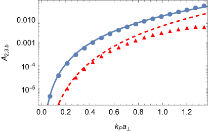
Figure 2: Contributions of 2 and 3-body effective interactions to the first beyond-mean-field corrections. Blue circles: 2 body contribution, Blue solid line: asymptotic expression (46). Red triangle: three body contribution $A_{3b}$. Red dashed line: asymptotic expression (47).

VIII Discussion

In this article we have calculated derived the effective many-body Hamiltonian describing a quasi-1D cloud of spin 1/2 fermions. We have calculated the first beyond mean-field corrections to the energy of a cloud of spin 1/2 fermions confined in a quantum wire. Our work extend to the fermionic many-body regime previous results on the few-body bosonic problem in quasi 1D. We have shown that, even for Fermi energies close to $\hbar\omega_{\perp}$ the corrections due to virtual transitions towards transverse excited states are rather small up to $\gamma\simeq 1$ where our calculation provides an accurate estimate for the energy. This means that experiments using cold atoms in quantum wires provide an accurate description of the ground state of Yang-Gaudin’s Hamiltonian that the most important source of discrepancy with pure one-dimensional physics will most likely be the occupation of transverse excited states due to the finite temperature of the system. It would then be interesting to connect our work to high temperatures results obtained using Virial expansion Kristensen et al. (2016).

Even though the Yang-Gaudin provides a good description of the weakly-interacting regime, we have shown that it fails in the strongly attractive limit. In future work we will therefore extend our calculation to the non-perturbative limit to explore the breakdown of the 1D effective regime. Another intriguing research direction would be to generalize our results to quasi-2D systems where puzzling results showing deviations between experiments and 2D theories have been reported in Sobirey et al. (2021).

Appendix A Derivation of the effective Hamiltonian

We provide below the second quantization expression of the effective Hamiltonian $H_{\rm eff}$ obtained via the SW transformation. To this end, we substitute the explicit form of the generator $S$, given in Eq.s (23) and (24), into Eq.(22) and evaluate the two commutators $[S,H_{1}]$ and $[S,H_{2}]$. The action of each commutator can be written as a sum of two parts: the first part contains all contributions with products of four field operators and therefore renormalizes two-body interactions, while the second part gathers all contributions with products of six field operators, thus describing effective three-body interactions. For the commutator involving $H_{2}$, an explicit calculation yields

$$\begin{split}&\frac{1}{2}[S,H_{2}]=\frac{g_{3D}^{2}}{2L^{2}}\Bigg{[}\;\sum_{\begin{subarray}{c}k_{1}+k_{3}=p_{2}+p_{4}\\ \ \alpha_{1},\alpha_{3},\beta_{2},\beta_{4}\end{subarray}}\left[F_{\alpha_{1}\alpha_{3}}^{\beta_{2}\beta_{4}}(k_{1},k_{3})+\bar{F}_{\beta_{2}\beta_{4}}^{\alpha_{1}\alpha_{3}}(p_{2},p_{4})\right]\;a_{\uparrow k_{1}\alpha_{1}}^{\dagger}a_{\downarrow k_{3}\alpha_{3}}^{\dagger}a_{\downarrow p_{4}\beta_{4}}a_{\uparrow p_{2}\beta_{2}}\\ &+\sum_{\begin{subarray}{c}k_{1}+k_{3}+p_{3}=p_{2}+p_{4}+k_{4}\\ \alpha_{1},\alpha_{3},\alpha_{4},\beta_{2},\beta_{3},\beta_{4}\end{subarray}}\!\!\!\left[G_{\alpha_{1}\alpha_{3}\alpha_{4}}^{\beta_{2}\beta_{3}\beta_{4}}(k_{1},k_{3},k_{4})+\bar{G}_{\beta_{2}\beta_{4}\beta_{3}}^{\alpha_{1}\alpha_{3}\alpha_{4}}(p_{2},p_{4},p_{3})\right]\left(a_{\uparrow k_{1}\alpha_{1}}^{\dagger}a_{\downarrow k_{3}\alpha_{3}}^{\dagger}a_{\downarrow p_{3}\beta_{3}}^{\dagger}a_{\downarrow p_{4}\beta_{4}}a_{\downarrow k_{4}\alpha_{4}}a_{\uparrow p_{2}\alpha_{2}}+(\uparrow\leftrightarrow\downarrow)\right)\Bigg{]},\end{split}$$ (48)

where the overbar stands for complex conjugation and we have introduced the functions

$$F_{\alpha_{1}\alpha_{3}}^{\beta_{2}\beta_{4}}(k_{1},k_{3})=\sum_{k_{2}k_{4}\alpha_{2}\alpha_{4}}f(\{k_{i},\alpha_{i}\})\chi_{\alpha_{2}\beta_{2}\alpha_{4}\beta_{4}}\;\;\;\\$$ (49)

$$G_{\alpha_{1}\alpha_{3}\alpha_{4}}^{\beta_{2}\beta_{3}\beta_{4}}(k_{1},k_{3},k_{4})=\sum_{k_{2}\alpha_{2}}f(\{k_{i},\alpha_{i}\})\chi_{\alpha_{2}\beta_{2}\beta_{3}\beta_{4}}.$$ (50)

A similar calculation for the commutator $[S,H_{1}]$ gives

$$[S,H_{1}] = \frac{g_{3D}^{2}}{L^{2}}\sum_{\begin{subarray}{c}k_{1}+k_{3}=p_{2}+p_{4}\\ (m_{1},m_{3})\not=(0,0)\end{subarray}}\Big{[}R_{\alpha_{1}\alpha_{3}}(k_{1},k_{3})a_{\uparrow k_{1}\alpha_{1}}^{\dagger}a_{\downarrow k_{3}\alpha_{3}}^{\dagger}a_{\downarrow p_{4}0}a_{\uparrow p_{2}0}+\bar{R}_{\alpha_{1}\alpha_{3}}(k_{1},k_{3})a_{\uparrow p_{2}0}^{\dagger}a_{\downarrow p_{4}0}^{\dagger}a_{\downarrow k_{3}\alpha_{3}}a_{\uparrow k_{1}\alpha_{1}}\Big{]}$$ (51)

$$+ \frac{g_{3D}^{2}}{L^{2}}\sum_{\begin{subarray}{c}k_{1}+k_{3}+p_{3}=p_{2}+p_{4}+k_{4}\\ (\alpha_{1},\alpha_{3},\alpha_{4})\not=(0,0,0)\end{subarray}}\Bigg{[}T_{\alpha_{1}\alpha_{3}\alpha_{4}}(k_{1},k_{3},k_{4})\left(a_{\downarrow k_{4}\alpha_{4}}^{\dagger}a_{\downarrow p_{4}0}^{\dagger}a_{\downarrow p_{3}0}a_{\downarrow k_{3}\alpha_{3}}a_{\uparrow k_{1}\alpha_{1}}+(\uparrow\leftrightarrow\downarrow)\right)\Bigg{]},$$

where we have introduced the functions

$$T_{\alpha_{1}\alpha_{3}\alpha_{4}}(k_{1},k_{3},k_{4})=\sum_{k_{2}}\chi_{\alpha_{1}0\alpha_{3}\alpha_{4}}\chi_{0000}\delta_{k_{1}+k_{3},k_{2}+k_{4}}$$

$$\!\!\!\times\frac{1}{\epsilon(k_{1},\alpha_{1})+\epsilon(k_{3},\alpha_{3})-\epsilon(k_{2},0)-\epsilon(k_{4},\alpha_{4})}\quad$$ (52)

and

$$R_{\alpha_{1}\alpha_{3}}(k_{1},k_{3})=\sum_{k_{4}}T_{\alpha_{1}\alpha_{3}0}(k_{1},k_{3},k_{4}).$$ (53)

Notice that the Hamiltonian correction in Eq.(51) does not contribute to the ground state energy of the system, because it does not contain terms with all $\alpha_{i}=0$.

Appendix B Calculation of the sums appearing in the two- and three-body effective interactions

When calculating the energy of the quasi-1D gas in Eq. (44), two types of sums appear. Firstly, we have terms involving $\chi_{0\alpha 00}$. This matrix element can be explicitly written as

$$\chi_{0\alpha 00}=\int d^{2}\bm{\rho}\psi_{0}(\bm{\rho})^{3}\psi_{\alpha}(\bm{\rho}).$$

where we have used the fact that the ground-state wavefunction $\psi_{0}$ is real. Since the ground state of the 2D harmonic oscillator is isotropic we first see that the function $\psi_{\alpha}$ must correspond to a null angular momentum. In this case $n_{\alpha}$ is necessarily even and we can then write, using the general properties of the 2D harmonic oscillator

$$\psi_{\alpha}(\rho)=\frac{1}{\sqrt{\pi}a_{\perp}}L_{n_{\alpha}/2}(\rho^{2}/a_{\perp}^{2})e^{-\rho^{2}/2a_{\perp}^{2}},$$

where $L_{n}(x)$ is the Laguerre polynomial of order $n$.

Taking $u=\rho^{2}/a_{\perp}^{2}$, we have thus

$$\chi_{0\alpha 00}=\frac{1}{\pi a_{\perp}^{2}}\int duL_{n_{\alpha}/2}(u)e^{-2u}=\frac{1}{2\pi a_{\perp}^{2}}\frac{1}{2^{n_{\alpha}/2}},$$

where we have used the value of the Laplace transform of a Laguerre polynomial

$$\int_{0}^{\infty}due^{-su}L_{n}(u)=\frac{1}{s}\left(\frac{s-1}{s}\right)^{n}.$$

Thanks to the exponential decay $\chi_{0\alpha 00}$, the associated sum over $\alpha$ appearing in Eq. (44) converges.

The second type of sum has the general structure

$$A(z) = \sum_{\alpha_{1}\alpha_{2}}\frac{|\chi_{0\alpha_{1}0\alpha_{2}}|^{2}}{z-\hbar\omega_{\perp}(n_{\alpha_{1}}+n_{\alpha_{2}})}$$ (54)

$$= \sum_{\alpha_{1}\alpha_{2}}\frac{|\langle\alpha_{1}\alpha_{2}|\delta(\bm{\rho}_{12})|00\rangle|^{2}}{z-\hbar\omega_{\perp}(n_{\alpha_{1}}+n_{\alpha_{2}})}.$$ (55)

with $\bm{\rho}_{12}=\bm{\rho}_{1}-\bm{\rho}_{2}$. Noting that the sum is actually a completeness relation, this expression can be recast as

$$\langle 00|\delta(\bm{\rho}_{12})\frac{1}{z+2\hbar\omega_{\perp}-h_{1}-h_{2}}\delta(\bm{\rho}_{12})|00\rangle,$$

where $h_{i}$ is the transverse harmonic oscillator Hamiltonian describing the dynamics of particle $i$ in the $(x,y)$ plane, up to a constant to set the ground state energy at 0. Instead of describing the state of the system using the coordinates of the two particles, we can consider the relative and center of mass degrees of freedom of the pair of atoms. In this case the Hamitonian $h_{1}+h_{2}$ can be written as a sum of two harmonic oscillator $h_{r}$ and $h_{c}$ associated respectively with the relation and center of mass motion of the pair. They correspond to harmonic oscillators of the same frequency $\omega_{\perp}$ and masses $\mu=m/2$ and $M=2m$. If we insert a completeness relation for the new basis $|\alpha_{r},\alpha_{c}\rangle$, we note that since $\delta(\bm{\rho}_{12})$ acts only on the relative motion, we do not have any contirbution of the center of mass degrees of freedom and the sum can be written as

$$A(z)=\sum_{\alpha_{r}}\frac{|\langle\alpha_{r}|\delta(\bm{\rho}_{12})|0\rangle|^{2}}{z-\hbar\omega_{\perp}n_{\alpha_{r}}}=\sum_{\alpha_{r}}\frac{|\psi_{\alpha_{r}}(0)\psi_{0}(0)|^{2}}{z-\hbar\omega_{\perp}n_{\alpha_{r}}}$$

Since the sum depends only on the value of the wavefunction in $\bm{\rho}_{12}=0$, it means that only the zero-angular momentum modes contribute. In this case, $n_{\alpha_{r}}$ is even and $\psi_{\alpha_{r}}(0)=1/\sqrt{2\pi}a_{\perp}$. We finally have

$$A(z)=\frac{1}{(2\pi)^{2}a_{\perp}^{4}}\sum_{n=0}^{\infty}\frac{1}{z-2\hbar\omega_{\perp}n}$$

Strictly speaking, this sum is divergent. However, in Eq. (44), we take the difference of two terms having the same structure and compensating at large $n$. Note also that in that equation, the sum over $(\alpha_{1},\alpha_{2})$ excludes the ground state, which amounts to starting the sum over $n$ at $n=1$.

References

- Bloch et al. (2008) I. Bloch, J. Dalibard, and W. Zwerger, Rev. Mod. Phys. 80, 885 (2008).
- Georgescu et al. (2014) I. M. Georgescu, S. Ashhab, and F. Nori, Reviews of Modern Physics 86, 153 (2014), ISSN 15390756, URL https://journals.aps.org/rmp/abstract/10.1103/RevModPhys.86.153.
- Zwerger (2012) W. Zwerger, ed., The BCS-BEC Crossover and the Unitary Fermi Gas, vol. 836 of Lecture Notes in Physics (Springer, Berlin, 2012).
- Browaeys and Lahaye (2020) A. Browaeys and T. Lahaye, Nature Physics 2020 16:2 16, 132 (2020), ISSN 1745-2481, URL https://www.nature.com/articles/s41567-019-0733-z.
- De Daniloff et al. (2021) C. De Daniloff, M. Tharrault, C. Enesa, C. Salomon, F. Chevy, T. Reimann, and J. Struck (2021), URL http://arxiv.org/abs/2102.01589.
- Moritz et al. (2005) H. Moritz, T. Stöferle, K. Günter, M. Köhl, and T. Esslinger, Phys. Rev. Lett. 94, 210401 (2005).
- Orso (2007) G. Orso, Phys. Rev. Lett. 98, 70402 (2007).
- Hu et al. (2007) H. Hu, X.-J. Liu, and P. D. Drummond, Phys. Rev. Lett. 98, 70403 (2007).
- Parish et al. (2007) M. M. Parish, S. K. Baur, E. J. Mueller, and D. A. Huse, Phys. Rev. Lett. 99, 250403 (2007).
- Liao et al. (2010) Y. Liao, A. S. C. Rittner, T. Paprotta, W. Li, G. B. Partridge, R. G. Hulet, S. K. Baur, and E. J. Mueller, Nature 467, 567 (2010).
- Revelle et al. (2016) M. C. Revelle, J. A. Fry, B. A. Olsen, and R. G. Hulet, Physical review letters 117, 235301 (2016).
- Pagano et al. (2014) G. Pagano, M. Mancini, G. Cappellini, P. Lombardi, F. Schäfer, H. Hu, X.-J. Liu, J. Catani, C. Sias, M. Inguscio, et al., Nature Physics 10, 198 (2014).
- Yang et al. (2018) T. L. Yang, P. Grišins, Y. T. Chang, Z. H. Zhao, C. Y. Shih, T. Giamarchi, and R. G. Hulet, Physical review letters 121, 103001 (2018).
- He et al. (2020) F. He, Y. Z. Jiang, H. Q. Lin, R. G. Hulet, H. Pu, and X. W. Guan, Physical Review Letters 125, 190401 (2020), ISSN 10797114, URL https://journals.aps.org/prl/abstract/10.1103/PhysRevLett.125.190401.
- Guan et al. (2013) X.-W. Guan, M. T. Batchelor, and C. Lee, Reviews of Modern Physics 85, 1633 (2013).
- Mazets et al. (2008) I. E. Mazets, T. Schumm, and J. Schmiedmayer, Phys. Rev. Lett. 100, 210403 (2008), URL https://link.aps.org/doi/10.1103/PhysRevLett.100.210403.
- Tan et al. (2010) S. Tan, M. Pustilnik, and L. I. Glazman, Phys. Rev. Lett. 105, 90404 (2010), URL https://link.aps.org/doi/10.1103/PhysRevLett.105.090404.
- Pricoupenko (2019) L. Pricoupenko, Phys. Rev. A 99, 12711 (2019), URL https://link.aps.org/doi/10.1103/PhysRevA.99.012711.
- Goban et al. (2018) A. Goban, B. Hutson, G. E. Marti, S. L. Campbell, M. A. Perlin, P. S. Julienne, J. P. D’incao, A. M. Rey, and J. Ye, Nature (2018), URL https://doi.org/10.1038/s41586-018-0661-6.
- Fuchs et al. (2004) J. N. Fuchs, A. Recati, and W. Zwerger, Physical Review Letters 93 (2004), ISSN 00319007.
- Tokatly (2004) I. V. Tokatly, Physical Review Letters 93, 090405 (2004), ISSN 00319007, URL https://journals.aps.org/prl/abstract/10.1103/PhysRevLett.93.090405.
- Mora et al. (2005) C. Mora, A. Komnik, R. Egger, and A. O. Gogolin, Physical Review Letters 95 (2005), ISSN 00319007.
- Schrieffer and Wolff (1966) J. R. Schrieffer and P. A. Wolff, Physical Review 149, 491 (1966), ISSN 0031899X, URL https://journals.aps.org/pr/abstract/10.1103/PhysRev.149.491.
- Gaudin (1967) M. Gaudin, Physics Letters A 24, 55 (1967), ISSN 0375-9601.
- Yang (1967) C. N. Yang, Physical Review Letters 19, 1312 (1967), ISSN 00319007, URL https://journals.aps.org/prl/abstract/10.1103/PhysRevLett.19.1312.
- Iida and Wadati (2007) T. Iida and M. Wadati, Journal of Statistical Mechanics: Theory and Experiment 2007, P06011 (2007), ISSN 1742-5468, URL https://iopscience.iop.org/article/10.1088/1742-5468/2007/06/P06011https://iopscience.iop.org/article/10.1088/1742-5468/2007/06/P06011/meta.
- Krivnov and Ovchinnikov (1975) V. Y. Krivnov and A. Ovchinnikov, Soviet Journal of Experimental and Theoretical Physics 40, 781 (1975).
- Mariño and Reis (2019) M. Mariño and T. Reis, Journal of Statistical Physics 177, 1148 (2019), ISSN 15729613, URL https://link.springer.com/article/10.1007/s10955-019-02413-1.
- Cazalilla et al. (2011) M. A. Cazalilla, R. Citro, T. Giamarchi, E. Orignac, and M. Rigol, Reviews of Modern Physics 83, 1405 (2011).
- Olshanii (1998) M. Olshanii, Physical Review Letters 81, 938 (1998).
- Tan (2008) S. Tan, Ann. Phys. 323, 2971 (2008).
- Olshanii and Dunjko (2003) M. Olshanii and V. Dunjko, Physical Review Letters 91, 090401 (2003), ISSN 10797114, URL https://journals.aps.org/prl/abstract/10.1103/PhysRevLett.91.090401.
- Kristensen et al. (2016) T. Kristensen, X. Leyronas, and L. Pricoupenko, Physical Review A 93, 063636 (2016), ISSN 24699934, URL https://journals.aps.org/pra/abstract/10.1103/PhysRevA.93.063636.
- Sobirey et al. (2021) L. Sobirey, H. Biss, N. Luick, M. Bohlen, H. Moritz, and T. Lompe, ArXiv preprint: 2106.11893v1 (2021).