Bayesian sequential design of computer experiments for quantile set inversion

Abstract

We consider an unknown multivariate function representing a system—such as a complex numerical simulator—taking both deterministic and uncertain inputs. Our objective is to estimate the set of deterministic inputs leading to outputs whose probability (with respect to the distribution of the uncertain inputs) of belonging to a given set is less than a given threshold. This problem, which we call Quantile Set Inversion (QSI), occurs for instance in the context of robust (reliability-based) optimization problems, when looking for the set of solutions that satisfy the constraints with sufficiently large probability. To solve the QSI problem, we propose a Bayesian strategy based on Gaussian process modeling and the Stepwise Uncertainty Reduction (SUR) principle, to sequentially choose the points at which the function should be evaluated to efficiently approximate the set of interest. We illustrate the performance and interest of the proposed SUR strategy through several numerical experiments.

 

 

Keywords: Gaussian processes, Active learning, Design of computer experiments, Stepwise Uncertainty Reduction, Set inversion, Uncertainty quantification.

1 Introduction

When dealing with a numerical model of a physical phenomenon or a system, one is often interested in estimating the set of input parameters leading to outputs in a given range. Such set inversion problems (Jaulin and Walter, 1993) arise in a large variety of frameworks. In particular, “robust” formulations of the set inversion problem, in which some inputs are considered uncertain, have appeared recently in the literature, with applications to nuclear safety (Chevalier, 2013; Marrel et al., 2022), flood defense optimization (Richet and Bacchi, 2019) and pollution control systems (El Amri et al., 2023).

Following Richet and Bacchi (2019), we focus on a robust formulation of the set inversion problem that we call quantile set inversion (QSI). We consider a system modeled by an unknown continuous function $f\,:\,\mathds{X}\times\mathds{S}\to\mathds{R}^{q}$, where $\mathds{X}$ and $\mathds{S}$ are bounded subsets of $\mathds{R}^{d_{\mathds{X}}}$ and $\mathds{R}^{d_{\mathds{S}}}$, corresponding to the sets of admissible values for the deterministic and uncertain (or stochastic) input variables of the system. We model the uncertain inputs by a random vector $S$ with known distribution $\mathds{P}_{S}$ on $\mathds{S}$. Then, given a subset $C\subset\mathds{R}^{q}$ of the output space and a threshold $\alpha\in(0,1)$, our objective is to estimate the set

$$\Gamma(f)=\{x\in\mathds{X}\,:\,\mathds{P}(f(x,S)\in C)\leq\alpha\}.$$ (1)

Using the language of machine learning, we can also formulate the QSI problem as that of learning a classifier $\mathds{X}\to\{0,1\}$ as close as possible to the indicator function $\mathds{1}_{\Gamma(f)}$.

The QSI problem occurs for instance in the context of robust (reliability-based, a.k.a. chance-constrained) optimization problems, when looking for the set of solutions that violate the constraints with sufficiently small probability—where, with our notations, the constraints are violated when $f(x,S)$ belongs to the critical region $C$.

Remark 1

When $q=1$ and $C=(T,+\infty)$, the set (1) can be rewritten as

$$\Gamma(f)=\{x\in\mathds{X}\,:\,Q_{1-\alpha}(f(x,S))\leq T\},$$ (2)

where $Q_{1-\alpha}(f(x,S))$ denotes the quantile of order $1-\alpha$ of $f(x,S)$, with $S\sim\mathds{P}_{S}$. More generally, $\Gamma(f)$ can be seen as a quantile of the random set $\{x\in\mathds{X}\,:\,f(x,S))\in C\}$ in the sense of Molchanov (1991)—hence our choice of terminology.

The result of an evaluation of $f$ at a point $(X_{n},S_{n})$ is a possibly noisy observation

$$Z^{\mathrm{obs}}_{n}=f(X_{n},S_{n})+\epsilon_{n},$$ (3)

the noiseless setting ($\epsilon_{n}=0$) corresponding to the case of a deterministic simulator. When the numerical model $f$ is computationally expensive, it is important to estimate $\Gamma(f)$ using only a small number of evaluations of $f$. With this constraint in mind, we propose in this article a sequential Bayesian strategy based on the Stepwise Uncertainty Reduction (SUR) principle (Vazquez and Bect, 2009; Villemonteix et al., 2009; Bect et al., 2012; Chevalier et al., 2014, …). The starting point of a SUR strategy is to view $f$ as a sample path of a random process, in practice a Gaussian process (GP). Then, at each step, an evaluation point is chosen by minimization of the expected future uncertainty on the quantity or object of interest—a set in the present case—given past observations.

The structure of the article is as follows: in the next two sections, we present our framework and a brief overview of the literature on Bayesian set inversion strategies, with a particular emphasis on SUR approaches. The core contribution of this article is given in Section 4, which presents the construction of a SUR sampling criterion for the QSI problem. Section 5 demonstrates the performance of our approach on numerical examples, including an application to history matching. In Section 6, we summarize our conclusions and provide perspectives for further research.

Nota bene.

The authors have become aware, at the occasion of the SIAM Conference on Uncertainty Quantification (UQ22) in Atlanta, of related research work conducted by Charlie Sire (IRSN, France) and co-authors (Sire, 2022). The research presented in this article has been carried out independently of theirs.

2 Framework and notations

In the following, we consider a function $f:\mathds{U}\to\mathds{R}$, where $\mathds{U}=\mathds{X}$ or $\mathds{U}=\mathds{X}\times\mathds{S}$, depending on whether there are stochastic input variables or not. We adopt a Bayesian approach to sequentially choose the evaluation points $U_{1},U_{2},\,\ldots\in\mathds{U}$ of $f$ and estimate $\Gamma(f)$ from evaluation results. It is assumed that we observe, at each selected point $U_{n}$, a response $Z^{\mathrm{obs}}_{n}=f(U_{n})+\epsilon_{n}$, where the $\epsilon_{n}$ are independent zero-mean Gaussian random variables, with zero variance in the case of a deterministic simulator. As a prior for the unknown function $f$, we consider a GP model (see, e.g., Santner et al., 2019; Rasmussen and Williams, 2006)—in other words, we assume that $f$ is a sample path of a GP. We denote by $\xi$ this process, and by $\mu$ and $k$ its mean and covariance functions.

Denote by $\mathds{P}_{n}$ the conditional probability given $\mathcal{I}_{n}=\{(U_{1},Z^{\mathrm{obs}}_{1}),\,\ldots,\,(U_{n},Z^{\mathrm{obs}}_{n})\}$, the information available at step $n$. Bayesian strategies employ a sampling criterion, also referred to as an acquisition function, denoted as $J_{n}$ or $G_{n}$. This criterion is based on the distribution of $\xi$ under $\mathds{P}_{n}$, and it is used at each step $n$ to sequentially select the next evaluation point from $\mathds{U}$. Specifically, we choose $U_{n+1}$ as an element in $\mathds{U}$ that minimizes $J_{n}$ or maximizes $G_{n}$:

$$U_{n+1}\in\operatorname*{argmin}_{u\in\mathds{U}}J_{n}(u)\quad\text{or}\quad U_{n+1}\in\operatorname*{argmax}_{u\in\mathds{U}}G_{n}(u).$$

In the following sections, two families of such criteria are reviewed.

Notations.

$\mathds{E}_{n}=\mathds{E}\left(\cdot\mid\mathcal{I}_{n}\right)$ denotes the conditional expectation associated with $\mathds{P}_{n}$. $\mu_{n}(u)$ and $\sigma_{n}(u)$ stand for the conditional (posterior) mean and standard deviation of $\xi(u)$. $p_{n}(u)=\mathds{P}_{n}(\xi(u)\in C)$ is the conditional (posterior) probability that $\xi(u)$ belongs to $C$.

3 Overview of Bayesian strategies for set inversion

3.1 Maximal uncertainty sampling

We review in this section a first family of sampling criteria, which corresponds to the general idea of maximal uncertainty sampling, i.e., sampling at the location $x\in\mathds{X}$ where the uncertainty about $\mathds{1}_{C}(\xi(x))$ and/or $\xi(x)$ is maximal. The literature on such criteria only deals, to the best of our knowledge, with the deterministic case $\mathds{U}=\mathds{X}$, when $f$ is a real-valued function ($q=1$), and when $C=(T,+\infty)$, for a given $T\in\mathds{R}$. In this setting, the set inversion problem reduces to the estimation of the set

$$\gamma(f)=\{x\in\mathds{X}\,:\,f(x)\leq T\}.$$ (4)

A natural approach to this problem is to select the point at which the probability of misclassification is maximal (Bryan et al., 2005), leading to the sampling criterion $G_{n}(x)=\min\left(p_{n}(x),1-p_{n}(x)\right)$. Maximizing this criterion leads to selecting the next point $X_{n+1}$ such that $p_{n}(X_{n+1})$ is as close as possible to $1/2$. Several equivalent criteria lead to the same choice of sampling point, including the variance or the entropy of the indicator $\mathds{1}_{C}(\xi(x))$, or the sampling criterion proposed by Echard et al. (2011).

Some sampling criteria operate a trade-off between the posterior variance of $\xi$ and its proximity to the threshold $T$. This is the case, for instance, for the family of criteria defined by $G_{n}(x)=\mathds{E}_{n}\left[\max\left(0,(\kappa\sigma_{n}(x))^{\delta}-\left|\xi(x)-T\right|^{\delta}\right)\right]$, with $\kappa>0$, introduced separately by Bichon et al. (2008) ($\delta=1$) and Ranjan et al. (2008) ($\delta=2$). Similarly, Bryan et al. (2005) proposed the straddle heuristic, in which the sampling criterion is $G_{n}(x)=1.96\,\sigma_{n}(x)-|\mu_{n}(x)-T|$.

3.2 Stepwise uncertainty reduction

SUR strategies (see Bect et al., 2019, and references therein) are a special case of the Bayesian approach in which the evaluation points are sequentially chosen by minimizing the expected future uncertainty about the object of interest. More precisely, a SUR strategy starts by defining a measure of uncertainty $\mathcal{H}_{n}$, at each step $n$, that depends on the currently available information $\mathcal{I}_{n}$. Then, a sampling criterion $J_{n}$ is built by considering the expectation of $\mathcal{H}_{n+1}$ conditional on $\mathcal{I}_{n}$, for a given choice of $U_{n+1}=u$:

$$J_{n}(u)\;=\;\mathds{E}_{n}\left[\mathcal{H}_{n+1}\mid U_{n+1}=u\right].$$ (5)

Notice that $\mathcal{H}_{n+1}$ depends on the unknown outcome of the evaluation at $u$ and that $J_{n}(u)$ is an expectation over this random outcome. Instead of minimizing the criterion $J_{n}$, one can also maximize the information gain $G_{n}(u)=\mathcal{H}_{n}-J_{n}(u)$.

We now give more details and first focus on the case of deterministic inversion ($\mathds{U}=\mathds{X}$). Several approaches have been developed in the past years. For instance, Bect et al. (2012) suggest the integrated probability of misclassification:

$$\mathcal{H}_{n}=\int_{\mathds{X}}\min(p_{n}(x),1-p_{n}(x))\,\mathrm{d}x,$$ (6)

and the integrated posterior variance of $\mathds{1}_{\gamma(\xi)}(x)$: $\mathcal{H}_{n}=\int_{\mathds{X}}p_{n}(x)(1-p_{n}(x))\,\mathrm{d}x$ as uncertainty measures.

Picheny et al. (2010) propose a targeted Integrated Mean Square Error (tIMSE) based on the uncertainty measure: $\mathcal{H}_{n}=\int_{\mathds{X}}\sigma_{n}^{2}(x)\,W_{n}(x)\,\mathrm{d}x$, where $W_{n}(x)=\mathds{E}_{n}[g(\mu_{n}(x)-T)]$, with $g$ a kernel (typically Gaussian or uniform).

For additional examples of uncertainty measures and corresponding SUR criteria applicable to the deterministic set inversion problem, refer to Chevalier et al. (2013), Chevalier (2013), Marques et al. (2018), Azzimonti et al. (2021), and Duhamel et al. (2023).

To conclude this section, let us mention two formulations of the set inversion problem, which are related to—but distinct from—the QSI problem. First, Chevalier (2013) considers the task of estimating the set $\{x\in\mathds{X}\,:\,\underset{s\in\mathds{S}}{\max}f(x,s)\leq T\}$. In this setting, the proposed uncertainty measure is $\mathcal{H}_{n}=\int_{\mathds{X}}p^{\vee}_{n}(x)(1-p^{\vee}_{n}(x))\mathrm{d}x$, where $p^{\vee}_{n}(x)=\mathds{P}_{n}(\max_{s\in\mathds{S}}\xi(x,s)\leq T)$. Second, in the work of El Amri et al. (2023), the objective instead is to estimate the set $\{x\in\mathds{X}\,:\,\mathds{E}(f(x,S))\leq T\}$. To this end, the authors propose a hybrid SUR strategy to choose, sequentially, the deterministic component $x$ and stochastic component $s$ of each new evaluation point.

4 Construction of a SUR strategy for QSI

4.1 Sampling criterion

Our objective is now to estimate the set $\Gamma(f)$ defined by (1) using evaluation results modeled by (3). In the following, we construct a sampling criterion for the QSI problem. Consider the random process

$$\tau(x)\;=\;\int_{\mathds{S}}\mathds{1}_{C}\left(\xi(x,s)\right)\,\mathrm{d}\mathds{P}_{S}(s)\;=\;\mathds{P}_{S}\bigl{(}\left\{s\in\mathds{S}\,:\,\xi(x,s)\in C\right\}\bigr{)},$$ (7)

which corresponds, for each $x\in\mathds{X}$, to the (random) volume with respect to $\mathds{P}_{S}$ of the excursion of the process $\xi(x,\,\cdot\,)$ in $C$. Notice that $\Gamma(\xi)$ can be written as

$$\Gamma(\xi)=\left\{x\in\mathds{X}\,:\,\tau(x)\leq\alpha\right\}\,.$$ (8)

Assume that a sequence $(\widehat{\Gamma}_{n})_{n\geq 1}$ of estimators of $\Gamma(\xi)$ has been chosen. Then we propose to use as uncertainty measure the expected volume of the symmetric difference (see Figure 1) between $\Gamma(\xi)$ and its estimator:

$$\mathcal{H}_{n}=\mathds{E}_{n}\left[\lambda(\Gamma(\xi)\,\Delta\,\widehat{\Gamma}_{n})\right],\quad n\geq 1,$$ (9)

where $\lambda$ is the usual (Lebesgue) volume measure on $\mathds{R}^{d_{\mathds{X}}}$.

Figure 1: Symmetric difference $A\Delta B=(A\setminus B)\cup(B\setminus A)$ between $A$ and $B$ (shaded area).

The SUR strategy derived from (9) consists in minimizing, at each step, the criterion

$$J_{n}(x,s)=\mathds{E}_{n}\left[\mathcal{H}_{n+1}\;|\;(X_{n+1},S_{n+1})=(x,s)\right]\,.$$ (10)

Several approaches using the symmetric difference have been used in different contexts (see, e.g., Chevalier, 2013; Azzimonti et al., 2021).

When considering the Bayes-optimal estimator

$$\widehat{\Gamma}_{n}=\left\{x\in\mathds{X}\,:\,\pi_{n}(x)>\frac{1}{2}\right\},$$ (11)

where $\pi_{n}(x)=\mathds{P}_{n}(\tau(x)\leq\alpha)$, the uncertainty measure $\mathcal{H}_{n}$ can be expressed as the integrated probability of misclassification associated to the classifier $\mathds{1}_{\widehat{\Gamma}_{n}}$, leading to

$$\mathcal{H}_{n}=\int_{\mathds{X}}\min(\pi_{n}(x),\,1-\pi_{n}(x))\,\mathrm{d}x\,.$$ (12)

The proof of this simple result can be found in the supplementary material. As a consequence, the SUR strategy derived from (9) consists in minimizing at each step the criterion

$$\begin{split}J_{n}(\breve{x},\breve{s})&=\mathds{E}_{n}\left[\mathcal{H}_{n+1}\mid(X_{n+1},S_{n+1})=(\breve{x},\breve{s})\right]\,\\ &=\int_{X}\mathds{E}_{n}\left[\min(\pi_{n+1}(x),\,1-\pi_{n+1}(x))\mid(X_{n+1},S_{n+1})=(\breve{x},\breve{s})\right]\,\mathrm{d}x\,.\end{split}$$ (13)

Here, notice that we use the new notations $\breve{x}$ and $\breve{s}$, since $x$ is now used as integration variable.

Other choices for the uncertainty measure $\mathcal{H}_{n}$ are possible. Notably, we could use any increasing transformation of $\min(\pi_{n}(x),\,1-\pi_{n}(x))$ in the integral (12) to define the measure. In particular, we can construct a variance-based measure $\mathcal{H}_{n}=\int_{\mathds{X}}\pi_{n}(x)(1-\pi_{n}(x))\,\mathrm{d}x$, and an entropy-based one $\mathcal{H}_{n}=-\int_{\mathds{X}}\pi_{n}(x)\log_{2}(\pi_{n}(x))\,\mathrm{d}x-\int_{\mathds{X}}(1-\pi_{n}(x))\log_{2}(1-\pi_{n}(x))\,\mathrm{d}x$.

For the sake of clarity, in the following, we focus on the misclassification-based QSI-SUR strategy described by (13). However, a brief comparative benchmark using the different possible uncertainty measures will be given in Section 5.4.

Remark 2

It is instructive to compare the different misclassification-based and variance-based criteria to those proposed by Bect et al. (2012), and to notice the formal resemblance, if replacing $\pi_{n}$ by $p_{n}$ and $\Gamma(\xi)$ by $\gamma(\xi)$.

4.2 Approximation of the criterion

In this section, we discuss the numerical approximation of $J_{n}(\breve{x},\,\breve{s})$, defined by (13), at a given point $(\breve{x},\breve{s})\in\mathds{X}\times\mathds{S}$. We emphasize that the same methodology could be applied to the variance-based and entropy-based criteria.

Two difficulties arise for the numerical evaluation of $J_{n}(\breve{x},\,\breve{s})$. The first and obvious one lies in the approximation of the integral over $\mathds{X}$. A possible solution, which is applied in this work, is to estimate the integral (with respect to the uniform distribution on $\mathds{X}$) using importance sampling. This allows to non-uniformly sample an approximation grid $\widetilde{\mathds{X}}$ for our integral in order, for instance, to concentrate the sampled points in uncertain areas of $\Gamma(\xi)$. More precisely, given a random a finite collection $\widetilde{\mathds{X}}$ of elements of $\mathds{X}$ sampled from a density $p_{\mathds{X}}$, we use an importance sampling approximation:

$$J_{n}(\breve{x},\,\breve{s})\approx\sum_{x\in\widetilde{\mathds{X}}}\frac{1}{p_{\mathds{X}}(x)}\mathds{E}_{n}\left[\min(\pi_{n+1}(x),1-\pi_{n+1}(x))\mid(X_{n+1},S_{n+1})=(\breve{x},\breve{s})\right].$$ (14)

The second difficulty comes from the fact that the integrand

$$\mathds{E}_{n}\left[\min(\pi_{n+1}(x),1-\pi_{n+1}(x))\mid(X_{n+1},S_{n+1})=(\breve{x},\breve{s})\right]$$ (15)

does not admit—to the best of our knowledge—a closed-form expression as in Chevalier et al. (2014), because $\tau$ is not a GP. We propose to estimate (15) using quantization of the distribution $\mathds{P}_{S}$ together with Monte Carlo simulations of the process $\xi$, in the spirit of Villemonteix et al. (2009) and Bect et al. (2012).

More specifically, consider a finite subset $\widetilde{\mathds{S}}$ of $\mathds{S}$, and a family $\left(w_{\mathds{S}}(s)\right)_{s\in\widetilde{\mathds{S}}}$ of positive real numbers such that $\mathds{P}_{\tilde{S}}=\sum_{s\in\widetilde{\mathds{S}}}w_{\mathds{S}}(s)\delta_{s}$ is a “good” approximation of $\mathds{P}_{S}$, where $\delta_{s}$ denotes the Dirac measure at $s$. This can be achieved, for instance, by defining $\widetilde{\mathds{S}}$ as a collection of $n_{\mathds{S}}$ i.i.d. samples from $\mathds{P}_{S}$ and fixing $w_{\mathds{S}}(s)=\frac{1}{n_{\mathds{S}}}$ for all $s\in\widetilde{\mathds{S}}$. For other methods, the reader can refer to Graf and Luschgy (2000) for more information about quantization.

Moreover, let $\{z_{1},\dotsc,z_{N}\}$ and $(w_{\xi}(z_{i}))_{i\in\{1,\,...\,,N\}}$ be such that $\sum_{i=1,\,...\,,N}w_{\xi}(z_{i})\delta_{z_{i}}$ is a quantization of the distribution of $\xi(\breve{x},\breve{s})$ given $\mathcal{I}_{n}$, and recall that $\widetilde{\mathds{X}}\subset\mathds{X}$ is the finite subset used for the approximation of the integral over $\mathds{X}$ arising in $J_{n}(\breve{x},\,\breve{s})$. Thanks to the Gaussian nature of $\xi$, assuming that $\widetilde{\mathds{X}}\times\widetilde{\mathds{S}}$ is not too large, we can easily simulate $M$ sample paths $\{\xi_{i,1},\ldots,\xi_{i,M}\}$ of $\xi$ over $\widetilde{\mathds{X}}\times\widetilde{\mathds{S}}$, under the conditional distribution $\mathds{P}_{n}(\,\cdot\mid\xi(\breve{x},\breve{s})=z_{i})$. Given a point $x\in\widetilde{\mathds{X}}$, set

$$\tilde{\pi}_{n+1}^{i}(x)=\frac{1}{M}\sum_{m=1}^{M}\mathds{1}_{[0,\alpha]}\left(\sum_{s\in\widetilde{\mathds{S}}}w_{\mathds{S}}(s)\,\mathds{1}_{C}(\xi_{i,m}(x,s))\right).$$ (16)

Then, for a sufficiently large $M$ and a “good” quantization $\mathds{P}_{\tilde{S}}$, we have

$$\tilde{\pi}_{n+1}^{i}(x)\;\approx\;\mathds{P}\left(\tau(x)\leq\alpha\mid\mathcal{I}_{n}\,,\,\xi(\breve{x},\breve{s})=z_{i}\right)\,.$$ (17)

As a consequence, it is possible to use

$$j^{x}_{n}(\breve{x},\breve{s})=\sum_{i=1}^{N}w_{\xi}(z_{i})\,\min(\tilde{\pi}_{n+1}^{i}(x),1-\tilde{\pi}_{n+1}^{i}(x))$$ (18)

as an approximation of (15).

Finally, combining (14) and (18), the criterion $J_{n}(\breve{x},\breve{s})$ is then approximated by

$$\tilde{J}_{n}(\breve{x},\breve{s})\;=\;\sum_{x\in\widetilde{\mathds{X}}}\frac{1}{p_{\mathds{X}}(x)}\,j^{x}_{n}(\breve{x},\breve{s}).$$ (19)

Algorithm 1 summarizes the numerical procedure.

Algorithm 1 Procedure to approximate $J_{n}$

For each candidate point $(\breve{x},\breve{s})$:

 1. Generate $\{z_{1},...,z_{N}\}$ and $(w_{\xi}(z_{i}))_{i\in\{1,\,...\,,N\}}$, a quantization of the distribution of $\xi(\breve{x},\breve{s})$ with respect to $\mathds{P}_{n}$.

 2. For $i=1,...,N$:

  2.1 Generate $M$ sample paths of $\xi$ on $\widetilde{\mathds{X}}\times\widetilde{\mathds{S}}$ according to $\mathds{P}_{n}(\cdot\,|\,\xi(\breve{x},\breve{s})=z_{i})$.

  2.2 Compute $\tilde{\pi}_{n+1}^{i}(x)$ using (16), for all $x\in\widetilde{\mathds{X}}$.

 3. Compute the approximation $\tilde{J}_{n}(\breve{x},\breve{s})$ of the criterion according to (19)

Remark 3

For a better numerical efficiency, the simulations of the sample paths of $\xi$ under $\mathds{P}_{n}(\cdot\,|\,\xi(\breve{x},\breve{s})=Z_{i})$ are preferably carried out using reconditioning of sample paths. A description of this procedure is given by Villemonteix et al. (2009), Section 5.1.

5 Numerical experiments

5.1 Artificial examples

To assess the performances of the sampling criterion in Section 4, we focus first on three artificial examples, with scalar output values ($q=1$) and noise-free observations.

The first test function (see Figure 2), defined on $\mathds{X}=[0;10]$ and $\mathds{S}=[0;15]$, is a modified Branin-Hoo function:

$$f_{1}(x,s)=\frac{1}{12}\,b(x,s)+3\sin\left(x^{\frac{5}{4}}\right)+\sin\left(s^{\frac{5}{4}}\right),$$ (20)

where $b$ is the Branin-Hoo function $b(x,s)=\left(s-\frac{5.1x^{2}}{4\pi^{2}}+\frac{5x}{\pi}-6\right)^{2}+10\left(1-\frac{1}{8\pi}\right)\cos(x)+10$ (Branin and Hoo, 1972). We take $C=(-\infty;T]$ with $T=7.5$, $\alpha=0.05$ and $\mathds{P}_{S}$ the Beta distribution with parameters $(7.5,1.9)$, rescaled from $\left[0,1\right]$ to $\mathds{S}$. The associated set $\Gamma(f_{1})$ is represented in Figure 3.

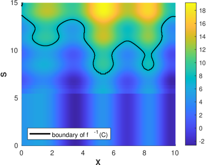
Figure 2: Representation of $f_{1}$ (right) and probability density function associated to $\mathds{P}_{S}$ (left). The black curve represents the contour of $\gamma(f)$.

The second test function is defined on $\mathds{X}=[-2;2]^{2}$ and $S=[-1;1]^{2}$ by

$$f_{2}\left((x_{1},x_{2}),\,(s_{1},s_{2})\right)=\frac{1}{2}\,c(x_{1},s_{1})+\frac{1}{2}\,c(x_{2},s_{2}),$$ (21)

with $c$ the “six-hump camel” function $c(x,s)=\left(4-2.1x^{2}+\frac{x^{4}}{3}\right)x^{2}+xs+(4s^{2}-4)s^{2}$ (Dixon and Szegö, 1978). We take $C=(-\infty;T]$ with $T=1.2$, $\alpha=0.15$ and $\mathds{P}_{S}$ the uniform distribution on $\mathds{S}$. The corresponding set $\Gamma(f_{2})$ is shown in Figure 3.

As a third test function $f_{3}$, we consider the Hartmann4 function, in the form of Picheny et al. (2013), defined on $\mathds{X}=[0;1]^{2}$ and $\mathds{S}=[0;1]^{2}$ equipped with the uniform distribution. We define $\alpha=0.6$ and $C=(-\infty,T]$, with $T=1.1$.

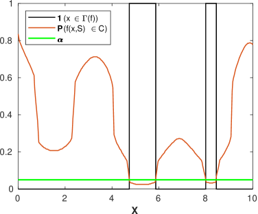
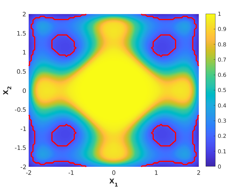
Figure 3: Representation of $x\mapsto\mathds{P}(\{s\in\mathds{S}\,:\,f(x,s)\in C\})$ and $\Gamma(f)$ for the artificial test functions $f_{1}$ (left) and $f_{2}$ (right).

5.2 Application to history matching

The objective of this application is to retrieve the set of plausible deterministic input variables of a numerical simulator, given real-life measurements. Such problem can be seen as a particular case of a “history matching” problem (see, e.g., Williamson et al., 2013). More precisely, we consider an uncertain Mogi model (Mogi, 1958), whose aim is to simulate the displacement at the surface of a volcano caused by an underground magma reservoir, while taking into account the mechanical property of the soil (Durrande and Le Riche, 2017).

Formally, the simulator can be seen as a function $v:\mathds{X}\times\mathds{S}\to\mathds{R}^{220}$, with inputs $(x_{1},x_{2},x_{3},x_{4},x_{5})\in\mathds{X}=[0,1]^{5}$ representing the normalized latitude, longitude, elevation, radius and overpressure of the magma source and $(s_{1},s_{2})\in\mathds{S}=[0,1]^{2}$ representing uncertain perturbations of the shear modulus and Poisson ratio of the material. The uncertain variables are assumed independent and identically distributed, following a Beta distribution with parameters $(2,2)$.

Given the real measurements $(y_{i})_{i\in\{1,\,...\,,220\}}$ and considering the mean absolute error $V(x,s)=\frac{1}{220}\sum_{i=1}^{220}|v_{i}(x,s)-y_{i}|$, our objective is to retrieve the set of plausible parameters for the Mogi model. More specifically, in this application, a vector of parameters $x\in\mathds{X}$ is considered to be “plausible” if it yields an error strictly less than $0.015$ with a probability larger than $0.1$. To exhibit the direct link between this history matching problem and the QSI framework, notice that it can be equivalently reformulated as the problem of estimating the set $\Gamma(V)$, with critical region $C=[0.015,+\infty)$ and $\alpha=0.9$.

5.3 Implementation details

We use for all the examples a GP prior with an unknown constant mean and an anisotropic Matérn covariance function. At each step of the algorithm, the parameters of the Gaussian prior are estimated using the restricted maximum likelihood (ReML) method (see, e.g., Stein, 1999), with the constraint that the regularity parameter $\upsilon$ of the kernel belongs to $\left\{\frac{1}{2},\frac{3}{2},\frac{5}{2},+\infty\right\}$, where the limit case $\upsilon\rightarrow+\infty$ corresponds to the Gaussian kernel.

Note that in what follows, all sampling are assumed to be without replacement. At each step, we first sample $n_{\mathds{S}}$ points according to $\mathds{P}_{S}$ as a discretization grid $\widetilde{\mathds{S}}$ of $\mathds{S}$. Then, a set of $n_{\mathds{X}}$ points is uniformly sampled in $\mathds{X}$ (with $n_{\mathds{X}}=500d_{\mathds{X}}$ in our experiments). For each of these points, we approximate the misclassification probability $\min(\pi_{n}(x),1-\pi_{n}(x))$ using Monte Carlo simulations of $\xi(x,\cdot)$ on $\widetilde{\mathds{S}}$ (with respect to $\mathds{P}_{n}$). Finally, a subset $\widetilde{\mathds{X}}$ is constructed from the point with the highest misclassification probability, and a sample of $n_{\pi}-1$ points drawn, according to the discrete probability distribution $p_{\mathds{X}}(x)\propto\min(\pi_{n}(x),1-\pi_{n}(x))$. This particular distribution is chosen to ensure that the elements of $\widetilde{\mathds{X}}$ are concentrated in the areas of $\mathds{X}$ where the probability of misclassification is high. This procedure gives us a product set $\widetilde{\mathds{X}}\times\widetilde{\mathds{S}}$, used to approximate the integrals involved in the QSI-SUR sampling criterion, as explained in Section 4.2.

The approximated sampling criterion is then optimized using an exhaustive search over a subset $\widetilde{\mathds{D}}\subset\widetilde{\mathds{X}}\times\widetilde{\mathds{S}}$ of candidate points, over which a Gauss-Hermite quadrature is used to approach the integrand (18). To construct this subset of candidate points, we evaluate the probability of misclassification $\min(p_{n}(x,s),1-p_{n}(x,s))$ of $\xi(x,s)\in C$, and, following the same idea as previously, keep the point with the highest misclassification probability and a random set of $n_{c}-1$ points drawn, according to the probability vector proportional to $\min(p_{n}(x,s),1-p_{n}(x,s))$ as $\widetilde{\mathds{D}}$.

We follow the rule of thumb which consists of taking an initial design of size $n_{0}$ equals to ten times the input dimension of the problem (Loeppky et al., 2009). The values of the simulation parameters used for the QSI-SUR implementation (and the comparative methods implementations, see supplementary material) are summarized in Table 1.

Test case	$\alpha$	$d_{\mathds{X}}+d_{\mathds{S}}$	$n_{0}$	$n_{\mathds{X}}$	$n_{\mathds{S}}$	$n_{\pi}$	$n_{c}$	$N$	$M$
$f_{1}$	$0.05$	$1+1$	20	500	100	15	200	15	250
$f_{2}$	$0.15$	$2+2$	40	1000	25	60	200	15	250
$f_{3}$	$0.60$	$2+2$	40	1000	25	60	200	15	250
“Volcano”	$0.90$	$5+2$	70	2500	75	20	200	15	250

Table 1: Summary of the simulation parameters used in the numerical experiments. Note that $\operatorname{card}(\widetilde{\mathds{X}}\times\widetilde{\mathds{S}})=n_{\pi}n_{\mathds{S}}=1500$ for all the examples (cf. Remark 4).

All the numerical experiments are carried out using Matlab R2022a and the STK toolbox (Bect et al., 2022).

Remark 4

Due to the expensive nature of the simulation of conditional GPs, the simulation parameters described in this section must be calibrated according to the computational budget at hand. In particular $n_{\pi}$ and $n_{\mathds{S}}$ must be chosen such that $\operatorname{card}(\widetilde{\mathds{X}}\times\widetilde{\mathds{S}})=n_{\pi}n_{\mathds{S}}$ is sufficiently low to accommodate a given computation time.

5.4 Results

We compare the results obtained with the proposed QSI-SUR sampling criterion with several other Bayesian methods. Due to the absence in the literature of strategies dealing with the exact problem considered in this work, we focus on methods that aim at approximating the set $\gamma(f)=\{(x,s)\in\mathds{X}\times\mathds{S}\,:\,f(x,s)\in C\}$. It is clear indeed that a perfect knowledge of $\gamma(f)$ implies a perfect knowledge of $\Gamma(f)$.

More precisely, we compare our results to those obtained with the misclassification probability criterion (see Section 3.1) and with the SUR criteria corresponding to the uncertainty measure (6) for the random set $\gamma(\xi)$. As a baseline method, we also include the results obtained with random sampling of the evaluation points. More details about the implementation of these methods can be found in the supplementary material. The different algorithms are repeated $100$ times on all the test cases, using different pseudo-maximin LHS as initial designs.

For performances evaluation, we compare the proportions of misclassified points obtained on a prediction grid composed of the product of a Sobol’ sequence of $2^{13}$ points in $\mathds{X}$ and the inversion (with respect to the cumulative distribution function of $\mathds{P}_{S}$) of a Sobol sequence of $2^{8}$ points in $[0,1]^{d_{\mathds{S}}}$. Considering that the Bayes-optimal estimator (11) is too expensive to compute on such a large grid (using heavy Gaussian sample paths simulations on the prediction grid), we use instead the estimator $\widehat{\Gamma}_{n}=\{x\in\mathds{X}\,:\,\mathds{E}_{n}(\tilde{\tau}(x))\leq\alpha\}$, where $\tilde{\tau}(x)$ is the approximation of $\tau(x)$ defined by average over the $2^{8}$ selected points of $\mathds{S}$.

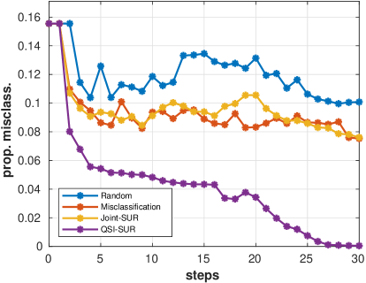
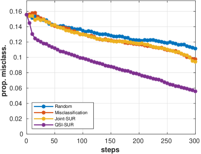
Figure 4: Median of the proportion of misclassified points vs. number of iterations, for 100 repetitions of the algorithms on the test functions $f_{1}$ (left) and $f_{2}$ (right).

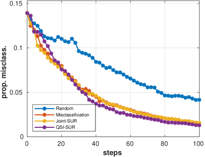
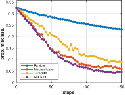
Figure 5: Median of the proportion of misclassified points vs. number of iterations, for 100 repetitions of the algorithms on the function $f_{3}$ (left) and the “volcano” test case (right).

From the results in Figure 4 and Figure 5, observe that the new sampling criteria tends to perform better on the QSI problem than the state-of-the-art methods focusing on the set $\gamma(f)$ in the joint space $\mathds{X}\times\mathds{S}$. Moreover, as illustrated in Figure 6 and in the complementary results of the supplementary material, the performances appear to never lag behind even in the worst cases.

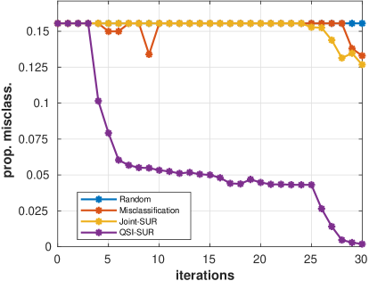
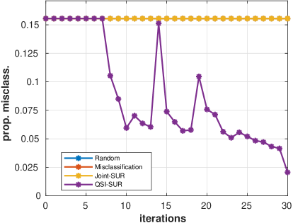
Figure 6: Quantiles of order $0.75$ (left) and $0.95$ (right) of the proportion of misclassified points vs. number of iterations, for 100 repetitions of the algorithms on the test function $f_{1}$.

These differences in performance can be explained, from a heuristic viewpoint, by the fact that, in the joint space $\mathds{X}\times\mathds{S}$, the new criterion tend to concentrate the evaluations around specific zones of $\gamma(f)$ which are particularly relevant for the approximation of $\Gamma(f)$. This phenomenon, related to the geometry of $\gamma(f)$, can be visualized on Figure 7. It is important to notice, however, that in some cases (illustrated here by the function $f_{3}$), the performances of the two kinds of methods are similar.

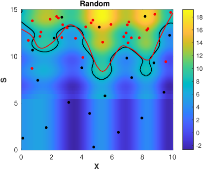
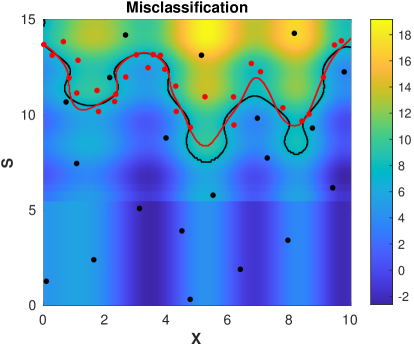
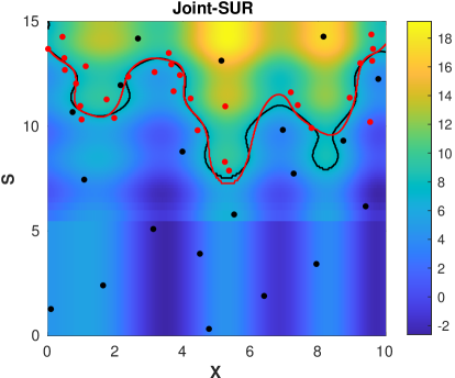
Figure 7: Examples of sequential designs (red dots) obtained after $n=30$ iterations on the function $f_{1}$, with the four sampling criteria. Black dots represent the initial design points, black curve the boundary of $\gamma(f)$, and red curve the boundary of $\gamma(\mu_{n})$.

From the results shown on Figure 8, we can observe that the performances of the misclassification-based and variance-based QSI-SUR criteria are similar. Such results are expected, given the fact that the variance and the entropy are both increasing transformation of the misclassification probability.

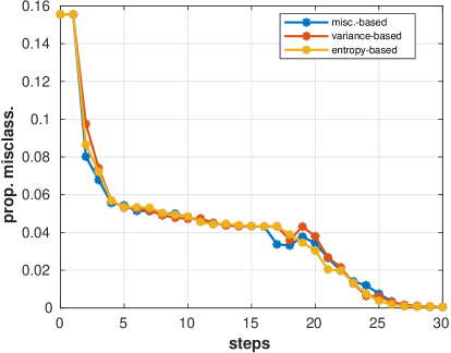
Figure 8: Median of the proportion of misclassified points vs. number of iterations, for 100 repetitions of different possible variants (in terms of $\mathcal{H}_{n}$) of the QSI-SUR method on the function $f_{1}$ (left) and the “volcano” test case (right).

More results regarding these numerical experiments can be found in the supplementary material, including figures similar to Figure 6 and Figure 8 for $f_{2}$, $f_{3}$ and “volcano”.

6 Conclusion

This article presents a SUR strategy for a particular set inversion problem, in a framework where a function admits deterministic and uncertain input variables, that we called Quantile Set Inversion (QSI). The practical interest of the proposed method is illustrated on several problems, on which methods that do not take advantage of the specificity of the QSI problem tend to be outperformed. However, this gain in performance comes at the cost of a high numerical complexity, in relation with the heavy use of conditioned Gaussian trajectory simulations. Future work will concentrate on making the method applicable to harder test problems (higher input dimensions, smaller probabilities, etc.) and on demonstrating its practical relevance to real-life problems.

Acknowledgements.

The authors are grateful to Valérie Cayol, Rodolphe Le Riche, Nicolas Durrande and Victor Picheny for sharing their R implementation of the Mogi model used in Section 5.

 

SUPPLEMENTARY MATERIAL

 

Appendix SM1 Proof of the expression of $\mathcal{H}_{n}$

Let us remark that

$$\Gamma(\xi)\Delta\widehat{\Gamma}_{n}=\left\{x\in\Gamma(\xi)\,:\,x\notin\widehat{\Gamma}_{n}\right\}\bigcup\left\{x\in\widehat{\Gamma}_{n}\,:\,x\notin\Gamma(\xi)\right\}.$$

In consequence, by defining the classifier $c_{n}(x)=\mathds{1}_{\widehat{\Gamma}_{n}}(x)$ and by Fubini theorem:

$$\mathds{E}_{n}\left[\lambda\left(\Gamma(\xi)\Delta\widehat{\Gamma}_{n}\right)\right] =\int_{\mathds{X}}\mathds{E}_{n}\left[\mathds{1}_{\Gamma(\xi)\Delta\widehat{\Gamma}_{n}}(x)\right]\,\mathrm{d}x$$

$$=\int_{\mathds{X}}\mathds{E}_{n}\left[\mathds{1}_{\{c_{n}=0\}}(x)\mathds{1}_{\Gamma}(\xi)(x)\right]$$

$$\qquad+\int_{\mathds{X}}\mathds{E}_{n}\left[\mathds{1}_{\{c_{n}=1\}}(x)\left(1-\mathds{1}_{\Gamma}(\xi)(x)\right)\right]\,\mathrm{d}x$$

$$=\int_{\mathds{X}}\mathds{1}_{\{c_{n}=0\}}(x)\,\pi_{n}(x)\,\mathrm{d}x+\int_{\mathds{X}}\mathds{1}_{\{c_{n}=1\}}(x)\left(1-\pi_{n}(x)\right)\,\mathrm{d}x.$$

It suffices to observe that, if $\widehat{\Gamma}_{n}=\left\{x\in\mathds{X}\,:\,\pi_{n}(x)>\frac{1}{2}\right\}$, then $c_{n}(x)=\mathds{1}_{\left\{\pi_{n}(x)>\frac{1}{2}\right\}}(x)$, and for all $x\in\mathds{X}$:

$$\mathds{1}_{\{c_{n}=0\}}(x)\pi_{n}(x)+ \mathds{1}_{\{c_{n}=1\}}(x)\left(1-\pi_{n}(x)\right)$$

$$=\mathds{1}_{\left\{\pi_{n}\leq\frac{1}{2}\right\}}(x)\pi_{n}(x)+\mathds{1}_{\left\{\pi_{n}>\frac{1}{2}\right\}}(x)\left(1-\pi_{n}(x)\right)$$

$$=\min\left(\pi_{n}(x),1-\pi_{n}(x)\right)$$

to obtain the simplified expression of $\mathcal{H}_{n}$.

Appendix SM2 Implementation details

In order to have coherent implementations of the comparatives methods regarding the QSI-SUR sampling criterion, adequate procedures are adopted. For clarity, we base the values of the simulation parameters involved on those used for the QSI-SUR implementation, of which we also recall the implementation.

In the following, all sampling are assumed to be without replacement.

• Random sampling: at each step, $f$ is evaluated at a random point sampled according to $\mathcal{U}(\mathds{X})\otimes\mathds{P}_{S}$.

• Misclassification: at each step, we sample $n_{\pi}\times n_{\mathds{S}}$ points in $\mathds{X}\times\mathds{S}$ according to $\mathcal{U}(\mathds{X})\otimes\mathds{P}_{S}$. We evaluate the function $f$ at the point with the highest misclassification probability $\min(p_{n}(x,s),1-p_{n}(x,s))$.

• Joint-SUR: at each step, we sample $n_{\mathds{X}}\times n_{\mathds{S}}$ points in $\mathds{X}\times\mathds{S}$ with respect to $\mathcal{U}(\mathds{X})\otimes\mathds{P}_{S}$. For each sampled point, we evaluate $p_{n}(x,s)$. The point with the highest probability of misclassification in $C$ is kept and $n_{\mathds{X}}\times n_{\mathds{S}}-1$ points are sampled according to $p_{\mathds{X}\times\mathds{S}}\propto\min(p_{n}(x,s),1-p_{n}(x,s))$, giving us the discretization grid $\widetilde{\mathds{D}}$. The joint-SUR criterion is then optimized using a search over a set of candidate points composed of the $n_{c}$ first sampled points of $\widetilde{\mathds{D}}$.

  Notice that, similarly to the QSI-SUR implementation, an importance sampling approximation based on the distribution $p_{\mathds{X}\times\mathds{S}}$ is used for the evaluation of the integral on $\mathds{X}\times\mathds{S}$ involved in the sampling criterion.

• QSI-SUR: at each step, we first sample $n_{\mathds{S}}$ points according to $\mathds{P}_{S}$ as discretization grid $\widetilde{\mathds{S}}$. We then uniformly sample a set of $n_{\mathds{X}}$ points in $\mathds{X}$. For each of those points, we approximate $\pi_{n}(x)$ using Monte Carlo simulation of $\xi(x,\cdot)$ on $\widetilde{\mathds{S}}$ (with respect to $\mathds{P}_{n}$). Finally, the point with the maximum misclassification probability is kept and we sample $n_{\pi}-1$ points according to $p_{\mathds{X}}(x)\propto\min(\pi_{n}(x),1-\pi_{n}(x))$. This procedure give us a product set $\widetilde{\mathds{X}}\times\widetilde{\mathds{S}}$, used to approximate the integrals involved in the QSI-SUR sampling criterion. The approximated sampling criterion is then optimized using an exhaustive search over a subset of the approximation grid $\widetilde{\mathds{D}}\subset\widetilde{\mathds{X}}\times\widetilde{\mathds{S}}$. To construct such subset of candidate points, we evaluate $p_{n}(x,s)$, and keep a random set of $n_{c}$ points composed of the point with the highest misclassification probability in $\gamma(\xi)$ and $n_{c}-1$ points sampled according to the probability vector proportional to $\min(p_{n}(x),1-p_{n}(x))$ as $\widetilde{\mathds{D}}$.

Appendix SM3 Complementary results for numerical experiments

SM3.1 Complementary results for the misclassification-based criterion

SM3.1.1 Artificial case $f_{1}$

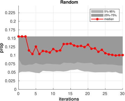
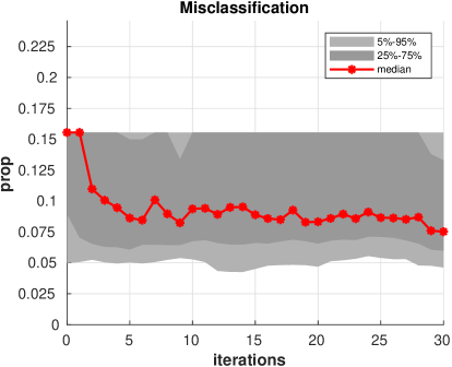
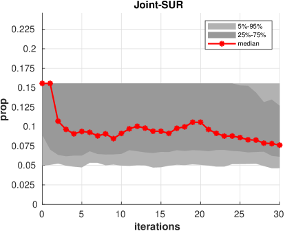
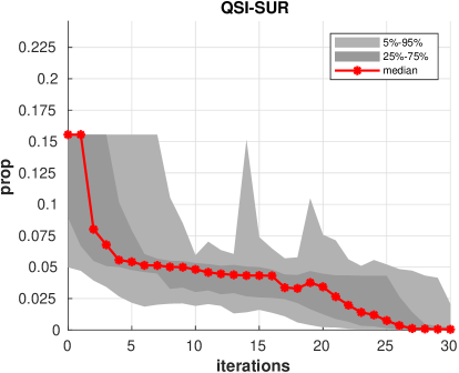
Figure SM1: Median and several quantiles of the proportion of misclassified points vs. number of iterations, for 100 repetitions of the algorithms on the test function $f_{1}$.

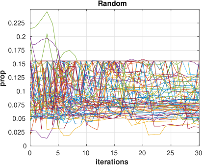
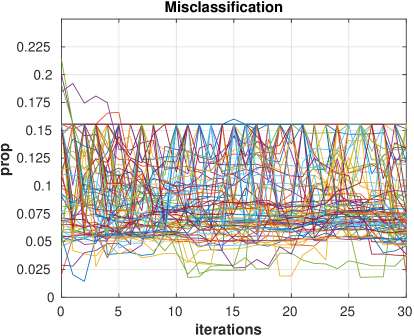
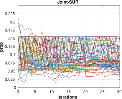
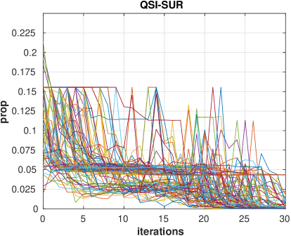
Figure SM2: Quantiles of level $0.75$ and $0.95$ for the proportion of misclassified points vs. number of iterations, for 100 repetitions of the algorithms on the test function $f_{1}$.

Figure SM3: Different trajectories of the proportion of misclassified points vs. number of iterations, for 100 repetitions of the algorithms on the test function $f_{1}$.

SM3.1.2 Artificial case $f_{2}$

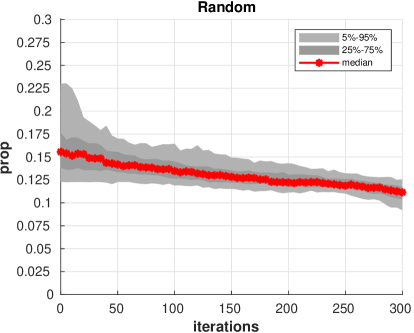
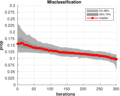
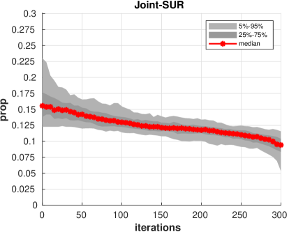
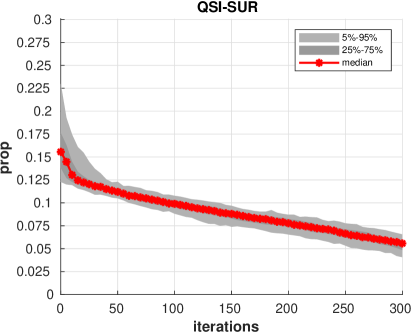
Figure SM4: Median and several quantiles of the proportion of misclassified points vs. number of iterations, for 100 repetitions of the algorithms on the test function $f_{2}$.

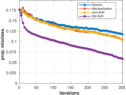
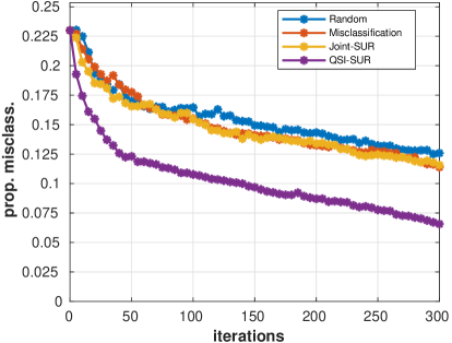
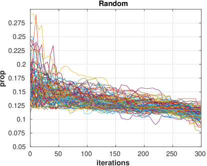
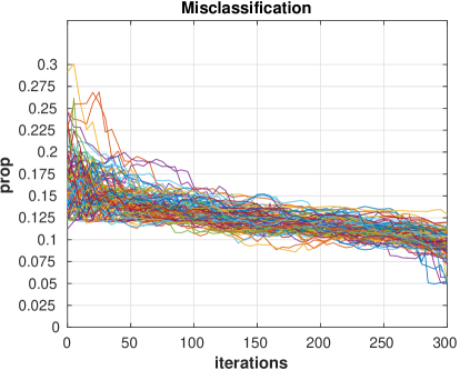
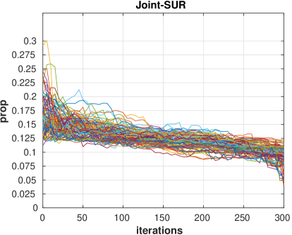
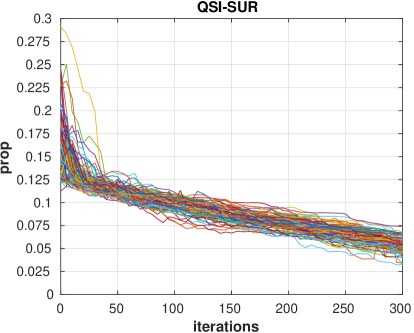
Figure SM5: Quantiles of level $0.75$ and $0.95$ for the proportion of misclassified points vs. number of iterations, for 100 repetitions of the algorithms on the test function $f_{2}$.

Figure SM6: Different trajectories of the proportion of misclassified points vs. number of iterations, for 100 repetitions of the algorithms on the test function $f_{2}$.

SM3.1.3 Artificial case $f_{3}$

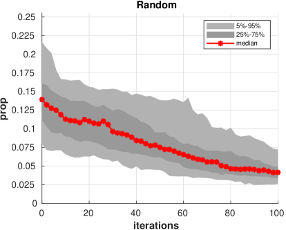
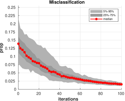
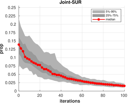
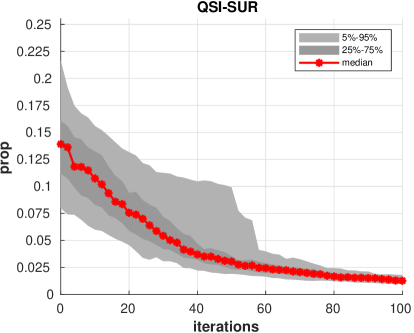
Figure SM7: Median and several quantiles of the proportion of misclassified points vs. number of iterations, for 100 repetitions of the algorithms on the test function $f_{3}$.

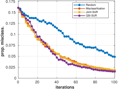
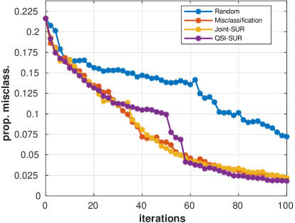
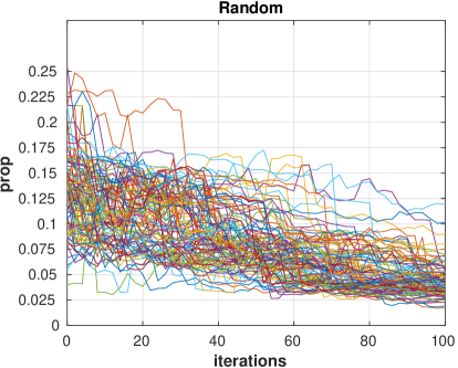
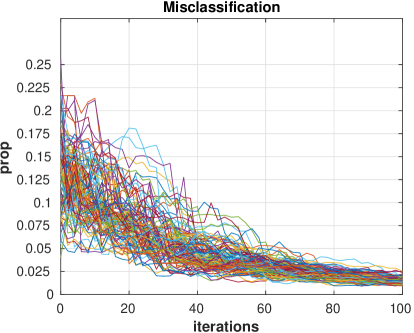
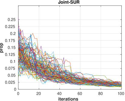
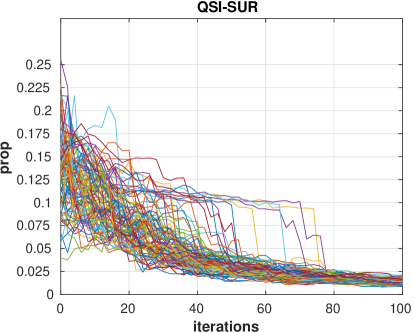
Figure SM8: Quantiles of level $0.75$ and $0.95$ for the proportion of misclassified points vs. number of iterations, for 100 repetitions of the algorithms on the test function $f_{3}$.

Figure SM9: Different trajectories of the proportion of misclassified points vs. number of iterations, for 100 repetitions of the algorithms on the test function $f_{3}$.

SM3.1.4 “Volcano” test case

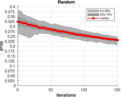
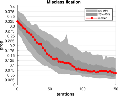
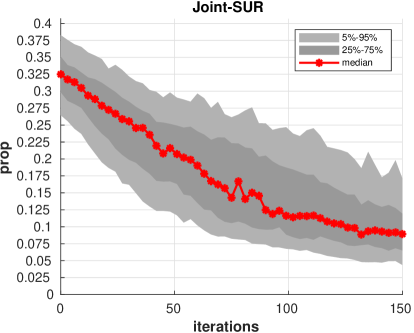
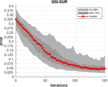
Figure SM10: Median and several quantiles of the proportion of misclassified points vs. number of iterations, for 100 repetitions of the algorithms on the “volcano” test case.

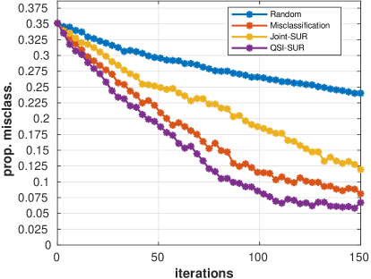
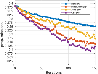
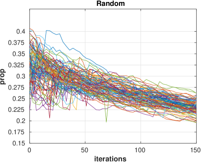
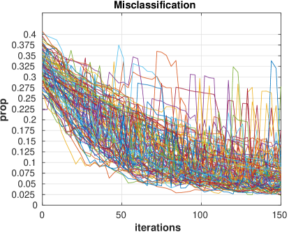
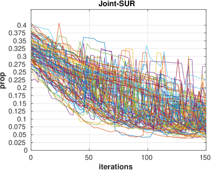
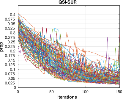
Figure SM11: Quantiles of level $0.75$ and $0.95$ for the proportion of misclassified points vs. number of iterations, for 100 repetitions of the algorithms on the “volcano” test case.

Figure SM12: Different trajectories of the proportion of misclassified points vs. number of iterations, for 100 repetitions of the algorithms on the “volcano” test case.

SM3.2 Comparison between variants of $\mathcal{H}_{n}$

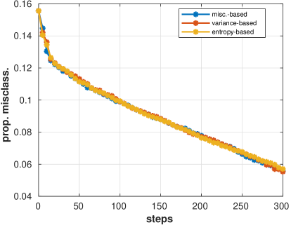
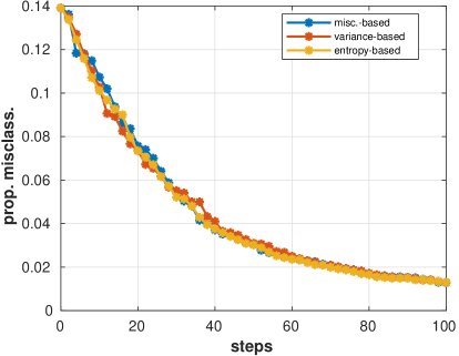
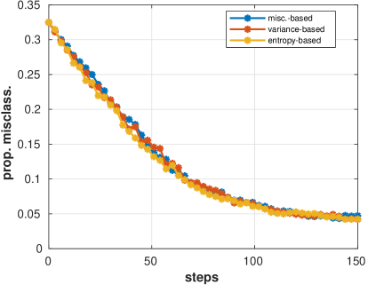
Figure SM13: Median of the proportion of misclassified points vs. number of iterations, for 100 repetitions of different possible variants (in terms of $\mathcal{H}_{n}$) of the QSI-SUR method on the function $f_{1}$, $f_{2}$, $f_{3}$ and the “volcano” test case (from left to right, top to bottom).

References

- Azzimonti et al. (2021) Azzimonti, D., D. Ginsbourger, C. Chevalier, J. Bect, and Y. Richet (2021). Adaptive design of experiments for conservative estimation of excursion sets. Technometrics 63(1), 13–26.
- Bect et al. (2019) Bect, J., F. Bachoc, and D. Ginsbourger (2019). A supermartingale approach to Gaussian process based sequential design of experiments. Bernoulli 25(4A), 2883–2919.
- Bect et al. (2012) Bect, J., D. Ginsbourger, L. Li, V. Picheny, and E. Vazquez (2012). Sequential design of computer experiments for the estimation of a probability of failure. Statistics and Computing 22, 773–793.
- Bect et al. (2022) Bect, J., E. Vazquez, et al. (2022). STK: a Small (Matlab/Octave) Toolbox for Kriging. Release 2.7.0.
- Bichon et al. (2008) Bichon, B. J., M. S. Eldred, L. P. Swiler, S. Mahadevan, and J. M. McFarland (2008). Efficient global reliability analysis for nonlinear implicit performance functions. AIAA Journal 46(10), 2459–2468.
- Branin and Hoo (1972) Branin, F. H. and S. K. Hoo (1972). A method for finding multiple extrema of a function of n variables. In F. A. Lootsma (Ed.), Numerical methods of Nonlinear Optimization, pp. 231–237. Academic Press.
- Bryan et al. (2005) Bryan, B., R. C. Nichol, C. R. Genovese, J. Schneider, C. J. Miller, and L. Wasserman (2005). Active learning for identifying function threshold boundaries. In Y. Weiss, B. Schölkopf, and J. Platt (Eds.), Advances in Neural Information Processing Systems, Volume 18. MIT Press.
- Chevalier (2013) Chevalier, C. (2013). Fast uncertainty reduction strategies relying on Gaussian process models. Ph. D. thesis, University of Bern.
- Chevalier et al. (2014) Chevalier, C., J. Bect, D. Ginsbourger, E. Vazquez, V. Picheny, and Y. Richet (2014). Fast parallel kriging-based stepwise uncertainty reduction with application to the identification of an excursion set. Technometrics 56(4), 455–465.
- Chevalier et al. (2013) Chevalier, C., D. Ginsbourger, J. Bect, and I. Molchanov (2013). Estimating and quantifying uncertainties on level sets using the Vorob’ev expectation and deviation with Gaussian process models. In D. Uciński, A. C. Atkinson, and M. Patan (Eds.), mODa 10 – Advances in Model-Oriented Design and Analysis, pp. 35–43. Springer.
- Dixon and Szegö (1978) Dixon, L. and G. P. Szegö (1978). The global optimization problem: an introduction. In L. C. W. Dixon and G. P. Szegö (Eds.), Towards Global Optimization 2. North Holland.
- Duhamel et al. (2023) Duhamel, C., C. Helbert, M. Munoz Zuniga, C. Prieur, and D. Sinoquet (2023). A SUR version of the Bichon criterion for excursion set estimation. Statistics and Computing 33, Article number: 41.
- Durrande and Le Riche (2017) Durrande, N. and R. Le Riche (2017). Introduction to Gaussian Process surrogate models. HAL cel-01618068. Lecture notes, 4th MDIS-Form@ter workshop, October 16–20, 2017, Besse en Chandesse, France.
- Echard et al. (2011) Echard, B., N. Gayton, and M. Lemaire (2011). AK-MCS: An active learning reliability method combining Kriging and Monte Carlo Simulation. Structural Safety 33(2), 145–154.
- El Amri et al. (2023) El Amri, R., C. Helbert, M. Munoz Zuniga, C. Prieur, and D. Sinoquet (2023). Feasible set estimation under functional uncertainty by Gaussian Process modelling. HAL preprint hal-02986558v3.
- Graf and Luschgy (2000) Graf, S. and H. Luschgy (2000). Foundations of Quantization for Probability Distributions. Lecture Notes in Mathematics. Springer.
- Jaulin and Walter (1993) Jaulin, L. and E. Walter (1993). Set inversion via interval analysis for nonlinear bounded-error estimation. Automatica 29(4), 1053–1064.
- Loeppky et al. (2009) Loeppky, J. L., J. Sacks, and W. J. Welch (2009). Choosing the sample size of a computer experiment: A practical guide. Technometrics 51(4), 366–376.
- Marques et al. (2018) Marques, A., R. Lam, and K. Willcox (2018). Contour location via entropy reduction leveraging multiple information sources. In Advances in Neural Information Processing Systems 31 (NeurIPS 2018), pp. 1–11.
- Marrel et al. (2022) Marrel, A., B. Iooss, and V. Chabridon (2022). The ICSCREAM Methodology: Identification of Penalizing Configurations in Computer Experiments Using Screening and Metamodel—Applications in Thermal Hydraulics. Nuclear Science and Engineering 196(3), 301–321.
- Mogi (1958) Mogi, K. (1958). Relations between the eruptions of various volcanoes and the deformations of the ground surfaces around them. Bulletin of the Earthquake Research Institute 36, 99–134.
- Molchanov (1991) Molchanov, I. S. (1991). Empirical estimation of distribution quantiles of random closed sets. Theory of Probability & Its Applications 35(3), 594–600.
- Picheny et al. (2010) Picheny, V., D. Ginsbourger, O. Roustant, R. T. Haftka, and N.-H. Kim (2010). Adaptive designs of experiments for accurate approximation of a target region. Journal of Mechanical Design 132(7), 071008 (9 pages).
- Picheny et al. (2013) Picheny, V., T. Wagner, and D. Ginsbourger (2013). A benchmark of kriging-based infill criteria for noisy optimization. Structural and Multidisciplinary Optimization 48(3), 607–626.
- Ranjan et al. (2008) Ranjan, P., D. Bingham, and G. Michailidis (2008). Sequential experiment design for contour estimation from complex computer codes. Technometrics 50(4), 527–541.
- Rasmussen and Williams (2006) Rasmussen, C. E. and C. K. I. Williams (2006). Gaussian Processes for Machine Learning. MIT Press.
- Richet and Bacchi (2019) Richet, Y. and V. Bacchi (2019). Inversion algorithm for civil flood defense optimization: Application to two-dimensional numerical model of the Garonne river in france. Frontiers in Environmental Science 7(160), 1–16.
- Santner et al. (2019) Santner, T. J., B. J. Williams, and W. I. Notz (2019). The Design and Analysis of Computer Experiments. Springer Series in Statistics. Springer.
- Sire (2022) Sire, C. (2022). Robust inversion under uncertaint for flooding risk analysis. Talk given at the SIAM Conference on Uncertainty Quantification (UQ22), MS10, April 12, Atlanta.
- Stein (1999) Stein, M. L. (1999). Interpolation of spatial data: some theory for kriging. Springer.
- Vazquez and Bect (2009) Vazquez, E. and J. Bect (2009). A sequential Bayesian algorithm to estimate a probability of failure. IFAC Proceedings Volumes 42(10), 546–550.
- Villemonteix et al. (2009) Villemonteix, J., E. Vazquez, and E. Walter (2009). An informational approach to the global optimization of expensive-to-evaluate functions. Journal of Global Optimization 44, 509–534.
- Williamson et al. (2013) Williamson, D., M. Goldstein, L. Allison, A. Blaker, P. Challenor, L. Jackson, and K. Yamazaki (2013). History matching for exploring and reducing climate model parameter space using observations and a large perturbed physics ensemble. Climate Dynamics 41, 1703–1729.