Thermal Simulation of Millimetre Wave Ablation of Geological Materials

Abstract

This work is concerned with the numerical simulation of ablation of geological materials using a millimetre wave source. To this end, a new mathematical model is developed for a thermal approach to the problem, allowing for large scale simulations, whilst being able to include the strong temperature dependence of material parameters to ensure accurate modelling of power input into the rock. The model presented is implemented within an adaptive meshing framework, such that resolution can be placed where needed, for example at the borehole wall, to further improve the computational efficiency of large scale simulations. This approach allows for both the heating of the rock, and the removal of evaporated material, allowing rate of penetration and the shape of the resulting borehole to be quantified. The model is validated against experimental results, which indicates that the approach can accurately predict temperatures, and temperature gradients within the rock. The validated model is then exercised to obtain initial results demonstrating its capabilities for simulating the millimetre wave drilling process. The effects of the conditions at the surface of the rock are investigated, highlighting the importance of understanding the physical processes which occur between the wave guide and the rock. Additionally, the absorptivity of the rock, and the impact this has on the evaporation behaviour is considered. Simulations are carried out both for isotropic rock, and also for a multi-strata configuration. It is found that strata between similar rock types, such as granite and basalt, absorptive properties pose little problem for uniform drilling. However, larger variations in material parameters are shown to have strong implications on the evaporation behaviour of the wellbore, and hence the resulting structure.

I Introduction

The use of electromagnetic (EM) waves as a technology for drilling has been considered since the early days of laser-driven applications Oglesby et al. (2014). In particular, this process could allow for more efficient drilling through materials which are problematic for conventional drill bits, such as igneous rock. However, efficiency issues with laser sources, and the energy input requirements for melting and vaporising rock, limited development of EM drilling technology. Oglesby Oglesby et al. (2014) addressed efficiency concerns by using a gyrotron, instead of a laser, which produces a millimetre wave (MMW) EM signal, with frequency in the range 30-300 GHz and for which efficiency of commercially available units can exceed 50% Kasugai et al. (2008).

Through the use of MMW drilling technology, and the advent of commercially available high-power gyrotrons, Oglesby Oglesby et al. (2014) identifies several benefits over conventional methods. For use in wellbore drilling, using MMWs is expected to correspond to a linear increase in drilling cost with respect to depth, whilst for conventional methods, cost increases exponentially with depth. Additionally, the technology is applicable to rocks of all hardness, and high-temperature material is not a limiting factor in potential drill depth Raymond (1999); Woskov and Cohn (2008). Related to this is the fact that there is enhanced reliability and durability with a gyrotron source, due to the fact that it does not come in contact with the rock itself. It is also possible that the process can be controlled such that the molten material forms a vitrified liner to a wellbore during the drilling process. Finally, in comparison to other EM sources, MMW propagation through a dusty or particulate medium is relatively efficient, which reduces requirements for control of the evaporated material down a wellbore. These advantages suggest MMWs could be a valuable technology for deep drilling in igneous rock environments, with applications such as geothermal energy generation and nuclear waste entombment. The former of these options is of particular interest since it allows energy to be obtained through an Enhanced Geothermal Systems (EGS) approach, requiring the drilling of hot rock with very low natural permeability or fluid saturationTester et al. (2006), which are conditions unfavourable for conventional technology. Successful drilling within these conditions could allow for widespread use of geothermal energy McClure and Horne (2014).

In order to utilise MMWs for drilling to the depths required for geothermal energy or other applications, understanding the evaporation process, and how it can be controlled, is essential. The initial cost of a high-powered gyrotron limits the number of experimental studies into these techniques, though Woskov and co-authors have run a series of laboratory-scale experiments on a variety of rocks, including basalt, granite, limestone and sandstone Woskov and Cohn (2009); Woskov and Michael (2012); Woskov, Einstein, and Oglesby (2013, 2014); Oglesby et al. (2014); Woskov and Cohn (2008). Even for these experiments, in many cases there was insufficient power used to achieve full vaporisation, though the capabilities of the process to heat and melt these materials could be investigated. Due to these experimental challenges, and the lack of information that will be available from down-well situations, numerical modelling allows for further insight to understand and guide experimental work.

In this work, a thermal model of the drilling process is developed, allowing for simulation of the MMW evaporation process over long length and time scales. This model allows for the change in material properties of the rock over the temperature ranges of interest, ambient conditions to evaporation, to be considered. Particular focus is placed on granite and basalt since these rocks are typically suitable for EGS technology, due to the difficulties in using conventional drilling techniques in these rocks Tester et al. (2006); McClure and Horne (2014). In addition to the temperature-dependent thermodynamic properties of these rocks, the dependence on MMW absorption is also considered, which effectively transitions from volumetric to surface heating of the material with increasing temperature.

The rest of this paper is laid out as follows; section II describes the mathematical and physical formulation of the model, including material parameters of the rocks considered, and the numerical methods for simulating the MMW drilling process are given in section III. Section IV provides a validation study, demonstrating the ability of the numerical model to reproduce experimental measurements. Section V considers further evaluation of the approach for a single material, investigating changes in properties of the rock, whilst section VI introduces multiple strata, considering the effects of two layers of material, with an angled interface between them. Finally, conclusions and further work are described in section VII.

II Mathematical formulation

The overall problem of rock ablation through MMW drilling is complex, and involves multiple time and length scales. The full process involves phase change from solid to molten rock, and subsequently to vapour, at which point gas flow (typically an inert gas) carries vaporised material away from the bottom of the wellbore. Additionally, molten rock will flow under the induced thermal gradients and reflection and scattering of the MMW source makes modelling energy input into the rock a complex process. Finally, the physical and absorptive properties of rock are strongly, and non-linearly, temperature dependent.

In order to simulate this process at large scales, such that rate of penetration can be measured, potentially thorough multiple material strata, this work assumes that the overall drilling process is governed by a thermal model. Gas flow occurs on a time scale too short for this scale, and can be considered a boundary condition, whilst material flow is assumed to occur over length scales too small to allow for efficient large scale simulations. This reduces the complexity of the system of equations required to describe the MMW drilling process, however the material properties cannot be simplified in such a manner. The non-linear thermal treatment of the rock is still included in the model presented here. Scattering of the MMW source is not directly considered in this work, but rather, a simplified energy input is employed. However, since energy input occurs through a source term, the model presented here is compatible with more advanced techniques for determining the MMW source behaviour.

The aim of this model is to enable the simulation of the evaporation process over long time scales (10s of seconds upwards) and large length scales. In order to achieve this with reasonable computational efficiency, it is assumed that material transport effects are negligible, and pressure is constant. Under these assumptions, the system reduces to a single thermal equation,

$$\rho(T)c_{p}(T)\frac{\partial T}{\partial t}=\nabla\cdot\left(\kappa(T)\nabla T\right)+\dot{q},$$ (1)

where, $T$ is temperature, $\rho$ density, $c_{p}$ specific heat at constant pressure, $\kappa$ thermal conductivity and $\dot{q}$ is a heat transfer term.

This final term comprises the heat input from the MMW source, as well as contributions from radiation and convection, and is given by

$$\dot{q}=\dot{Q}-\varepsilon\sigma\left(T^{4}-T^{4}_{0}\right)-h\left(T-T_{0}\right)$$ (2)

where $\dot{Q}$ is the input from the MMW source, $T_{0}$ is the temperature above the surface, $\varepsilon$ is the emissivity of the surface, $\sigma$ is the Stefan-Boltzmann constant and $h$ is the air convection coefficient.

The input, $\dot{Q}$, is given by

$$\dot{Q}=P({\bf x})\alpha_{\lambda}(T)\exp\left(-\alpha_{\lambda}(T)(z_{0}-z)\right)$$ (3)

where $P({\bf x})$ is the power incident on the surface, $z_{0}=z_{0}(x,y,t)$ is the height of the surface, and $\alpha_{\lambda}(T)$ is the absorption coefficient of the medium, which may itself depend on temperature. The incident power is dependent on both the MMW profile, which, in practice, emerges from a wave guide above the material surface, and also on the distance to this surface. In this work, it is assumed that the source profile is Gaussian, and that it is aligned with the $z$-axis, giving an incident surface power of

$$P=I_{0}\left(\frac{\omega_{0}}{\omega(z_{0}-z)}\right)^{2}\exp\left(\frac{-2r^{2}}{\omega(z_{0}-z)^{2}}\right)$$ (4)

where $I_{0}$ is the peak intensity, $\omega_{0}$ is the wave guide radius, $\omega(z_{0}-z)$ is the radius of the beam at which intensity is given by $I=I_{0}e^{-2}$ and, for a wave guide centred on $(x_{0},y_{0})$, $r^{2}=(x-x_{0})^{2}+(y-y_{0})^{2}$. The peak intensity is given by

$$I_{0}=\frac{2P_{0}}{\pi\omega^{2}}$$ (5)

where $P_{0}$ is the peak incident power, and $\omega(z_{0}-z)$ is computed through

$$\omega(z_{0}-z)=\omega_{0}\sqrt{1+\left(\frac{z_{0}-z}{z_{R}}\right)^{2}}$$ (6)

where $z_{R}$ is the Rayleigh range, which is related to the source wavelength, $\lambda$, through

$$z_{R}=\frac{\pi\omega^{2}_{0}n}{\lambda}$$ (7)

and in this work, $n=1$ is used. This approach, though relatively simple, does allow the stand-off distance between the surface and the wave guide to be considered, allowing some dispersion, and absorption from the gas, over this distance.

Here, it is noted that experimental tests have shown that the MMW source is capable of breaking down the air between wave guide and surface, generating a plasma Oglesby et al. (2014); Woskov and Cohn (2008). This is substantially more absorptive than unionised air, and can reduce the incident power on the surface by three orders of magnitude. However, in practice, inert gas flow will be used to prevent plasma formation, hence these effects are not incorporated within the model presented here; it is assumed that all absorption from this gas is based on equilibrium conditions.

The thermal model, given by equation (1), is augmented with a material removal model, dealing with the case in which the evaporation temperature of rock is exceeded. This technique assumes that once material has evaporated, it is entrained within gas flow at the surface, and thus will not condense again at, or close to, the evaporation front. Within the overall model, this behaviour is achieved by altering the properties of any region of the computational domain which reaches, or exceeds, the evaporation temperature of the rock. Once this condition has been reached, the material properties are then altered to be that of the surrounding gas. To implement this process, and additional scalar variable is used to describe the material in each cell, e.g. a rock (of which there may be multiple types) or gas.

Simulation of MMW drilling requires properties for rock to be understood from ambient conditions up to their vaporisation temperature (in excess of 3,000 K). Over these ranges, density, thermal conductivity, specific heat and absorptivity all vary substantially. For lower temperature ranges, up to around 1,300 K, these properties are well studied, see, for example, Heuze Heuze (1983), Hartlieb et al. Hartlieb et al. (2016), Branscome Branscome (2006) and Waples and Waples Waples and Waples (2004). However, above these ranges, properties are not well known, in part due to the high experimental cost for such investigations. For many thermal properties, Oglesby has found that using simple linear or constant extrapolations from known behaviour is typically sufficient to give reasonable high-temperature behaviour Oglesby et al. (2014). Such behaviour can be augmented where necessary through studies on magma, undertaken by the United States Geological Serviced, detailed by Robertson Robertson (1988).

Density of geological materials as a function of temperature may be known for temperatures below $\sim 1000$ K but above this, few measurements exist. In this work, density is given by Oglesby et al. (2014)

$$\rho=a_{\rho}(T-273.15)+b_{\rho}$$ (8)

where $a_{\rho}$ and $b_{\rho}$ are constants. This equation holds up until a cut-off value (determined by the limits of experimental measurements), after which a constant extrapolation is used, to ensure density values do not drop unphysically low.

Thermal conductivity is treated in a similar manner, in this case, however, two possible functional forms exist Oglesby et al. (2014);

$$\kappa=\frac{1}{a_{\kappa}+b_{\kappa}(T-273.15)}$$ (9)

or

$$\kappa=c_{\kappa}(T-273.15)^{2}+d_{\kappa}(T-273.15)+e_{\kappa}$$ (10)

with constant parameters, $a_{\kappa}$, $b_{\kappa}$, $c_{\kappa}$, $d_{\kappa}$ and $e_{\kappa}$. As with density, above a threshold, thermal conductivity is treated as constant.

Specific heat is treated slightly different from the other parameters, in that it contains a contribution from experimental measurements, and an additional contribution over phase change ranges to deal with latent heating effects. For the materials considered in this work, approximations to experimental measurements use a quadratic expression up to a threshold value, and subsequently a linear fit Oglesby et al. (2014). This gives a general form

$$c_{p}=\begin{cases}a_{c}(T-273.15)^{2}+b_{c}(T-273.15)+c_{c}&T\leq T_{c}\\ d_{c}(T-273.15)+e_{c}&T>T_{c}\end{cases}$$ (11)

In order to incorporate latent heat behaviour into the model, the approach of Yang et al. Yang et al. (2010) and Oglesby Oglesby et al. (2014) is followed. Here, the latent heat of fusion, $\xi_{f}$, is linearly distributed between solidus and liquidus temperatures ($T_{s}$ and $T_{l}$ respectively), and a similar treatment is used for the latent heat of evaporation, $\xi_{v}$. In this latter case, the temperature range over which evaporation occurs is not known for rocks, and an approximation, to distribute the latent heat effects over a 270 K temperature range, starting from evaporation temperature, is used. The overall specific heat is then the sum of these two contributions.

The absorptivity of a material is dependent on the permittivity, $\epsilon$, permeability, $\mu$, and electrical conductivity, $\gamma$, of the material itself, and also the frequency of the source, $\omega$. In practice, this can be computed through

$$\alpha_{\lambda}=2\omega\sqrt{\frac{\epsilon\mu}{2}}\left[\sqrt{1+\left(\frac{\gamma}{\epsilon\omega}\right)^{2}}-1\right]^{\frac{1}{2}}$$ (12)

however, the material properties for rocks are not necessarily known. As a result, the absorptivity is typically experimentally measured, and assumed to be piece-wise constant, potentially jumping between solid and liquid phases Oglesby et al. (2014); Woskov and Michael (2012).

II.1 Treatment of quartz $\alpha$-$\beta$ transition

Quartz content of a geological material can have an effect on its thermal properties since it exhibits an $\alpha$-$\beta$ transition at around 845 K Le Chatelier (1890); Robertson (1988); Dolino (1990); Hartlieb et al. (2016), and this subsequently alters the specific heat of the quartz, and hence the underlying rock Navrotsky (2018). In this work, we consider basalt, which has a low quartz content, and thus these effects are negligible, and granite, which has a much higher quartz content. Here, care has to be taken, both when attempting to obtain functional fits to experimental data for specific heat of a granite when temperature crosses this transition region, and also in incorporating these effects within the numerical model. Figure 1 compares two functional fits to experimental data for granite, one in which the values measured over the phase transition have not been accounted for, and a second showing the phase transition removed. It is clear that by removing the phase transition effects from this functional fit, the overall error in approximating the specific heat can be reduced. However, in order to model the behaviour within this region, specific heat is then increased within the transmission region, using a similar technique as is used to incorporate latent heat effects.

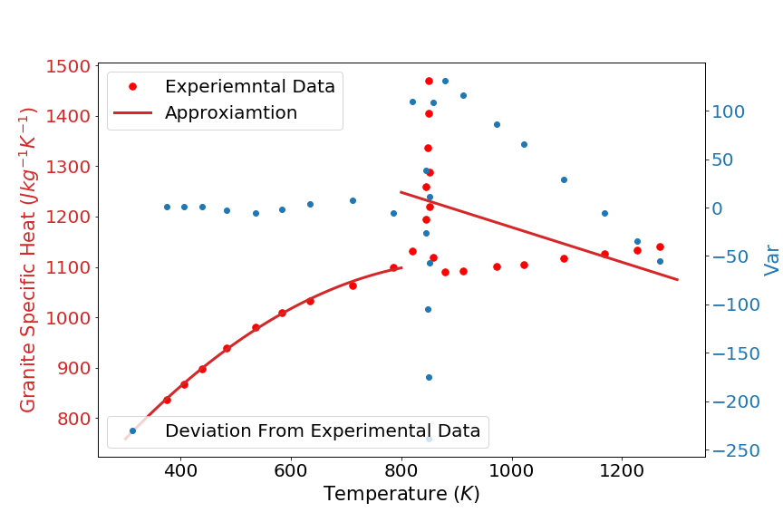
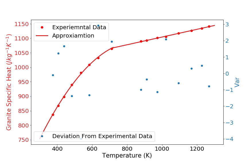
Figure 1: Comparison of linear approximations to specific heat data both with (top) and without (bottom) taking the $\alpha$-$\beta$ phase transition of quartz into account. Red points show the experimental data, red lines show the approximation to this data, and the relative error to measured points is shown by the blue dots. By removing the phase transition behaviour from the approximation, it is clear that accuracy increases, thought this requires an additional treatment to get the correct specific heat within this transition region.

III Numerical approach

The numerical techniques used to solve the model formulated in section II have been designed to deal with the length and time scales of the problems of interest. The absorptivity of materials such as basalt and granite, described by equation (3), are such that a significant portion of the incident energy is absorbed over a short length scale when compared to the diameter of the incident beam. As a result, there is a strong temperature gradient at the evaporation front, which requires suitable computational resolution to be modelled accurately. To achieve this desired resolution, whilst retaining computational efficiency, a finite volume formulation is used for solving equation (1), upon which hierarchical adaptive mesh refinement (refining in both space and time) can be implemented. In addition to solving for the temperature profile, two additional variables are updated; the material identifier required for the material removal model, and the vertical depth beneath the surface of each position within the computational domain. This latter variable is used in computing the MMW beam absorption in equation (3).

In order to solve equation (1), and to update these additional properties, a three-step process is implemented:

1. Using the data at the current time $t=t^{n}$, compute the power incident upon the current surface, and use this to update the temperature to time $t^{n+1}=t^{n}+\Delta t$ for a given time step $\Delta t$. To do this, equation (1) is cast into canonical form

   $$\left(A\alpha+B\nabla\cdot\beta\nabla\right)T=f$$ (13)

   where $A$ and $B$ are scalars, and $\alpha$, $\beta$ and $f$ are scalar fields. The solution is obtained using the biconjugate gradient stabilised method (BiCGSTAB) Van der Vorst (1992).

2. For any volumes in the computational domain with $T>T_{v}$, set the properties in this cell to be those of the surrounding gas. It is assumed that there is a gas flow over the surface of the material which removes vaporised and particulate matter, for which the surface treatment described in section III.2 is used.

3. Use the interface between the geological material and the surrounding gas to recompute the depth beneath the surface, using the techniques described in section III.1.

III.1 Determining surface height

In order to correctly prescribe the volumetric heating term of equation (3), the depth beneath surface is required. The surface, $z_{0}$, evolves with time through material evaporation, and thus an additional technique is required to track the depth. In this work, a signed distance function, $\phi$, is used, which satisfies

$$\left|\frac{\partial\phi}{\partial z}\right|=1$$ (14)

and the zero contour, $\phi({\bf x})=0$, describes the current surface of the rock.

In order to compute the signed distance function, a fast sweeping algorithm is used Zhao (2005). This requires knowledge of the current location of the interface; within this work, the it is known whether a computational cell is either rock (molten or solid) or surrounding gas, hence the interface can be set to be at the cell boundary between the transition from rock to gas.

III.2 Surface heat losses

One of the key challenges in ensuring accurate melt treatments, and for validating the methods presented in this work, is the treatment of the surface conditions, which are not well studied for geological materials under temperatures such as those achieved through a MMW source. The convective coefficient, $h$, depends not only on the temperature of the underlying material, but also on the conditions at the surface, and will vary depending on the level of gas flow, with a potential range of $h\in[25,250]$ W/m² K. Similarly, the surface losses are affected by the temperature of the material above the surface ($T_{0}$ in equation (2)). Even with air flow over the surface, the high temperatures beneath the MMW source will cause local temperature to exceed ambient conditions.

In order to ascertain suitable conditions for surface heat losses, several cases were computationally considered with a granite substrate, varying the convection coefficient (both for solid and molten material), as well as $T_{0}$. It is noted that it is not computationally efficient to solve the heat loss problem at the surface; this requires considering the gas flow, and occurs at time scales substantially shorter than those of material evaporation, and would hence have a detrimental effect on computational efficiency. It was found that assuming a surface temperature of

$$T_{0}=\mathrm{min}\left(T_{\mathrm{initial}},0.86T_{\mathrm{surface}}\right)$$ (15)

was a straightforward, yet accurate, technique to deal with these effects, where $T_{\mathrm{surface}}$ is the temperature of the material at the surface. It is noted that this approach did not consider the possible increase in the convective heat transfer coefficient at higher temperatures, though improving this aspect of the model would require further experimental study.

III.3 Adaptive mesh refinement

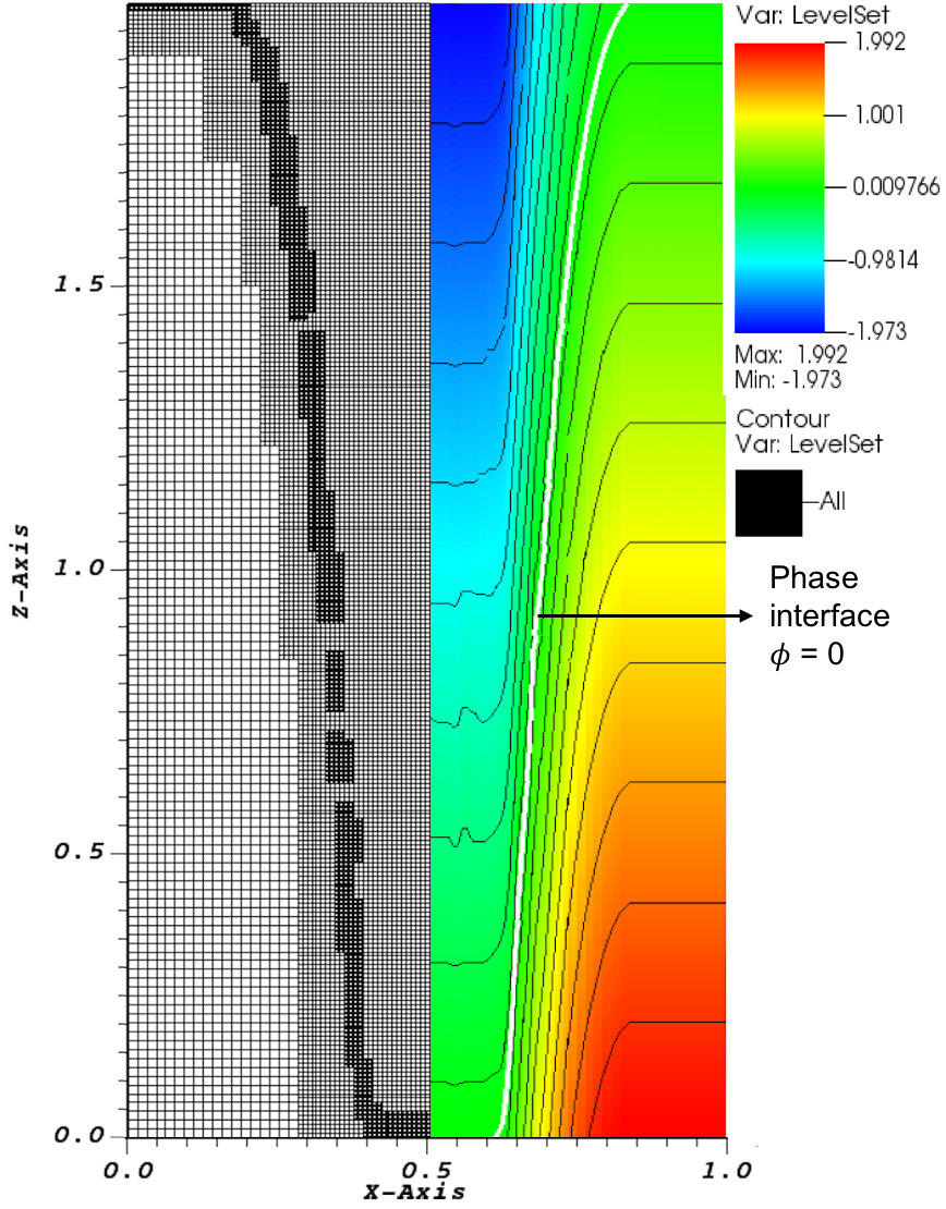
Figure 2: Demonstration of the application of AMR and of the level set function for recording material depth. AMR is applied based on temperature and material interface parameters, allowing the regions of strongest temperature gradient to be captured at the highest resolution. It is noted that the contours within the wellbore do suffer from visualisation artefacts caused by the automatic interpolation of the contour location.

The numerical methodology described in this section is inherently suitable for hierarchical adaptive mesh refinement (AMR) Bell et al. (1994). This technique allows for regions of the domain to be both refined in space and in time, hence regions of the computational domain far from the energy source can be evolved with a larger time step than those refined regions with high temperatures and strong temperature gradients. In this work, two thresholds are used to govern where AMR places the additional refinement, based on the governing processes which lead to material removal; temperature thresholds, e.g. $T>T_{m}$, and the location of the material interface. It is noted that these two regions will typically coincide for the ablation of geological materials, but by refining the material interface, it is ensured that this region is represented accurately, even when it is no longer being directly heated, and thus allowing for accurate quantification of the wellbore shape.

Figure 2 shows a typical mesh distribution, with the level set function also plotted to demonstrate how the additional resolution follows the material interface. The efficiency of a simulation using AMR depends heavily on the proportion of the domain covered by the refined mesh, but even in cases with a wellbore occupying a large portion of the computational domain, simulations are demonstrably more efficient with mesh refinement. Sample results, which show the improvements in computational run time, are shown in table 1. Comparisons are made between simulations with the same finest resolution ($32\times 32\times 64$ or $64\times 64\times 128$ on a single CPU), with and without AMR. The benefits of mesh refinement are clear; using two levels of mesh refinement, using two levels of AMR reduces run times by about 50%. In these cases, greater gains are not seen due to the proportion of the domain occupied by the wellbore surface, which is always refined. Moving to larger geometries, however, greater gains could be made, where the wellbore only needs refinement where there is power input, and thus these results can be thought of as the minimum gains available from AMR.

Resolution	Simulation	Resolution	Simulation
(cells)	time (s)	(cells)	time (s)
$64\times 64\times 128$	9423	$32\times 32\times 64$	1311
$32\times 32\times 64$		$16\times 16\times 32$
1 AMR level	7509	1 AMR level	854
$16\times 16\times 32$		$8\times 8\times 16$
2 AMR levels	5762	2 AMR levels	599

Table 1: Comparison of simulation times with and without AMR, for the same finest resolution. Initial data for these tests is as given in table 4.

The implementation of AMR requires the automatic creation, or removal, of regions of refinement, as well as consistency in the numerical solution techniques across refinement level boundaries. Within this work, the formulation and numerical techniques are implemented with the support of the AMReX framework, a mesh generation package supporting hierarchical adaptive mesh refinement (AMR), compatible with for elliptic, parabolic and hyperbolic systems Bell et al. (1994); Almgren et al. (1998); Zhang et al. (2019).

IV Validation

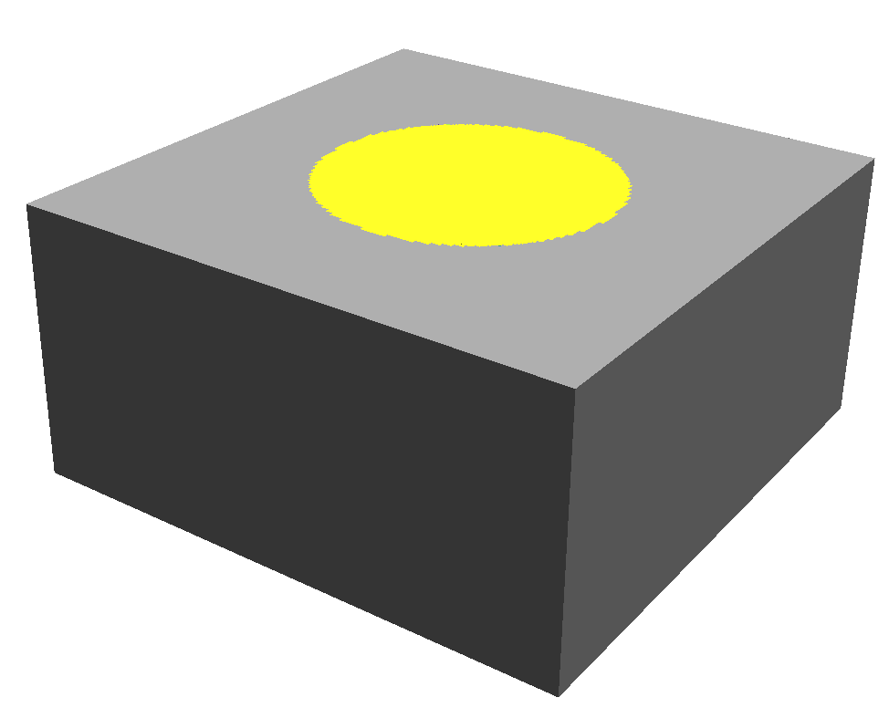
Figure 3: Representative initial configuration for the numerical results presented within this section. The yellow circle shows the location beneath the wave guide, i.e. the region of incident MMWs.

In order to validate the model described in section II, a comparison to experimental data is considered. Although MMW is still an emerging technology and experimental data is scarce, the study of Oglesby Oglesby et al. (2014) provides detailed temperature measurements for the heating of granite through a varying MMW source. This experiment considers a source upon a flat surface of granite, where the edges of the rock are sufficiently far from the incident beam that they are not heated. A sample geometry used in the numerical simulations is shown in figure 3, where a cuboidal geometry is used for simplicity given the underlying Cartesian coordinate system, and the region subject to incident MMWs is shown in yellow.

Figure 4: Comparison of the power recorded at the surface in the experiment of Oglesby Oglesby et al. (2014) (black line) and the values used in this work (red line). Several distinct changes in power are clear; the input power for this work uses an average through each of these regions.

The variations in the MMW source were measured at the surface over the course of the experiment (a duration of 30 minutes), with several clear, sharp changes in the power of the gyrotron. This profile is shown in figure 4, and is compared to the approximation to this profile used in this work. Due to the noisy nature of the measurements, average values are taken over each distinct region within the profile. These values are quantified in table 2. The remaining parameters for the power input and the domain used for this study are given in table 3.

Time (s)	Power (W)
0 - 150	800
150 - 390	1800
390 - 510	2300
510 - 750	2800
750 - 850	1700
850 - 1050	2800
1050 - 1200	1700
1200 - 1250	3200
1250 - 1750	0

Table 2: Time-varying power profile used in simulations reproducing the experiment of Oglesby Oglesby et al. (2014).

Simulation parameters
Domain size (m3)	$0.1\times 0.1\times 0.025$
$T_{0}$ (K)	297.5
$\omega_{0}$ (m)	$0.20$

Table 3: Simulation parameters used to reproduce the experiment of Oglesby Oglesby et al. (2014).

For this validation study, because the power was recorded at the surface itself, the stand-off distance described in section II is set to zero. In addition to measuring the power incident on the surface, the temperature here was also recorded at the centre of the incident source. This was done by measuring the thermal emission, $\varepsilon T$, using a 137 GHz radiometer. An illustration of the computational domain, and the location at which temperature is computed in simulation results, comparable to experiment, is given in figure 5.

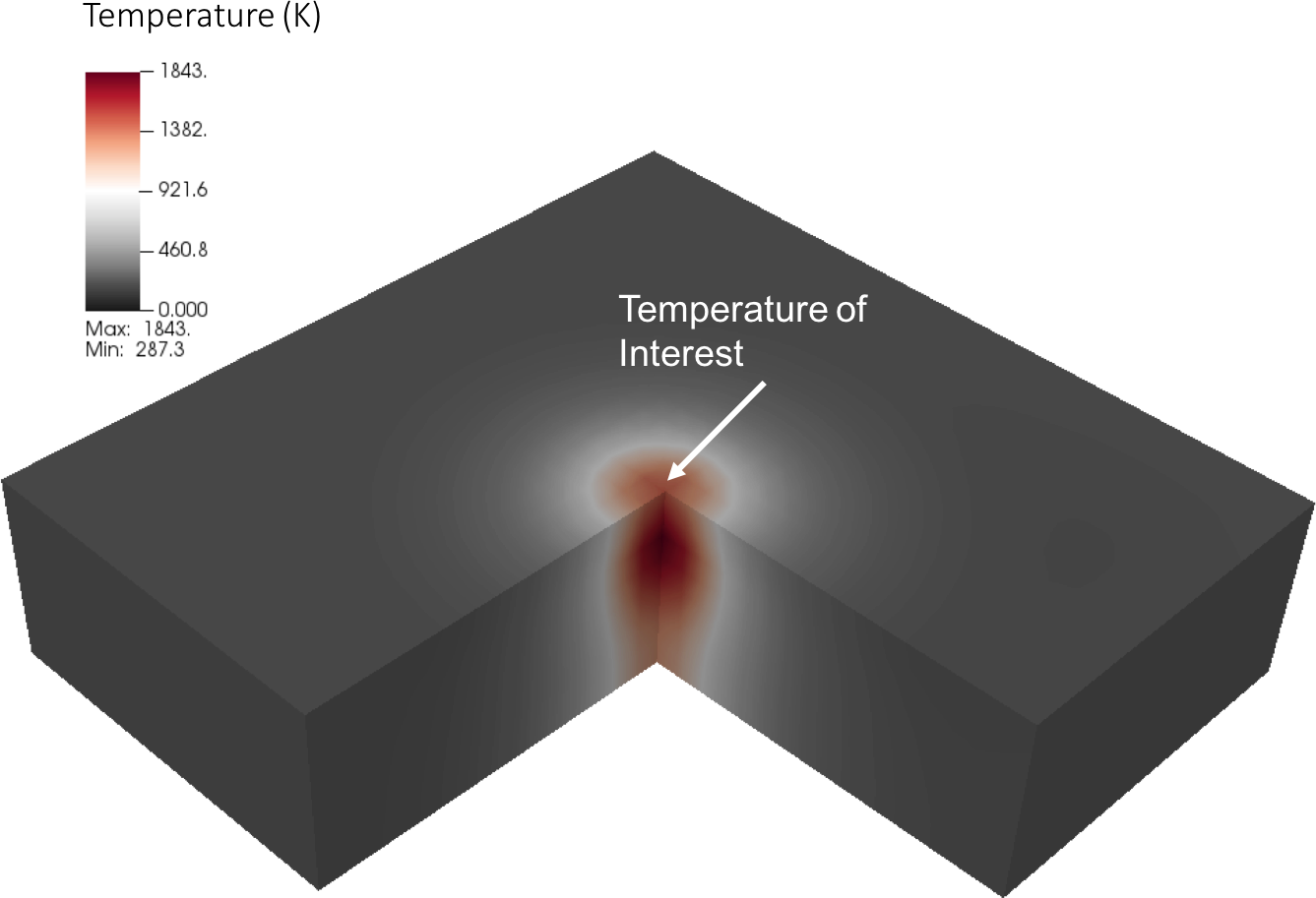
Figure 5: Illustration of the computational domain for comparison to the experiment of Oglesby Oglesby et al. (2014). The domain is cuboidal and a section has been removed to illustrate the full temperature profile through the rock. The arrow illustrates the centre of MMW beam where the surface temperature is recorded.

Material parameters are given by the relationships in section II. Melt Larsen (1929) and vaporisation Bronshten (2012) temperatures ($T_{m}$ and $T_{v}$ respectively) are given by

$$T_{m}=1488-1533\text{\ K},\quad T_{v}=3233-3503\text{\ K}.$$ (16)

where the range in values results in differences in composition of the rock; in this work the mid-point of these values is used.

Density of granite is given by equation (8) where

$$a_{\rho}=-0.2877\text{\ kg/(m${}^{3}$K)},\quad b_{\rho}=2884\text{\ kg/m${}^{3}$}$$ (17)

and above $T=1273$ K, a constant value of $\rho=2300$ kg/m³ is used. Thermal conductivity is given by equation (9) where

$$a_{\kappa}=0.3154\text{\ m K/W},\quad b_{\rho}=3.8\times 10^{-4}\text{\ m/W}$$ (18)

and above $T=1073$ K, a constant extrapolation is used. Specific heat is given by equation (11) with

$$a_{c}=-2.73\times 10^{4}\text{\ J K/kg},\quad b_{c}=0.894\text{\ J/kg}$$

$$c_{c}=788\text{\ J/(kg K)},\quad d_{c}=0.184\text{\ J/kg},\quad e_{c}=1249\text{\ J/(kg K)},$$ (19)

with a cut-off temperature of $T_{c}=T_{m}$. Latent heat of fusion of granite is $\xi_{f}=3.4\times 10^{5}$ J/kg and since solidus and liquidus temperatures are not available for granite, in order to ensure these contributions occur over a sufficient temperature range for algorithmic stability, latent heat is spread over 200 K around melt temperature. Latent heat of vaporisation is $\xi_{v}=4.8\times 10^{6}$ J/kg, and, as detailed in section II, it is spread over a range of 270 K from evaporation temperature onwards. The absorptivity of solid granite used in this work is $\alpha_{\lambda}=14$ Np/m, and for liquid granite, $\alpha_{\lambda}=56$ Np/m. Finally, the radiative emissivity of granite is given by $\varepsilon=0.7$ for $T\leq T_{m}$ and $\varepsilon=0.3$ for $T>T_{m}$, and a convective heat transfer coefficient of $h=56$ W/(m² K) is used, as given by Woskov and Michael Woskov and Michael (2012) and Oglesby Oglesby et al. (2014).

Figure 6: Comparison between experimental and simulation results for the temperature at the surface of the rock, directly beneath the MMW source. It is noted that a correction to the experimental temperatures has been made to account for material emissivity Oglesby et al. (2014). There is a good agreement between the two sets of results, the numerical model reproduced both the magnitude of the temperature, and the rise or fall behaviour as the incident power changes.

The comparison between experimental and simulation results is shown in figure 6. In order to make a direct comparison between the two results, an emissivity correction is required; the experimental measurements are recorded from the thermal radiation above the surface, and hence the true temperature of the surface is higher. The true value of any such correction is not yet known, and would require further experimental measurements, however, a value of 0.7 is used in figure 6 and this demonstrates a good agreement between simulation and experiment. The results also demonstrate that the behaviour when the input power is either increased or decreased matches the experiment. When the power changes, there is a sharp rise in temperature at the surface which then tails off. However, over this tailing off region, the temperature continues to either rise, or fall, gradually (following either an increase or a decrease respectively). This behaviour is captured in the simulation, suggesting the heating behaviour of the material is correctly modelled.

V Evaluation of the model

V.1 Single material configurations

Having validated the numerical model, it is now used to evaluate the material removal process for an isotropic, single material substrate. In these test results, in order to ensure computational efficiency, a very high source power is used. Though unphysical for any current gyrotron, the qualitative thermal behaviour will effectively be unchanged from more realistic configurations, but will happen over shorter time scales. The simulation parameters are given in table 4, with material properties as described in section IV.

Simulation parameters
Domain size (m3)	$1\times 1\times 2$
Simulation time (s)	$3.3$
$T_{0}$ (K)	297.5
Material	Granite
$P_{0}$ (W)	$1.7\times 10^{10}$
$\omega_{0}$ (m)	$0.22$

Table 4: Initial data for evaporation of granite under a high-powered MMW source.

Figure 7: Temperature profile for granite under an MMW source with conditions as given in table 4 over the course of the simulation. A slice is removed from the domain to show internal behaviour. The high powered source removes material rapidly, and diffusion throughout the rock is minimal over these time scales.

The temperature evolution within the granite for the test with initial data described by table 4 is shown in figure 7 at three snapshots in time. In this isotropic, single-material case, the geometry of the wellbore closely correlates with the Gaussian shape of the MMW source, which has been captured smoothly over the course of the simulation. Due to the very high power of the MMW source in this example, the material heating and removal happens over a faster time scale than temperature diffusion, hence there is a strong temperature gradient at the edges of the wellbore, which is captured in a non-oscillatory manner by the underlying numerical techniques.

V.2 Effect of absorption coefficient on wellbore structure

The results shown in figure 7 are for an isotropic granite material, and show the absorptive properties of the rock, as described in section IV. However, there are many ways where absorptivity is altered, typically due to changes in the emissivity or the electrical conductivity of the rock, which govern the overall absorptivity, shown in equation (12). Additionally, magnetic permeability may also have an effect, though this is only a consideration in magnetised materials, which are less commonly encountered. When considering MMW drilling within granite, it is common to encounter regions with high quartz content, which can be of concern due to the low absorptivity of quartz. Electrical conductivity can be increased for a wider range of materials if the rock is fractured and in particular if there is water saturation, which would typically result in a rise in the absorption coefficient.

For geothermal drilling processes, the regions of low absorptivity are of greatest concern; these could take longer to drill through, and there may then be non-uniform heating with respect to the neighbouring material, and thus a similarly non-uniform wellbore shape. To investigate the effects of this behaviour, a test simulation is considered with a very low absorption coefficient, $\alpha_{\lambda}=0.7$ Np/m, and compared to the results shown in figure 7.

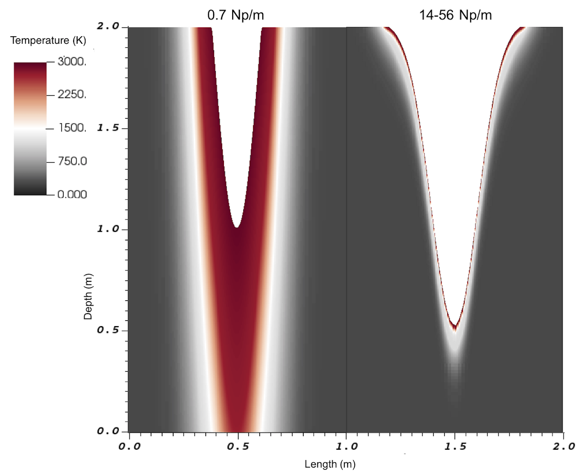
Figure 8: Comparison between the thermal profile of materials with different absorptivity, showing a slice through the centre of the computational domain. Both results are shown after 3.3 s with the left plot showing a material with $\alpha_{\lambda}=0.7$ Np/m, whilst the right plot shows granite values for $\alpha_{\lambda}$ given in section IV. The low absorptivity results in heating over a greater volume, and this subsequently results in a lower volume of material removed at a given time.

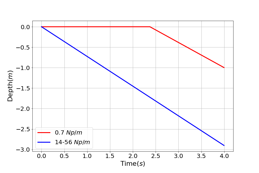
Figure 9: Penetration depth as a function of time for two different absorptivities. Whilst the lower absorptivity material takes longer to start melting, the actual rate of penetration is then also slightly slower.

Figure 8 shows the thermal profile for an absorptivity of $\alpha_{\lambda}=0.7$ Np/m compared to an equivalent time for granite with the absorption properties given in section IV. The high absorptivity shows a strong thermal gradient at the surface, since power does not penetrate very far into the material. The lower absorptivity material has a much longer penetration depth of the MMW source, and therefore a greater volume of material is heated. The temperature rise per unit volume is then lower, and as a result, less material has been removed at a given time. Figure 9 compares the rate of penetration as a function of time. Quantitatively, rate of penetration, $\dot{d}$, is related to power density, $\varrho_{p}$ and the specific energy of vaporisation, $e_{v}$, through

$$\centering\dot{d}=\frac{\varrho_{p}}{e_{v}}\quad\quad e_{v}=c_{p,m}\left(T_{v}-T_{m}\right)+\xi_{v}\@add@centering$$ (20)

where $c_{p,m}$ is the specific heat of melt Tang, Yang, and Zhou (2014). In addition to the melting and vaporisation properties, this relationship depends on absorptivity, entering though a reduction in power density in the low-absorptivity case. This is clearly apparent in figure 9; once material reaches evaporation temperature, the actual rate of removal is then slower for the material with low absorptivity; for this high-power source, the rate of penetration for granite is 0.73 m/s, whilst for the low absorptivity material it is 0.61 m/s. For single, isotropic materials, absorptivity is therefore not a significant concern beyond the reduction in rate of penetration. However, the behaviour for anisotropic situations, where absorptivity is not constant in space, may result in either insufficient or unwanted removal of material; this can be considered through multi-strata simulations.

VI Multi-strata modelling

Whilst it is important to understand the evaporation behaviour, and to predict the rate of penetration, through uniform rock, being able to capture the behaviour at the transition between material or configurations will be required to develop understanding of the MMW drilling process. The model described in section II is able to incorporate arbitrary numbers and geometric configurations of materials, with material properties required for solving equation (1) defined through the material scalar parameter. To assess this capability, three tests are considered, each with a planar material interface defined by the surface

$$-0.5x+0.2y-z+1=0.$$ (21)

The first test case considers a basalt-granite interface where basalt is the upper material (the first material upon which MMWs are incident), and all parameters for granite as given in section IV.

For basalt, melt Larsen (1929) and vaporisation Bronshten (2012) temperatures are given by

$$T_{m}=1257-1533\text{\ K},\quad T_{v}=3233-3503\text{\ K}.$$ (22)

where, as with granite, the range is dependent on the actual composition of the basalt, hence again the mid-point value is used. The density follows equation (8) with constants given by

$$a_{\rho}=-0.06\text{\ kg/(m${}^{3}$K)},\quad b_{\rho}=2897\text{\ kg/m${}^{3}$}$$ (23)

and above $T=933$ K, a constant value of $\rho=2801$ kg/m³ is used. Thermal conductivity is given by equation (10) where

$$c_{\kappa}=1.719\times 10^{-6}\text{\ W K/m},\quad d_{\rho}=-3.588\times 10^{-4}\text{\ W/m}$$

$$e_{\rho}=3.071\text{\ W/(m K)}$$ (24)

and above $T=T_{m}$, a constant extrapolation is used. Specific heat follows equation (11) with

$$a_{c}=-7.52\times 10^{4}\text{\ J K/kg},\quad b_{c}=1.43\text{\ J/kg}$$

$$c_{c}=415\text{\ J/(kg K)},\quad d_{c}=0.176\text{\ J/kg},\quad e_{c}=924\text{\ J/(kg K)},$$ (25)

with a cut-off temperature of $T_{c}=T_{m}$. Latent heat of fusion of basalt is $\xi_{f}=4.2\times 10^{5}$ J/kg and, as with granite, this is spread over 200 K around melt temperature, and latent heat of vaporisation is $\xi_{v}=4.0\times 10^{6}$. The absorptivity of solid basalt is $\alpha_{\lambda}=14$ Np/m, and for liquid basalt, $\alpha_{\lambda}=28$ Np/m. The parameters for radiative and convective losses in basalt have not been measured extensively, hence in this work, we assume that $\varepsilon=0.5$ and that the convective heat loss coefficient of granite, $h=56$ W/(m² K), can be used for basalt.

This configuration is motivated by the fact that basalt formed from volcanic eruptions overlays granite which originated from magma intrusion. The second test uses an absorptivity of $\alpha_{\lambda}=0.7$ Np/m for basalt, investigating the effects of a low-absorptivity region on top of a high-absorptivity one. The third test reverses this configuration, using $\alpha_{\lambda}=0.7$ Np/m for granite instead. The remaining initial data for these configurations is given in table 5.

Simulation parameters
Domain size (m3)	$1\times 1\times 1$
Simulation time (s)	$3$
$T_{0}$ (K)	297.5
$P_{0}$ (W)	$10^{9}$
$\omega_{0}$ (m)	$0.22$

Table 5: Initial data for evaporation of a multi-strata configuration.

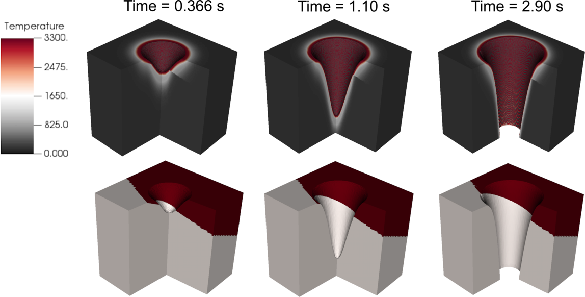
Figure 10: Simulation results for a basalt layer on top of granite. A section of the domain is removed to show internal behaviour of temperature (top), and the material, were red shows basalt and beige shows granite (bottom). The wellbore follows a Gaussian profile with minimal change at rock interface. However, the effects of the change in material are visible in temperature, with a discontinuity along basalt-granite interface, which correlates with an increase in MMW absorptivity moving from molten basalt to granite.

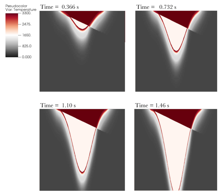
Figure 11: Cross section through the centre of the wellbore for the case of a basalt layer on granite, shown in figure 10. The temperature profile is shown for the solid and liquid phases, whilst the material (and hence interface) is plotted within the wellbore itself. The change in temperature gradient between the two materials is clear, though the shape of the wellbore remains largely symmetric.

Figure 10 shows the simulation for basalt on granite. The two materials have comparable properties, and this shows in the relatively smooth nature of the wellbore. However, the lower absorptivity of molten basalt is apparent in the slightly wider high-temperature region, i.e. there is a shallower temperature gradient. This behaviour is visible more clearly in figure 11, showing a cross section through the centre of the domain. These results, along with the implications for the rate of penetration from figure 9, suggest that these interfaces between similar igneous rock types will not be a major issue for MMW drilling applications.

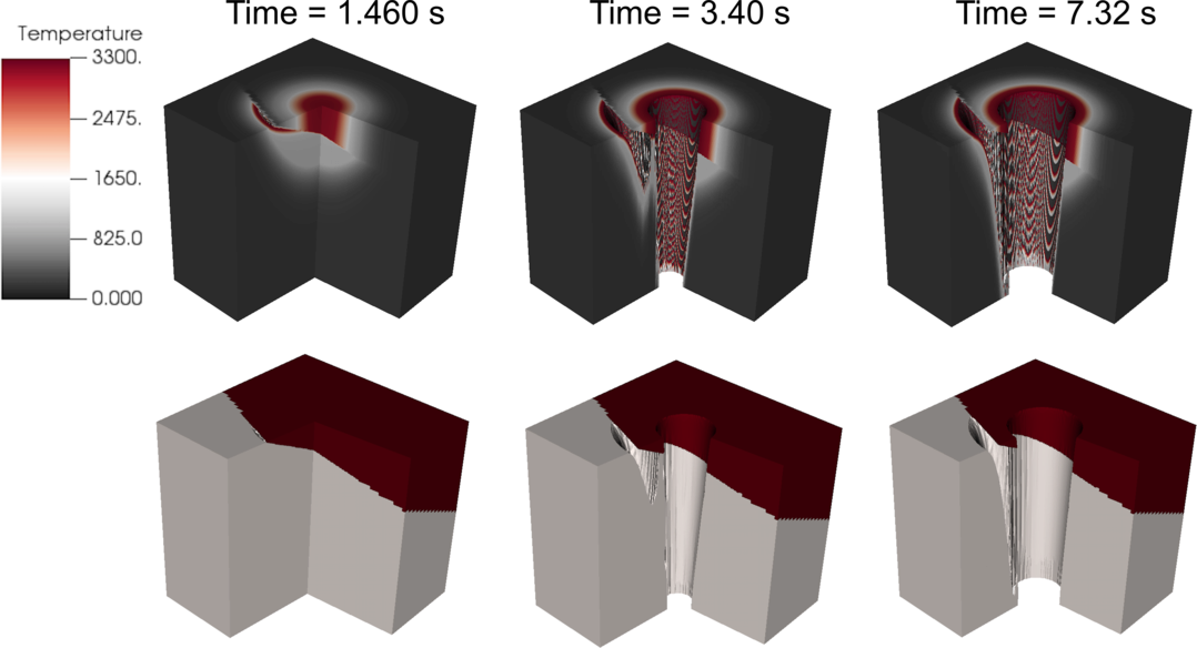
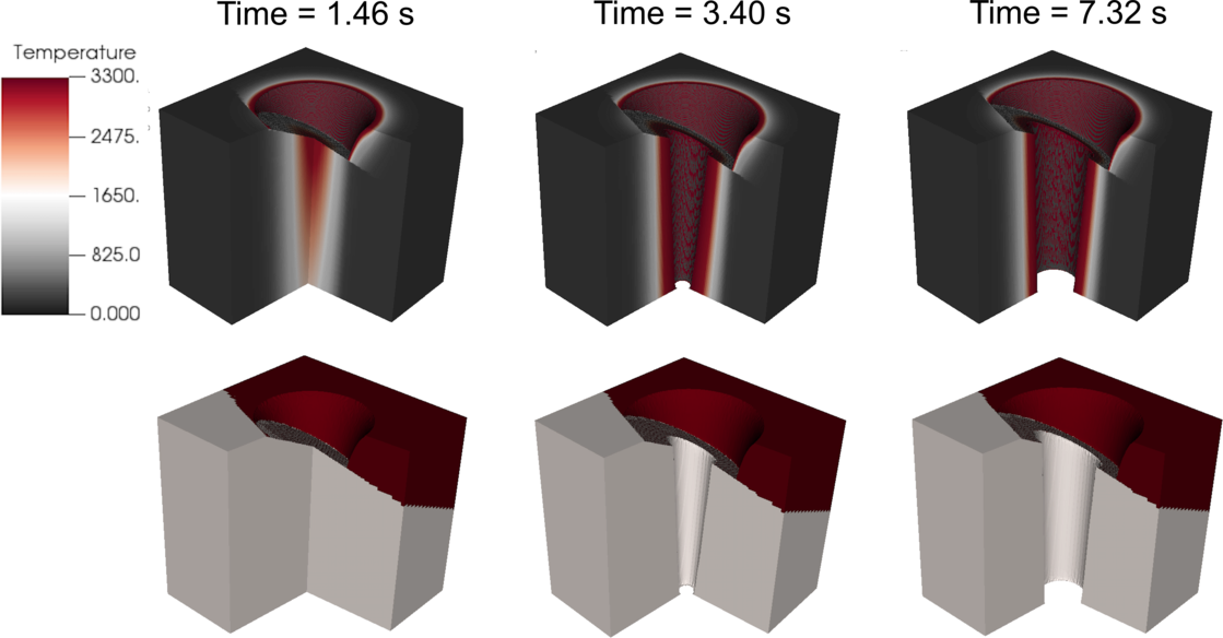
Figure 12: Simulation results for the multi-strata test cases with a low-absorptivity region; the top figure shows this region on top of granite, whilst the bottom figure shows basalt on top of a low absorptivity layer. In the top figure, it is clear that the radial growth of the wellbore is inhibited by the low-absorptivity layer. In the bottom case, the lower rate of expansion leads to the continued widening of the borehole through the basalt region on top.

In figure 12, the effects of replacing one of the strata with a low absorptivity material are demonstrated. In the top image in this figure, a case of a low absorptivity region above granite is shown. In this case, there is an overall reduction in the wellbore diameter and this corresponds to a slower evaporation of the granite beneath this layer. In general, the energy absorption by the low absorptivity layer is sufficient to prevent any direct melt of the granite beneath it. However, where this layer is sufficiently thin, then melting initially occurs beneath the surface. The model presented within this work can predict the onset of such behaviour, though at this point, additional techniques may be required to correctly simulate the resultant behaviour. In particular, a pressure build-up would be expected within this region, which is not accounted for in this thermal approach.

The third test case, in which the lower material has low absorptivity, is shown in the bottom image in figure 12. In this case, at early times, the expected behaviour is observed, in which the basalt region is removed much more rapidly, and then a new, angled surface heats up. At later times, the heat flux from the MMW source mostly interacts with the low absorptivity surface, though there is continued widening of the wellbore in the basalt region. In this configuration, the radius of the wellbore in this basalt region would then be larger than expected, which may have implications on equipment placed down the borehole.

These two test cases, though considering idealised materials, demonstrate that the model presented here can deal with sudden changes in material behaviour. In particular, it is possible to predict the effects of a change in one material on both the local rate of penetration behaviour, but also in the effects on neighbouring materials. In all cases, the numerical model has demonstrated that it can robustly deal with material changes within the domain. These changes are handled in a smooth manner, without generating oscillations. This gives confidence that this model can now be applied for geologically realistic configurations.

VII Conclusions

In this work, a thermal model for material evaporation through an MMW source has been presented, with a view to an application for drilling through geological materials. Of particular interest is igneous rock, for which conventional drilling methods struggle, and this has formed the basis of the validation, and subsequent evaluation of the model.

Validation was based on the experiment of Oglesby Oglesby et al. (2014), for which a slab of granite was subjected to heating through a kilowatt MMW gyrotron source. This heating lasted 30 minutes, and the incident power was changes several times over the course of the experiment. It was demonstrated in section IV that the model presented here could match the thermal profile recorded from this experiment; both temperature values and the equilibration of these values as surface heat losses matched the incident power were shown.

The model was then utilised in section V.1 to investigate effects of evaporation of materials with differing absorptive properties. It was identified that a lower absorption coefficient delayed the onset of evaporation, and subsequently resulted in a slower rate of penetration. One of the key advantages of this model is that it allows for an arbitrary geometric configuration of different rock types, or regions with different physical properties. This was investigated in section VI, where a typical basalt-on-granite configuration was studied, as well as a more extreme case, with a strata of low-absorptivity rock. This latter case is of interest for cases such as granite with high quartz content; quartz allowing for more transmission of MMW radiation. In this case, the multi-strata simulations were handled smoothly, and able to demonstrate the differences in wellbore structure in all cases.

The work presented here highlights several areas for further study, as well as additional developments to further increase the applicability of the model. Two types of rock, basalt and granite, were considered here, and success at the model for dealing with these materials means work can in future be extended to more rock types. However, this extension, as well as improving accuracy of the current results, requires further experimental study into the material properties of rocks at high temperatures. As discussed in section II, the properties of these materials are generally only well-studied up to around 1000 K, whilst the MMW drilling approach is expected to evaporate the rock, with temperatures exceeding 3000 K. Simple constant or linear extrapolations of the known data were used in this work, and were demonstrated to produce a good physical description of the material. However, extending the knowledge of the thermal properties of rocks to higher temperature ranges, and to more rock types, would have an obvious benefit to the results presented in this work.

In section III.2, the importance of the surface treatment was considered. Within the thermal approach, the heating and evolution of gas needs to be imposed as a surface condition, a variety of options were considered, guided by the experimental results of Oglesby Oglesby et al. (2014). These conditions could, in future, be augmented by coupling the model to a gas flow simulation, which would allow the effect on surface cooling of imposed gas flow scenarios to be simulated. This could then identify optimal conditions for rate of penetration whilst preventing plasma formation in the gas beneath the wave guide.

The work presented here has assumed that the absorption coefficient, $\alpha_{\lambda}$ is constant, or at least piece-wise constant. This is an assumption that simplifies the power input; allowing it to be expressed as a function of height only. In practice, the absorption coefficient depends on temperature, and as a result there is a non-uniform absorption of power with depth. This requires an integral approach, where power absorbed is not dependent only on the power incident on the surface, but of that absorbed by material above the height of computation. This can be challenging, given that the height of the surface is not constant; the power absorbed needs to be integrated with respect to depth for every point in the $(x,y)$-plane. Within this framework, such a technique could be incorporated into future work, taking advantage of the fast-sweeping algorithm for the signed distance function; this algorithm itself performs an extrapolation from the surface outwards, and hence the computational framework exists to achieve this extension. This has the additional advantage that power absorption can be computed even for complex AMR grid structures, where information transfer concerns exist.

This proposed future development would also allow inhomogeneities within the rock strata to be considered. Here, local changes in properties, including absorption, could be incorporated, either as distinct crystalline structures, or a macroscopic averaging, depending on the length-scales required. The generation of suitable anisotropic structures has been considered at crystal grain-scales by Toifl et al. Toifl et al. (2016) and Quey et al. Quey, Dawson, and Barbe (2011), whilst larger scale approximations have been considered by Tang et al. Tang, Yang, and Zhou (2014) In addition to the development proposed for absorptive properties, the scalar parameter for modelling material type used in this work would allow these techniques to be incorporated into the model presented here.

These considerations for future work would enhance the capabilities of this work to simulate the evaporation complex geological materials under a MMW source. The work described within this paper describes a novel technique which underlies these ideas, and itself augments the experimental studies of MMW drilling using gyrotrons, allowing for a rapid investigation of parameter space, both for the source and the substrate. The adaptive meshing approach, which does not depend on assumptions as to the wellbore shape or growth rate, allows for computationally efficient, large-scale simulations.