Flavor-changing light bosons with accidental longevity

Abstract

We consider a model with a complex scalar field that couples to $(e,\mu)$ or $(\mu,\tau)$ within the “longevity” window: $[|m_{l_{1}}-m_{l_{2}}|,m_{l_{1}}+m_{l_{2}}]$ in which $l_{1}$ and $l_{2}$ are the two different charged leptons. Within such a mass window, even a relatively large coupling (e.g. of the size commensurate with the current accuracy/discrepancy in the muon $g-2$ experiment) leads to long lifetimes and macroscopic propagation distance between production and decay points. We propose to exploit several existing neutrino experiments and one future experiment to probe the parameter space of this model. For the $\mu-e$ sector, we exploit the muonium decay branching ratio and the production and decay sequence at the LSND experiment, excluding the parametric region suggested by $g_{\mu}-2$ anomaly. For the $\tau-\mu$ sector, we analyze three main production mechanisms of scalars at beam dump experiments: the Drell-Yan process, the heavy meson decay, and the muon scattering. We explore the constraints from the past CHARM and NuTeV experiments, and evaluate sensitivity for the proposed beam dump experiment, SHiP. The latter can thoroughly probe the parameter space relevant for the $g_{\mu}-2$ anomaly.

1 Introduction

Lepton flavor is an accidental symmetry which is exactly conserved in the SM with massless neutrinos. The observation of neutrino oscillation and the non-vanishing neutrino mass have firmly established the existence of neutral lepton flavor transitions. This provides strong motivation to search for the charged lepton flavor violation (CLFV). In the Standard Model (SM), the CLFV is suppressed by $G_{F}^{2}m_{\nu}^{4}\leq 10^{-50}$ which is tiny and beyond the sensitivity of any experiments. Thus, any observation of CLFV must imply new physics beyond Standard Model. There has been a great interest in searching CLFV in various experiments (see recent review like Davidson:2022jai ). In the next decades, the experimental search can be greatly improved by the new generation of experiments such as MEG II, Mu3e, COMET and Mu2e Meucci:2022qbh ; Chiappini:2021ytk ; Mu2e:2014fns ; Hesketh:2022wgw ; COMET:2018auw . It is also expected that Belle-II Belle-II:2018jsg experiment will collect around $5\times 10^{10}$ events with $\tau^{\pm}$ pairs, which is one order enhancement compared to Belle Belle:2012iwr and BaBar BaBar:2001yhh . Additional support for the search of the charged lepton flavor violation comes from the ongoing discrepancy between the measured and predicted anomalous magnetic moment of the muon, which may indicate presence of New Physics in the muon sector.

Theoretically, there are various ways to realize the CLFV in the new physics sector at different energy scales. Flavor off-diagonal contribution can originate from heavy degrees of freedom. For example, the flavor non-diagonal SUSY breaking terms, and R-violation terms Paradisi:2005fk ; Girrbach:2009uy ; Hisano:2001qz ; Babu:2002et can generate Lepton Flavor Violation (LFV) terms. For the purpose of low-energy physics, one can integrate these heavy degrees of freedom out and parametrize the LFV in terms of the higher dimensional operators. The complete sets of dimension-six operators can be found in e.g. Crivellin:2013hpa . This way, precision constraints on branching ratios of multiple rare decay processes can be translated to limits on the corresponding Wilson coefficients in the effective theory. An interesting alternative to this approach exists in theories with light beyond SM states that can mediate such flavor transitions. This results in a somewhat richer phenomenology, with the possibility of studying the production and decay of such light states using various experimental techniques.

There are many well-known theoretical models which can provide such kinds of couplings. One well-known example is the axion or axion-like particles (ALP). It was originally postulated to solve the QCD strong CP problem and can be defined as the pseudo-Nambu-goldstone boson from the spontaneous breaking of the Peccei-Quinn symmetry at some high scale $f_{a}$. Subsequently, the QCD axion has been generalized to an ALP, and its mass could cover a wide range of scales from ultralight sub-eV scales to above the electroweak scale. An ALP can couple to leptons and quarks off-diagonally, thus leading to flavored $l_{1}-l_{2}-a$ couplings Wilczek:1982rv ; Ema:2016ops ; Calibbi:2016hwq ; Bonnefoy:2020llz ; Bauer:2021mvw ; MartinCamalich:2020dfe ; Calibbi:2020jvd . An exchange of real ALP will then generate $l_{1}l_{1}\to l_{2}l_{2}$ LFV transitions. Similarly, the pseudo-scalar Majoron and familon Farzan:2002wx ; Kachelriess:2000qc ; Lessa:2007up ; Wilczek:1982rv ; Reiss:1982sq ; Chang:1987hz , which are the Goldstone boson relevant to the breaking of the global lepton number and global family symmetry, can also make contributions to LFV.

In this paper, we will introduce a flavor changing scalar (FCS) with the flavor off-diagonal coupling as a possible solution to the on-going discrepancy between SM prediction and measurement of $(g-2)_{\mu}$ Muong-2:2002wip ; Muong-2:2004fok ; Muong-2:2006rrc ; Davier:2017zfy ; Colangelo:2018mtw ; Hoferichter:2019mqg ; Davier:2019can ; Keshavarzi:2019abf ; Aoyama:2020ynm ; Muong-2:2021ojo . It is well known that one loop correction to $(g-2)_{\mu}$ resulting from a ALP loop is typically of a “wrong” sign of curing the anomaly if ALP has a flavor-diagonal coupling. If, on the other hand, the coupling connects two different flavors, the sign of the correction can be positive, and one could consider such a model as a candidate solution to the muon $(g-2)_{\mu}$ discrepancy. (One has to remark at this point that the status of the discrepancy was questioned recently by the lattice QCD results, which came much closer to the observed value Borsanyi:2020mff .)

Let us consider the $l_{1}-l_{2}-\phi$ coupling between an FCS and two leptons ($m_{l_{1}}<m_{l_{2}}$) in the range relevant for the $(g-2)_{\mu}$ correction. Then, with respect to a possible mass ordering of $\phi$, one can point to the three main regimes:

$$m_{\phi}<m_{l_{2}}-m_{l_{1}},~{}~{}~{}{\rm prompt~{}decay~{}of}~{}l_{2},$$ (1)

$$m_{l_{2}}-m_{l_{1}}<m_{\phi}<m_{l_{2}}+m_{l_{1}}~{}~{}~{}{\rm longevity~{}window},$$ (2)

$$\ m_{\phi}>m_{l_{2}}+m_{l_{1}}~{}~{}~{}{\rm prompt~{}decay~{}of}~{}\phi.$$ (3)

The first regime leads to fast decays of $l_{2}\to l_{1}+\phi$, and is generally excluded for the range of coupling of interest by the lifetime of $l_{2}$, while the third regime leads to the prompt decay of $\phi$. The longevity window is when neither of the two-body decays, $l_{2}\to l_{1}+\phi$ and $\phi\to l_{2}+l_{1}$ are allowed. In this window, $\phi$ is long-lived despite sizable coupling provided that $l_{1}-l_{1}-\phi$ coupling is forbidden.

This paper mainly considers a simple FCS model with flavor off-diagonal transitions in the lepton sector. A light complex scalar $\phi$ is introduced, which directly couples to $(\mu e)$ or $(\tau\mu)$. Instead of breaking the lepton flavor symmetry at the Lagrangian level, we assign the complex scalar to carry both the charged lepton charge with opposite signs. For the sake of generality, we do not assume the new boson is scalar or pseudoscalar, but the scalar and axial coupling are both turned on.

We show that lepton $g-2$ experiments provide sensitive probe of $l_{1}-l_{2}-\phi$ vertex. In addition, $\phi$ particle longevity opens an interesting possibility for the beam dump studies of $\phi$. While the off-diagonal $e\mu$ coupling can be efficiently studied at intense sources of muons, the $\mu\tau$ case can be probed directly at the proton beam dump facilities and neutrino experiments. We analyze three different mechanisms of $\phi$ production: electroweak production in the target, production through fragmentation of charged mesons, and secondary muon-initiated production. We then exploit the results of the existing experiments (LSND LSND:1996jxj ; LSND:2001akn , NuTeV NuTeV:2001ndo ; NuTeV:2001ndo ; NuTeV:2005wsg and CHARM CHARM:1985nku ), to set competitive constraints on the parameter space of the model. It turns out that using existing experimental results, one can derive direct constraints on $e-\mu-\phi$ coupling that are better than indirect ones obtained via muon $g-2$. At the same time, indirect constraints on $\mu-\tau-\phi$ coupling are stronger than the direct ones. We also derive projections for the SHiP experiment Alekhin:2015byh ; SHiP:2020hyy , and show that it can be used to probe the muon $g-2$ relevant window of couplings.

The rest of this paper is organized as follows. In Sec 2, we introduce the more detailed model description and establish the connection to the magnetic moment observables. Then we analyze the signatures of the model for a variety of past, current and proposed experiments. We cover the $\mu-e$ case in Sec. 3, and $\tau-\mu$ case in Sec. 4. We reach our conclusions in Sec. 5.

2 Preliminaries

In this section, we summarize the basic ingredients of our setup. We describe the model with a complex scalar field $\phi$ in Sec. 2.1. We then compute various electromagnetic moments that $\phi$ induces, with an emphasis on the muon anomalous magnetic moment in Sec. 2.2.

2.1 Model description

The ongoing discrepancy between the SM prediction and the measured value of the muon $g-2$ motivates an extension of the SM in the muon sector. In this paper, we consider a complex scalar field $\phi$ that couples to leptons

$$\mathcal{L} =\left\lvert\partial\phi\right\rvert^{2}-m_{\phi}^{2}\left\lvert\phi\right\rvert^{2}+\phi\,\bar{\mu}\left(g_{V}+g_{A}\gamma_{5}\right)l+\phi^{*}\bar{l}\left(g_{V}^{*}-g_{A}^{*}\gamma_{5}\right)\mu,$$ (4)

where $l$ is either $e$ or $\tau$. We assume that $\phi$ has $L_{\mu}$ charge $+1$ and $L_{l}$ charge $-1$ so that only the couplings with different generations of leptons are allowed. This Lagrangian may originate from

$$\mathcal{L} =\left\lvert\partial\phi\right\rvert^{2}-m_{\phi}^{2}\left\lvert\phi\right\rvert^{2}+\frac{\partial_{\mu}\phi}{\Lambda}\bar{\mu}\gamma^{\mu}\left(\tilde{g}_{V}-\tilde{g}_{A}\gamma_{5}\right)l+\frac{\partial_{\mu}\phi^{*}}{\Lambda}\bar{l}\gamma^{\mu}\left(\tilde{g}_{V}^{*}-\tilde{g}_{A}^{*}\gamma_{5}\right)\mu,$$ (5)

that has only derivative interactions between $\phi$ and SM leptons. Indeed, after using the equation of motion of the leptons we reproduce Eq. (4). As stated in the introduction, throughout this paper, we focus on the mass range

$$\left\lvert m_{\mu}-m_{l}\right\rvert<m_{\phi}<m_{\mu}+m_{l}.$$ (6)

Although relatively a limited mass range, this window provides interesting phenomenological signatures. The lower bound prohibits two-body decay $\mu\to\phi+e$ or $\tau\to\phi+\mu$, avoiding stringent constraints on the couplings, while the upper bound prohibits two-body decay $\phi\to\mu+l$, making $\phi$ accidentally long-lived. This model can explain the discrepancy of the muon anomalous magnetic dipole moment as we now see.

2.2 Muon anomalous magnetic moment

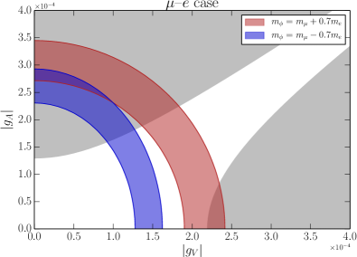
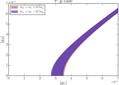
Figure 1: The parameter regions that explain the muon $g-2$ anomaly. Note that the magnetic dipole moments depend only on the absolute values of $g_{V}$ and $g_{A}$. Left panel: the $\mu\,\mathchar 45\relax\mathchar 45\relax\,e$ case. The red and blue regions explain the muon $g-2$ anomaly within $1\sigma$ with $m_{\phi}=m_{\mu}+0.7m_{e}$ and $m_{\phi}=m_{\mu}-0.7m_{e}$, respectively, as benchmarks. The gray region is excluded by the electron $g-2$ constraint (10). We have taken $m_{\phi}=m_{\mu}$ for the electron $g-2$ constraint in this figure, but the electron $g-2$ constraint has little dependence on $m_{\phi}$ within the mass range of our interest. Right panel: the $\tau\,\mathchar 45\relax\mathchar 45\relax\,\mu$ case. The red and blue regions explain the muon $g-2$ anomaly within $1\sigma$ with $m_{\phi}=m_{\tau}+0.7m_{\mu}$ and $m_{\phi}=m_{\tau}-0.7m_{\mu}$, respectively.

Recently the Fermilab muon $g-2$ experiment confirmed the Brookhaven result. The discrepancy between the experimental measurements and the SM prediction of the muon magnetic moment $a_{\mu}$ is now given by Davier:2017zfy ; Colangelo:2018mtw ; Hoferichter:2019mqg ; Davier:2019can ; Keshavarzi:2019abf ; Aoyama:2020ynm ; Muong-2:2021ojo

$$\Delta a_{\mu}=a_{\mu}^{\text{exp}}-a_{\mu}^{\text{SM}}=\left(251\pm 59\right)\times 10^{-11}.$$ (7)

In our model, $\phi$ contributes to the anomalous muon magnetic dipole moment at one-loop as

$$a_{\mu}^{(\phi)}=\frac{m_{\mu}}{8\pi^{2}}\int_{0}^{1}dz\frac{(1-z)^{2}\left[(\left\lvert g_{V}\right\rvert^{2}+\left\lvert g_{A}\right\rvert^{2})zm_{\mu}+(\left\lvert g_{V}\right\rvert^{2}-\left\lvert g_{A}\right\rvert^{2})m_{l}\right]}{-z(1-z)m_{\mu}^{2}+(1-z)m_{l}^{2}+zm_{\phi}^{2}}.$$ (8)

This contribution can explain the discrepancy (7) for both $l=e$ and $\tau$ cases, as shown in Fig 1. The above formula agrees with Endo:2020mev in the limit $m_{l}\ll m_{\mu},m_{\phi}$.

In our model, $\phi$ induces other electromagnetic dipole moments as well. In particular, $\phi$ induces the anomalous magnetic moment of $l$ as

$$a^{(\phi)}_{l} =\frac{m_{l}}{8\pi^{2}}\int_{0}^{1}dz\frac{(1-z)^{2}\left[\left(\left\lvert g_{V}\right\rvert^{2}+\left\lvert g_{A}\right\rvert^{2}\right)zm_{l}+\left(\left\lvert g_{V}\right\rvert^{2}-\left\lvert g_{A}\right\rvert^{2}\right)m_{\mu}\right]}{-z(1-z)m_{l}^{2}+(1-z)m_{\mu}^{2}+zm_{\phi}^{2}}.$$ (9)

The anomalous magnetic dipole moment of $\tau$ is only limited as $-0.052<a_{\tau}<0.013$ by LEP DELPHI:2003nah and thus we safely ignore the contribution of $\phi$ to $a_{\tau}$. In contrast, the anomalous magnetic dipole moment of $e$ is measured with extreme precision VanDyck:1987ay ; Odom:2006zz ; Hanneke:2008tm ; Fan:2022eto . Given the discrepancy between different measurements of the fine structure constant Parker:2018vye ; Morel:2020dww that is crucial for the SM prediction of $a_{e}$, we may require that the contribution from $\phi$ satisfies

$$-3.4\times 10^{-13}<a_{e}^{(\phi)}<9.8\times 10^{-13},$$ (10)

following Morel:2020dww . Since $a_{e}^{(\phi)}$ picks up the chirality flip from the internal muon unless the coupling is purely left-handed or right-handed, corresponding to the second term in the numerator of Eq. (9), the constraint on $a_{e}^{(\phi)}$ prefers $|{g_{V}}|\sim|g_{A}|$, as we show in Fig. 1. Therefore we focus on this parameter region in the $\mu\,\mathchar 45\relax\mathchar 45\relax\,e$ case. Moreover, $\phi$ induces the electric dipole moments (EDMs) of the muon and $l$ as

$$d_{\mu} =-\frac{\mathrm{Im}(g_{V}^{*}g_{A})m_{l}}{8\pi^{2}}\int_{0}^{1}dz\frac{(1-z)^{2}}{-z(1-z)m_{\mu}^{2}+(1-z)m_{l}^{2}+zm_{\phi}^{2}},$$ (11)

$$d_{l} =-\frac{\mathrm{Im}(g_{V}^{*}g_{A})m_{\mu}}{8\pi^{2}}\int_{0}^{1}dz\frac{(1-z)^{2}}{-z(1-z)m_{l}^{2}+(1-z)m_{\mu}^{2}+zm_{\phi}^{2}}.$$ (12)

The electron EDM is constrained with high precision ACME:2018yjb , while the muon and tau EDM can be constrained both directly and indirectly Belle:2002nla ; Muong-2:2008ebm ; Ema:2021jds ; Ema:2022wxd . For simplicity, we assume no CP violation, $\mathrm{Im}[g_{V}^{*}g_{A}]=0$, and ignore the EDMs in the following. Then we take both $g_{V}$ and $g_{A}$ real by redefining the phase of $\phi$ without loss of generality.

The result of this subsection sets the sizes of the couplings of interest. In the following, we will see that the whole parameter region is excluded by muonium invisible decay and the LSND experiment in the $\mu\,\mathchar 45\relax\mathchar 45\relax\,e$ case. Although previous and current experiments do not exclude the $\tau\,\mathchar 45\relax\mathchar 45\relax\,\mu$ case, the whole parameter space can be explored by future experiments such as SHiP.

3 $\mu\,\mathchar 45\relax\mathchar 45\relax\,e$ case: Muonium and LSND

In this section we consider the case that $\phi$ couples to $\mu$ and $e$, i.e. the $\mu\,\mathchar 45\relax\mathchar 45\relax\,e$ case. We will see that the muonium invisible decay branching ratio puts a constraint on the couplings. More interestingly, muonium formation and its subsequent decay produce a sizable flux of $\phi$ at neutrino experiments with muon decay at rest, such as the Liquid Scintillator Neutrino Detector (LSND) experiment. Even though $\phi$ has a huge decay length, as we see below, a small portion of $\phi$-decay inside the LSND detector is enough to exclude the entire parameter region that explains the muon $g-2$ anomaly.

3.1 Decay rates

In this subsection, we compute the decay rates of $\phi$ and muonium into $\phi$ that are necessary to understand the phenomenology of $\phi$.

3.1.1 $\phi$ decay rate

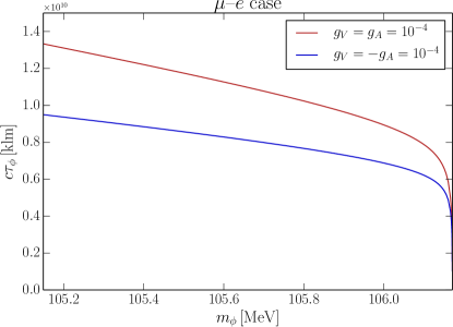
Figure 2: The decay length $c\tau_{\phi}$ of $\phi$ in the $\mu\,\mathchar 45\relax\mathchar 45\relax\,e$ case. The red line corresponds to $g_{V}=g_{A}=10^{-4}$ and the blue line to $g_{V}=-g_{A}=10^{-4}$. Note that the parameter region $\left\lvert g_{V}\right\rvert\simeq\left\lvert g_{A}\right\rvert$ is preferred from the electron $g-2$ constraint.

Since we consider the mass range $m_{\mu}-m_{e}<m_{\phi}<m_{\mu}+m_{e}$, the two-body decay $\phi\to\mu^{-}e^{+}$ is not allowed, and thus $\phi$ becomes accidentally long-lived. Instead, $\phi$ mainly decays as $\phi\to e^{-}e^{+}\nu_{\mu}\bar{\nu}_{e}$ through an off-shell $\mu^{-}$, whose amplitude is diagrammatically given by

$$i\mathcal{M}=\leavevmode\hbox to6.67pt{\vbox to6.67pt{\text{[drawing]}}}, {\scriptstyle\phi} {\scriptstyle e^{+}} {\scriptstyle e^{-}} {\scriptstyle\nu_{\mu}} {\scriptstyle\bar{\nu}_{e}} {\scriptstyle\phi} {\scriptstyle e^{+}} {\scriptstyle e^{-}} {\scriptstyle\nu_{\mu}} {\scriptstyle\bar{\nu}_{e}}$$ (13)

where the dot indicates the four-Fermi operator and the arrow indicates the flow of the muon number. The decay width of $\phi$ is given by (see App. A.1 for derivation)

$$\Gamma_{\phi} =\frac{G_{F}^{2}}{384\pi^{5}m_{\phi}}\int_{m_{e}^{2}}^{(m_{\phi}-m_{e})^{2}}\frac{d\bar{m}_{\mu}^{2}}{(\bar{m}_{\mu}^{2}-m_{\mu}^{2})^{2}}\int_{0}^{(\bar{m}_{\mu}-m_{e})^{2}}d\bar{m}_{\nu\nu}^{2}I_{1}(\bar{m}_{\mu},\bar{m}_{\nu\nu})$$

$$\times\left[\left(\left\lvert g_{V}+g_{A}\right\rvert^{2}\bar{m}_{\mu}^{2}+\left\lvert g_{V}-g_{A}\right\rvert^{2}m_{\mu}^{2}\right)I_{2}(\bar{m}_{\mu})-2(\left\lvert g_{V}\right\rvert^{2}-\left\lvert g_{A}\right\rvert^{2})m_{e}m_{\mu}\bar{m}_{\mu}^{2}I_{3}(\bar{m}_{\mu})\right],$$ (14)

where

$$I_{1} =\left(1+\frac{\bar{m}_{\nu\nu}^{2}-2m_{e}^{2}}{\bar{m}_{\mu}^{2}}+\frac{m_{e}^{4}+m_{e}^{2}\bar{m}_{\nu\nu}^{2}-2\bar{m}_{\nu\nu}^{4}}{\bar{m}_{\mu}^{4}}\right)\sqrt{\left(\bar{m}_{\mu}^{2}-\bar{m}_{\nu\nu}^{2}\right)^{2}-2m_{e}^{2}(\bar{m}_{\mu}^{2}+\bar{m}_{\nu\nu}^{2})+m_{e}^{4}},$$ (15)

$$I_{2} =\frac{m_{\phi}^{2}-\bar{m}_{\mu}^{2}-m_{e}^{2}}{4m_{\phi}^{2}}\sqrt{(m_{\phi}^{2}-\bar{m}_{\mu}^{2})^{2}-2m_{e}^{2}(m_{\phi}^{2}+\bar{m}_{\mu}^{2})+m_{e}^{4}},$$ (16)

$$I_{3} =\frac{\sqrt{(m_{\phi}^{2}-\bar{m}_{\mu}^{2})^{2}-2m_{e}^{2}(m_{\phi}^{2}+\bar{m}_{\mu}^{2})+m_{e}^{4}}}{2m_{\phi}^{2}}.$$ (17)

In this formula $G_{F}$ is the Fermi constant, $\bar{m}_{\mu}$ is the invariant mass of the off-shell muon, and $\bar{m}_{\nu\nu}$ is the invariant mass of the $\nu_{\mu}\bar{\nu}_{e}$ system, respectively. We plot the decay length of $\phi$ in Fig. 2. As one can see, $\phi$ has a huge decay length compared to the detector length due to the four-body decay phase space and the smallness of the couplings.

3.1.2 Muonium decay rate

Muonium is a hydrogen-like bound state consisting of $\mu^{+}$ and $e^{-}$. The mass range $m_{\mu}-m_{e}<m_{\phi}<m_{\mu}+m_{e}$ (ignoring the binding energy) allows muonium to decay into $\phi^{*}$ and photon. The muonium decay rate into $\phi^{*}\gamma$ can be written as

$$\Gamma(\mathrm{Mu}\to\phi^{*}\gamma) =\left\lvert\psi(0)\right\rvert^{2}\times\sigma_{\mathrm{free}}v(\mu^{+}e^{-}\to\phi^{*}\gamma),$$ (18)

where $\sigma_{\mathrm{free}}(\mu^{+}e^{-}\to\phi^{*}\gamma)$ is the annihilation cross-section of free $\mu^{+}$ and $e^{-}$ going to $\phi^{*}$ and $\gamma$, and $\psi(0)$ is the muonium wavefunction at the origin, given by

$$\left\lvert\psi(0)\right\rvert^{2} =\frac{\alpha^{3}m_{e}^{3}}{\pi},$$ (19)

for the ground state in the limit $m_{e}\ll m_{\mu}$. In the non-relativistic limit, we obtain (see App. A.2 for derivation)

$$\Gamma\left(\mathrm{Mu}^{(S=1)}\to\phi^{*}\gamma\right) =\frac{\alpha^{4}(\left\lvert g_{V}\right\rvert^{2}+\left\lvert g_{A}\right\rvert^{2})}{3\pi}\frac{m_{e}(m_{\mu}+m_{e}-m_{\phi})}{m_{\mu}},$$ (20)

$$\Gamma\left(\mathrm{Mu}^{(S=0)}\to\phi^{*}\gamma\right) =0,$$ (21)

where the superscripts $S=0$ and $1$ indicate the spin of the muonium. Here the selection rule works due to the angular momentum conservation, in a similar way as the positronium decay into photons. The muonium lifetime is dominated by the individual muon lifetime, and thus, the branching ratio is given by

$$\mathrm{Br}(\mathrm{Mu}^{(S=1)}\to\phi^{*}\gamma) =2.5\times 10^{-5}\times\frac{m_{\mu}+m_{e}-m_{\phi}}{m_{e}}\left(\frac{\left\lvert g_{V}\right\rvert^{2}+\left\lvert g_{A}\right\rvert^{2}}{10^{-8}}\right).$$ (22)

This rate is sizable since the decay into $\phi^{*}$ competes with the weak process, which results in $G_{F}^{2}$ in the denominator.

3.2 Constraints

We now discuss the constraints of our model. We will see that the parameter region that explains the muon $g-2$ anomaly is excluded by muonium invisible decay and by the LSND experiment.

3.2.1 Muonium invisible decay

As we saw above, muonium can decay into $\phi^{*}$ and $\gamma$, even though a free $\mu^{+}$ cannot decay into $\phi^{*}e^{+}\gamma$. Ref. Gninenko:2012nt sets a bound on such an invisible (i.e. $e^{+}$–less) decay branching ratio of muonium based on the results of the MuLan experiment MuLan:2007qkz ; MuLan:2010shf ; MuLan:2012sih . The MuLan experiment performed a dedicated study on the muon lifetime with two different stopping materials, the magnetized ferromagnetic alloy target that does not host muonium formation, and the quartz inside which a stopped $\mu^{+}$ forms muonium. The experiment did not find any difference in the lifetime between the two materials, from which Gninenko:2012nt derived an upper bound as

$$\mathrm{Br}(\mathrm{Mu}^{(S=1)}\to\mathrm{invisible}) <5.7\times 10^{-6}.$$ (23)

This constraint directly applies to our model.

As we see now, the muonium decay into $\phi^{*}\gamma$ has another interesting implication. While the produced $\phi$ is simply invisible in the muonium decay experiments, it leaves interesting visible signatures at the LSND neutrino experiment.

3.2.2 LSND

The LSND experiment is designed to search for $\bar{\nu}_{\mu}\rightarrow\bar{\nu}_{e}$ oscillation LSND:1996jxj . Neutrinos are produced from the decay of stopped $\pi^{+}$ and $\mu^{+}$. In particular, $\bar{\nu}_{\mu}$ is primarily from the decay of stopped $\mu^{+}$ which originates from the stopping $\pi^{+}$. The detector is cylindrical in shape, with a diameter $5.7\,\mathrm{m}$ (i.e. the area $A_{\mathrm{LSND}}=\pi(5.7/2)^{2}\,\mathrm{m}^{2}$) and length $l_{\mathrm{LSND}}=8.3\,\mathrm{m}$ LSND:2001akn . It is located 29.8 m downstream of the proton beam stop at an angle of $12^{\circ}$ to the proton beam. In our model, a non-relativistic flux of $\phi^{*}$ is produced from the muonium decay once $\mu^{+}$ gets trapped and forms muonium at the beam stop. Once produced, a small portion of $\phi^{*}$ flies to the downstream detector and decays inside the detector, leaving $e^{+}$ signals that mimic the $\nu_{e}\,\mathchar 45\relax\mathchar 45\relax\,e$ elastic scattering.

The total number of $\nu_{e}$ that passes through the LSND detector is given by LSND:2001akn

$$N_{\nu_{e}}=\Phi_{\nu_{e}}\times A_{\mathrm{LSND}},\quad\Phi_{\nu_{e}}=1.176\times 10^{14}\,\mathrm{cm}^{-2}.$$ (24)

Since $\nu_{e}$ dominantly comes from $\mu^{+}$, we can rescale $N_{\nu_{e}}$ by the muonium formation probability and the branching ratio to estimate the total number of $\phi^{*}$ that pass through the LSND detector as

$$N_{\phi^{*}} =N_{\nu_{e}}P\left(\mu^{+}\to\mathrm{Mu}^{(S=1)}\right)\mathrm{Br}\left(\mathrm{Mu}^{(S=1)}\to\phi^{*}\gamma\right),$$ (25)

where $P(\mu^{+}\to\mathrm{Mu}^{(S=1)})$ is the triplet muonium formation probability which depends on the stopping material. Note that $\Phi_{\nu_{e}}$ already takes into account the angular coverage of the detector. The differential event number is estimated as

$$\frac{d^{2}N_{e}}{dE_{e}d\cos\theta_{e}} =N_{\phi^{*}}\frac{l_{\mathrm{LSND}}}{\lambda_{\phi}}\frac{1}{\Gamma_{\phi}}\frac{d^{2}\Gamma_{\phi}}{dE_{e}d\cos\theta_{e}}.$$ (26)

Here the mean decay length $\lambda_{\phi}$ is defined as

$$\lambda_{\phi}=\gamma\beta c\tau_{\phi}\simeq\frac{m_{\mu}+m_{e}-m_{\phi}}{m_{\phi}}\frac{1}{\Gamma_{\phi}},$$ (27)

where we take the limit $m_{e}\ll m_{\mu}$ and ignore the binding energy of muonium. Note that the produced $\phi$ is non-relativistic with velocity $\beta\sim\mathcal{O}(m_{e}/m_{\mu})$, which enhances the probability of $\phi$ decaying inside the decay volume by $1/\beta$.

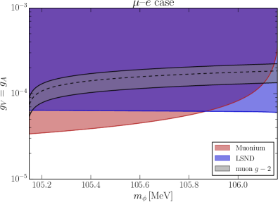
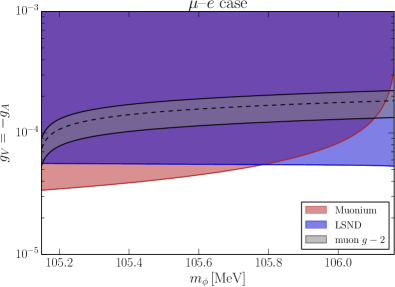
Figure 3: The constraints on the couplings in the $\mu\,\mathchar 45\relax\mathchar 45\relax\,e$ case. The region excluded by the muonium invisible decay and the LSND is covered in red and blue, respectively. The black dashed line corresponds to the central value of the muon $g-2$ anomaly, and the gray region indicates the $1\sigma$ band. The left panel is with $g_{V}=g_{A}$ while the right panel is with $g_{V}=-g_{A}$. Note that only the LSND constraint is (mildly) affected by the relative sign between $g_{V}$ and $g_{A}$. One can see that the whole parameter region favored by the muon $g-2$ is excluded.

The decay of $\phi$ in the detector volume will create a very soft electron and a positron with energies closely following the Michel positron spectrum for the on-shell muon decay. Thus $\phi$ decay will appear as a single energetic $e^{+}$ in that detector. Therefore, one should look for a signature of $\phi$ decays in the sample of neutrino-electron scattering events, $\nu e\to\nu e$, as electron and positron events are nearly identical. The observed spectrum of beam excess events, consistent with the neutrino scattering on electrons at the LSND experiment, is reported in LSND:2001akn . In particular, the experiment observed 49 events in the energy bin $20\,\mathrm{MeV}<E_{e}<22\,\mathrm{MeV}$ with $\cos\theta_{e}>0.9$. Therefore, we can derive a conservative constraint on the coupling, without subtracting $\nu e$ scattering and by requiring that

$$N_{e} =\int_{20\,\mathrm{MeV}}^{22\,\mathrm{MeV}}dE_{e}\int_{0.9}^{1}d\cos\theta_{e}\frac{d^{2}N_{e}}{dE_{e}d\cos\theta_{e}}<49.$$ (28)

If we include the other energy bins and energy spectrum information, the constraint will get stronger, but the above condition is enough for our purpose, to exclude the region relevant for the muon $g-2$. In Fig. 3, we plot the constraint from the muonium invisible decay (23) and the LSND experiment (28), where we take $P(\mu^{+}\to\mathrm{Mu}^{(S=1)})=3/4$ Gninenko:2012nt . As one can see, the whole parameter region that explains the muon $g-2$ is excluded. Our constraint relies on two distinct observables and hence is robust. We have checked that the parameter region $\left\lvert g_{V}\right\rvert\gtrsim\left\lvert g_{A}\right\rvert$ that can explain muon $g-2$ without spoiling the electron $g-2$ measurement is also excluded by the muonium invisible decay and the LSND experiment.

4 $\tau\,\mathchar 45\relax\mathchar 45\relax\,\mu$ case: Beam dump experiments

We now move to the $\tau\,\mathchar 45\relax\mathchar 45\relax\,\mu$ case, for which the considerations are much different from the $e\,\mathchar 45\relax\mathchar 45\relax\,\mu$ case. In this case, high energy beam dump experiments such as CHARM, NuTeV, and SHiP that can produce a sizable amount of $\tau$ can also produce $\phi$, and its subsequent decay at downstream detectors can be observed and used to probe the model. As we will see, although the CHARM and NuTeV experiments do not exclude the parameter region interesting for the muon $g-2$ anomaly, the future SHiP experiment can cover the whole parameter space.

Table 1: Major experiments and parameters for the $\tau-\mu$ case, see details in the text. For comparison, we list the geometric acceptance for the $D_{s}$ production at CHARM and SHiP experiments.

Experiment	$E_{\rm beam}$(GeV)	POT	$D$ (m)	$L$ (m)	$A$ ($m^{2}$)	$\epsilon^{\rm geo}_{\rm acpt}$	Major production
CHARM	400	$2\times 10^{18}$	480	35	3$\times$3	1.3%	EW, $D_{s}$, $\mu$OT
NuTeV	800	$\mu$OT	850	34	$2.54\times 2.54$	$\mathcal{O}$(1)%	$\mu$OT
SHiP	400	$2\times 10^{20}$	60	60	5$\times$10	54%	EW, $D_{s}$, $\mu$OT

4.1 Production mechanism

First, we discuss the production of $\phi$ at beam dump experiments. We focus on high-energy beam dump experiments such as the past CHARM and NuTeV experiments as well as the future SHiP experiment, as high energy is required to produce $\phi$ with its mass $m_{\phi}\sim m_{\tau}$. In these experiments, we notice three ways of producing $\phi$: the direct electroweak process, heavy meson ($D_{s}$ dominant) decay, and high energy muon passing through dense matter, which we may refer to as “muon on target.”

Figure 4: Primary production modes and representative Feynman diagrams for each mode for the $\mu$-$\tau$-flavored scalar $\phi$ at beam dumps.

We show schematically representative diagrams for each production mode in Figure 4. Depending on the detailed beam and detector setup, different mode dominates the detectable $\phi$ fluxes, which we summarize in Table 1. We explain each process in this section.

4.1.1 Direct electroweak production

With a high energy beam, the direct weak interaction production from parton scatterings is one of the primary sources for the $\phi$ flux. The electroweak process is with initial states quark pair colliding to $\phi$ plus lepton pairs, namely, $q\bar{q}\rightarrow\tau^{\mp}\mu^{\pm}\phi^{(*)}$. In the $\sqrt{s}$ energy regime suitable for the beam dumps considered in this study, the main contribution is through the $s$-channel off-shell photon diagram. Given the minimal partonic center of mass energy required here is above $\sim 2m_{\tau}=3.4$ GeV, the parton model works well to describe the production cross section here. We choose MadGraph Alwall:2011uj to simulate the direct weak production cross section and kinematics distributions. A typical Feynman diagram is shown in the left panel of Figure 4.

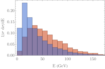
Figure 5: The normalized differential energy distribution from the direct EW production at SHiP experiment. The blue and red distribution are before and after the angular acceptance selection. The geometric acceptance slightly favors higher energy with a signal geometric acceptance efficiency of 42% for SHiP.

Given the center of mass energy of the beam-on-target collisions is around $15-20$ GeV, a partonic center of mass energy above 3.4 GeV corresponds to a sizable $x$ in the parton distribution functions. Hence, $\phi$ productions are typical with small transverse momentum, making the geometric acceptance of near detectors of various experiments sizable. To illustrate a typical energy distribution, we show in Figure 5 the normalized energy distribution of the produced $\phi$, which has very little dependence on the $\phi$ mass in the allowed mass window. We show the distribution at production in blue and the geometrically accepted distribution by the SHiP experiment in red. We can see that geometric selection favors slightly harder $\phi$’s as there is a typical transverse momentum associated with the production. For the case of CHARM and NuTeV, the geometric selection will be further biased towards the high energy part. The production is off-shell photon exchange dominated, given that the massive gauge boson mediated processes (both neutral and charged current) are highly suppressed by $\hat{s}^{2}/m_{W,Z}^{4}$ (and $\hat{s}/m_{W,Z}^{2}$ for the interference). We hence do not include the charged current production in this study.

4.1.2 Heavy meson decay

In typical beam dump experiments, the primary source of $\tau$ is the decay of $D_{s}$ mesons, since kaons and pions do not have enough mass while the decays of other $D$ meson are suppressed by the CKM matrix element. In a similar way, $D_{s}$ mesons can produce $\phi$ through off-shell $\tau$, whose amplitude is diagrammatically given by

$$i\mathcal{M} =\leavevmode\hbox to0pt{\vbox to0pt{\text{[drawing]}}}. \scriptstyle{D^{-}_{s},\,P} \scriptstyle\bar{\nu}_{\tau}{,}\,p_{3} \scriptstyle\mu^{-}{,}\,p_{2} \scriptstyle\phi^{*}{,}\,p_{1} \scriptstyle{D^{-}_{s},\,P} \scriptstyle\bar{\nu}_{\tau}{,}\,p_{3} \scriptstyle\mu^{-}{,}\,p_{2} \scriptstyle\phi^{*}{,}\,p_{1}$$ (29)

The effective Lagrangian relevant for this process is induced from the charged current and is given by

$$\mathcal{L}_{\mathrm{eff}} =-\frac{G_{F}}{\sqrt{2}}V_{cs}f_{D_{s}}(\partial_{\mu}D_{s}^{-})\bar{\tau}\gamma^{\mu}(1-\gamma_{5})\nu_{\tau}+\mathrm{(h.c.)},$$ (30)

where $V_{cs}\simeq 0.95$ is the CKM matrix element and $f_{D_{s}}\simeq 255\,\mathrm{MeV}$ is the $D_{s}$ decay constant Bernard:2000ki ; ALEPH:2002fge . The amplitude is given by

$$i\mathcal{M} =-\frac{G_{F}}{\sqrt{2}}V_{cs}f_{D_{s}}\bar{u}_{\mu}(p_{2})\left(g_{V}+g_{A}\gamma_{5}\right)\frac{\not{p}_{12}+m_{\tau}}{m_{12}^{2}-m_{\tau}^{2}}\not{P}(1-\gamma_{5})u_{\nu_{\tau}}(p_{3}),$$ (31)

where $p_{ij}=p_{i}+p_{j}$ and $m_{ij}^{2}=p_{ij}^{2}$. The decay width follows

$$\Gamma(D_{s}\to\phi\mu\nu_{\tau}) =\frac{1}{256\pi^{3}m_{D_{s}}^{3}}\int_{(m_{\phi}+m_{\mu})^{2}}^{m_{D_{s}}^{2}}dm_{12}^{2}\int_{(m_{23}^{2})_{+}}^{(m_{23}^{2})_{-}}dm_{23}^{2}\left\lvert M\right\rvert^{2},$$ (32)

where

$$(m_{23}^{2})_{\pm} =\left(E_{2}^{*}+E_{3}^{*}\right)^{2}-\left(\sqrt{E_{2}^{*2}-m_{\mu}^{2}}\pm E_{3}^{*}\right)^{2},$$ (33)

with

$$E_{2}^{*}=\frac{1}{2m_{12}}\left(m_{12}^{2}-m_{\phi}^{2}+m_{\mu}^{2}\right),\quad E_{3}^{*}=\frac{1}{2m_{12}}\left(m_{D_{s}}^{2}-m_{12}^{2}\right).$$ (34)

We plot the branching ratio in Figure 6. The branching ratio strongly depends on $m_{\phi}$ due to the phase space suppression. In particular, since $m_{\tau}+m_{\mu}>m_{D_{s}}-m_{\mu}$, the branching ratio vanishes in the large $m_{\phi}$ region.

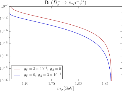
Figure 6: The branching ratio of $D_{s}$ decaying to $\nu_{\tau}\mu\phi$. The red line corresponds to $g_{V}=3\times 10^{-3}$ and $g_{A}=0$, while the blue line to $g_{V}=0$ and $g_{A}=3\times 10^{-3}$. Note that the branching ratio is strongly suppressed due to the phase space in the large $m_{\phi}$ region, and eventually vanishes for $m_{D_{s}}-m_{\mu}<m_{\phi}<m_{\tau}+m_{\mu}$.

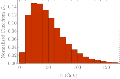
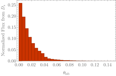
Figure 7: The normalized differential energy distribution and the angular distribution from the $D_{s}$ production at SHiP experiment.

In our numerical computation, we simulate the flux of $\phi$ from $D_{s}$ at the beam dump experiment using the combination Pythia8 Sjostrand:2014zea ; Bierlich:2022pfr and our code. The $D_{s}$ production is driven by the soft-QCD process, which we use Pythia8 to simulate the cross section and kinematics. Then the number of $D_{s}$ produced at the target can be calculated as the product of the PoT, and we calculated the $D_{s}$ production cross section, and then divided by the total inclusive proton target-nucleus cross section of $\sigma_{pN}=10.7$ mb reported in Ref. SHiP:2015vad . We then decay the $D_{s}$ into $\phi+\tau+\mu$ in an approximation that ignores angular correlations (three-body phase space mapping) since we do not expect a strong angular correlation for the scalar decay. In Figure 7 we show the normalized differential energy distribution (left panel) and angular distribution (right panel) at the SHiP experiment to show the typical behavior of $\phi$ from $D_{s}$ production. In the left panel, we can see that the typical energy of scalar produced through $D_{s}$ decay peaks around 30-40 GeV, with a long tail expanding to the hundreds of GeV regime. The spread of the energy distribution provides us access to both short- and long-lifetime regimes. The right panel shows that the $\phi$ production from $D_{s}$ decays does prefer the forward regions along the beam direction, enabling significant effective angular acceptance for the signal. To verify and cross-check our numerical computation, we estimated the $D_{s}$ spectrum based on the differential cross section of $pN\to c\bar{c}X$ and the $D_{s}$ formation rate provided in Alekhin:2015byh , assuming for simplicity that $c$ and $D_{s}$ have the same kinetic energy. We have checked that the constraint derived from this procedure agrees well with our numerical computation.

4.1.3 Muon on target

In beam dump experiments, high-energy muon flux is produced mainly from the decay of mesons, in particular from charged pions and kaons. Once these high-energy muons pass through dense matters, the muons can produce $\phi$ by picking up virtual photons from nuclei, corresponding to the process $\mu N\to\tau\phi N$. We phrase this production mechanism “muon on target,” or $\mu$OT. In the NuTeV experiment, in order to shield high energy muons, there is 850 m of dirt between the meson decay region and the detector, and $\phi$ can be produced from muons passing through this dirt region. In the SHiP experiment, there is $\sim$ 5 m of steel as a beam stop after the target, before the active muon shield by a magnetic field, where $\phi$ can be produced.

The flux of $\phi$ at the detector produced by the $\mu$OT is estimated as

$$\Phi_{\phi}(E_{\phi}) =\int dE\,\Phi_{\mu}(E)\int_{0}^{l_{\mathrm{max}}}dl\,n_{A}\int_{0}^{\theta_{\mathrm{det}}(l)}d\theta_{\phi}\sin\theta_{\phi}\frac{d^{2}\sigma}{dE_{\phi}d\cos\theta_{\phi}}(E_{l},E_{\phi}),$$ (35)

where $\Phi_{\mu}(E)$ is the initial muon flux, $l_{\mathrm{max}}=\mathrm{min}[l_{\mathrm{shield}},l_{\mathrm{stop}}(E)]$ with $l_{\mathrm{shield}}$ the length of the shield and $l_{\mathrm{stop}}(E)$ the length at which the shield stops a muon with initial energy $E$, $n_{A}$ is the number density of the target nuclei, $E_{l}=E_{l}(E)$ is the muon energy at the length $l$ with $E_{0}(E)=E$, $E_{\phi}$ is the energy of the produced $\phi$, $\theta_{\phi}$ is the angle of the produced $\phi$, and $\theta_{\mathrm{det}}(l)$ is the angle between the interaction point and the detector which we specify below. We estimate the differential cross section $d^{2}\sigma/dE_{\phi}d\cos\theta_{\phi}$ based on the equivalent photon approximation (EPA) following Bjorken:2009mm (see App. A.3 for more details). By changing the integration variable from $l$ to $E_{l}$, we can rewrite the above equation as

$$\Phi_{\phi}(E_{\phi}) =\int dE\,\Phi_{\mu}(E)\int_{E_{\mathrm{min}}}^{E}dE_{l}\,\frac{n_{A}}{-dE/dl}\int_{0}^{\theta_{\mathrm{det}}(l(E,E_{l}))}d\theta_{\phi}\sin\theta_{\phi}\frac{d^{2}\sigma}{dE_{\phi}d\cos\theta_{\phi}}(E_{l},E_{\phi}),$$ (36)

where

$$l(E,E_{l})=\int_{E_{l}}^{E}\frac{dE_{l}}{-dE/dl}.$$ (37)

If a muon stops inside the shield $E_{\mathrm{min}}=0$, otherwise, $E_{\mathrm{min}}$ is the energy of the muon at the end of the shield. We read off the stopping power of muon, $-dE/dl$, from ParticleDataGroup:2020ssz . The angular acceptance is essential for the NuTeV experiment in which the detector is located far from the muon production (i.e. the meson decay) region, and the angular acceptance is of order $10^{-2}\,\mathchar 45\relax\mathchar 45\relax\,10^{-3}$.

NuTeV provides the (anti-)neutrino flux per $10^{6}$ POT in NuTeV:2005wsg , and they collected $1.13\times 10^{18}$ POT for positive meson mode and $1.41\times 10^{18}$ POT for negative meson mode. Recognizing that the high energy region of this flux dominantly comes from Kaon decays where muon mass is less important, we may estimate the muon flux simply as $\Phi_{\mu^{+}}=\Phi_{\nu}$ and $\Phi_{\mu^{-}}=\Phi_{\bar{\nu}}$. The shield length of NuTeV is $l_{\mathrm{shield}}=850\,\mathrm{m}$. We take the mass density of the shield as $\rho_{A}=2.7\,\mathrm{g}/\mathrm{cm}^{3}$ which is the standard crust density. We assume for simplicity that the shield is solely composed of Si (which is the dominant component of the Earth), from which we obtain in $n_{A}\simeq 5.8\times 10^{22}\,\mathrm{cm}^{-3}$. In this case, we can simply set $E_{\mathrm{min}}=0$ as even the highest energy muon at NuTeV is well stopped by the shield, as it should be. The fiducial volume of the decay channel region is $2.54\,\mathrm{m}\times 2.54\,\mathrm{m}\times 34\,\mathrm{m}$ NuTeV:2000ehk . Since the detector is right behind the shield, we have

$$\theta_{\mathrm{det}}(l)=\frac{1.27\,\mathrm{m}}{850\,\mathrm{m}-l}.$$ (38)

Note that the (anti-)neutrino flux in NuTeV:2005wsg is normalized by $3\,\mathrm{m}\times 3\,\mathrm{m}$ which is the area of the Lab E detector, and thus, we normalize our estimation of the muon flux by $2.54^{2}/3^{2}$ to be conservative. With this information and Eq. (36) we can estimate the flux of $\phi$ at NuTeV.

SHiP provides their expected muon flux in SHiP:2020hyy , and we use it for our study, with the total number of $2\times 10^{20}$ POT assumed. The SHiP configuration is described in SHiP:2015vad . After the target, there is 5 m of ironic hadron absorber. Then there is 48 m of active muon shield by magnetic fields, followed by 10 m of $\nu_{\tau}$ detector. After the $\nu_{\tau}$ detector there exists $l_{\mathrm{det}}=64\,\mathrm{m}$ of decay volume followed by detectors. In our case, the muon flux produced at the target goes through the hadronic absorber and produces $\phi$ before shielded by the active magnetic field. Therefore we take $l_{\mathrm{shield}}=5\,\mathrm{m}$. The produced $\phi$ travels towards the detector and decays in the decay volume, leaving signals in the detector. We take the iron mass density $\rho_{A}=7.8\,\mathrm{g}/\mathrm{cm}^{3}$ which results in $n_{A}=8.4\times 10^{22}\,\mathrm{cm}^{-3}$. In this case, the muon energy loss inside the hadron absorber is $\sim 10\,\mathrm{GeV}$ which is small compared to the initial muon energy. Therefore we may simply ignore the muon energy loss inside the hadron absorber. The formula is then simplified as

$$\Phi_{\phi}(E_{\phi}) =l_{\mathrm{shield}}n_{A}\int dE\,\Phi_{\mu}(E)\int_{0}^{\theta_{\mathrm{det}}}d\theta_{\phi}\sin\theta_{\phi}\frac{d^{2}\sigma}{dE_{\phi}d\cos\theta_{\phi}}(E,E_{\phi}),$$ (39)

where we take $\theta_{\mathrm{det}}=(10+5)/4/(48+10+64)\simeq 0.031$. We have checked that, as long as $\theta_{\mathrm{det}}\gtrsim 0.02$, the angular acceptance does not affect the flux of $\phi$.

In principle, CHARM can also produce $\phi$ from the $\mu$OT. However, we could not find an appropriate reference to estimate the flux of $\mu$ that passes through the dirt region between the production point and the detector. Moreover, the $\mu$OT constraint of CHARM is expected to be at most comparable to NuTeV and is well above the couplings relevant for the muon $g-2$ anomaly. Therefore we do not consider the $\mu$OT production of CHARM in this study.

4.2 Constraints and future prospects

We now derive the constraints on the couplings from the CHARM and NuTeV experiments, and the future sensitivity of the SHiP experiment. As discussed above, in these experiments, $\phi$ is generated by the direct electroweak production, the $D_{s}$ decay, and the $\mu$OT processes. After production, a fraction of them decay inside the detector and can be identified as signals. The event number is estimated as

$$N_{\mu X} =\int dE_{\phi}\,\Phi_{\phi}(E_{\phi})\times\frac{l_{\mathrm{det}}}{\gamma\beta c\tau_{\phi}},\quad\frac{1}{\gamma\beta}=\left(\frac{E_{\phi}^{2}}{m_{\phi}^{2}}-1\right)^{-1/2},$$ (40)

where we assume that the decay length of $\phi$ satisfies $\gamma\beta c\tau_{\phi}\gg l_{\mathrm{det}}$. In the $\tau\,\mathchar 45\relax\mathchar 45\relax\,\mu$ case the computation of $\phi$’s decay rate is more involved than the $\mu\,\mathchar 45\relax\mathchar 45\relax\,e$ case. In SM, the branching ratio of $\tau^{-}\to\mu^{-}\bar{\nu}_{\mu}\nu_{\tau}$ is around 17 %. Therefore, we estimate the decay rate of $\phi$ by assuming that it shares the same branching ratio 17 % for the channel $\phi\rightarrow\mu^{-}\mu^{+}\nu_{\mu}\bar{\nu}_{\tau}$, whose decay width is given by replacing $\mu\to\tau$ and $e\to\mu$ in Eq. (14). The intermediate $\tau$ is indeed close to on-shell as the mass difference between $\tau$ and $\phi$ is small, which makes our estimation reasonable. Note that the decay product of $\phi$ always contains at least one muon, irrespective of the decay mode of the off-shell $\tau$. For this reason, we denote the event number as $N_{\mu X}$ with $X$ representing the decay product of the off-shell $\tau$. In Figure 8, we plot the decay length of $\phi$ as a function of $m_{\phi}$ estimated in this way. The detector configurations are summarized in Table 1.

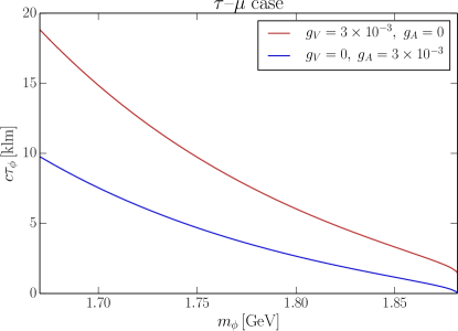
Figure 8: The decay length of $\phi$ in the $\tau-\mu$ case. The red line corresponds to $g_{V}=3\times 10^{-3}$ and $g_{A}=0$, while the blue line does to $g_{V}=0$ and $g_{A}=3\times 10^{-3}$.

In order to derive the constraint from NuTeV, we use the analysis in NuTeV:2001ndo . The NuTeV collaboration detected three $\mu\mu$ events in the decay channel in this analysis. This is significantly more than the expected background, and the origin of these events is still not clear. In the current paper, we use the CLs method to derive the 95% C.L. exclusion on the number of signal events in the $\mu\mu$ channel (with the $\mu\mu\nu\bar{\nu}$ branching fraction of $17\%$) i.e.,

$$N_{\mu X}(\mathrm{NuTeV})<46,$$ (41)

to estimate the constraint. Similarly, for the CHARM experiment in the dilepton plus missing energy channel CHARM:1985nku , 2 events were observed with $1.4\pm 0.4$ expected background. Hence we have

$$N_{\mu X}(\mathrm{CHARM})<14.$$ (42)

For the SHiP experiment, as an estimation of its sensitivity, we simply assume that our event is background-free. We then draw the sensitivity line of the SHiP experiment by requiring that

$$N_{\mu X}(\mathrm{SHiP})<3.0.$$ (43)

Here we assume all decay channels of $\phi$ can be detected at SHiP experiment with negligible background.

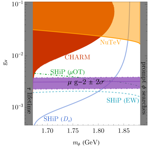
Figure 9: The existing constraint and projection sensitives in the $g_{V}-m_{\phi}$ plane for different experiments.

We summarize the constraints on $g_{V}$ as functions of $m_{\phi}$ in Figure 9. The purple region is the $2\sigma$ parameter space for the muon $g-2$ anomaly. The red and blue regions are covered by the $D_{s}^{\pm}$ decay at the CHARM and SHiP, respectively. The green region can be probed from the SHiP electroweak production channel. The orange and blue lines are from the $\mu$OT at NuTeV and SHiP. For the three production mechanisms at SHiP, the electroweak production dominates for larger $m_{\phi}$ while $D_{s}^{\pm}$ decay wins for smaller $m_{\phi}$. A large $m_{\phi}$ suppresses the phase space of the $D_{s}$ decay as seen in Figure 6. On the other hand, the electroweak production is insensitive to the change of $m_{\phi}$ within the range of our interest. The event number increases as $m_{\phi}$ increases since a larger $m_{\phi}$ leads to a smaller decay length that enhances the decay probability of $\phi$ inside the detector. Here we show the projected sensitivities from the three production mechanisms separately, but of course, we observe the sum of them in reality, which strengthens our projection.

We can see that CHARM and NuTeV cannot exclude the parameter region that explains the muon $g-2$ anomaly, while the future SHiP experiment covers the whole parameter space. In other words, muon $g-2$ provides the most superior probe of this model, compared to the sensitivity of all the existing beam dump experiments. Aside from the big increase in intensity, an essential advantage of the SHiP is that the detector will be placed much closer to the beam dump target than CHARM and NuTeV, thus avoiding suppression from angular acceptance.

Before closing this section, we may comment on the $\tau$ lepton flavor violation (LFV) search at Belle II. In Tenchini:2020njf , Belle II looks for an LFV decay $\tau\to e\alpha$ with $\alpha$ a new particle by studying the spectrum of the electron in the $\tau$ pseudo-rest frame constructed from the decay products of the other $\tau$, following the strategy of ARGUS experiment ARGUS:1995bjh . A similar technique is applicable to our $\tau\,\mathchar 45\relax\mathchar 45\relax\,\mu$ case as the new $\tau$ decay mode prefers $\phi$ to be close to on-shell, which results in a peak-like structure of the muon spectrum in the $\tau$ (pseudo-)rest frame. Our estimation indicates that the current limit is not strong enough to probe the parameter region relevant for the muon $g-2$, mainly because the inferred signal acceptance rate is low, but it would be interesting to study future Belle II sensitivity to this channel in more detail.

5 Summary

In this paper, we studied the phenomenology of a complex scalar field $\phi$ that couples dominantly to $\mu$ and either $e$ or $\tau$, motivated by the muon $g-2$ anomaly. We focused on the mass range $\left\lvert m_{l}-m_{\mu}\right\rvert<m_{\phi}<m_{l}+m_{\mu}$ where $l=e$ or $\tau$. Despite the limited parameter region, this mass range provides us with interesting phenomenological signatures. The upper bound prohibits the two body-decay $\phi\to l+\mu$, making $\phi$ accidentally long-lived, while the lower bound prohibits $\tau\to\phi+\mu$ and $\mu\to\phi+e$, avoiding stringent constraints on the couplings from the lepton flavor violation experiments.

In the $\mu\,\mathchar 45\relax\mathchar 45\relax\,e$ case, we found that the whole parameter region that explains the muon $g-2$ anomaly is excluded by the MuLan and LSND experiments. Our key observation is that, although the mass range $m_{\mu}-m_{e}<m_{\phi}<m_{\mu}+m_{e}$ prohibits the decay of free muon $\mu\to\phi+e$, it still allows the decay of muonium (the bound state of $\mu^{+}$ and $e^{-}$) into $\phi$ and photon. The MuLan experiment performed a dedicated measurement of the muon lifetime with two different materials, one with the muonium formation and the other without, from which one can derive a constraint on the muonium invisible decay rate. More interestingly, $\phi$ can be produced from the muonium decay in neutrino experiments that use stopped $\mu^{+}$, such as the LSND experiment. A fraction of the produced $\phi$ decays inside the LSND detector, from which we constrained the coupling between $\phi$ and the leptons.

In the $\mu\,\mathchar 45\relax\mathchar 45\relax\,\tau$ case, we studied both the past and future high-energy beam dump experiments, CHARM, NuTeV, and SHiP. We found that, although CHARM and NuTeV do not exclude the parameter region relevant for the muon $g-2$ anomaly, the future SHiP experiment can cover the entire region. In the $\mu\,\mathchar 45\relax\mathchar 45\relax\,\tau$ case, $\phi$ can be produced from three distinct processes, the decay of $D_{s}$ meson, the electroweak interaction and the high-energy muons passing through dense matter. In particular, we pointed out that the NuTeV experiment can be interpreted as a “muon on target” experiment as the muons produce $\phi$ while passing through 850 m of dirt between the meson decay region and the detector. This channel covers the large mass end of $m_{\phi}$ that is not covered by the $D_{s}$ decay due to the phase space suppression. Although SHiP can also be interpreted as the muon beam dump experiment, the $D_{s}$ decay and the electroweak production are more efficient as the muon on target is limited by the length of the absorber.

Throughout this paper, we focused on the flavor off-diagonal couplings of $\phi$ and ignored the flavor diagonal couplings by assigning the global lepton U(1) charge to $\phi$. This global symmetry is broken due to the neutrino oscillation, but the effect is suppressed by the small neutrino mass (difference) and hence is negligible. Thus, as long as a UV model does not introduce any additional breaking of this (approximate) symmetry, our assumption that $\phi$ has only the flavor off-diagonal couplings is justified.

Beyond detecting the decays of $\phi$, we can also consider the scattering of $\phi$ with detector materials. The signal and background considerations will require more detailed simulations of the detector performance, which we save for future work. To close up, we would like to point out that the longevity mass windows, identified in this work, can also exist for the coupling with quarks. For example, a scalar $\phi$ coupled to $s-d$ current in the $m_{K}-m_{\pi}<m_{\phi}<m_{K}+m_{\pi}$ mass window will lead to long lifetimes even for a sizable coupling, as the two-body decays to mesons will be forbidden. Such models will lead to intricate phenomenology of $\phi$ production and decay, and for certain mass ranges may add additional rare kaon decay modes, such as $K_{L}\to\phi\gamma\gamma$ that may compete with the SM $K_{L}\to\nu\bar{\nu}\pi^{0}\to\nu\bar{\nu}\gamma\gamma$ decay (see e.g. Hostert:2020gou ). An in-depth analysis of the long-lived scalars coupled with quarks may deserve further studies.

Appendix A Computational details

A.1 $\phi$ decay rate

In this appendix we explain the computation of $\phi$ decay rate that is crucial for our study in the main text. We focus on the $l=e$ case in the following. As we explained in the main text, the decay rate in the $l=\tau$ case can be reasonably estimated from the $l=e$ case by replacing $\mu\to\tau$ and $e\to\mu$ in the final result and rescaling by the branching ratio of $\tau$.

Since $\mu$ almost always decays into $e\nu_{\mu}\nu_{e}$, we focus on the decay $\phi\to e^{+}e^{-}\nu_{\mu}\bar{\nu}_{e}$ mediated by muon. The amplitude is diagrammatically given by

$$i\mathcal{M}=\leavevmode\hbox to6.67pt{\vbox to6.67pt{\text{[drawing]}}}, {\scriptstyle\phi,\,P} {\scriptstyle e^{+},\,p_{1}} {\scriptstyle e^{-},\,p_{2}} {\scriptstyle\nu_{\mu},\,p_{3}} {\scriptstyle\bar{\nu}_{e},\,p_{4}} {\scriptstyle\phi,\,P} {\scriptstyle e^{+},\,p_{1}} {\scriptstyle e^{-},\,p_{2}} {\scriptstyle\nu_{\mu},\,p_{3}} {\scriptstyle\bar{\nu}_{e},\,p_{4}}$$ (44)

where the black dot indicates the 4-fermi interaction

$$\mathcal{L}=-\frac{G_{F}}{\sqrt{2}}\left[\bar{\nu}_{\mu}\gamma_{\alpha}(1-\gamma_{5})\mu\right]\left[\bar{e}\gamma^{\alpha}(1-\gamma_{5})\nu_{e}\right],$$ (45)

and the arrow indicates the flow of the muon number. The amplitude squared is given by

$$\left\lvert\mathcal{M}\right\rvert^{2} =\frac{128G_{F}^{2}}{(p_{234}^{2}-m_{\mu}^{2})^{2}}(p_{2}\cdot p_{3})p_{4}^{\alpha}$$

$$\times\left[\left\lvert g_{V}+g_{A}\right\rvert^{2}\left(2(p_{1}\cdot p_{234})p_{234\alpha}-p_{234}^{2}p_{1\alpha}\right)+\left\lvert g_{V}-g_{A}\right\rvert^{2}m_{\mu}^{2}p_{1\alpha}-2(\left\lvert g_{V}\right\rvert^{2}-\left\lvert g_{A}\right\rvert^{2})m_{e}m_{\mu}p_{234\alpha}\right],$$ (46)

where we use the notation $p_{ij}=p_{i}+p_{j}$ and $p_{ijk}=p_{i}+p_{j}+p_{k}$, and we take the spin sum of the final particles. The decay rate is given by

$$\Gamma_{\phi}=\frac{1}{2m_{\phi}}\int d\Phi_{4}\left\lvert M\right\rvert^{2}.$$ (47)

We may decompose the phase space integral as

$$\int d\Phi_{4} =\int_{m_{e}^{2}}^{(m_{\phi}-m_{e})^{2}}\frac{d\bar{m}_{\mu}^{2}}{2\pi}\int d\Phi_{1;234}\int_{0}^{(\bar{m}_{\mu}-m_{e})^{2}}\frac{d\bar{m}_{\nu\nu}^{2}}{2\pi}\int d\Phi_{2;34}\int d\Phi_{34},$$ (48)

where

$$\int d\Phi_{1;234} =\int\frac{d^{3}p_{1}}{(2\pi)^{3}2E_{1}}\int\frac{d^{3}p_{234}}{(2\pi)^{3}2\bar{E}_{234}}(2\pi)^{4}\delta^{(4)}(P-p_{1}-p_{234}),$$ (49)

$$\int d\Phi_{2;34} =\int\frac{d^{3}p_{2}}{(2\pi)^{3}2E_{2}}\int\frac{d^{3}p_{34}}{(2\pi)^{3}2\bar{E}_{34}}(2\pi)^{4}\delta^{(4)}(p_{234}-p_{2}-p_{34}),$$ (50)

$$\int d\Phi_{34} =\int\frac{d^{3}p_{3}}{(2\pi)^{3}2p_{3}}\int\frac{d^{3}p_{4}}{(2\pi)^{3}2p_{4}}(2\pi)^{4}\delta^{(4)}(p_{34}-p_{3}-p_{4}),$$ (51)

and we denote $p_{234}^{2}=\bar{m}_{\mu}^{2}$, $p_{34}^{2}=\bar{m}_{\nu\nu}^{2}$, $\bar{E}_{234}^{2}={\left\lvert\vec{p}_{234}\right\rvert^{2}+\bar{m}_{\mu}^{2}}$, and $\bar{E}_{34}^{2}={\left\lvert\vec{p}_{34}\right\rvert^{2}+\bar{m}_{\nu\nu}^{2}}$. We first note that the matrix element squared depends on $p_{3}$ and $p_{4}$ only through the combination $p_{3}^{\alpha}p_{4}^{\beta}$. After the phase space integral we find that

$$\int d\Phi_{34}\,p_{3}^{\alpha}p_{4}^{\beta}=\frac{1}{96\pi}\left(\eta^{\alpha\beta}\bar{m}_{\nu\nu}^{2}+2p_{34}^{\alpha}p_{34}^{\beta}\right),$$ (52)

by evaluating the integral in the $p_{34}$-rest frame and exploiting the Lorentz invariance. Therefore we obtain

$$\int d\Phi_{2;34}\int d\Phi_{3;4}(p_{2}\cdot p_{3})p_{4}^{\alpha} =\frac{1}{96\pi}\int d\Phi_{2;34}\left[p_{2}^{\alpha}\bar{m}_{\nu\nu}^{2}+2(p_{2}\cdot p_{34})p_{34}^{\alpha}\right]=\frac{I_{1}(\bar{m}_{\mu},\bar{m}_{\nu\nu})}{1536\pi^{2}}p_{234}^{\alpha},$$ (53)

where we use the Lorentz invariance in the last line. By working in the $p_{234}$-rest frame, we find that

$$I_{1} =\left[1+\frac{\bar{m}_{\nu\nu}^{2}-2m_{e}^{2}}{\bar{m}_{\mu}^{2}}+\frac{m_{e}^{4}+m_{e}^{2}\bar{m}_{\nu\nu}^{2}-2\bar{m}_{\nu\nu}^{4}}{\bar{m}_{\mu}^{4}}\right]\sqrt{\left(\bar{m}_{\mu}^{2}-\bar{m}_{\nu\nu}^{2}\right)^{2}-2m_{e}^{2}(\bar{m}_{\mu}^{2}+\bar{m}_{\nu\nu}^{2})+m_{e}^{4}}.$$ (54)

By substituting this to Eq. (47) and performing the angular integral, we obtain Eq. (14).

A.2 Muonium decay rate

Since we take $m_{\mu}-m_{e}<m_{\phi}<m_{\mu}+m_{e}$, muonium decay to $\phi$ and $\gamma$ is kinematically allowed. We compute the branching ratio of this process here. The muonium state is written as (see e.g. Peskin:1995ev )

$$\left|\mathrm{Mu}\right\rangle=\sqrt{2E_{\mathrm{Mu}}}\int\frac{d^{3}k}{(2\pi)^{3}}\tilde{\psi}(\vec{k})\frac{1}{\sqrt{2m_{\mu}}}\frac{1}{\sqrt{2m_{e}}}\lvert\mu;\vec{k}\rangle\otimes\lvert e;-\vec{k}\rangle,$$ (55)

where $E_{\mathrm{Mu}}$ is the energy of the muonium and $\tilde{\psi}$ is the (momentum-space) muonium wavefunction. The amplitude is then given by

$$\mathcal{M}(\mathrm{Mu}\to\phi\gamma)=\sqrt{2E_{\mathrm{Mu}}}\int\frac{d^{3}k}{(2\pi)^{3}}\tilde{\psi}(\vec{k})\frac{1}{\sqrt{2m_{\mu}}}\frac{1}{\sqrt{2m_{e}}}\mathcal{M}_{\mathrm{free}}(\mu e\to\phi\gamma),$$ (56)

where $\mathcal{M}_{\mathrm{free}}$ is the matrix element between free particles. We work in the muonium rest frame. Inside muonium both muon and electron are non-relativistic ($v\sim\alpha\ll 1$), and thus we work only on the leading order in the non-relativistic limit, dropping $\vec{k}$ dependence of $\mathcal{M}_{\mathrm{free}}$. We also work in the limit $m_{e}/m_{\mu}\ll 1$ and keep only the leading order terms. We then obtain

$$\Gamma(\mathrm{Mu}\to\phi\gamma) =\frac{|\vec{p}|\left\lvert\psi(0)\right\rvert^{2}}{64\pi^{2}m_{\mu}^{2}m_{e}}\int d\Omega_{2}\left\lvert\mathcal{M}_{\mathrm{free}}(\mu e\to\phi\gamma)\right\rvert^{2},$$ (57)

where $\vec{p}$ is the momentum of the final state photon, $\psi(0)$ is the coordinate-space muonium wavefunction at the origin, and we ignore the binding energy which is of order $\alpha^{2}m_{e}$. Note that this can be written as

$$\Gamma(\mathrm{Mu}\to\phi\gamma) =\left\lvert\psi(0)\right\rvert^{2}\times\sigma_{\mathrm{free}}v(\mu e\to\phi\gamma).$$ (58)

We may parametrize $m_{\phi}$ as

$$m_{\phi}=m_{\mu}+xm_{e},$$ (59)

where $-1<x<1$ in the case of our interest. The kinematics then tells us that

$$\left\lvert\vec{p}\right\rvert\simeq m_{e}(1-x),\quad E_{\phi}\simeq m_{\mu}+xm_{e}.$$ (60)

If we take the ground state muonium, the wavefunction at the origin is given by

$$\left\lvert\psi(0)\right\rvert^{2}=\frac{\alpha^{3}m_{e}^{3}}{\pi}.$$ (61)

We thus obtain

$$\Gamma(\mathrm{Mu}\to\phi\gamma) =\frac{(1-x)\alpha^{3}}{64\pi^{3}}\frac{m_{e}^{3}}{m_{\mu}^{2}}\int d\Omega_{2}\left\lvert\mathcal{M}_{\mathrm{free}}(\mu e\to\phi\gamma)\right\rvert^{2}.$$ (62)

Now comes the evaluation of the matrix element squared in the non-relativistic limit. For this it is convenient to work in the Dirac representation

$$\gamma^{0}=\begin{pmatrix}1&0\\ 0&-1\end{pmatrix},\quad\gamma^{i}=\begin{pmatrix}0&\sigma^{i}\\ -\sigma^{i}&0\end{pmatrix},\quad\gamma_{5}=\begin{pmatrix}0&1\\ 1&0\end{pmatrix}.$$ (63)

In this representation the spinors in the non-relativistic limit are given by

$$u_{e}=\sqrt{2m_{e}}\begin{pmatrix}\chi_{e^{-}}\\ 0\end{pmatrix},\quad v_{\mu}=\sqrt{2m_{\mu}}\begin{pmatrix}0\\ \chi_{\mu^{+}}\end{pmatrix}.$$ (64)

We also note that

$$(p_{\mu}-p_{\phi})^{2}-m_{e}^{2}\simeq-2(1-x)m_{e}^{2},\quad(p_{\mu}-p_{\gamma})^{2}-m_{\mu}^{2}\simeq-2m_{\mu}m_{e}(1-x).$$ (65)

We thus obtain after some computation that

$$\mathcal{M}_{\mathrm{free}}\simeq e\sqrt{\frac{m_{\mu}}{m_{e}}}\left[g_{V}n^{i}+ig_{A}\epsilon^{ijk}\hat{p}^{j}n^{k}\right]\left(\epsilon^{i}_{\lambda}\right)^{*},\quad\hat{p}^{i}=\frac{p^{i}}{|\vec{p}|},\quad n^{i}=\chi_{\mu^{+}}^{\dagger}\sigma^{i}\chi_{e^{-}},$$ (66)

where $\vec{\epsilon}_{\lambda}$ is the polarization vector of the photon with its polarization $\lambda$. We note in passing that only the $t$-channel process gives a finite contribution above. After taking the polarization sum of the photon, the matrix element squared is given by

$$\sum_{\lambda}\left\lvert M_{\mathrm{free}}\right\rvert^{2}=e^{2}\frac{m_{\mu}}{m_{e}}\left(\left\lvert g_{V}\right\rvert^{2}+\left\lvert g_{A}\right\rvert^{2}\right)\left(\left\lvert\vec{n}\right\rvert^{2}-\left\lvert\hat{p}\cdot\vec{n}\right\rvert^{2}\right).$$ (67)

The direction of $\vec{p}$ is unrelated to $\vec{n}$, and thus after the solid angle integral we obtain

$$\Gamma(\mathrm{Mu}\to\phi^{*}\gamma) =\frac{1-x}{6\pi}\frac{\alpha^{4}m_{e}^{2}}{m_{\mu}}\left(\left\lvert g_{V}\right\rvert^{2}+\left\lvert g_{A}\right\rvert^{2}\right)\left\lvert\vec{n}\right\rvert^{2}.$$ (68)

In order to evaluate $\left\lvert\vec{n}\right\rvert^{2}$, we may note that

$$\chi_{\mu^{+}} =\begin{pmatrix}0\\ 1\end{pmatrix}~{}~{}\mathrm{for}~{}~{}\mu^{+}:|\uparrow\rangle,\quad\chi_{\mu^{+}}=\begin{pmatrix}-1\\ 0\end{pmatrix}~{}~{}\mathrm{for}~{}~{}\mu^{+}:|\downarrow\rangle,$$ (69)

since $\mu^{+}$ is anti-particle. It then follows that $\left\lvert\vec{n}\right\rvert^{2}=2$ for triplet and $\left\lvert\vec{n}\right\rvert^{2}=0$ for singlet. We thus have

$$\Gamma\left(\mathrm{Mu}^{(S=1)}\to\phi^{*}\gamma\right) =\frac{1-x}{3\pi}\frac{\alpha^{4}m_{e}^{2}}{m_{\mu}}\left(\left\lvert g_{V}\right\rvert^{2}+\left\lvert g_{A}\right\rvert^{2}\right),\quad\Gamma\left(\mathrm{Mu}^{(S=0)}\to\phi^{*}\gamma\right)=0,$$ (70)

reproducing Eqs. (20) and (21) in the main text.

A.3 Equivalent photon approximation

In this subsection we explain the EPA that we used to estimate the flux of $\phi$ in the muon beam dump. Following Bjorken:2009mm , we approximate the scattering cross section of $\mu(p)N(P_{i})\to\tau(p^{\prime})\phi(k)N(P_{f})$ as

$$\frac{d\sigma(p+P_{i}\to p^{\prime}+k+P_{f})}{dE_{\phi}d\cos\theta_{\phi}}=\frac{\alpha\chi}{\pi}\frac{E_{\mu}x\beta_{\phi}}{1-x}\left.\frac{d\sigma(p+q\to p^{\prime}+k)}{d(p\cdot k)}\right|_{t=t_{\mathrm{min}}},$$ (71)

where

$$q=P_{i}-P_{f},\quad x=E_{\phi}/E_{\mu},\quad t=-q^{2},\quad\beta_{\phi}=\sqrt{1-\frac{m_{\phi}^{2}}{E_{\mu}^{2}}},$$ (72)

and $\theta_{\phi}$ is the scattering angle between the initial muon and the final $\phi$ in the lab frame. Here $\sigma(p+q\to p^{\prime}+k)$ represents the cross section of $\mu(p)\gamma(q)\to\tau(p^{\prime})\phi(k)$ with $\gamma$ indicating the virtual photon created by the nucleus. The EPA assumes that

$$m_{\tau},m_{\phi},m_{\mu},\left\lvert\vec{q}\right\rvert\ll E_{\mu},\quad\left\lvert\vec{q}\right\rvert\ll m_{A},\quad\theta_{\phi}\ll 1,$$ (73)

where $m_{A}$ is the mass of the target nucleus. The above formula assumes that $\vec{q}$ is collinear with $\vec{k}-\vec{p}$ such that the photon virtuality $t$ takes its minimum $t_{\mathrm{min}}$ (note that $m_{\tau}^{2}=(p-k+q)^{2}$ is fixed). To the leading order in this kinematics, we obtain in the lab frame (where $P_{i}=(m_{A},0,0,0)$)

$$q^{0} \simeq-\frac{\left\lvert\vec{q}\right\rvert^{2}}{2m_{A}}\ll\left\lvert\vec{q}\right\rvert,\quad\left\lvert\vec{q}\right\rvert\simeq-\frac{u_{2}-m_{\tau}^{2}}{2E_{\mu}(1-x)},\quad t_{\mathrm{min}}\simeq\left(\frac{u_{2}-m_{\tau}^{2}}{2E_{\mu}(1-x)}\right)^{2},$$ (74)

$$u_{2} =(p-k)^{2}\simeq-E_{\mu}^{2}x\theta_{\phi}^{2}-\frac{1-x}{x}m_{\phi}^{2}+(1-x)m_{\mu}^{2},$$ (75)

$$s_{2} =(p+q)^{2}\simeq m_{\mu}^{2}-\frac{u_{2}-m_{\tau}^{2}}{1-x},\quad t_{2}=m_{\phi}^{2}+\frac{x(u_{2}-m_{\tau}^{2})}{1-x},$$ (76)

where the quantities with the subscript $2$ indicate the Mandelstam variables of $\mu\gamma\to\tau\phi$. The form factor is given by

$$\chi=\int_{t_{\mathrm{min}}}^{t_{\mathrm{max}}}dt\frac{t-t_{\mathrm{min}}}{t^{2}}F^{2}(t),\quad F^{2}(t)=\frac{Z^{2}}{(1+t/d)^{2}},$$ (77)

with $d=0.164\,\mathrm{GeV}^{2}A^{-2/3}$ and $t_{\mathrm{max}}=m_{\phi}^{2}$. We ignore the atomic form factor since that is irrelevant for our energy scale. Finally the differential cross section of $\mu\gamma\to\tau\phi$ is given by

$$\frac{d\sigma(p+q\to p^{\prime}+k)}{d(p\cdot k)}=2\frac{d\sigma}{dt_{2}}\simeq\frac{\left\lvert\bar{\mathcal{M}}\right\rvert^{2}}{8\pi s_{2}^{2}},$$ (78)

where

$$\left\lvert\bar{\mathcal{M}}\right\rvert^{2}=-\frac{e^{2}}{4}\mathrm{Tr} \left[\left(\not{p}^{\prime}+m_{\tau}\right)\left(\frac{(g_{V}^{*}-g_{A}^{*}\gamma_{5})(\not{p}+\not{q}+m_{\mu})}{s_{2}-m_{\mu}^{2}}\gamma^{\alpha}+\gamma^{\alpha}\frac{(\not{p}-\not{k}+m_{\tau})(g_{V}^{*}-g_{A}^{*}\gamma_{5})}{u_{2}-m_{\tau}^{2}}\right)\right.$$

$$\left.\times\left(\not{p}+m_{\mu}\right)\left(\gamma_{\alpha}\frac{(\not{p}+\not{q}+m_{\mu})(g_{V}+g_{A}\gamma_{5})}{s_{2}-m_{\mu}^{2}}+\frac{(g_{V}+g_{A}\gamma_{5})(\not{p}-\not{k}+m_{\tau})}{u_{2}-m_{\tau}^{2}}\gamma_{\alpha}\right)\right].$$ (79)

We set $t_{\mathrm{min}}=0$ in the evaluation of this expression.

References

- (1) S. Davidson, B. Echenard, R.H. Bernstein, J. Heeck and D.G. Hitlin, Charged Lepton Flavor Violation, 2209.00142.
- (2) MEG II collaboration, MEG II experiment status and prospect, PoS NuFact2021 (2022) 120 [2201.08200].
- (3) MEG II collaboration, Towards a New →e Search with the MEG II Experiment: From Design to Commissioning, Universe 7 (2021) 466.
- (4) Mu2e collaboration, Mu2e Technical Design Report, 1501.05241.
- (5) Mu3e collaboration, The Mu3e Experiment, in 2022 Snowmass Summer Study, 4, 2022 [2204.00001].
- (6) COMET collaboration, COMET Phase-I Technical Design Report, PTEP 2020 (2020) 033C01 [1812.09018].
- (7) Belle-II collaboration, The Belle II Physics Book, PTEP 2019 (2019) 123C01 [1808.10567].
- (8) Belle collaboration, Physics Achievements from the Belle Experiment, PTEP 2012 (2012) 04D001 [1212.5342].
- (9) BaBar collaboration, The BaBar detector, Nucl. Instrum. Meth. A 479 (2002) 1 [hep-ex/0105044].
- (10) P. Paradisi, Constraints on SUSY lepton flavor violation by rare processes, JHEP 10 (2005) 006 [hep-ph/0505046].
- (11) J. Girrbach, S. Mertens, U. Nierste and S. Wiesenfeldt, Lepton flavour violation in the MSSM, JHEP 05 (2010) 026 [0910.2663].
- (12) J. Hisano and K. Tobe, Neutrino masses, muon g-2, and lepton flavor violation in the supersymmetric seesaw model, Phys. Lett. B 510 (2001) 197 [hep-ph/0102315].
- (13) K.S. Babu and C. Kolda, Higgs mediated tau — 3 mu in the supersymmetric seesaw model, Phys. Rev. Lett. 89 (2002) 241802 [hep-ph/0206310].
- (14) A. Crivellin, S. Najjari and J. Rosiek, Lepton Flavor Violation in the Standard Model with general Dimension-Six Operators, JHEP 04 (2014) 167 [1312.0634].
- (15) F. Wilczek, Axions and Family Symmetry Breaking, Phys. Rev. Lett. 49 (1982) 1549.
- (16) Y. Ema, K. Hamaguchi, T. Moroi and K. Nakayama, Flaxion: a minimal extension to solve puzzles in the standard model, JHEP 01 (2017) 096 [1612.05492].
- (17) L. Calibbi, F. Goertz, D. Redigolo, R. Ziegler and J. Zupan, Minimal axion model from flavor, Phys. Rev. D 95 (2017) 095009 [1612.08040].
- (18) Q. Bonnefoy, P. Cox, E. Dudas, T. Gherghetta and M.D. Nguyen, Flavoured Warped Axion, JHEP 04 (2021) 084 [2012.09728].
- (19) M. Bauer, M. Neubert, S. Renner, M. Schnubel and A. Thamm, Flavor probes of axion-like particles, 2110.10698.
- (20) J. Martin Camalich, M. Pospelov, P.N.H. Vuong, R. Ziegler and J. Zupan, Quark Flavor Phenomenology of the QCD Axion, Phys. Rev. D 102 (2020) 015023 [2002.04623].
- (21) L. Calibbi, D. Redigolo, R. Ziegler and J. Zupan, Looking forward to lepton-flavor-violating ALPs, JHEP 09 (2021) 173 [2006.04795].
- (22) Y. Farzan, Bounds on the coupling of the Majoron to light neutrinos from supernova cooling, Phys. Rev. D 67 (2003) 073015 [hep-ph/0211375].
- (23) M. Kachelriess, R. Tomas and J.W.F. Valle, Supernova bounds on Majoron emitting decays of light neutrinos, Phys. Rev. D 62 (2000) 023004 [hep-ph/0001039].
- (24) A.P. Lessa and O.L.G. Peres, Revising limits on neutrino-Majoron couplings, Phys. Rev. D 75 (2007) 094001 [hep-ph/0701068].
- (25) D.B. Reiss, Can the Family Group Be a Global Symmetry?, Phys. Lett. B 115 (1982) 217.
- (26) D. Chang and G. Senjanovic, On Axion and Familons, Phys. Lett. B 188 (1987) 231.
- (27) Muon g-2 collaboration, Measurement of the positive muon anomalous magnetic moment to 0.7 ppm, Phys. Rev. Lett. 89 (2002) 101804 [hep-ex/0208001].
- (28) Muon g-2 collaboration, Measurement of the negative muon anomalous magnetic moment to 0.7 ppm, Phys. Rev. Lett. 92 (2004) 161802 [hep-ex/0401008].
- (29) Muon g-2 collaboration, Final Report of the Muon E821 Anomalous Magnetic Moment Measurement at BNL, Phys. Rev. D 73 (2006) 072003 [hep-ex/0602035].
- (30) M. Davier, A. Hoecker, B. Malaescu and Z. Zhang, Reevaluation of the hadronic vacuum polarisation contributions to the Standard Model predictions of the muon and using newest hadronic cross-section data, Eur. Phys. J. C 77 (2017) 827 [1706.09436].
- (31) G. Colangelo, M. Hoferichter and P. Stoffer, Two-pion contribution to hadronic vacuum polarization, JHEP 02 (2019) 006 [1810.00007].
- (32) M. Hoferichter, B.-L. Hoid and B. Kubis, Three-pion contribution to hadronic vacuum polarization, JHEP 08 (2019) 137 [1907.01556].
- (33) M. Davier, A. Hoecker, B. Malaescu and Z. Zhang, A new evaluation of the hadronic vacuum polarisation contributions to the muon anomalous magnetic moment and to , Eur. Phys. J. C 80 (2020) 241 [1908.00921].
- (34) A. Keshavarzi, D. Nomura and T. Teubner, of charged leptons, , and the hyperfine splitting of muonium, Phys. Rev. D 101 (2020) 014029 [1911.00367].
- (35) T. Aoyama et al., The anomalous magnetic moment of the muon in the Standard Model, Phys. Rept. 887 (2020) 1 [2006.04822].
- (36) Muon g-2 collaboration, Measurement of the Positive Muon Anomalous Magnetic Moment to 0.46 ppm, Phys. Rev. Lett. 126 (2021) 141801 [2104.03281].
- (37) S. Borsanyi et al., Leading hadronic contribution to the muon magnetic moment from lattice QCD, Nature 593 (2021) 51 [2002.12347].
- (38) LSND collaboration, The Liquid scintillator neutrino detector and LAMPF neutrino source, Nucl. Instrum. Meth. A 388 (1997) 149 [nucl-ex/9605002].
- (39) LSND collaboration, Measurement of electron - neutrino - electron elastic scattering, Phys. Rev. D 63 (2001) 112001 [hep-ex/0101039].
- (40) NuTeV collaboration, Observation of an anomalous number of dimuon events in a high-energy neutrino beam, Phys. Rev. Lett. 87 (2001) 041801 [hep-ex/0104037].
- (41) NuTeV collaboration, Precise measurement of neutrino and anti-neutrino differential cross sections, Phys. Rev. D 74 (2006) 012008 [hep-ex/0509010].
- (42) CHARM collaboration, A Search for Decays of Heavy Neutrinos in the Mass Range 0.5-GeV to 2.8-GeV, Phys. Lett. B 166 (1986) 473.
- (43) S. Alekhin et al., A facility to Search for Hidden Particles at the CERN SPS: the SHiP physics case, Rept. Prog. Phys. 79 (2016) 124201 [1504.04855].
- (44) SHiP collaboration, Measurement of the muon flux for the SHiP experiment, 2001.04784.
- (45) M. Endo, S. Iguro and T. Kitahara, Probing flavor-violating ALP at Belle II, JHEP 06 (2020) 040 [2002.05948].
- (46) S. Iguro, Y. Omura and M. Takeuchi, Probing flavor-violating solutions for the muon anomaly at Belle II, JHEP 09 (2020) 144 [2002.12728].
- (47) M. Cè et al., Window observable for the hadronic vacuum polarization contribution to the muon from lattice QCD, 2206.06582.
- (48) C. Alexandrou et al., Lattice calculation of the short and intermediate time-distance hadronic vacuum polarization contributions to the muon magnetic moment using twisted-mass fermions, 2206.15084.
- (49) Fermilab Lattice, HPQCD, MILC collaboration, Windows on the hadronic vacuum polarisation contribution to the muon anomalous magnetic moment, 2207.04765.
- (50) DELPHI collaboration, Study of tau-pair production in photon-photon collisions at LEP and limits on the anomalous electromagnetic moments of the tau lepton, Eur. Phys. J. C 35 (2004) 159 [hep-ex/0406010].
- (51) R.S. Van Dyck, P.B. Schwinberg and H.G. Dehmelt, New High Precision Comparison of electron and Positron G Factors, Phys. Rev. Lett. 59 (1987) 26.
- (52) B.C. Odom, D. Hanneke, B. D’Urso and G. Gabrielse, New Measurement of the Electron Magnetic Moment Using a One-Electron Quantum Cyclotron, Phys. Rev. Lett. 97 (2006) 030801.
- (53) D. Hanneke, S. Fogwell and G. Gabrielse, New Measurement of the Electron Magnetic Moment and the Fine Structure Constant, Phys. Rev. Lett. 100 (2008) 120801 [0801.1134].
- (54) X. Fan, T.G. Myers, B.A.D. Sukra and G. Gabrielse, Measurement of the Electron Magnetic Moment, 2209.13084.
- (55) R.H. Parker, C. Yu, W. Zhong, B. Estey and H. Müller, Measurement of the fine-structure constant as a test of the Standard Model, Science 360 (2018) 191 [1812.04130].
- (56) L. Morel, Z. Yao, P. Cladé and S. Guellati-Khélifa, Determination of the fine-structure constant with an accuracy of 81 parts per trillion, Nature 588 (2020) 61.
- (57) ACME collaboration, Improved limit on the electric dipole moment of the electron, Nature 562 (2018) 355.
- (58) Belle collaboration, Search for the electric dipole moment of the tau lepton, Phys. Lett. B 551 (2003) 16 [hep-ex/0210066].
- (59) Muon (g-2) collaboration, An Improved Limit on the Muon Electric Dipole Moment, Phys. Rev. D 80 (2009) 052008 [0811.1207].
- (60) Y. Ema, T. Gao and M. Pospelov, Improved Indirect Limits on Muon Electric Dipole Moment, Phys. Rev. Lett. 128 (2022) 131803 [2108.05398].
- (61) Y. Ema, T. Gao and M. Pospelov, Reevaluation of heavy-fermion-induced electron EDM at three loops, Phys. Lett. B 835 (2022) 137496 [2207.01679].
- (62) S.N. Gninenko, N.V. Krasnikov and V.A. Matveev, Invisible Decay of Muonium: Tests of the Standard Model and Searches for New Physics, Phys. Rev. D 87 (2013) 015016 [1209.0060].
- (63) MuLan collaboration, Improved measurement of the positive muon lifetime and determination of the Fermi constant, Phys. Rev. Lett. 99 (2007) 032001 [0704.1981].
- (64) MuLan collaboration, Measurement of the Positive Muon Lifetime and Determination of the Fermi Constant to Part-per-Million Precision, Phys. Rev. Lett. 106 (2011) 041803 [1010.0991].
- (65) MuLan collaboration, Detailed Report of the MuLan Measurement of the Positive Muon Lifetime and Determination of the Fermi Constant, Phys. Rev. D 87 (2013) 052003 [1211.0960].
- (66) J. Alwall, M. Herquet, F. Maltoni, O. Mattelaer and T. Stelzer, MadGraph 5 : Going Beyond, JHEP 06 (2011) 128 [1106.0522].
- (67) C.W. Bernard, Heavy quark physics on the lattice, Nucl. Phys. B Proc. Suppl. 94 (2001) 159 [hep-lat/0011064].
- (68) ALEPH collaboration, Leptonic decays of the D(s) meson, Phys. Lett. B 528 (2002) 1 [hep-ex/0201024].
- (69) T. Sjöstrand, S. Ask, J.R. Christiansen, R. Corke, N. Desai, P. Ilten et al., An introduction to PYTHIA 8.2, Comput. Phys. Commun. 191 (2015) 159 [1410.3012].
- (70) C. Bierlich et al., A comprehensive guide to the physics and usage of PYTHIA 8.3, 2203.11601.
- (71) SHiP collaboration, A facility to Search for Hidden Particles (SHiP) at the CERN SPS, 1504.04956.
- (72) J.D. Bjorken, R. Essig, P. Schuster and N. Toro, New Fixed-Target Experiments to Search for Dark Gauge Forces, Phys. Rev. D 80 (2009) 075018 [0906.0580].
- (73) Particle Data Group collaboration, Review of Particle Physics, PTEP 2020 (2020) 083C01.
- (74) NuTeV collaboration, Observation of anomalous dimuon events in the NuTeV decay detector: Preliminary, Int. J. Mod. Phys. A 16S1B (2001) 761 [hep-ex/0009007].
- (75) F. Tenchini, M. Garcia-Hernandez, T. Kraetzschmar, P.K. Rados, E. De La Cruz-Burelo, A. De Yta-Hernandez et al., First results and prospects for tau LFV decay (invisible) at Belle II, PoS ICHEP2020 (2021) 288.
- (76) ARGUS collaboration, A Search for lepton flavor violating decays tau —- e alpha, tau — mu alpha, Z. Phys. C 68 (1995) 25.
- (77) M. Hostert, K. Kaneta and M. Pospelov, Pair production of dark particles in meson decays, Phys. Rev. D 102 (2020) 055016 [2005.07102].
- (78) J. Ellis, TikZ-Feynman: Feynman diagrams with TikZ, Comput. Phys. Commun. 210 (2017) 103 [1601.05437].
- (79) M.E. Peskin and D.V. Schroeder, An Introduction to quantum field theory, Addison-Wesley, Reading, USA (1995).