Chromosome maps of Globular Clusters from wide-field ground-based photometry

Abstract

Hubble Space Telescope (HST) photometry is providing an extensive analysis of globular clusters (GCs). In particular, the pseudo two-colour diagram dubbed ’chromosome map (ChM)’ allowed to detect and characterize their multiple populations with unprecedented detail. The main limitation of these studies is the small field of view of HST, which makes it challenging to investigate some important aspects of the multiple populations, such as their spatial distributions and the internal kinematics in the outermost cluster regions. To overcome this limitation, we analyse state-of-art wide-field photometry of 43 GCs obtained from ground-based facilities. We derived high-resolution reddening maps and corrected the photometry for differential reddening when needed. We use photometry in the $U,B$, and $I$ bands to introduce the $\Delta c_{\rm U,B,I}$ vs. $\Delta_{\rm B,I}$ ChM of red-giant branch (RGB) and asymptotic-giant branch (AGB) stars. We demonstrate that this ChM, which is built with wide-band ground-based photometry, is an efficient tool to identify first- and second-generation stars (1G and 2G) over a wide field of view. To illustrate its potential, we derive the radial distribution of multiple populations in NGC 288 and infer their chemical composition. We present the ChMs of RGB stars in 29 GCs and detect a significant degree of variety. The fraction of 1G and 2G stars, the number of subpopulations, and the extension of the ChMs significantly change from one cluster to another. Moreover, the metal-poor and metal-rich stars of Type II GCs define distinct sequences in the ChM. We confirm the presence of extended 1G sequences.

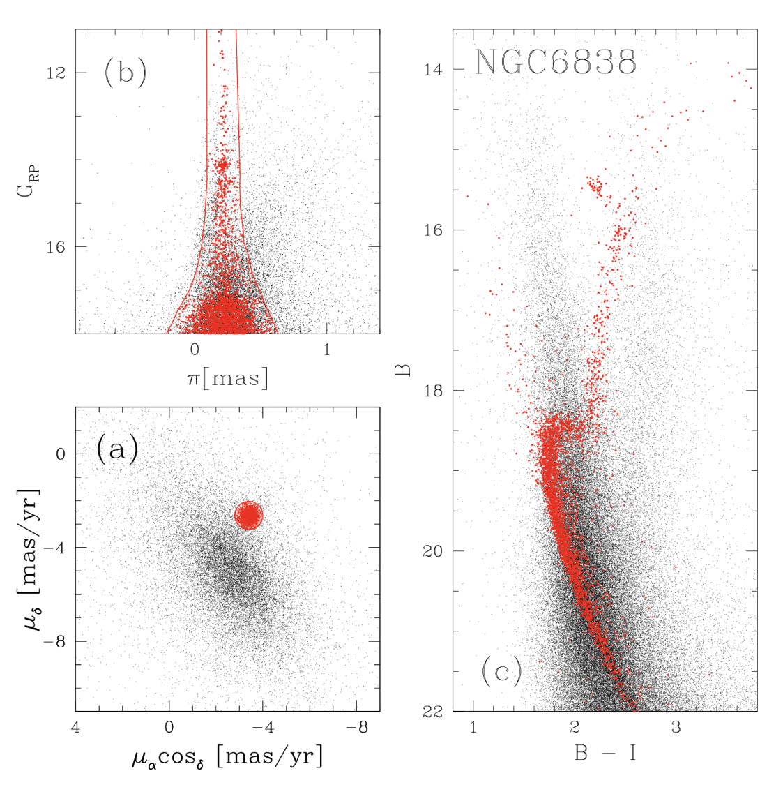
Figure 1: This figure illustrates the procedure to select probable members of NGC 6838. Panel (a) shows the VPD of proper motions for stars in the cluster field. Panel (b) show $G_{\rm RP}$ as a function of the parallax $\pi$ and the two lines drawn by eye that encloses probable cluster members. The B vs. B-I CMD is illustrated in panel (c). Cluster members selected are represented with red symbols.

1 Introduction

It is now well established that most globular clusters (GCs) host two main groups of stars: a first stellar population (hereafter 1G) with chemical composition that resembles halo field stars, and a second population (2G) of stars enriched in helium, nitrogen and sodium and depleted in carbon and oxygen (see Bastian et al., 2018; Gratton et al., 2019; Milone & Marino, 2022, for recent reviews). Multiple populations have been widely investigated during the past decades but their origin still represents one of the most intriguing open issues in stellar astrophysics. According to some scenarios, the multiple populations are the signature of multiple star-formation episodes, where 2G stars originate from material polluted by more-massive 1G stars (e.g. D’Antona et al., 2016; Decressin et al., 2007; de Mink et al., 2009; Denissenkov & Hartwick, 2014; Jang et al., 2014; Jang & Lee, 2015; Lee et al., 1999; Lee & Jang, 2016; Renzini et al., 2022). Other formation scenarios suggest that all GC stars are coeval and that accretion of polluted material onto pre-MS stars is responsible for the chemical composition of 2G stars (e.g. Bastian et al., 2013; Gieles et al., 2018). As an alternative, stellar mergers are responsible for multiple populations in GCs (Wang et al., 2020).

Photometry, together with spectroscopy, is the main technique to identify and characterize multiple populations in GCs, and various photometric diagrams have been exploited in the past decade to disentangle 1G and 2G stars. Numerous studies, based on colour-magnitude diagrams (CMDs), two-colour diagrams, and pseudo CMDs that are derived from suitable combinations of stellar magnitudes filters of Hubble space telescope (HST), have provided an homogeneous and extensive analysis of the multiple-population phenomenon in Galactic and extragalactic GCs (e.g. Milone et al., 2012b, 2020a; Piotto et al., 2015; Niederhofer et al., 2017; Lagioia et al., 2019; Jang et al., 2021).

The pseudo two-colour diagram dubbed ’chromosome map’ (ChM) resulted to be one of the most efficient diagnostic tools to identify and characterize multiple populations. The traditional ChM, which is built with a suitable combination of stellar magnitudes in the F275W, F336W (or F343N), F438W, and F814W filters, is very sensitive to the chemical composition of GC stars (mostly on the content on helium, nitrogen, carbon, and oxygen). It has allowed us to identify and characterize multiple population phenomenon within about sixty Galactic GCs, with unprecedented detail (Milone et al., 2015, 2017a).

More recently, various authors introduced additional ChMs based on HST photometry. Some ChMs are composed of F336W (or F343N), F438W, and F814W magnitudes alone, thus avoiding the most time-demanding F275W filter (Zennaro et al., 2019; Larsen et al., 2019; Milone et al., 2020a). In addition, ChMs build with the F275W, F280N, F343N, and F373N filters allowed us to disentangle stellar populations with different Mg abundances along the RGB (Milone et al., 2020b), whereas ChMs composed of appropriate combinations of optical and near-infrared filters (e.g. F606W, F814W, F110W, and F160W) are sensitive to multiple populations with different oxygen abundances among very-low mass stars (Milone et al., 2017b; Milone & Marino, 2022).

One of the major limitations is the small field of view of HST cameras, which restricts most of the studies on Galactic GCs to the innermost cluster regions. Clearly, wide-field photometry is mandatory to extend the investigation of multiple populations to the entire cluster.

To overcome the main limitation of HST, ground-based facilities are used to investigate the multiple stellar populations in Galactic GCs by means of photometric diagrams that are sensitive to the chemical composition of the distinct populations. The most-used diagrams involve CMDs and pseudo-CMDs built with Ströemgren photometry (e.g. Grundahl et al., 1998; Yong & Grundahl, 2008), photometry from appropriate narrow-band filters (Lee, 2017), or appropriate combinations of the $U$, $B$, $V$ and $I$ Johnson-Cousin bands (Marino et al., 2008; Milone et al., 2010, 2012a; Dondoglio et al., 2021).

In this context, photometric diagrams made with the $C_{\rm U,B,I}=(U-B)-(B-I)$ pseudo colour, are efficient tools to disentangle stellar populations with different light-element abundances along the red-giant branch (RGB), whereas CMDs made with $B-I$ colour are sensitive to stellar populations with different helium abundances (e.g. Monelli et al., 2013; Cordoni et al., 2020). Although these diagrams are widely used to identify multiple populations in GCs, they are less efficient than ChMs to disentangle the distinct stellar populations of several GCs.

Hartmann et al. (2022) first derived a ChM from ground-based photometry, by using the $U$ band together with the narrow-band filters centered around 3780Å  and 3950Å. In this paper, we introduce a new ChM, which is based on photometry in the $U$, $B$, and $I$ bands, and provides improved identification of multiple populations from ground-based Johnson-Cousin photometry. In addition to the filter choice, the correction of the effect of differential reddening on stellar magnitudes is a crucial ingredient to disentangle multiple populations in photometric diagrams (Milone et al., 2012a). Hence, we derive and publicly release high-resolution reddening maps.

The paper is organized as follows. Data and data analysis are described in Section 2, where we also investigate the differential reddening and illustrate the reddening maps. The method to derive the ChM is described in Section 3, where we also provide some applications on how to characterize multiple populations in NGC 288 by using the ChM. The ChMs of RGB stars in 29 Galactic GCs are presented in Section 4, while Section 5 is dedicated to the ChM along the asymptotic-giant branch (AGB). Summary and conclusions follow in Section 6.

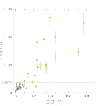
Figure 2: $\sigma_{\Delta E(B-V)}$ against the average reddening from of the host cluster (from the 2010 version of the Harris, 1996, catalog). $\sigma_{\Delta E(B-V)}$ indicates 1$\sigma$ value of average reddening of each of 100 $\times$ 100 arcsec cells dividing the field of view of a GC. Photometry of 18 GCs with $\sigma_{\Delta E(B-V)}$>0.0075 coloured in yellow have been corrected for the effect of differential reddening in this work.

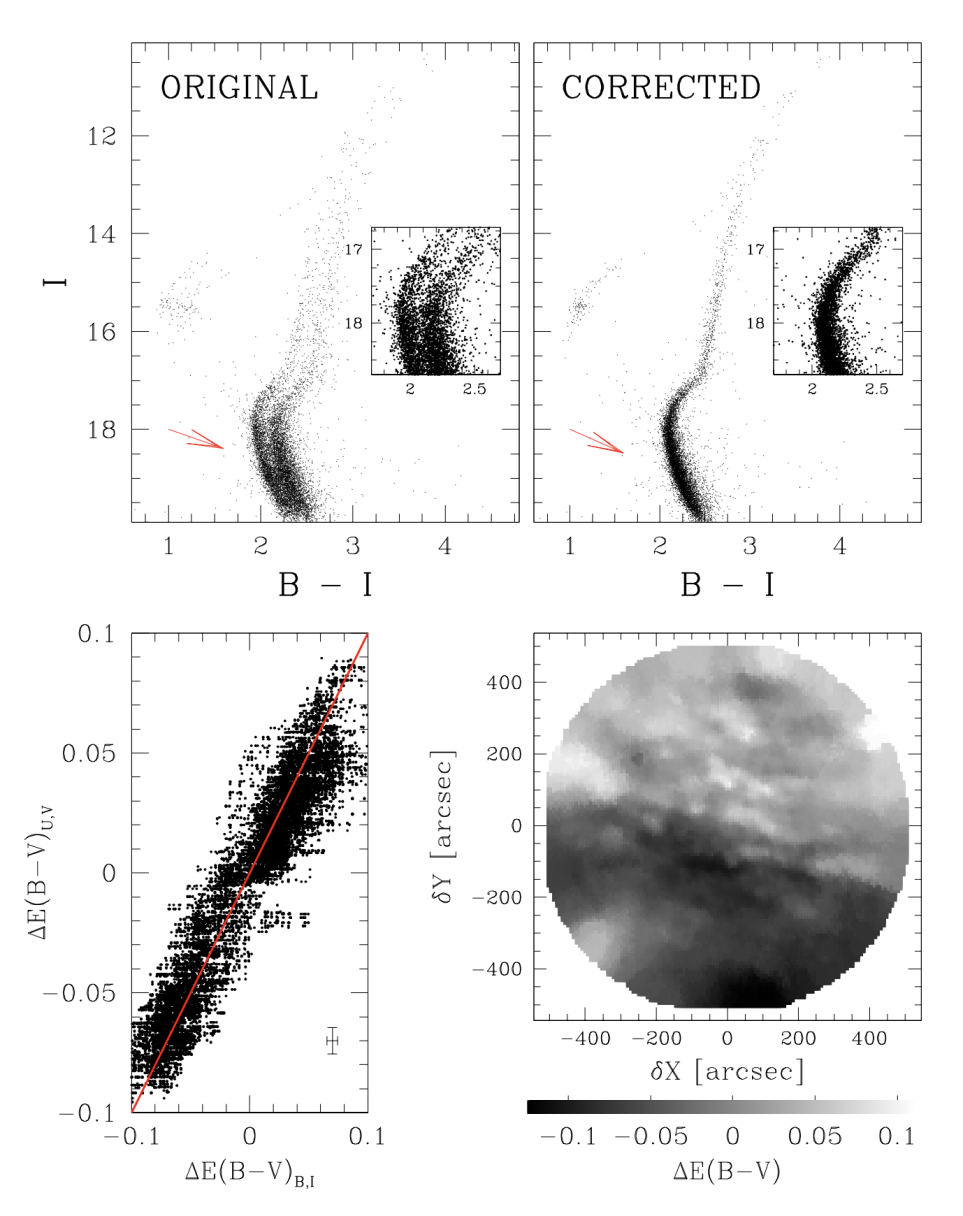
Figure 3: Upper panels: comparison of the original $I$ versus $B-I$ CMD of NGC 4372 (left) and the CMD corrected for differential reddening (right). A zoom of each CMD around the SGB is plotted in the insets. The reddening vectors are indicated with red arrows. Lower panels: differential reddening map (right). The levels of grey correspond to different $\Delta$E($B-V$) values as indicated by the scale on the bottom. The left panel compares the differential reddening values inferred from the $I$ versus $B-I$ and the V versus $U-V$ CMD. The red line indicates the perfect agreement.

2 Data and Data Analysis

To derive differential-reddening maps in the field of view of 43 GCs we use the photometry in the $U$, $B$, $V$, $I$ photometric bands from Stetson et al. (2019) and coordinates, proper motions, and parallaxes from the Gaia early Data Release 3 (Gaia Collaboration et al., 2021, eDR3). Photometry has been derived by Peter Stetson from images collected with various ground-based telescopes and by using the methods and the computer programs by Stetson (2005) and has been calibrated on the reference system by Landolt (1992). Details on the data and the data analysis are provided by Stetson et al. (2019) .

2.1 Selection of cluster members

To unambiguously identify multiple populations from the photometry, we need to select a sample of well-measured stars and separate field stars from cluster members. To do this, we combined the ground-based stellar photometry with proper motions and parallaxes from Gaia Collaboration et al. (2021).We selected the bulk of cluster members by following the procedure by Cordoni et al. (2018), which is illustrated in Figure 1 for NGC 6838.

In a nutshell, we first selected stars with cluster-like kinematics, based on their position in the vector-point diagram (VPD) of proper motions. As an example, the probable members of NGC 6838 are clusters around ($\mu_{\rm\alpha}$cos$\delta$, $\mu_{\rm\delta}$) $\sim$ ($-$3.4,$-$2.6) in the VPD of Figure 1a. Hence, we draw by hand the red circle to separate bona-fides cluster members from field stars. In addition, we select stars with cluster-like parallaxes, $\pi$, based on their position in the $G_{\rm RP}$ vs. $\pi$ plane. As shown in Figure 1b, the two red lines that we draw by eye enclose the majority of NGC 6838 stars. The selected well-measured cluster members are represented with red symbols in the $B$ versus $B-I$ CMD of Figure 1c. We will use these stars to derive high-resolution reddening maps and to investigate multiple stellar populations.

2.2 Differential Reddening

The distribution of foreground interstellar gas and dust in the directions of the studied GCs is rarely uniform. As a consequence, the amount of reddening suffered by each cluster can vary from one star to another.

To quantify the amount of reddening variation across the field of view of each cluster and to correct the photometry for the effect of differential reddening, we adapted the method by Milone et al. (2012a) to the photometric catalogs by Stetson et al. (2019). We used the $I$ vs. $B-I$ and $V$ vs. $U-V$ CMDs to derive two distinct determinations of the amount of differential reddening suffered by each star in each cluster ($\Delta$E($B-V$)_B,I, and $\Delta$E($B-V$)_U,V, respectively). The values of $\Delta$E($B-V$)_B,I and $\Delta$E($B-V$)_U,V are then averaged together to derive improved values of differential-reddening.

We first selected a sample of reference stars, including bright-MS, sub-giant branch (SGB), and RGB cluster members, and calculated the corresponding fiducial line in the CMD. Then, we used the absorption coefficients by Schlegel et al. (1998) to determine the direction of the reddening and measure the colour and magnitude distance of each reference star from the fiducial along the reddening direction, $d$. The values of $d$ have been used for two main purposes: i) deriving low-resolution reddening maps, which allow to homogeneously compare the variation of reddening in the direction of each cluster, and ii) correct the photometry for the effect of differential reddening.

To quantify the amount of differential reddening in the direction of each cluster, we divided the field of view into 100$\times$100 arcsec cells. We estimated the amount of differential reddening of each cell by calculating the median value of $d$ for the reference stars in the cell. This quantity is converted into a differential reddening value by using the coefficients by Schlegel et al. (1998). We provide in Table 3 the 68.27^th percentile of the differential-reddening values, $\sigma_{\Delta E(B-V)}$, the difference between the 98^th and the second percentile of the differential-reddening distributions $\Delta$E(B$-$V)_98%-2%, and the maximum radial distance used to derive differential reddening, R_max. The uncertainties associated with these values are calculated with a bootstrap analysis based on 1,000 samples created by a random sampling with replacement of the values of differential reddening. For each extraction we derived the values of $\sigma_{\Delta E(B-V)}$ and $\Delta$E(B$-$V)_98%-2% by using the procedure described above. We considered as our best uncertainties estimates, the value of the random mean scatter of the 1,000 determinations of $\sigma_{\Delta E(B-V)}$ and $\Delta$E(B$-$V)_98%-2%.

The values of $\sigma_{\Delta E(B-V)}$ range from less than 0.005 mag to more than 0.050 mag, whereas $\Delta$E(B$-$V)_98%-2% varies from less than 0.01 mag to $\sim$0.19 mag. As shown in Figure 2, $\sigma_{\Delta E(B-V)}$ correlates with the average reddening of the host cluster (from the 2010 version of the Harris, 1996, catalog).

The main effect of differential reddening on the photometry is a colour and magnitude broadening of the various sequences of the CMD. To correct photometry for this effect, in 18 GCs with $\sigma_{\Delta E(B-V)}$>0.0075 mag (yellow dots in Figure 2), we derived the amount of differential reddening associated with all stars in the catalog. For each star, we selected the sample of $35-75$ neighboring reference stars and calculated the median distance along the reddening line. We imposed that the maximum radius of the region that includes the reference stars is smaller than 2 arcmin. Hence, the value of R_max, is fixed on the basis of this criterion. The only exception is Palomar 11 where, due to the small number of stars, we used a threshold of 2.5 arcmin. We excluded each reference star from the determination of its own differential reddening. The uncertainty associated with differential-reddening determination is estimated as the random mean scatter of the distance values divided by the square root of $N-1$. See Milone et al. (2012a) for details.

Some results from this procedure are illustrated in Figure 3 for NGC 4372. Upper panels of Figure 3 compare the original $I$ versus $B-I$ CMD of NGC 4372 (left) with the CMD corrected for differential reddening (right). The inset of each panel shows a zoom in the SGB region, where the effect of the correction is more evident.

Lower-right panel of Figure 3 shows the resulting differential reddening map, which reveals spatial variations of $\sim 0.19$ mag in $\Delta E(B$-$V)$, over the field of view. The lower-left panel of Figure 3 compares $\Delta E(B-V)_{\rm B,I}$ and $\Delta E(B-V)_{\rm U,V}$. The average difference between the two differential-reddening determinations is nearly zero (0.0009 mag), but the random median scatter of 0.016 mag, is larger than the typical uncertainty associated with our reddening determinations. Indeed, in addition to differential reddening, small inaccuracies of the PSF model and of the sky determination can contribute to the broadening of the sequences in the CMD. Their presence is indicated by the fact that differences between $\Delta E(B-V)_{\rm B,I}$ and $\Delta E(B-V)_{\rm U,V}$ are typically larger than the observational errors (see Anderson et al., 2008; Milone et al., 2012a, for discussion). The values of the 68.27^th percentile of differential-reddening difference $\Delta E(B-V)_{\rm B-I}$ - $\Delta E(B-V)_{\rm U-V}$ are provided in Table 3.

The differential-reddening maps for the eighteen GCs with $\sigma_{\Delta E(B-V)}$>0.0075 mag are illustrated in Figure 4 and Figure 5 .

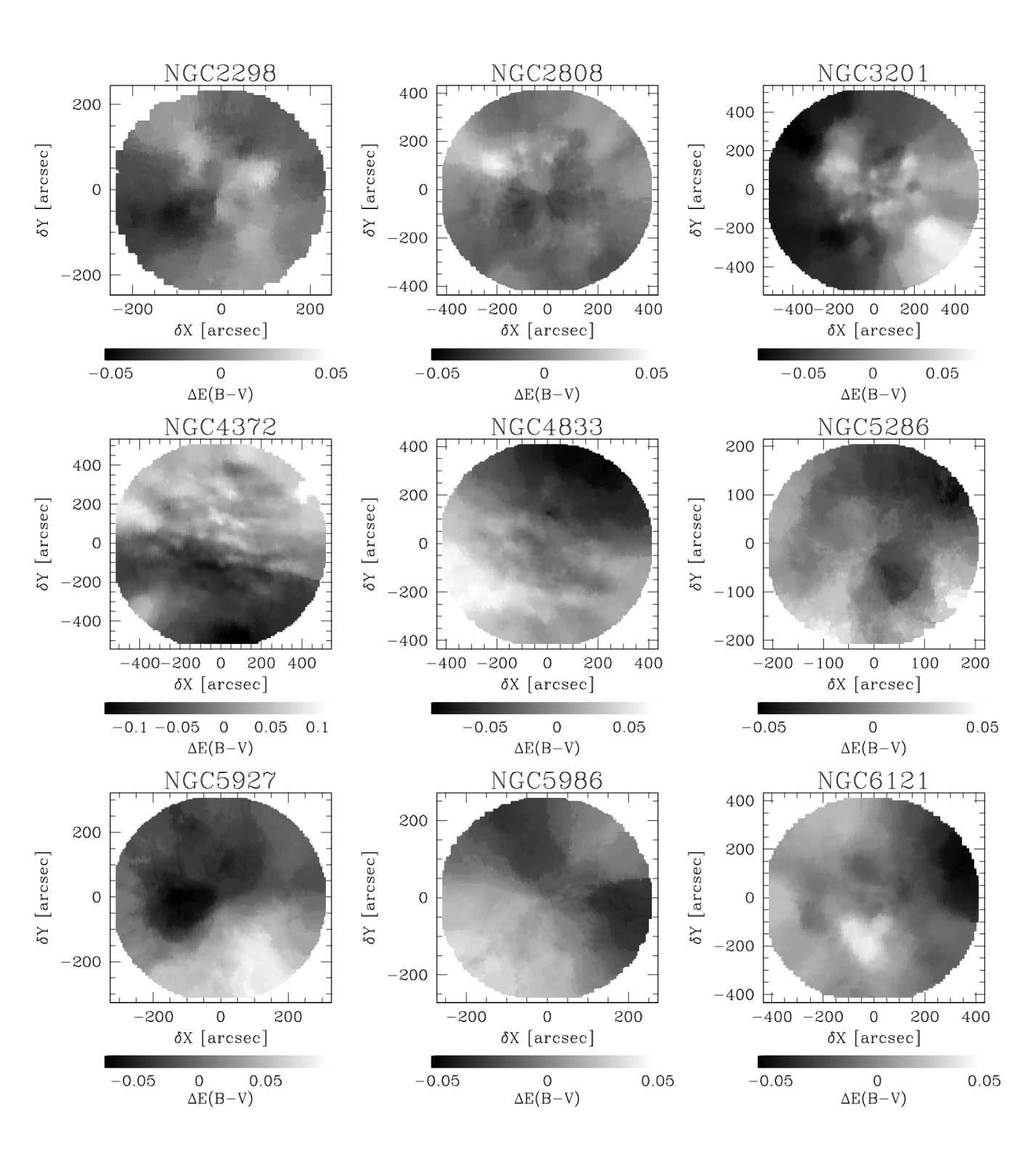
Figure 4: Differential-reddening maps of the regions in front of NGC 2298, NGC 2808, NGC 3201, NGC 4372, NGC 4833, NGC 5286, NGC 5927, NGC 5986, and NGC 6121.

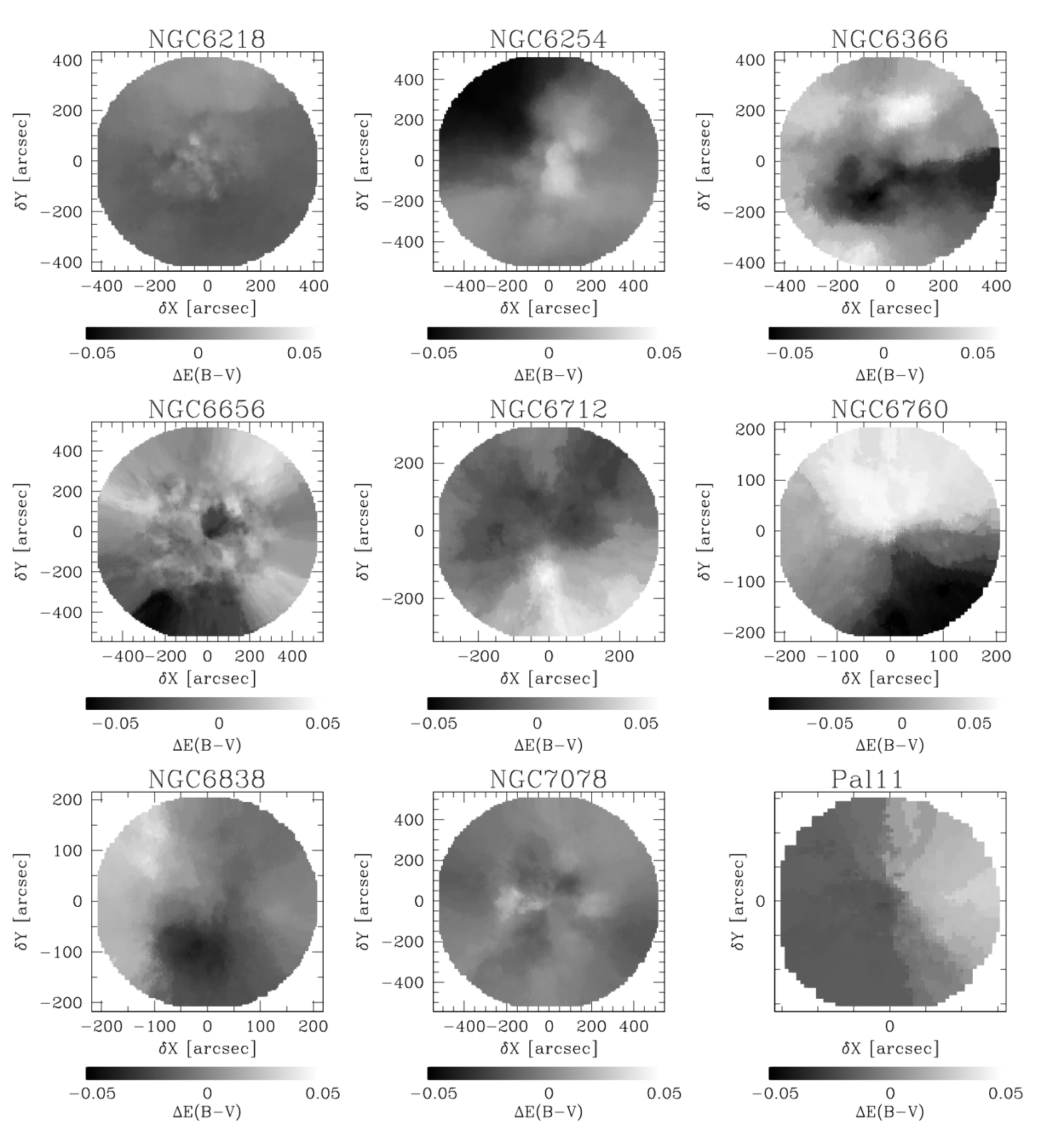
Figure 5: Same as Figure 4 but for NGC 6218, NGC 6254, NGC 6366, NGC 6656, NGC 6712, NGC 6760, NGC 6838, NGC 7078, and Palomar 11.

Figure 6: Comparison of the original $I$ versus $B-I$ CMDs of NGC 3201, NGC 4833, NGC 5927, and NGC 6366 (left panels) with the CMDs corrected for differential reddening (midle panels). The right panels show the $U$ vs. $U-I$ CMD of the Type II GCs NGC 1851, NGC 1261, NGC 6934 and NGC 7089. Red-RGB stars are coloured aqua.

As an example, Figure 6 compares the original CMDs of selected cluster members of NGC 3201, NGC 4833, NGC 5927, and NGC 6366 with the corresponding CMDs corrected for differential reddening. We also show the $U$ vs. $U-I$ CMDs of selected cluster members in the Type II GCs NGC 1851, NGC 1261, NGC 6934 and NGC 7089. The blue and red-RGBs are clearly visible and we used aqua colours to highlight red-RGB stars.

3 Chromosome maps of RGB stars

To derive the ChM of RGB stars from wide-field ground-based photometry, we combined the $I$ vs. $B-I$ CMD and the $I$ vs. $C_{\rm U,B,I}$ pseudo CMD of each GC. The procedure is illustrated in Figure 7 for NGC 288, which is used as a test case and is based on the method by Milone et al. (2015, 2017a).

The ChM is derived from the $I$ vs. $C_{\rm U,B,I}$ pseudo CMD and the $I$ vs. $B-I$ CMD plotted in panels (a1) and (b1), respectively. The red and blue fiducial lines superimposed on each diagram are derived by hand and mark the red and blue boundary of the RGB, respectively.

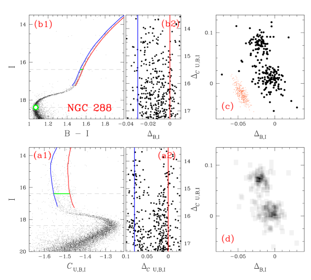
Figure 7: This figure illustrates the procedure to derive the $\Delta c_{\rm U,B,I}$ versus $\Delta_{\rm B,I}$ Chromosome map for the prototypical cluster NGC 288. Panels (a1) and (b1) show the $I$ versus $C_{\rm U,B,I}$ pseudo-CMD and $I$ versus $B-I$ CMD of NGC 288. The green circle in panel (b1) marks the MS turnoff, whereas the two horizontal dotted lines in panels (a1) and (b1) are placed at the magnitude level of the MS turnoff and 2.0 $I$ mag above it. The blue and red lines mark the boundaries of the RGB, while the green segments in the panels (a1) and (b1) indicate the $B-I$ colour and the $C_{\rm U,B,I}$ pseudo-colour separation between the two lines at 2.0 $I$ mag above the MS turnoff. The ‘verticalized’ $I$ versus $\Delta c_{\rm U,B,I}$ and $I$ versus $\Delta_{\rm B,I}$ diagrams for RGB stars are plotted in panels (a2) and (b2), respectively, where the red and blue vertical lines correspond to the RGB boundaries in panels (a1) and (b1) that translate into vertical lines in panel (a2) and (b2). The RGB stars used to construct the chromosome map in panel (c) are represented in panels (a2) and (b2), where $\Delta c_{\rm U,B,I}$ and $\Delta_{\rm B,I}$ are plotted against $I$. Panel (d) shows the Hess diagram for stars in panel (c).

The RGB boundaries are used to ‘verticalize’ the two diagrams in a way that each of them translates into a vertical line. Specifically, we defined

$$\Delta_{\rm B,I}=W_{\rm B,I}\frac{X-X_{\rm fiducialR}}{X_{\rm fiducialR}-X_{\rm fiducialB}}$$ (1)

$$\Delta c_{\rm U,B,I}=W_{C\rm U,B,I}\frac{Y-Y_{\rm fiducialB}}{Y_{\rm fiducialR}-Y_{\rm fiducialB}}$$ (2)

where $X=B-I$ and $Y=C_{\rm U,B,I}$ and ‘fiducial R’ and ‘fiducial B’ correspond to the red and the blue fiducial lines, respectively. The quantities $W_{\rm B,I}$ and $W_{C\rm U,B,I}$ are indicative of the RGB widths. Their values correspond the colour separation between the RGB boundaries 2.0 $I$ mag above the main-sequence (MS) turnoff.

The ‘verticalized’ $I$ versus $\Delta c_{\rm U,B,I}$ and $I$ versus $\Delta_{\rm B,I}$ diagrams for RGB stars are plotted in panels (a2) and (b2) of Figure 7, respectively, where the red and blue vertical lines correspond to the RGB boundaries in panels (a1) and (b1). The $\Delta_{\rm B-I}$ and $\Delta c_{\rm U,B,I}$ pseudo colours are used to derive the ChM plotted in panel (c), where we only included RGB stars with $13.0<I<17.5$ mag. As highlighted by the Hess diagram shown in panel (d), the ChM of NGC 288 reveals two distinct stellar populations clustered around ($\Delta_{\rm B,I}$,$\Delta c_{\rm U,B,I}$),=(0.0,0.0) mag and ($-$0.02,0.07) mag.

For completeness, we show in Figure 8 the $\Delta_{\rm U,B}$ vs. $\Delta_{\rm B,I}$ ChM of RGB stars in NGC 288. This ChM is similar to the ChM introduced in Figure 7, but is derived from the $I$ vs. $U-B$ and $I$ vs. $B-I$ CMDs. Here, one group of stars is clustered around the origin of the reference frame, whereas the remaining stars are distributed around ($\Delta_{\rm B,I}$,$\Delta_{\rm U,B}$)$\sim$($-$0.2,0.06) mag. Although for simplicity, this paper is focused on the $\Delta_{\rm B-I}$ vs. $\Delta c_{\rm U,B,I}$ diagrams alone, the ChM introduced in Figure 8 provides an additional tool to investigate multiple populations in GCs.

Next Section 3.1 takes advantage of isochrones and synthetic spectra for better understanding the position of stars in the ground-based ChM. In Section 3.2 we compare the ChMs of NGC 288 from HST and ground-based photometry, while in Sections 3.3 and 3.4 we illustrate some applications of the ChM of NGC 288 to constrain the chemical composition of 1G and 2G stars, and investigate their radial distributions.

3.1 Theoretical interpretation

To investigate the position of stars with different contents of He, C, N, O, and Fe in the ChM of Type I GCs, we started deriving the colours and magnitudes of the Dartmouth isochrones (Dotter et al., 2008) with the same age of 13 Gyr, metallicity, [Fe/H]=$-$1.5, and [$\alpha$/Fe]=0.4, but different chemical compositions. To do this, we followed the procedure by Milone et al. (2018), which uses model atmospheres and synthetic spectra. We identified fifteen points along the isochrone, I1, that is representative of 1G stars and extracted their stellar parameters. We calculated two spectra for each combination of effective temperature and gravity, including a reference spectrum that resembles 1G stars and several comparison spectra that share the same chemical composition as 2G stars. We assumed for 1G stars Y=0.246, solar-scaled abundances of carbon and nitrogen, and [O/Fe]=0.4, while the chemical compositions used for 2G stars are listed in Table 1.

We used the ATLAS12 and SYNTHE programs (Kurucz, 1970; Kurucz & Avrett, 1981; Kurucz, 2005; Sbordone et al., 2004, 2007) to derive model atmosphere structures and compute synthetic spectra. When we modified the helium content we accounted for the variation in effective temperature and gravity predicted by the isochrones by Dotter et al. (2008). We integrated each spectrum over the bandpasses of the $U,B,I$ filters to calculate synthetic magnitudes and derive the magnitude differences, namely $\delta U$, $\delta B$, and $\delta I$, between the comparison and the reference spectrum. Isochrones 2–4 are derived by adding to the isochrone I1 the corresponding values of $\delta U$, $\delta B$, and $\delta I$.

In addition, we used two isochrones from Dotter et al. (2008) that differ from I1 because a variation in helium alone (I5) or in iron abundance alone (I6). These isochrones would mimic the subpopulations of 1G stars with different chemical composition (e.g.  Milone et al., 2015; Milone & Marino, 2022; Marino et al., 2019a; Legnardi et al., 2022).

Table 1: Chemical composition of the six isochrones shown in Figure 9. All isochrones have ages of 13 Gyr and [$\alpha$/Fe]=0.4.

Isochrone	Y	[C/Fe]	[N/Fe]	[O/Fe]	[Fe/H]
I1	0.246	0.00	0.00	0.40	$-$1.50
I2	0.256	$-$0.05	0.53	0.35	$-$1.50
I3	0.276	$-$0.10	0.93	0.20	$-$1.50
I4	0.306	$-$0.50	1.21	$-$0.10	$-$1.50
I5	0.266	0.00	0.00	0.40	$-$1.50
I6	0.246	0.00	0.00	0.40	$-$1.45

The isochrones I1–I6 are plotted in the $M_{\rm I}$ vs. $M_{\rm B}-M_{\rm I}$ CMD and the $M_{\rm I}$ vs. $C_{\rm U,B,I}$ pseudo CMD of Figure 9 (left and middle panel, respectively), where we also show the corresponding $\Delta_{C\rm U,B,I}$ vs. $\Delta_{\rm B,I}$ ChM for RGB stars. Clearly, the new ChM would allow us to separate 1G stars, which distribute around the origin of the reference frame, from 2G stars.

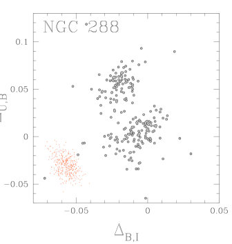
Figure 8: $\Delta_{\rm U,B}$ versus $\Delta_{\rm B,I}$ ChM for RGB stars of NGC 288.

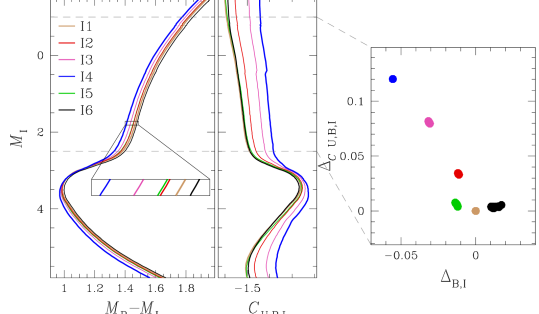
Figure 9: The six coloured lines plotted in the left and middle panel represent the isochrones I1–I6 (see Table 1 for details on their chemical compositions). The $\Delta_{C\rm U,B,I}$ vs. $\Delta_{\rm B,I}$ ChM of the RGB stars between the dashed horizontal lines is plotted in the right panel.

Our analysis of synthetic spectra reveals that the $I$ vs. $B-I$ CMD is mainly affected by helium variations between 1G and 2G RGB stars. The $I$ vs. $C_{\rm U,B,I}$ diagram of monometallic GCs is mostly sensitive to nitrogen variation among the different stellar populations. The ChM of Figure 9 combines these two diagrams, thus providing more information on the chemical composition of multiple populations than each individual diagram.

Moreover, since the distinct stellar populations of most GCs have different values of $\Delta_{C\rm U,B,I}$ and $\Delta_{\rm B,I}$, the ChM would provide a wider separation between 1G and 2G stars of most GCs rather then the $I$ vs. $B-I$ and the $I$ vs. $C_{\rm U,B,I}$ diagrams, separately. In particular, it would allow us to detect extended or multimodal sequences of 1G stars.

An additional advantage of the ChM is that the RGB stars of each simple stellar population would be distributed in a nearly point-like ares of the ChM. Hence, the distribution of stars in the ChM is poorly dependent on the evolutionary phase along the RGB.

3.2 Comparison with the traditional ChM from HST

To further investigate the distribution of 1G and 2G stars along the ground-based ChM, we investigate the ChM stars for which both ground-based and HST photometry are available. It is widely accepted that 1G stars are clustered around the origin of the traditional ChM derived from HST photometry, while 2G stars are distributed towards larger and smaller values of $\Delta c_{\rm F275W,F336W,F814W}$ and $\Delta_{F275W,F814W}$, respectively (Milone et al., 2015).

As an example, probable 1G and 2G stars of NGC 288 are coloured red and blue, respectively, in the upper-left panel of Figure 10 where we show the $\Delta c_{\rm F275W,F336W,F814W}$ versus $\Delta_{F275W,F814W}$ from Milone et al. (2017a). The upper-right panel of Figure 10 shows the $\Delta c_{\rm U,B,I}$ ChM of NGC 288 derived in this paper (right). The probable 1G and 2G stars identified in the upper-left panel and for which both ground-based and HST photometry is available are marked with large squares.

Results from this comparison confirm the predictions from the simulated ChM of Section 3.1. Indeed, the two groups of selected 1G and 2G stars populate the regions of the upper-right panel ChM with small and large values of $\Delta c_{\rm U,B,I}$ and $\Delta_{\rm B,I}$, respectively. Two stars that are classified as 2G in the HST ChM but exhibit low values of $\Delta c_{\rm U,B,I}$ together with one 1G star with large $\Delta c_{\rm U,B,I}$ values are possible exceptions.

3.3 Chemical tagging of stellar populations along the ChM of NGC 288

In the past decades, the synergy of spectroscopy and photometry from both HST and ground-based facilities has provided major advances towards the understanding of the multi-population phenomenon. Early results based on wide-band ground-based photometry revealed that Na-poor/O-rich and Na-rich/O-poor stars define different RGB sequences in the $B$ vs. $U-B$ CMDs of M 4 and NGC 6752 (Marino et al., 2008; Milone et al., 2010). Moreover, 1G and 2G stars of 47 Tucanae populate distinct sequences in the $B$ vs. $U-B+I$ diagram (Milone et al., 2012b) and in the $V$ vs. $C_{\rm U,B,I}$ diagram (Monelli et al., 2013). In general, the sodium and oxygen abundances correlate and anticorrelate, respectively, with the $C_{\rm U,B,I}$ value, as shown by Monelli et al. (2013) for 15 GCs. Similar conclusion that the colour of RGB stars depends on light-element abundance is provided by pioneering works based on Ströemgren photometry (Grundahl et al., 1998; Yong & Grundahl, 2008; Carretta et al., 2011).

Similarly, a lot of efforts have been dedicated to chemically characterize the stellar populations along the ChMs derived from both HST (e.g. Milone et al., 2015; Carretta et al., 2018; Marino et al., 2019a), and ground-based photometry (Hartmann et al., 2022).

In the bottom-left panel of Figure 10 we use the $\Delta c_{\rm U,B,I}$ and $\Delta_{\rm B,I}$ ChM to identify by eye the probable 1G and 2G stars of NGC 288 (red and blue circles, respectively), based on their position on the ground-based ChM alone.

To constrain their chemical composition, we use the chemical abundances inferred by Carretta et al. (2009) from high-resolution spectroscopy. Some results are illustrated in the bottom-right panel of Figure 10, where we plot [Na/Fe] vs. [O/Fe]. Stars for which both photometry and spectroscopy is available are plotted with large dots. Clearly, 1G stars are Na-poor and O-rich, whereas 2G stars are sodium enhanced and oxygen depleted. The average abundances for the 1G stars and the 2G stars are listed in Table 2 and are in agreement with the results from Marino et al. (2019a), where 1G and 2G stars have been identified on the traditional ChM from (HST). However, the average abundances inferred in this paper have smaller errors than those provided by Marino and collaborators, thanks to the large number of spectroscopic targets for which ground-based photometry is available.

Table 2: Average abundances of oxygen, sodium, and iron of 1G and 2G stars in NGC 288 inferred in this paper and by Marino et al. (2019a).

	[O/Fe]	[Na/Fe]	[Fe/H]
		This paper
1G	0.34$\pm$0.04	0.05$\pm$0.02	$-$1.21 $\pm$ 0.01
2G	0.06$\pm$0.08	0.47$\pm$0.03	$-$1.22 $\pm$ 0.01
		Marino et al. (2019a)
1G	0.25$\pm$0.09	0.10$\pm$0.04	$-$1.21$\pm$0.01
2G	0.11$\pm$0.13	0.51$\pm$0.04	$-$1.23$\pm$0.02

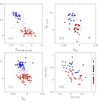
Figure 10: Upper panels. $\Delta c_{\rm F275W,F336W,F814W}$ versus $\Delta_{F275W,F814W}$ ChM of NGC 288 from HST photometry (Milone et al., 2017a). The probable 1G and 2G stars selected by Milone and collaborators are coloured red and blue, respectively (upper-left). Reproduction of the $\Delta c_{\rm U,B,I}$ and $\Delta_{\rm B,I}$ ChM derived in Figure 7. Large squares represent stars with both HST and ground-based photometry (upper-right). Bottom panels. The 1G and 2G stars identified in the $\Delta c_{\rm U,B,I}$ and $\Delta_{\rm B,I}$ plane are represented with red and blue circles, respectively, in the bottom-left ChM. Sodium versus oxygen abundances for RGB stars of NGC 288 (Carretta et al., 2009). Stars for which [O/Fe] estimates are not available are plotted on the right side of the vertical line in the panel. Stars included in the ChM for which sodium abundances are available are represented with large dots.

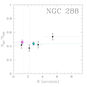
Figure 11: Fraction of 2G stars of NGC 288 against the radial distance from the cluster center. Black dots are derived in this paper, whereas the magenta starred symbol indicates the fraction of 2G stars measured by Milone et al. (2017a) from HST photometry. The cyan dot marks the average fraction of 2G stars from ground-based photometry. The horizontal segments mark the radial interval corresponding to each point. Vertical dotted and dashed-dotted lines indicate the core and half-light radius (from the 2010 version of the Harris, 1996, catalog).

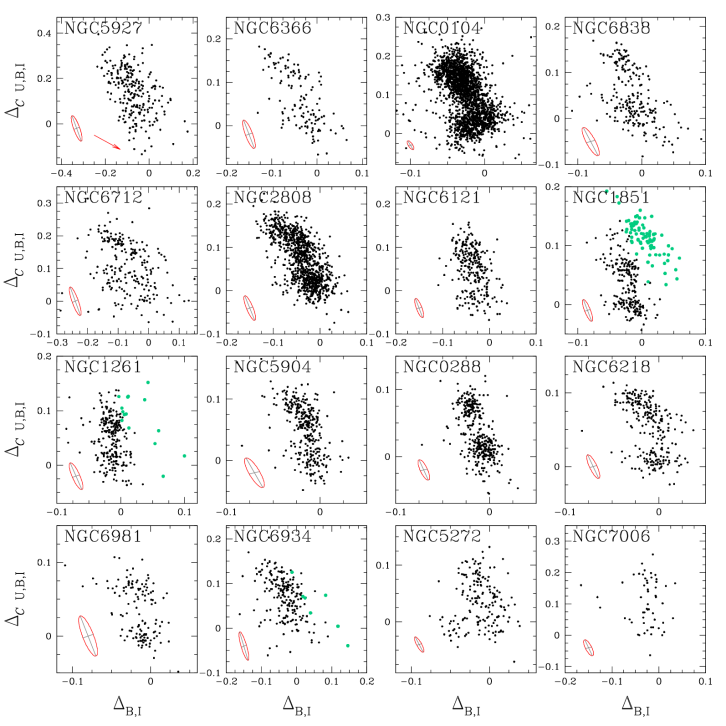
Figure 12: $\Delta c_{\rm U,B,I}$ versus $\Delta_{\rm B,I}$ diagrams (or chromosome maps) for RGB stars in the GCs NGC 5927, NGC 6366, NGC 104, NGC 6838, NGC 6712, NGC 2808, NGC 6121, NGC 1851, NGC 1261, NGC 5904, NGC 288, NGC 6218, NGC 6981, NGC 6934, NGC 5272, and NGC 7006. The clusters are sorted according by metallicity, from the most metal-rich to the most metal-poor. Aqua symbols mark red-RGB stars of Type II GCs. The arrow n the top-right panel indicates the reddening vector and correspond to a reddening variation $\Delta$E($B-V$) = 0.05 mag

.

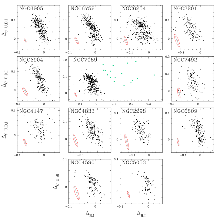
Figure 13: As in Figure 12, but for NGC 6205, NGC 6752, NGC 6252, NGC 3201, NGC 1904, NGC 7089, NGC 7492, NGC 4147, NGC 4833, NGC 2298, NGC 6809, NGC 4590, and NGC 5053.

3.4 The radial distribution of multiple populations in NGC 288

Most scenarios for the formation of multiple populations predict that 2G stars form in the cluster center (e.g. D’Ercole et al., 2008; Denissenkov & Hartwick, 2014; D’Antona et al., 2016; Gieles et al., 2018; Renzini et al., 2015, and references therein). Due to dynamic evolution, some GCs can retain some memory of the initial distribution of 1G and 2G stars, while the multiple populations of other clusters can fully mixed (e.g. Vesperini et al., 2013; Dalessandro et al., 2019). Hence, the present-day spatial distribution of multiple populations in GCs would provide valuable tests for the formation scenarios. Work based on both spectroscopy and photometry show that 2G stars of various GCs (e.g. 47 Tucanae, NGC 2808, M 3, NGC 5927 among the others) (e.g. Cordero et al., 2014; Milone et al., 2012a; Vanderbeke et al., 2015; Lee, 2017; Dondoglio et al., 2021) are more centrally concentrated than the 1G, whereas multiple populations of other clusters (e.g. NGC 6752, NGC 6362, M 5, NGC 6366, NGC 6838) share the same radial distribution (e.g. Vanderbeke et al., 2015; Lee, 2017; Milone et al., 2019; Dalessandro et al., 2018; Cordoni et al., 2020; Dondoglio et al., 2021). Some authors suggest that a few clusters can exhibit reverse radial distribution in contrast with theoretic predictions (see Hartmann et al., 2022, for the case of NGC 3201).

To derive the population ratios in NGC 288 we used the method by Milone et al. (2017a, see their Figure 8). We first rotated the ChM in a reference frame, $\Delta_{2}$ vs. $\Delta_{1}$, where the abscissa follows the direction of 1G stars. Then, we derived the histogram distribution of the ordinate $\Delta_{2}$ and fitted the histogram of candidate 1G stars with a Gaussian function by means of least squares. The fraction of 1G stars is derived as the ratio of the area of the Gaussian over that of the whole histogram.

We find that 2G stars comprise 44$\pm$2% of the total number of cluster stars, in the entire region within 10 arcmin from the cluster center. This value is consistent with previous estimates based on MS (46$\pm$3%, Piotto et al., 2013) and RGB stars (46$\pm$3%, Milone et al., 2017a) in the central field of view observed with HST (radius smaller than 2.7 arcmin, but covering the cluster half-light radius $r_{\rm h}$=2.23 arcmin).

The wide field of analyzed in this paper provides the opportunity to investigate the radial distribution of the population ratio. To do this, we divided the field of view into four radial intervals including the same numbers of stars in the ChM and calculate the fraction of 2G stars in each interval. Results are illustrated in Figure 11 where we plot the fraction of 2G stars in NGC 288 as a function of the radial distance from the cluster center. Results are consistent with a constant fraction of 2G stars within the analyzed radial interval. We note an hint for higher fraction of 2G stars outside five arcmin from the cluster center but this results is significant at $\sim$1.5$\sigma$ level only.

4 The atlas of RGB chromosome maps

Figures 12 and 13 illustrate a collection of ChMs for 29 GCs, including four Type-II GCs, where it is possible to disentangle the bulk of 1G and 2G stars .

The clusters are sorted in order of decreasing metallicity, from most metal-rich (NGC 5927, [Fe/H]=$-$0.49) to most metal-poor (NGC 5053, [Fe/H]=$-$2.27). Due to crowding, the photometric quality of the central regions can be too poor to derive accurate ChMs. Hence, for some clusters we derive the ChM by using stars that are located outside a certain radius that we fixed by eye. Moreover, we excluded the few RGB stars outside the region used to infer the differential reddening. We provide the radius range of stars used to build the ChM of each cluster, $R_{\rm ChM}$, in Table 3.

A visual inspection at the ChMs reveals a great deal of variety, in close analogy with what is observed in the $\Delta c_{\rm F275W,F336W,F814W}$ versus $\Delta_{F275W,F814W}$ ChMs (Milone et al., 2017a). Specifically:

• The $\Delta c_{\rm U,B,I}$ and $\Delta_{B,I}$ extensions of the ChMs change from one cluster to another. Typically, metal-rich GCs exhibit more-extended ChMs than metal poor GCs, but there are clusters with similar metallicities (e.g. M 4 and NGC 2808) but different ChM shapes.

• The fractions of probable 1G stars (i.e.  stars located around the origin of the ChM) changes from one cluster to another. As an example, the majority of stars in NGC 6366 and NGC 6838 belong to the 1G, while NGC 2808 and NGC 104 are dominated by 2G stars. The distribution of stars along the 2G is typically continuous. However some hints of double or triple populations of 2G stars are present in NGC 6205, NGC 6752, and NGC 2808.

• The red-RGB stars of Type II GCs that we selected in Figure 6 (aqua dots in Figures 12 and 13) define distinct ChM sequences with redder $\Delta_{\rm B,I}$ values than the bulk of blue-RGB stars.

• The relative $\Delta_{\rm B,I}$ extensions of 1G and 2G stars differs from one cluster to another. In several GCs (e.g. NGC 6218 and NGC 2808) the 2G sequence spans a wider range of $\Delta_{\rm B,I}$ pseudo colours than 1G stars, whereas the 1G and 2G sequences of other clusters exhibit similar $\Delta_{\rm B,I}$ extensions (e.g. NGC 288 and NGC 1261). In NGC 6366 and NGC 6838 the 1G sequence is more-extended than the 2G along the $\Delta_{\rm B,I}$ axis, while the 1G stars of NGC 6712 and NGC 6254 exhibit wider $\Delta c_{\rm U,B,I}$ than the 2G. Since 1G and 2G stars have similar observational errors, this fact proves that 1G stars are not chemically homogeneous (Milone et al., 2017a, 2018; Marino et al., 2019b; Legnardi et al., 2022).

• Intriguingly, the slope of the 1G sequence in the ChMs of GCs with extended 1G sequences seems to vary from cluster to cluster. In most GCs with extended 1G sequences (e.g. NGC 6366 and NGC 6838) the 1G stars with $\Delta_{\rm B,I}\sim 0$ have smaller values of $\Delta c_{\rm U,B,I}$ than 1G stars with negative $\Delta_{\rm B,I}$ values. A similar trend is observed in the traditional ChMs of all clusters (Milone et al., 2018). Noticeably, the trend is reversed in NGC 5927 and NGC 104.

Our sample includes five GCs, namely NGC 1904, NGC 4147, NGC 6712, NGC 7006 and NGC 7492, without previous determinations of the ChM. We estimate their fractions of 1G stars, which are provided in Table 4. These clusters are highlighted with magenta dots in Figure 14, where we plot the fractions of 1G stars (from Milone et al., 2017a; Dondoglio et al., 2021) vs.  the GC mass (Baumgardt & Hilker, 2018). Clearly, the newly studied clusters follow the same relation between the fraction of 1G stars and cluster mass as the bulk of Galactic GCs (Milone et al., 2017a, 2020a).

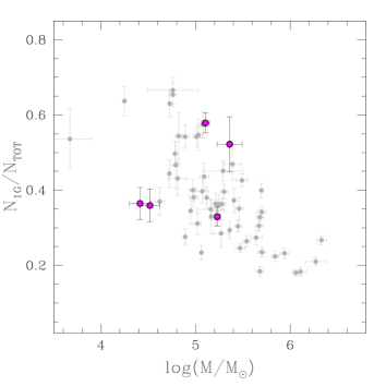
Figure 14: Fraction of 1G stars against the present-day cluster mass for Galactic GCs. Gray points indicate literature results (Milone et al., 2017a; Dondoglio et al., 2021), whereas magenta dots mark the clusters without previous studies on the ChM. Cluster masses are from Baumgardt & Hilker (2018).

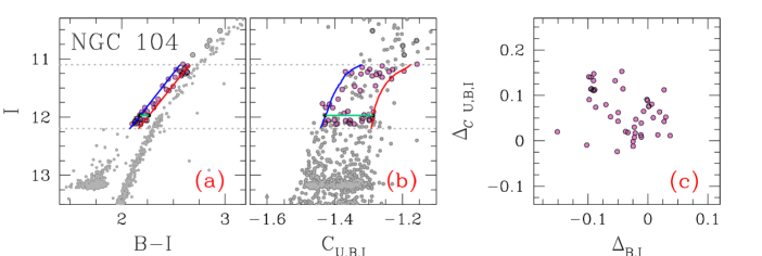
Figure 15: This figure illustrates the procedure to derive the ChM of AGB stars in NGC 104 (47 Tucanae). Panels a and b represent the $I$ vs. $B-I$ and $I$ vs. $C_{\rm U,B,I}$ diagrams, respectively. The red and blue lines mark the boundaries of the AGB sequence, while the aqua segments indicate the width of the AGB sequence. AGB stars are marked with dots. Only AGB stars between the two horizontal (pink dots) lines are used to derive the ChM plotted in panel c.

5 The chromosome map of AGB stars

The investigation of multiple populations along the AGB represents crucial test for stellar evolution. Stellar evolution models predict that most GC stars would evolve into the AGB phase, possibly, with the remarkable exception of 2G stars stars with extreme helium contents (e.g. Kippenhahn & Weigert, 1990; Landsman et al., 1996; Chantereau et al., 2016). This conclusion is challenged by spectroscopic work on multiple population, which reveal that some 2G stars with moderate helium enhancement skip the AGB phase (see e.g. Campbell et al., 2013; Johnson & Pilachowski, 2012; Johnson et al., 2015; Marino et al., 2017).

Recent works, based on HST photometry, have shown that ChMs are efficient tools to identify and characterize multiple populations along the AGB of GCs (Marino et al., 2017; Lagioia et al., 2021). In the following, we present the method to derive ChM of AGB stars from $U,B,I$ ground-based photometry.

Due to the small number of AGB stars in NGC 288, we use NGC 104 as a test case. The procedure is illustrated in Figure 15 and is similar to the method that we used for RGB stars. In a nutshell, we first selected by eye a sample of bona-fide AGB stars, based on their position in the $I$ vs. $B-I$ CMD (Figure 15a). The ChM is derived from the $I$ vs. $B-I$ and the $I$ vs. $C_{\rm U,B,I}$ diagrams shown in panels a and b of Figure 15. The red and blue boundaries of the AGB are derived by hand and are used to derive the $\Delta_{\rm B,I}$ and $\Delta c_{\rm{U,B,I}}$ pseudo colours by using Equations1 and 2. The values of $W_{\rm B,I}$ and $W_{C\rm U,B,I}$ correspond to the $B-I$ and $C_{\rm U,B,I}$ separations between the fiducial lines, calculated 5 $I$ mag above the main-sequence turnoff.

The resulting ChM for AGB stars in NGC 104 is plotted in panel c of Figure 15. Clearly, AGB stars comprise a group 1G stars that are distributed around the origin of the ChM and a group of 2G stars with large values of $\Delta c_{\rm{U,B,I}}$ and $\Delta_{\rm B,I}$. Noticeably, the fraction of 1G stars along the AGB is 58$\pm$5 % and is significantly larger than that derived from the ChM of RGB stars (40$\pm$1 %). This is in agreement with the spectroscopic study of NGC 104 from Johnson et al. (2015), where the fraction of Na-poor and Na-rich stars changes from 45:50 on the RGB to 63:37 on the AGB. Although this phenomenon still misses a definitive explanation, our results support the idea that 2G stars are affected by larger amounts of RGB mass loss than 1G stars (Campbell et al., 2013; Johnson et al., 2015; Tailo et al., 2015, 2020). It is also interesting to notice that the fractions of 1G inferred from wide-field photometry is much larger than that obtained from the traditional ChM in the central region (18$\pm$1 % from Milone et al., 2017a). This results is quite expected given that 2G stars of NGC 104 are more centrally concentrated than the 1G ones (Milone et al., 2012b; Cordero et al., 2014; Dondoglio et al., 2021). When we estimate the population ratio from the ground-based ChM of the stars in the HST field of view, we find a fraction of 1G stars of 21$\pm$3 %, in agreement with the values provided by the papers quoted above, in the same region.

6 Summary and conclusions

By far, the photometric catalogs provided by Peter Stetson have provided state-of-the-art photometry of GC stars from ground-based facilities (Stetson & Harris, 1988; Stetson, 2005; Stetson et al., 2019). We have analyzed photometry and astrometry of 43 GCs in the $U,B,V,$ and $I$ bands by Stetson et al. (2019) and combined them with stellar proper motions and parallaxes from Gaia eDR3 (Gaia Collaboration et al., 2021).

We identified bona-fide cluster members and estimated the amount of differential reddening in the field of view of each cluster and found that the maximum reddening variation ranges from $\Delta$E(B$-$V)$\sim 0.19$ mag to less than 0.01 mag. The amount of differential reddening correlates with the average reddening in the direction of the cluster. Nevertheless, clusters with similar values of E(B$-$V) can exhibit different amounts of differential reddening. We corrected the photometry of 18 GCs with significant variation of reddening and publicly release the differential-reddening catalogs.

Clearly, high-resolution reddening maps for GC cluster members have various astrophysical applications. As an example, applying the InfraRed Flux Method to better determine the effective-temperature scale of the RGB will have several implications for the study of stellar populations and stellar modelling (e.g. Salaris et al., 2018; Casagrande et al., 2021). In this work, we focus on the multiple-population phenomenon.

To investigate multiple populations from ground-based photometry, we started using NGC 288 as a test case. The reason for this choice is that NGC 288 is a quite simple cluster in the context of multiple populations, where 1G and 2G stars exhibit distinct sequences in the photometric diagrams that are commonly used to investigate the multiple populations (Piotto et al., 2013; Monelli et al., 2013; Milone et al., 2017a; Cordoni et al., 2020). The main results on NGC 288 can be summarized as follows.

• Based on the $I$ vs. $B-I$ CMD and the $I$ vs. $C_{\rm U,B,I}$ pseudo CMD of NGC 288, we built the $\Delta c_{\rm U,B,I}$ vs. $\Delta_{\rm B,I}$ ChM for RGB stars. The NGC 288 stars distribute into two main blobs in the ChM. We matched the catalog from Stetson et al. (2019) and from HST photometry (Milone et al., 2017a) to identify stars with both HST and ground-based photometry. We find that the 1G stars defined by Milone et al. (2017a) distribute around the origin of the $\Delta c_{\rm U,B,I}$ vs. $\Delta_{\rm B,I}$ ChM, while 2G stars exhibit large values of $\Delta c_{\rm U,B,I}$ and $\Delta_{\rm B,I}$. This is the first time that a ChM is derived from ground-based Johnson-Cousin photometry (see also the work by Hartmann et al. (2022) who derived the ChM from ground-based photometry, by using the $U$ band and the narrow-band filters centered around 3780Å  and 3950Å.).

• We also show that the $\Delta_{\rm U,B}$ vs. $\Delta_{\rm B,I}$ ChM, which is derived by the $I$ vs. $B-I$ and $I$ vs. $U-B$ CMDs, provides a clear separation between 1G and 2G stars.

• We used the values of [O/Fe], [Na/Fe], and [Fe/H] inferred by Carretta et al. (2009) from high-resolution spectroscopy to infer the chemical composition of the stellar populations identified on the ChM. We find that 1G stars and 2G stars have the same iron abundance ($\Delta$[Fe/H]_2G-1G=$-0.01\pm 0.01$). 2G stars are sodium enhanced ($\Delta$[Na/Fe]_2G-1G=$0.42\pm 0.04$) and depleted oxygen depleted ($\Delta$[O/Fe]_2G-1G=$-0.28\pm 0.09$) with respect to the 1G. This result is consistent with previous findings by Marino et al. (2019a) based on the HST ChM and the elemental abundances from Carretta et al. (2009). However, the largest field of view covered by the ground-based photometry used in this paper provides improved results. Indeed, we used larger samples of 1G and 2G stars for which spectroscopic estimates of chemical composition are available.

• We studied the radial distribution of stellar populations of NGC 288 and find that the fraction of 1G stars is consistent with a flat distribution. Similarly to NGC 288, the 1G and 2G stars of various GCs (e.g., NGC 6752, NGC 6362, M5, NGC 6366, NGC 6838 among the others Lee, 2017; Milone et al., 2019; Dalessandro et al., 2018; Dondoglio et al., 2021) share the same radial distribution. These observations are consistent with a scenario where both populations born with the same radial distributions. However, a lack of radial gradient of the population ratio is also expected in the scenarios where 2G stars form in the innermost cluster regions. These scenarios predict that the multiple populations of some clusters are fully mixed due to dynamical evolution (Vesperini et al., 2013).

  Results on NGC 288 are consistent with the scenario by Hénault-Brunet et al. (2015). Indeed, according to these authors (see their Figure 16), NGC 288 is on the edge between the evaporation and expansion dominated regions of the plot. A cluster that is in the expansion-dominated phase of its evolution is believed to be not fully mixed. On the contrary, clusters in the evaporation-dominated phase are believed to be completely relaxed and to have their populations mixed, after losing a large fraction of their initial mass. Therefore, NGC 288 might have reached a significant mixing between its stellar populations, explaining the observed flat radial distribution of the 1G fraction. NGC 104, on the other hand, is in the expansion-dominated phase of its evolution, therefore it still shows spatial and kinematic differences between the two populations, as shown in the radial distribution of NGC 104 (see Figure 19 of Dondoglio et al., 2021). This is also consistent with our finding that the fractions of 1G inferred from wide-field photometry is much larger than that obtained from the traditional ChM in the central region of NGC 104.

Driven by the results on NGC 288, we present the ChMs of 29 GCs, where the bulk of 1G and 2G stars can be distinguished in the ChM. Our sample comprises five Type I GCs, namely NGC 1904, NGC 4147, NGC 6712, NGC 7006 and Palomar 11, without previous determinations of ChMs. For these clusters, we calculated the fraction of 1G stars and find that they follow the same relation with cluster mass as the other studied Galactic GCs.

The atlas of 29 ChMs reveals that the extensions of the 1G and 2G sequences as well as the relative numbers of 1G and 2G stars change from one cluster to another. We thus confirm that multiple populations exhibit a large degree of variety (see also Renzini et al., 2015; Milone et al., 2017a, 2020a). Moreover, the ground-based ChMs allow to disentangle between Type I and Type II GCs. Indeed, the latter exhibit a ChM sequence with large $\Delta_{\rm B,I}$ values that run on the right side of the main ChM.

We find that the 1G sequences of several GCs (e.g. NGC 5927, NGC 6366, NGC 104, NGC 6838, NGC 6712, NGC 5272, NGC 6254, NGC 3201, and NGC 4833) are clearly elongated in the $\Delta c_{\rm U,B,I}$ vs. $\Delta_{\rm B,I}$ ChM, whereas the other GCs show less-extended 1G sequences along the abscissa of the ChM. We thus confirm the recent discoveries of extended 1G sequences in the ChM and corroborate the conclusion that the pristine material from which GC formed was not chemically homogeneous (Milone et al., 2015, 2017a; Cabrera-Ziri et al., 2019; Legnardi et al., 2022).

Based on high-resolution spectroscopy and HST multi-band photometry, the presence of star-to-star metallicity variations seems the most plausible explanation for the 1G extended sequence (Marino et al., 2019a; Kamann et al., 2020; Legnardi et al., 2022). Helium variations and stellar binarity have been considered as alternative solutions, but they do not seem to fully reproduce the observations (Milone et al., 2018; Marino et al., 2019a; Kamann et al., 2020).

The ChMs provided in this paper provide further constraints of the chemical composition of 1G stars. We discovered that the 1G sequence of some clusters like NGC 6366 and NGC 6838 is thicker than the 2G sequence along the $\Delta c_{\rm U,B,I}$ direction. Moreover, the slope of the 1G sequence of NGC 104 and NGC 5927 have positive slopes in the $\Delta c_{\rm U,B,I}$ vs. $\Delta_{\rm B,I}$, in contrast with what is observed in the remaining GCs with extended 1G.

In summary, results on NGC 288 and on the other studied clusters demonstrate that the $\Delta c_{\rm U,B,I}$ vs. $\Delta_{\rm B,I}$ ChM is an efficient tool to identify and characterize multiple populations in GCs from ground-based photometry. The ChMs that we have introduced can be obtained from photometry from wide-field facilities. This fact allows us to overcome the main limitations on the study of multiple-populations that were associated with the small field of view of the HST cameras.

Table 3: This table lists for each cluster the values of the 68^th percentile, $\sigma_{\Delta E(B-V)}$, the difference between the 98^th and the 2^nd percentile of differential-reddening distributions, and the value of 68^th percentile of $\Delta E(B-V)_{\rm B-I}$ - $\Delta E(B-V)_{\rm U-V}$. The maximum radial distance used to derive differential reddening and the radius range used to build the ChM from cluster center of the region, $R_{\rm max}$ and R_ChM, are also provided.

ID	$\sigma_{\Delta E(B-V)}$	$\Delta E(B-V)_{\rm 98\%-2\%}$	$\sigma_{\rm(\Delta E(B-V)_{\rm B-I}-\Delta E(B-V)_{\rm U-V})}$	$R_{\rm max}$	RChM
	[mag]	[mag]	[mag]	[arcmin]	[arcmin]
NGC 104	0.005 $\pm$0.001	0.021 $\pm$ 0.001	0.008	16.9	0.0 - 16.9
NGC 288	0.003 $\pm$0.001	0.010 $\pm$ 0.001	0.003	10.3	0.8 - 10.3
NGC 1261	0.005 $\pm$0.001	0.018 $\pm$ 0.002	0.006	5.1	0.0 - 5.1
NGC 1851	0.004 $\pm$0.001	0.014 $\pm$ 0.004	0.005	8.4	1.2 - 8.4
NGC 1904	0.006 $\pm$0.002	0.020 $\pm$ 0.007	0.007	6.8	1.5 - 6.8
NGC 2298	0.014 $\pm$0.002	0.049 $\pm$ 0.005	0.009	4.2	0.9 - 4.2
NGC 2808	0.013 $\pm$0.002	0.049 $\pm$ 0.009	0.009	6.8	0.0 - 6.8
NGC 3201	0.036 $\pm$0.003	0.134 $\pm$ 0.013	0.009	7.7	1.2 - 7.7
NGC 4147	0.003 $\pm$0.001	0.008 $\pm$ 0.001	0.003	3.4	0.0 - 3.4
NGC 4372	0.054 $\pm$0.003	0.187 $\pm$ 0.021	0.016	8.4	$-$
NGC 4590	0.004 $\pm$0.001	0.013 $\pm$ 0.002	0.004	6.7	0.0 - 6.7
NGC 4833	0.038 $\pm$0.003	0.138 $\pm$ 0.011	0.015	6.9	0.0 - 6.9
NGC 5024	0.003 $\pm$0.001	0.013 $\pm$ 0.002	0.005	9.2	$-$
NGC 5053	0.002 $\pm$0.001	0.008 $\pm$ 0.001	0.001	6.9	0.7 - 6.9
NGC 5272	0.004 $\pm$0.001	0.015 $\pm$ 0.003	0.008	12.0	2.3 - 12.0
NGC 5286	0.023 $\pm$0.004	0.091 $\pm$ 0.015	0.013	4.2	$-$
NGC 5634	0.006 $\pm$0.001	0.016 $\pm$ 0.003	0.004	5.0	$-$
NGC 5904	0.004 $\pm$0.001	0.014 $\pm$ 0.002	0.007	11.9	2.6 - 11.9
NGC 5927	0.040 $\pm$0.004	0.141 $\pm$ 0.010	0.018	5.1	1.6 - 5.1
NGC 5986	0.020 $\pm$0.002	0.070 $\pm$ 0.007	0.017	4.3	$-$
NGC 6101	0.007 $\pm$0.001	0.026 $\pm$ 0.004	0.010	7.1	$-$
NGC 6121	0.020 $\pm$0.001	0.088 $\pm$ 0.008	0.013	6.8	0.4 - 6.8
NGC 6205	0.003 $\pm$0.001	0.013 $\pm$ 0.001	0.004	10.9	3.3 - 10.9
NGC 6218	0.008 $\pm$0.001	0.029 $\pm$0.003	0.006	6.7	1.6 - 6.7
NGC 6254	0.018 $\pm$0.003	0.071 $\pm$0.006	0.010	10.8	0.0 - 10.8
NGC 6341	0.003 $\pm$0.001	0.011 $\pm$0.001	0.003	8.4	$-$
NGC 6366	0.029 $\pm$0.003	0.101 $\pm$0.007	0.009	6.9	0.0 - 6.9
NGC 6656	0.020 $\pm$0.003	0.082 $\pm$0.015	0.019	8.4	$-$
NGC 6712	0.026 $\pm$0.001	0.079 $\pm$0.013	0.010	8.5	0.8 - 8.5
NGC 6752	0.005 $\pm$0.001	0.016 $\pm$0.001	0.003	8.5	0.9 - 8.5
NGC 6760	0.050 $\pm$0.008	0.160 $\pm$0.025	0.015	3.4	$-$
NGC 6809	0.006 $\pm$0.001	0.021 $\pm$0.002	0.009	10.9	2.1 - 10.9
NGC 6838	0.019 $\pm$0.002	0.077 $\pm$0.007	0.005	3.5	0.0 - 3.5
NGC 6934	0.006 $\pm$0.001	0.023 $\pm$0.004	0.006	3.3	0.0 - 3.3
NGC 6981	0.004 $\pm$0.001	0.016 $\pm$0.001	0.004	5.3	0.5 - 5.3
NGC 7006	0.003 $\pm$ 0.001	0.010 $\pm$ 0.001	0.002	3.2	0.0 - 3.2
NGC 7078	0.009 $\pm$ 0.001	0.032 $\pm$ 0.003	0.005	8.4	$-$
NGC 7089	0.004 $\pm$ 0.001	0.016 $\pm$ 0.002	0.003	8.4	1.6 - 8.4
NGC 7099	0.003 $\pm$ 0.001	0.010 $\pm$ 0.002	0.007	8.1	$-$
NGC 7492	0.002 $\pm$ 0.001	0.005 $\pm$ 0.002	0.002	3.4	0.0 - 3.4
IC 4499	0.004 $\pm$ 0.001	0.017 $\pm$ 0.003	0.003	6.6	$-$
Palomar 11	0.018 $\pm$ 0.003	0.054 $\pm$ 0.009	0.008	2.8	$-$
Terzan 8	0.003 $\pm$ 0.001	0.016 $\pm$ 0.002	0.005	5.1	$-$

Table 4: Fraction of 1G stars for the five GCs without previous determinations of the ChMs

ID	N1G/NTOT	Nstars
NGC 1904	0.33 $\pm$ 0.03	319
NGC 4147	0.36 $\pm$ 0.04	92
NGC 6712	0.58 $\pm$ 0.03	304
NGC 7006	0.52 $\pm$ 0.07	55
NGC 7492	0.36 $\pm$ 0.04	117

Data Availability

The data underlying this article will be shared on reasonable request to the corresponding author.

References

- Anderson et al. (2008) Anderson J., et al., 2008, AJ, 135, 2055
- Bastian et al. (2013) Bastian N., Lamers H. J. G. L. M., de Mink S. E., Longmore S. N., Goodwin S. P., Gieles M., 2013, MNRAS, 436, 2398
- Bastian et al. (2018) Bastian N., Kamann S., Cabrera-Ziri I., Georgy C., Ekström S., Charbonnel C., de Juan Ovelar M., Usher C., 2018, MNRAS, 480, 3739
- Baumgardt & Hilker (2018) Baumgardt H., Hilker M., 2018, MNRAS, 478, 1520
- Cabrera-Ziri et al. (2019) Cabrera-Ziri I., Lardo C., Mucciarelli A., 2019, MNRAS, 485, 4128
- Campbell et al. (2013) Campbell S. W., et al., 2013, Nature, 498, 198
- Carretta et al. (2009) Carretta E., et al., 2009, A&A, 505, 117
- Carretta et al. (2011) Carretta E., Bragaglia A., Gratton R., D’Orazi V., Lucatello S., 2011, A&A, 535, A121
- Carretta et al. (2018) Carretta E., Bragaglia A., Lucatello S., Gratton R. G., D’Orazi V., Sollima A., 2018, A&A, 615, A17
- Casagrande et al. (2021) Casagrande L., et al., 2021, MNRAS, 507, 2684
- Chantereau et al. (2016) Chantereau W., Charbonnel C., Meynet G., 2016, A&A, 592, A111
- Cordero et al. (2014) Cordero M. J., Pilachowski C. A., Johnson C. I., McDonald I., Zijlstra A. A., Simmerer J., 2014, ApJ, 780, 94
- Cordoni et al. (2018) Cordoni G., Milone A. P., Marino A. F., Di Criscienzo M., D’Antona F., Dotter A., Lagioia E. P., Tailo M., 2018, ApJ, 869, 139
- Cordoni et al. (2020) Cordoni G., Milone A. P., Mastrobuono-Battisti A., Marino A. F., Lagioia E. P., Tailo M., Baumgardt H., Hilker M., 2020, ApJ, 889, 18
- D’Antona et al. (2016) D’Antona F., Vesperini E., D’Ercole A., Ventura P., Milone A. P., Marino A. F., Tailo M., 2016, MNRAS, 458, 2122
- D’Ercole et al. (2008) D’Ercole A., Vesperini E., D’Antona F., McMillan S. L. W., Recchi S., 2008, MNRAS, 391, 825
- Dalessandro et al. (2018) Dalessandro E., et al., 2018, ApJ, 864, 33
- Dalessandro et al. (2019) Dalessandro E., et al., 2019, ApJ, 884, L24
- Decressin et al. (2007) Decressin T., Meynet G., Charbonnel C., Prantzos N., Ekström S., 2007, A&A, 464, 1029
- Denissenkov & Hartwick (2014) Denissenkov P. A., Hartwick F. D. A., 2014, MNRAS, 437, L21
- Dondoglio et al. (2021) Dondoglio E., Milone A. P., Lagioia E. P., Marino A. F., Tailo M., Cordoni G., Jang S., Carlos M., 2021, ApJ, 906, 76
- Dotter et al. (2008) Dotter A., Chaboyer B., Jevremović D., Kostov V., Baron E., Ferguson J. W., 2008, ApJS, 178, 89
- Gaia Collaboration et al. (2021) Gaia Collaboration et al., 2021, A&A, 649, A1
- Gieles et al. (2018) Gieles M., et al., 2018, MNRAS, 478, 2461
- Gratton et al. (2019) Gratton R., Bragaglia A., Carretta E., D’Orazi V., Lucatello S., Sollima A., 2019, A&ARv, 27, 8
- Grundahl et al. (1998) Grundahl F., VandenBerg D. A., Andersen M. I., 1998, ApJ, 500, L179
- Harris (1996) Harris W. E., 1996, AJ, 112, 1487
- Hartmann et al. (2022) Hartmann E. A., et al., 2022, MNRAS, 515, 4191
- Hénault-Brunet et al. (2015) Hénault-Brunet V., Gieles M., Agertz O., Read J. I., 2015, MNRAS, 450, 1164
- Jang & Lee (2015) Jang S., Lee Y.-W., 2015, ApJS, 218, 31
- Jang et al. (2014) Jang S., Lee Y. W., Joo S. J., Na C., 2014, MNRAS, 443, L15
- Jang et al. (2021) Jang S., et al., 2021, ApJ, 920, 129
- Johnson & Pilachowski (2012) Johnson C. I., Pilachowski C. A., 2012, ApJ, 754, L38
- Johnson et al. (2015) Johnson C. I., et al., 2015, AJ, 149, 71
- Kamann et al. (2020) Kamann S., et al., 2020, A&A, 635, A65
- Kippenhahn & Weigert (1990) Kippenhahn R., Weigert A., 1990, Stellar Structure and Evolution
- Kurucz (1970) Kurucz R. L., 1970, SAO Special Report, 309
- Kurucz (2005) Kurucz R. L., 2005, Memorie della Societa Astronomica Italiana Supplementi, 8, 14
- Kurucz & Avrett (1981) Kurucz R. L., Avrett E. H., 1981, SAO Special Report, 391
- Lagioia et al. (2019) Lagioia E. P., Milone A. P., Marino A. F., Dotter A., 2019, ApJ, 871, 140
- Lagioia et al. (2021) Lagioia E. P., et al., 2021, ApJ, 910, 6
- Landolt (1992) Landolt A. U., 1992, AJ, 104, 340
- Landsman et al. (1996) Landsman W. B., Sweigart A. V., Bohlin R. C., Neff S. G., O’Connell R. W., Roberts M. S., Smith A. M., Stecher T. P., 1996, ApJ, 472, L93
- Larsen et al. (2019) Larsen S. S., Baumgardt H., Bastian N., Hernandez S., Brodie J., 2019, A&A, 624, A25
- Lee (2017) Lee J.-W., 2017, ApJ, 844, 77
- Lee & Jang (2016) Lee Y.-W., Jang S., 2016, ApJ, 833, 236
- Lee et al. (1999) Lee Y. W., Joo J. M., Sohn Y. J., Rey S. C., Lee H. C., Walker A. R., 1999, Nature, 402, 55
- Legnardi et al. (2022) Legnardi M. V., et al., 2022, MNRAS, 513, 735
- Marino et al. (2008) Marino A. F., Villanova S., Piotto G., Milone A. P., Momany Y., Bedin L. R., Medling A. M., 2008, A&A, 490, 625
- Marino et al. (2017) Marino A. F., et al., 2017, ApJ, 843, 66
- Marino et al. (2019a) Marino A. F., et al., 2019a, MNRAS, 487, 3815
- Marino et al. (2019b) Marino A. F., et al., 2019b, ApJ, 887, 91
- Milone & Marino (2022) Milone A. P., Marino A. F., 2022, Universe, 8, 359
- Milone et al. (2010) Milone A. P., et al., 2010, ApJ, 709, 1183
- Milone et al. (2012a) Milone A. P., et al., 2012a, A&A, 540, A16
- Milone et al. (2012b) Milone A. P., et al., 2012b, ApJ, 744, 58
- Milone et al. (2015) Milone A. P., et al., 2015, MNRAS, 447, 927
- Milone et al. (2017a) Milone A. P., et al., 2017a, MNRAS, 464, 3636
- Milone et al. (2017b) Milone A. P., et al., 2017b, MNRAS, 469, 800
- Milone et al. (2018) Milone A. P., et al., 2018, MNRAS, 481, 5098
- Milone et al. (2019) Milone A. P., et al., 2019, MNRAS, 484, 4046
- Milone et al. (2020a) Milone A. P., et al., 2020a, MNRAS, 491, 515
- Milone et al. (2020b) Milone A. P., et al., 2020b, MNRAS, 497, 3846
- Monelli et al. (2013) Monelli M., et al., 2013, MNRAS, 431, 2126
- Niederhofer et al. (2017) Niederhofer F., et al., 2017, MNRAS, 465, 4159
- Piotto et al. (2013) Piotto G., Milone A. P., Marino A. F., Bedin L. R., Anderson J., Jerjen H., Bellini A., Cassisi S., 2013, ApJ, 775, 15
- Piotto et al. (2015) Piotto G., et al., 2015, AJ, 149, 91
- Renzini et al. (2015) Renzini A., et al., 2015, MNRAS, 454, 4197
- Renzini et al. (2022) Renzini A., Marino A. F., Milone A. P., 2022, MNRAS, 513, 2111
- Salaris et al. (2018) Salaris M., Cassisi S., Schiavon R. P., Pietrinferni A., 2018, A&A, 612, A68
- Sbordone et al. (2004) Sbordone L., Bonifacio P., Castelli F., Kurucz R. L., 2004, Memorie della Societa Astronomica Italiana Supplementi, 5, 93
- Sbordone et al. (2007) Sbordone L., Bonifacio P., Castelli F., 2007, in Kupka F., Roxburgh I., Chan K. L., eds, IAU Symposium Vol. 239, Convection in Astrophysics. pp 71–73, doi:10.1017/S1743921307000142
- Schlegel et al. (1998) Schlegel D. J., Finkbeiner D. P., Davis M., 1998, ApJ, 500, 525
- Stetson (2005) Stetson P. B., 2005, PASP, 117, 563
- Stetson & Harris (1988) Stetson P. B., Harris W. E., 1988, AJ, 96, 909
- Stetson et al. (2019) Stetson P. B., Pancino E., Zocchi A., Sanna N., Monelli M., 2019, MNRAS, 485, 3042
- Tailo et al. (2015) Tailo M., et al., 2015, Nature, 523, 318
- Tailo et al. (2020) Tailo M., et al., 2020, MNRAS, 498, 5745
- Vanderbeke et al. (2015) Vanderbeke J., De Propris R., De Rijcke S., Baes M., West M., Alonso-García J., Kunder A., 2015, MNRAS, 451, 275
- Vesperini et al. (2013) Vesperini E., McMillan S. L. W., D’Antona F., D’Ercole A., 2013, MNRAS, 429, 1913
- Wang et al. (2020) Wang L., Kroupa P., Takahashi K., Jerabkova T., 2020, MNRAS, 491, 440
- Yong & Grundahl (2008) Yong D., Grundahl F., 2008, ApJ, 672, L29
- Zennaro et al. (2019) Zennaro M., Milone A. P., Marino A. F., Cordoni G., Lagioia E. P., Tailo M., 2019, MNRAS, 487, 3239
- de Mink et al. (2009) de Mink S. E., Pols O. R., Langer N., Izzard R. G., 2009, A&A, 507, L1