Estimating phase transition of perturbed $J_{1}-J_{2}$ Heisenberg quantum chain
in mixtures of ground and first excited states

Abstract

We show that the nearest neighbour entanglement in a mixture of ground and first excited states - a subjacent state - of the $J_{1}-J_{2}$ Heisenberg quantum spin chain can be used as an order parameter to detect the phase transition of the chain from a gapless spin fluid to a gapped dimer phase. We study the effectiveness of the order parameter for varying relative mixing probabilities between the ground and first excited states in the subjacent state for different system sizes, and extrapolate the results to the thermodynamic limit. We observe that the nearest neighbour concurrence can play a role of a good order parameter even if the system is in the ground state, but with a small finite probability of leaking into the first excited state. Moreover, we apply the order parameter of the subjacent state to investigate the response to separate introductions of anisotropy and of glassy disorder on the phase diagram of the model, and analyse the corresponding finite-size scale exponents and the emergent tricritical point in the former case. The anisotropic $J_{1}-J_{2}$ chain has a richer phase diagram which is also clearly visible by using the same order parameter.

I Introduction

The study of quantum many-body systems utilizing the concepts of quantum information theory is a fruitful avenue for investigating various many-body quantum phenomena like quantum phase transitions [1, 2, 3, 4, 5]. Investigations in this direction include Refs. [6, 7], wherein bipartite quantum entanglement [8, 9, 10] was used as an order parameter for detection of the quantum phase transition in the one-dimensional transverse Ising and other XY quantum spin models. Later on, multipartite quantum entanglement measures like geometric [11, 12, 13, 10] and generalized geometric measure  [14, 15], and other quantum correlation measures like quantum discord [16, 17], have been shown to be effective detectors of quantum phase transitions in many-body quantum systems. See e.g. Refs. [18, 19, 20, 21, 22, 23, 24, 25, 26, 27, 28, 29, 30, 31, 32, 33] and Refs. [34, 35] in this regard. A strong connection between entanglement and many body physics has been established by the numerical simulation of quantum many-body systems using matrix product states [36, 37, 38], projected entangled pair states [39], density matrix renormalization group [40, 41, 42, 39, 43], tensor network states [44, 45, 46, 47, 48, 49], etc. Experimental evidence of these and related concepts in quantum many-body systems are found in atoms in an optical lattice [50, 51], trapped ions [52, 53], photons  [54], and nuclear magnetic resonance systems  [55] of particles. Furthermore, the connection between quantum information theory and many-body quantum systems helps in quantum state engineering which facilitates the development of realistic quantum computation.

The phenomenon of quantum phase transition in the $J_{1}-J_{2}$ Heisenberg spin model, where $J_{1}$ and $J_{2}$ stand for the nearest and next to nearest neighbour coupling constants respectively, is a well known one. See e.g.  [56, 57, 58, 59, 60]. Classically, phase transitions occur when the system approaches a certain critical temperature, beyond which the macroscopic properties of the system change [61, 62, 63, 64]. Quantum phase transitions take place at absolute zero temperature, when some external parameter or coupling strength is varied [1, 4, 65]. The quantum phase transition of the one-dimensional antiferromagnetic $J_{1}-J_{2}$ model from a gapless fluid to gapped dimer phase was investigated in [66, 67, 68, 69, 70] using exact digonalization and field theory formalism. Subsequently, measures of bipartite entanglement, like concurrence [71, 72], quantum fidelity [73], and valence bond entanglement [74] have been shown to be good detectors of the quantum phase transition, considering the respective quantities in the first excited state, but not in the ground state [75, 76]. The measure of multipartite entanglement, generalized geometric measure, also could not indicate the quantum phase transition while considering the ground state [33].

Quantum systems are usually prone to noise from the environment. One of the most common forms of noise is thermal noise, and a many-body system prepared at very low temperatures, is practically a mixture of its low-lying energy states. The study of critical phenomena and quantum information measures of such systems are extensively done for the ground state. It is however interesting to study other low-lying states as well, as the system can only be in the ground state at the absolute zero temperature, which is not practical.

In this paper, we show that the nearest neighbour concurrence of a mixture of ground and first excited states of the one-dimensional quantum Heisenberg $J_{1}-J_{2}$ model can behave as a good indicator of the quantum phase transition in the model. We consider a mixture of the ground and first excited states to mimic the state of the system at some finite temperature - the higher excited states, being present with lower probabilities, are ignored. We find that the two-party entanglement of such a state indicates the presence of the critical point in the ground state of the model. We are therefore trying to find “shadows” of the ground state quantum phase transitions in a given physical system, in states of the same system which have a finite but low temperature. This is physically meaningful, as a real state of a system will always be of the latter type. Although the concept of using a mixture of ground and first excited states and identifying entanglement as a good order parameter of phase transition in this model are already studied in the literature, in this paper we try to investigate this matter more deeply. Recently, concurrence [71, 72] and shared purity [77], have been shown to be good quantum phase transition indicators in a mixture of ground and low-lying energy states for the $J_{1}-J_{2}$ model on a spin chain [78]. In that work, they have considered the mixture of ground and low-lying energy states with certain mixing probabilities. On the contrary, in this paper we find that for arbitrarily small mixing probabilities also, the critical point can be observed. Furthermore, we investigate the effect of mixing probabilities on the phase transition points for different system-sizes and a finite-size scaling analysis is done to find the critical point in the thermodynamic limit. Moreover, we analyse the effect of introduction of an anisotropy parameter in the nearest neighbour and next-nearest neighbour coupling constants of the system and in particular investigate the change in the phase transition point on varying the anisotropy parameter. A scaling analysis is done here as well. A phase diagram of the system is clearly visible for this case. From the depictions given in this paper, we can see the phase boundaries among the various phases of the system like spin fluid state, dimer phase and Néel phase. In previous works, the phase boundaries were obtained using various methods like level-spectroscopy [79] and tensor network methods [80]. In this work, we obtain a similar phase boundary, using nearest-neighbour concurrence. We reiterate here that quantum phase transitions happen only at zero temperature, and so the studies of finite low-temperature states or low-lying eigenstates detect the traces of zero-temperature transitions that are still visible in a state that is not a zero-temperature state.

In practical scenarios, it is neither possible to reach absolute zero-temperature nor is it possible to completely isolate our system from the environment. This makes it quite difficult to fabricate a lattice chain with $N$ quantum spin$-\frac{1}{2}$ particles. There may arise fluctuations in the positions of the spins in the lattice or in the tuning parameters of the set-up, or the magnetic field may not be homogeneous. These imperfections are very difficult to keep track of and are usually modelled as disorder. It is therefore both natural and potentially useful to study the effect of disorder in our system. Sometimes, the presence of disorder may provide some advantages over the ideal situation  [81, 82, 83, 84, 85, 86, 87, 88, 89, 90, 91, 92, 93, 94, 95, 96, 97, 98, 99, 100, 101, 102, 103, 104, 105, 106, 107, 108, 109, 110, 111, 112, 113, 114, 115, 116, 117, 118, 119, 120, 121, 122, 123, 124, 125, 126, 127, 128, 129]. This type of disordered system is more realistic and we show that entanglement still behaves as an identifier of phase transition even if the system is some distance away from its ideal disorder-free nature. In our work, we introduce a disorder parameter in the system and obtain the shifts in the critical point of the system in the presence of glassy Gaussian disorder.

The remainder of the paper is arranged as follows. The one-dimensional $J_{1}-J_{2}$ Heisenberg spin model and the definition of the quantum information order parameter, concurrence, is discussed in Sec. II. The behaviour of nearest neighbour concurrence, especially its dependence on the mixing probability of ground and first excited states is presented in Sec. III. A finite-size scaling for the extrapolation of the results in the thermodynamic limit is also presented in this section. In Sec. IV, we introduce an anisotropy parameter in the system and note the shift of the phase transition point depending on the parameter and extrapolate the result to the thermodynamic limit. Section V contains the behaviour of nearest neighbour concurrence in the presence of glassy Gaussian disorder. The concluding remarks are presented in Sec. VI.

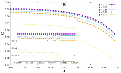
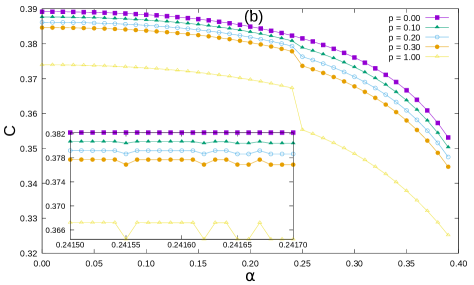
Figure 1: Nearest neighbour concurrence of the $J_{1}-J_{2}$ model. The concurrence between two consecutive spin particles is plotted with respect to the relative coupling strength $\alpha$ for different values of $p$ of the subjacent state for (a) $N=20$ and (b) $N=24$. The regions near the transition points are magnified and shown in the respective insets. The different colors of the lines with the different symbols represent the different values of $p$, which are mentioned in the legends. The quantity plotted along the horizontal axes is dimensionless, whereas the same along the vertical axes are in ebits.

II Motivating the choice of system state

The one-dimensional $J_{1}-J_{2}$ Heisenberg spin model, having the nearest and next-nearest neighbour coupling constants as $J_{1}$ and $J_{2}$ respectively, can be described by the Hamiltonian,

$$H=J_{1}\hbar\sum_{i=1}^{N}{\vec{\sigma}_{i}\cdot\vec{\sigma}_{i+1}}+J_{2}\hbar\sum_{i=1}^{N}{\vec{\sigma}_{i}\cdot\vec{\sigma}_{i+2}},$$ (1)

with $N$ being the number of spins of the system and $\vec{\sigma}=\sigma^{x}\hat{x}+\sigma^{y}\hat{y}+\sigma^{z}\hat{z}$, where $\sigma^{x}$, $\sigma^{y}$ and $\sigma^{z}$ represent the Pauli matrices. Here we employ periodic boundary conditions, which means that $\vec{\sigma}_{N+1}=\vec{\sigma}_{1}$. Here $J_{1}\hbar$ and $J_{2}\hbar$, having the unit of energy, stand for the anti-ferromagnetic coupling constants and are therefore zero or positive real numbers. This model can describe some solid state systems like SrCuO₂ [130]. This model is also known as the Majumdar–Ghosh model for $\alpha=\frac{J_{2}}{J_{1}}=\frac{1}{2}$ [56]. At $\alpha=\frac{1}{2}$, the model is exactly solvable and the ground state is doubly degenerate. The quantum phase transition of the one-dimensional antiferromagnetic $J_{1}-J_{2}$ model from a gapless fluid to gapped dimer phase driven by the change of the system parameter $\alpha$ was investigated in [66, 67, 68, 69] using exact digonalisation and field theory formalism. It was found that the phase transition occurs around a critical value of the parameter, $\alpha_{c}\approx 0.241$. The anisotropic $J_{1}-J_{2}$ Heisenberg quantum spin model with an anisotropic coupling constant $\delta$ along the $z$ direction was studied in [131, 132, 133, 134]. When $\alpha\lesssim 0.24$, for $\delta<1$, the system is in the spin fluid phase and for $\delta>1$, it goes into the Néel phase. In the spin fluid phase, no ordered arrangement of spins is formed, and they remain fluctuating even at absolute zero temperature [135, 136]. Néel order phase is an antiferromagnetic phase below a sufficiently low temperature (known as Néel temperature) [137, 138]. The phase diagram of this model in the range $0\leq\alpha\leq\frac{1}{2}$ for $\delta\geq 0$ and $\delta\leq 0$ is studied in [139, 133]. The anisotropy constant $\delta$ plays an important role in the phase diagram of this model between $0\leq\alpha\leq\frac{1}{2}$, and so it is important to study the effect of this anisotropy term on the "isotropic" phase transition from gapless fluid to gapped dimer phase around $\alpha_{c}\approx 0.241$.

In the literature, the phase transition point was investigated by determining the difference between the singlet-triplet and the singlet-singlet energy gaps for finite-size systems [67, 68]. The singlet-triplet and singlet-singlet energy gaps are respectively given by

$$G_{st}(N,\alpha) = E_{1}^{(0)}(N,\alpha)-E_{0}^{(0)}(N,\alpha),$$

$$G_{ss}(N,\alpha) = E_{0}^{(1)}(N,\alpha)-E_{0}^{(0)}(N,\alpha).$$

$E_{m}^{(0)}(N,\alpha)$ and $E_{m}^{(l)}(N,\alpha)$ are respectively the ground and the $l^{th}$ excited state energies in the total spin angular momentum, $S_{total}=m$ subspace. The measures of bipartite entanglement, like concurrence [71, 72], and quantum fidelty [73] have been shown to be good detectors of the quantum phase transition, considering the respective quantities in the first excited state, but not in the ground state [75, 76]. So, while the phase transition at $\alpha\approx 0.2411$ is a zero-temperature phenomenon at the ground state, there could exist order parameters that find their shadows in the first excited state instead of the ground state. The measure of multipartite entanglement, generalized geometric measure, also could not indicate the quantum phase transition while considering the ground state [33]. Thus, concurrence, a measure of two-qubit entanglement, can be considered as an order parameter for detecting the phase transition of the $J_{1}-J_{2}$ model, not in the ground state but in the first excited state [75] as well as in a mixture of ground and some low-lying energy states [78].

For a two-qubit density matrix, the concurrence $C$ is defined as

$$C=\max(0,\sqrt{\lambda_{1}}-\sqrt{\lambda_{2}}-\sqrt{\lambda_{3}}-\sqrt{\lambda_{4}}),$$ (2)

where $\lambda_{i}$’s are the eigenvalues of $\rho\tilde{\rho}$ with $\lambda_{1}$ being the largest. Here, $\tilde{\rho}=(\sigma_{y}\otimes\sigma_{y})\rho^{*}(\sigma_{y}\otimes\sigma_{y})$ and $\rho^{*}$ is the complex conjugate of $\rho$ in the computational basis. In this paper, we consider mixtures of the ground and first excited states and investigate whether its concurrence acts as a good order parameter. We consider a situation where there is a possibility of the spins to be in the first excited state of the Hamiltonian with probability $p$ and the ground state of the same with probability $(1-p)$. Here we take $p$ as the probability corresponding to the Maxwell-Boltzmann distribution, viz. $p=\frac{e^{-\frac{E^{(1)}(N,\alpha)-E^{(0)}(N,\alpha)}{k_{B}T}}}{1+e^{-\frac{E^{(1)}(N,\alpha)-E^{(0)}(N,\alpha)}{k_{B}T}}}$, where $k_{B}$ is the Boltzmann constant and $T$ is the absolute temperature of the system. Here we have omitted the subscipts $m$ of $E$’s, as all energies are considered in the calculations. A periodic boundary condition is imposed on the system, i.e., $\sigma_{N+1}=\sigma_{1}$. The quantum state being considered can therefore be represented as

$$\rho=(1-p)|\Psi_{0}\rangle\langle\Psi_{0}|+\frac{p}{d}\sum_{i=1}^{d}|\Psi_{1}^{i}\rangle\langle\Psi_{1}^{i}|,$$ (3)

where $|\Psi_{0}\rangle$ is the ground state and $|\Psi_{1}^{i}\rangle$s are the first excited states with $d$-fold degeneracy. We will refer to this as the subjacent state. We have only considered systems with even number of spins, for this the ground state has no degeneracy. The motivation behind considering the subjacent state is that a physical system at non-zero temperature, will be in a thermal mixture of the eigenstates of the system and for very low temperatures, the ground state and first excited states will have considerably higher probability than the other excited states. In fact, for every small $p$, we can find a non zero finite temperature which corresponds to the probability distribution between the first excited state and ground state. In this paper we are restricting ourselves to small values of $p$, vis-á-vis low but non-zero temperatures, as for higher temperatures, higher energy states will also contribute which we are ignoring. For the numerical analysis, the ground and first excited states of the system are obtained by using the Lanczos method [140] of exact diagonalisation. The concurrence we obtain in the paper is the concurrence of two consecutive spins. Due to the symmetry of the Hamiltonian, and as we are imposing periodic boundary condition, the entanglement between any two nearest neighbour spins will be the same. In the succeeding sections, "concurrence" refers to the nearest neighbour concurrence. In the succeeding section, we investigate how the behaviour of concurrence as an order parameter depends on the values of $p$, for the $J_{1}-J_{2}$ model.

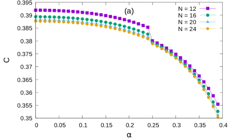
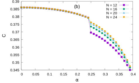
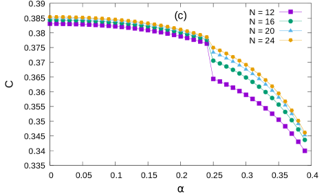
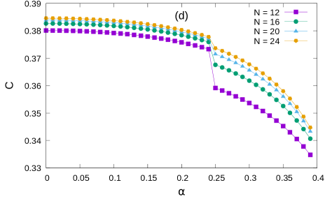
Figure 2: Nearest neighbour concurrence of the $J_{1}-J_{2}$ model for different system sizes. Here we have depicted the nearest neighbour concurrence with relative coupling $\alpha$ for different values of $N$, for (a) $p=0.10$, (b) $p=0.20$, (c) $p=0.25$ and (d) $p=0.30$ of the subjacent state. The different colors of the lines with different symbols represent different values of $N$, which are mentioned in the legends. The quantity plotted along the horizontal axes is dimensionless and the same along the vertical axes is in ebits.

III Concurrence of subjacent state as order parameter in $J_{1}-J_{2}$ model

The behaviour of concurrence as an order parameter strongly depends on the mixing probability $p$ of the ground and the first excited states. In Fig. 1, we depict the nature of concurrence with the relative coupling strength $\alpha$ for different values of mixing probability $p$ for $N=20$ and $N=24$, in the $J_{1}-J_{2}$. As already known, we observe that the nearest neighbor concurrence of the ground state ($p=0$) does not show any discontinuity but the same for the first excited state ($p=1$) shows a sharp discontinuity in concurrence when plotted against $\alpha$. The same exercise for intermediate values of $p$ (say for $p=0.05$, $p=0.15$ and $p=0.25$) reveals an interesting observation even if the probability of the presence of the first excited state is relatively small, the jump in the concurrence is discernible. So concurrence can be an indicator of phase transition even when the system resides in the first excited state with only a small probability and in the ground state with a large probability. See Figs. 1-(a) and 1-(b).

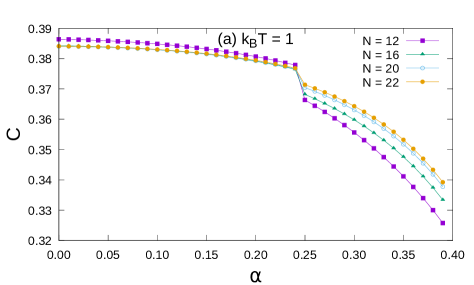
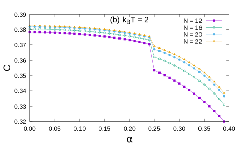
Figure 3: Nearest-neighbour concurrence of $J_{1}-J_{2}$ model for different system sizes at constant temperature. The connotations here are the same as in Fig. 2, but at a constant temperature with a varying mixing probability at each $\alpha$ for different system sizes. Here, in panel (a) $k_{B}T=1$, and in panel (b) $k_{B}T=2$ (in units of $J_{1}\hbar$). The quantity plotted along the horizontal axes are dimensionless and the same along the vertical axes are in ebits.

With increase in $p$, the jump increases and becomes more prominent. The point of discontinuity, which we consider to be the point of phase transition ($\alpha_{c}$) is the same for all values of $p$ for a fixed $N$. The neighbourhood, of the phase transition point is magnified and plotted in the insets of both the panels. The nature of concurrence is highly oscillating in this near-critical regime and the amplitude of oscillation increases with the increase of $p$ values. For determining the critical point, $\alpha_{c}$, we take the average of the two $\alpha$ values just before and just after the discontinuous jump in the concurrence. See the insets of Fig. 1.

In Fig. 2 we consider the same phenomenon but from a different perspective. Here we fix the values of $p$ of the subjacent state in each panel and investigate the nature of concurrence for different values of $N$. This time the figure reveals a different characteristic of the transition point. For a fixed $N$, the critical transition point ($\alpha_{c}$) is independent of $p$ (see Fig. 1), whereas $\alpha_{c}$ decreases as the system size $N$ increases, for a fixed value of $p$. A tabular representation as a proof of this fact is presented in Table 1.

Note that the discrete jump in nearest-neighbor concurrence only occurs when applying periodic boundary conditions. When we apply an open boundary condition to the same model described in Eq. (1), specifically by setting the range of the first summation in Eq. (1) to run from $i=1$ to $N-1$ and the range of the second summation to run from $i=1$ to $N-2$, we observe that the nearest-neighbour concurrence of the subjacent state monotonically increases for system sizes that are twice odd numbers (e.g., $N=10,14,18$), while it monotonically decreases for system sizes that are twice even numbers (e.g., $N=12,16,20$). We do not detect any discontinuity in the concurrence within the region of $J_{2}/J_{1}=\alpha\in[0.0,0.5]$ for these cases. This may be because of the finite size effects of the quantum chain with open boundaries.

$N$	$\alpha_{c}$	$N$	$\alpha_{c}$
8	0.24630	18	0.24221
10	0.24449	20	0.24201
12	0.24349	22	0.24180
14	0.24286	24	0.24164
16	0.24248

Table 1: The values of $\alpha_{c}$ for increasing size $(N)$ of the system for $p=0.30$ in the subjacent state for the $J_{1}-J_{2}$ model. All quantities are dimensionless.

This approach of utilising the subjacent state to detect the phase transition in the $J_{1}-J_{2}$ Heisenberg spin chain can be extended to the $J_{1}-J_{2}$ model on a two-dimensional lattice. The two-dimensional $J_{1}-J_{2}$ Heisenberg spin model is governed by the Hamiltonian,

$$H_{2-d}=J_{1}\hbar\sum\vec{\sigma}_{i}\cdot\vec{\sigma}_{j}+J_{2}\hbar\sum\vec{\sigma}_{i}\cdot\vec{\sigma}_{k}.$$ (4)

Here the first summation involves pairs of nearest neighbours, whereas the second summation deals with pairs of nearest neighbours along the diagonals. In Fig. 4, we plot the nearest-neighbour concurrence of this two-dimensional $J_{1}-J_{2}$ model, for $N=16$, on a $4\times 4$ lattice. Our findings reveal a discontinuous jump in the nearest-neighbour concurrence at approximately $\alpha\approx 0.4$, which indicates a phase transition from ‘ordinary-Néel order’ to an intermediate phase of a ‘plaquette or columnar dimer’ phase. It can be shown that the same methodology also detects the (anti-)ferromagnetic to paramagnetic phase transition in the one-dimensional transverse Ising model, where the concurrence attains a maximum at the critical point.

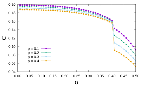
Figure 4: Nearest-neighbour concurrence of the two-dimensional $J_{1}-J_{2}$ model for $N=16$ on a $4\times 4$ lattice. Here we have depicted the nearest-neighbour concurrence with relative coupling strength $\alpha$, for different values of the mixing probability $p$ of the subjacent state. The quantity plotted along the horizontal axis is dimensionless and the same along the vertical axis is in ebits.

Till now, we were considering the situation where the mixing probability $p$ is left constant while nearest neighbour concurrence is investigated with varying relative coupling strengths, $\alpha$. See Figs.  1 and  2. This implies that we require the temperature to be changed at each $\alpha$ to keep the mixing probability fixed with the changes of $\alpha$. Arguably, a more practical study is to investigate the nature of nearest neighbour concurrence at a fixed temperature. Therein, the probability $p$, of the subjacent state, change with $\alpha$, as the change in $\alpha$ leads to changes in $E^{(1)}(N,\alpha)$ and $E^{(0)}(N,\alpha)$. For our analysis, we fixed the temperature to $k_{B}T=1\text{ and }2$. At very low temperatures, the system’s state would consist, for practical purposes, of a mixture of the ground state and the first-excited state. Essentially, the excited state serves as a source of thermal noise in the system. To model a situation where this thermal noise arises due to a non-zero temperature, we can envision the mixed state as being associated with a fixed temperature, or with a fixed admixture of the excited state. The former is considered in Figs. 1 and 2, while the latter is taken up in Fig. 3. We find that both these noise models lead to the same phase transition points for the parent Hamiltonian.

From Fig. 2, it is evident that by keeping the mixing probability ($p$) constant, we can observe the phase transition in the one-dimensional $J_{1}-J_{2}$ model as we vary $\alpha$. Since fixing the probability leads to temperature variations with changes in $\alpha$, this phase transition might be construed as being induced by temperature. However, as illustrated in Figs. 2 and 3, the nearest-neighbor concurrence at fixed temperature and at fixed $p$ is similar in nature, and the estimated critical point of phase transition is also at the same point in the parameter space in both the cases. In the case of phase transitions induced by thermal fluctuations, the phase transition becomes apparent as the system’s temperature varies. Given that the critical point remains constant in scenarios where the temperature is fixed, it follows that the observed phase transitions are not induced by thermal fluctuations. Therefore, we can infer that the phase transition we observe here is not thermally induced.

Further illustrations are done for fixed $p$. Investigations at fixed temperature will provide equivalent information. The difference between the values of concurrence $\Delta C$, just before and after the transition point, decreases as we increase the system size. The numerical values of $\Delta C$s for increasing system size, for a fixed $p$, are given in Table 2. This may potentially be a disadvantage in the thermodynamic limit, $N\rightarrow\infty$. A finite-size scaling is needed to see whether concurrence can still play the role of a good detector of phase transition in a mixture of ground and first excited state for $N\rightarrow\infty$.

$N$	$\Delta C$	$N$	$\Delta C$
8	$3.2\times 10^{-2}$	18	$6.8\times 10^{-3}$
10	$2.0\times 10^{-2}$	20	$5.6\times 10^{-3}$
12	$1.4\times 10^{-2}$	22	$4.8\times 10^{-3}$
14	$1.1\times 10^{-2}$	24	$4.2\times 10^{-3}$
16	$8.3\times 10^{-3}$

Table 2: The values of $\Delta C$ (in ebits) for different sizes ($N$) of the system for $p=0.30$, for the $J_{1}-J_{2}$ model.

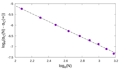
Figure 5: Critical point of the $J_{1}-J_{2}$ model in the thermodynamic limit for the subjacent state at $p=0.30$. Here we have fitted the values of $\alpha_{c}$ corresponding to different $N$ obtained from Table 1, with Eq. (5). The data points are shown by blue dots and the black dotted line represents the fitting curve. Both the axes are plotted in $\log$ scale and the quantities plotted are dimensionless.

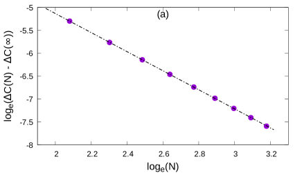
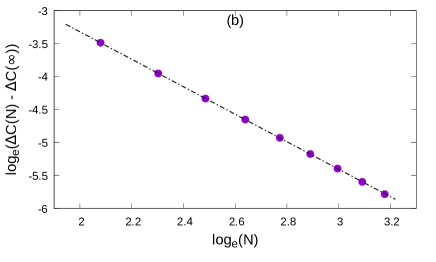
Figure 6: Jump in concurrence at critical point at thermodynamic limit. Here we have fitted the values of $\Delta C$ for different $N$ with Eq. (6) for (a) $p=0.05$ and (b) $p=0.30$. The data points are shown by blue dots and the black dotted line represents the fitting curve. The axes are plotted in $\log$ scale and the quantity described along vertical axes are in ebits whereas the same along horizontal axes is dimensionless.

As the precise quantum phase transition point on the $\alpha$-axis for an infinitely large system is unknown, we extrapolate the transition points of $N=8,10,12,14,16,18,20,22,24$ size systems to $N=\infty$. To extrapolate, we have chosen the fitting function, viz.

$$\alpha_{c}(N)=\alpha_{c}(\infty)+aN^{-b}.$$ (5)

On fitting the values of $\alpha_{c}(N)$ with the system size ($N$) from Table 1, we obtain $\alpha_{c}(\infty)=0.24099$ with the 95% confidence interval $\pm 4.9\times 10^{-9}$, $a=0.24$ (95% confidence interval $\pm 1.9\times 10^{-6}$) and $b=1.8$ (95% confidence interval $\pm 4.1\times 10^{-6}$). Thus the value of relative coupling ($\alpha$) at which there is a discontinuity, asymptotically tends to $\alpha_{c}=0.24099$, with the standard error $3.2\times 10^{-5}$, for $p=0.30$ in the subjacent state. Here we have used non-linear least-square fitting to find the values of the parameters, the $95\%$ confidence intervals, and the error, for the fitting curves [141, 142, 143]. We can also see from Fig. 5 that the difference, $\alpha_{c}(N)-\alpha_{c}(\infty)$, decreases almost linearly with the increase of $N$, when plotted in $\log-\log$ scale.

Having obtained the transition point (for $p=0.30$) in the thermodynamic limit, we can now investigate the utility of concurrence as a phase transition detector at $N\rightarrow\infty$.For checking this, we fit the values of $\Delta C$ for different $p$’s with the following expression:

$$\Delta C(N)=\Delta C(\infty)+\gamma N^{-\delta}.$$ (6)

We find that for $p=0.30$ as well as for other values of $p$, the jump does not asymptotically tend to zero. There is some finite discontinuity $\Delta C(\infty)$ as $N\rightarrow\infty$ and hence we have achieved our goal of finding a quantum information-theoretic indicator of phase transition in the thermodynamic limit. The numerical values of the jumps in the thermodynamic limit, $\Delta C(\infty)$, for different values of mixing probability, along with the standard errors of fitting, are given in Table 3. The scaling exponent $\delta$ in (6), turns out to be approximately 2.08 for all values of $p$.

$p$	$\Delta C(\infty)$	Error
0.01	$8.3\times 10^{-4}$	$2.9\times 10^{-7}$
0.05	$8.6\times 10^{-4}$	$4.1\times 10^{-6}$
0.10	$9.1\times 10^{-4}$	$9.1\times 10^{-6}$
0.15	$9.6\times 10^{-4}$	$1.5\times 10^{-5}$
0.20	$1.0\times 10^{-3}$	$1.7\times 10^{-5}$
0.25	$1.1\times 10^{-3}$	$2.5\times 10^{-5}$
0.30	$1.1\times 10^{-3}$	$1.8\times 10^{-5}$
1.00	$1.8\times 10^{-3}$	$8.4\times 10^{-5}$

Table 3: The asymptotic values of $\Delta C$ (in ebits) in the thermodynamic limit ($N\rightarrow\infty$) for different values of $p$, for the $J_{1}-J_{2}$ model.

The fitting functions and the corresponding $\Delta C(N)-\Delta C(\infty)$ (in $\log-\log$ scale) with respect to system size $N$ for two fixed values of $p$ is demonstrated in Fig. 6. We have performed the analysis also for other values of $p$ and found a qualitatively similar behaviour. The behaviour is very similar to that of $\alpha_{c}(N)-\alpha_{c}(\infty)$. Both decreases almost linearly with the increase of $N$ on the $\log-\log$ scale. Compare Figs. 5 and 6.

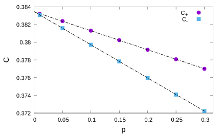
Figure 7: Nearest neighbour concurrence just before and just after the jump near the critical point of the $J_{1}-J_{2}$ model for the subjacent state. Here we have looked into the dependence of $C_{+}$ and $C_{-}$ on $p$ for $N=20$. The rectangular dots are the values before the discontinuity ($C_{-}$) and the circular dots are the same just after the jump ($C_{+}$). The dotted lines represent the corresponding fitting functions. The quantity plotted along the horizontal axis is dimensionless and the same described along the vertical axis is in ebits.

Till now we were discussing about the phase transition point of the $J_{1}-J_{2}$ model, and the jump in concurrence at that point. It could also be interesting to study the values of nearest neighbour concurrence in the vicinity of phase transition point and its dependence on the mixing probability $p$ for different system sizes. We depict the dependence of concurrence, just before the jump by $C_{-}$ and the same just after the jump by $C_{+}$, on $p$ for $N=20$ in Fig. 7, with rectangular and circular dots respectively. We find that for small values of $p$, the values of concurrence, either way about the point of discontinuity, decreases linearly. The behaviour is similar for other values of $N$ too. Here we end our discussion about the phase transition of the ideal $J_{1}-J_{2}$ Heisenberg spin chain. In the succeeding sections, we will look into the response to anisotropy and disorder of the phase diagram of the model.

IV Response to anisotropy of the phase transition point

The one-dimensional $J_{1}-J_{2}$ Heisenberg spin model with an anisotropic coupling constant along $z$-direction can be named as the one-dimensional spin-$\frac{1}{2}$ $XXZ$ $J_{1}-J_{2}$ spin model and its governing Hamiltonian may be written as

$$H_{XXZ}=J_{1}\hbar\sum_{i=1}^{N}(\vec{\sigma}_{i}\cdot\vec{\sigma}_{i+1})_{\delta}+J_{2}\hbar\sum_{i=1}^{N}(\vec{\sigma}_{i}\cdot\vec{\sigma}_{i+2})_{\delta},$$ (7)

where $(\overrightarrow{\sigma_{i}}\cdot\overrightarrow{\sigma_{j}})_{\delta}=\sigma_{i}^{x}\sigma_{j}^{x}+\sigma_{i}^{y}\sigma_{j}^{y}+\delta\sigma_{i}^{z}\sigma_{j}^{z}$ with $\delta$ being a dimensionless anisotropy constant. This model is known to have various quantum phases [79] and can describe the spin-Peierls compound CuGeO₃ [144, 145]. As already discussed, the system is in a spin fluid state for $\alpha\lesssim 0.24$ and $\delta<1$, and it goes to a Néel phase for $\delta>1$. For $\alpha\gtrsim 0.24$, the system goes into a dimer phase. A schematic representation of these phase boundaries is shown in the left panel of Fig. 8.

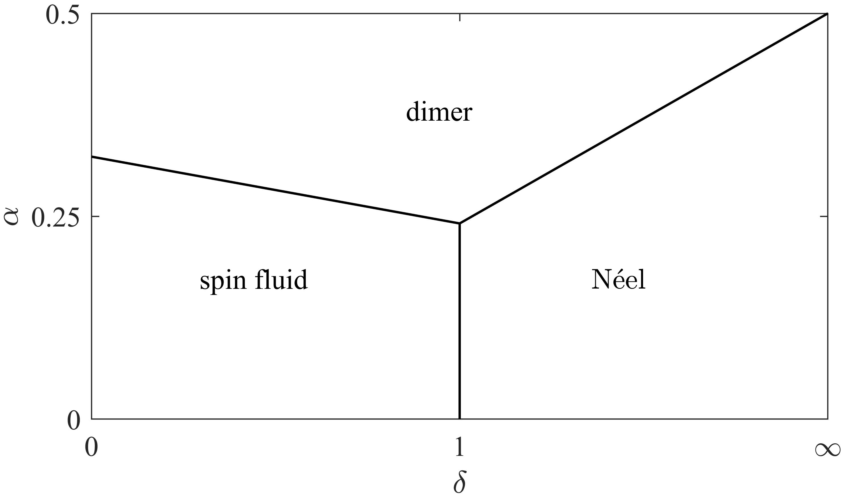
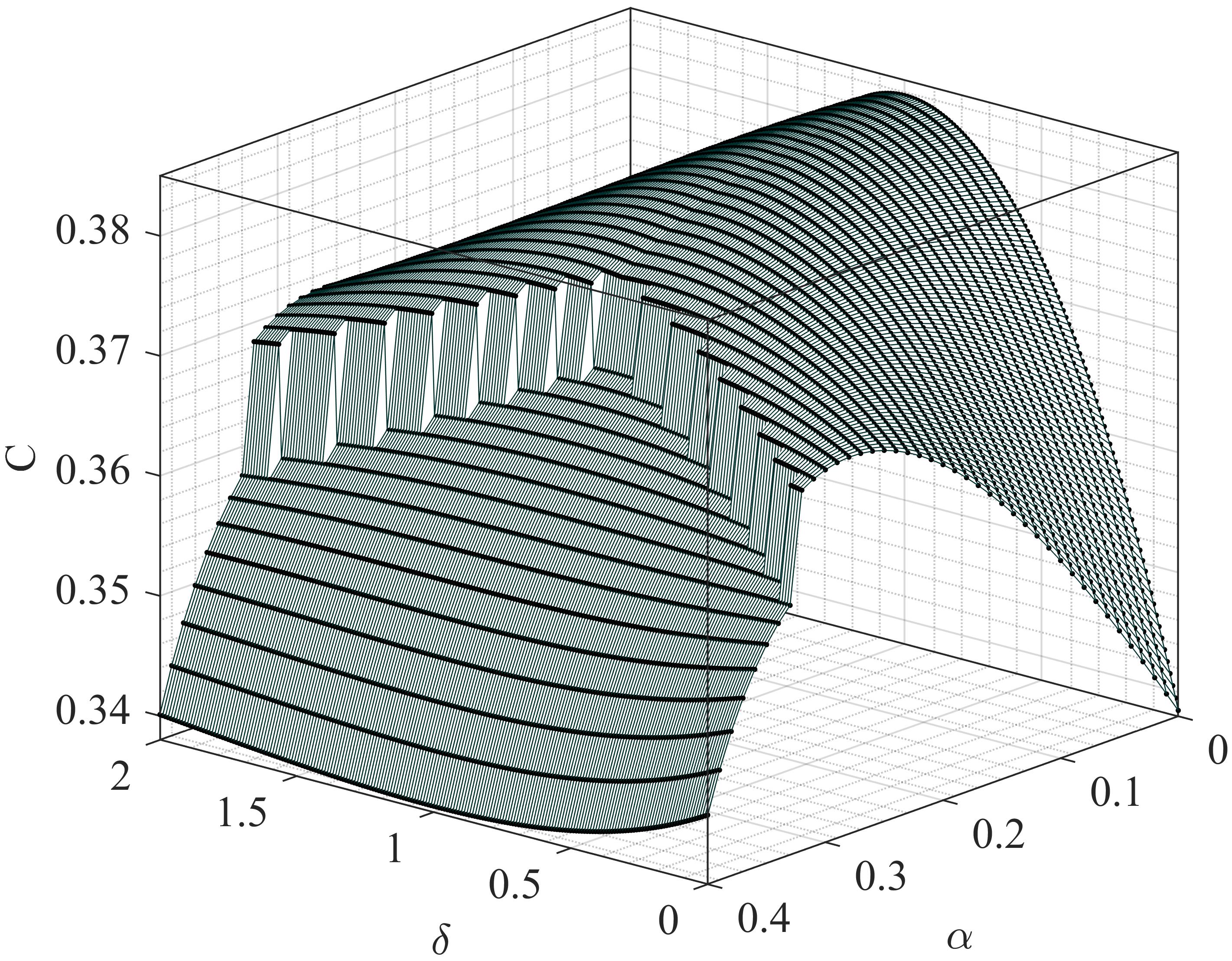
Figure 8: Phase diagram of the XXZ $J_{1}-J_{2}$ spin model. The left panel represents a schematic quantum phase diagram of the one-dimensional XXZ $J_{1}-J_{2}$ spin model on the $(\alpha$ , $\delta)$ plane. In the right panel, we have plotted the nearest neighbour concurrence of the subjacent state on the $(\alpha,\delta)$ plane, and considered it as an order parameter for the transitions in the XXZ $J_{1}-J_{2}$ model. Here, $N=16$. The concurrence $(C)$ is in ebits, while all other quantities are dimensionless.

In the previous section, we have studied the behaviour of concurrence by changing the mixing probability. In this section, we have taken a fixed mixing probability $p$. All further analysis is done for

$$p=0.2689\approx\frac{e^{-1}}{1+e^{-1}}.$$ (8)

We are therefore fixing the temperature as $T\approx\frac{E^{(1)}(N,\alpha)-E^{(0)}(N,\alpha)}{k_{B}}$ for each $\alpha$. Now we investigate the behaviour of concurrence on the $(\alpha,\delta)$ parameter space. In the right panel of Fig. 8, we observe that there is a dip in the concurrence along the $\delta=1$ line for low $\alpha$, indicating the spin fluid to Néel order quantum phase transition. It shows a sharp drop to indicate the spin fluid to dimer quantum phase transition for $\delta<1$, and a sharp jump to indicate the dimer to Néel quantum phase transition for $\delta>1$. Thus, we observe that a discontinuity in the concurrence serves as an indicator of a phase transition between the spin fluid and dimer phases in the anisotropic one-dimensional $J_{1}-J_{2}$ model. Also, the phase transition between Néel and dimer is also signified by discontinuity of concurrence. On the other hand, we observe that the phase transition between the spin-fluid and Néel phases is distinguished by a discontinuity in the first derivative of the concurrence. So, here the nature of the signatures observed in concurrence varies for different phase transitions. In this regard, it is important to note that, as the discontinuity in the order parameter is indicative of a phase transition, it is also quite common for order parameters to display continuity near the critical point, while their derivatives exhibit discontinuities, as observed in [146, 147]. The points of transition, say along lines parallel to the $\alpha$-axis, are calculated by using exact diagonalisation on finite systems. A finite-size scaling analysis is therefore useful. For a fixed $\delta$, we fixed the critical point $\alpha_{C}(\delta,N)$, for a system of size $N$, and use the rational polynomial,

$$f\left(N\right)=\frac{p_{1}N^{2}+p_{2}N+p_{3}}{N^{2}+q_{1}N+q_{2}},$$ (9)

to estimate the quantum phase transition point of an infinitely large system  [148]. The corresponding phase diagram, using both finite-size predictions as well as the extrapolated ones is presented in the upper left panel of Fig. 9. We analyse their finite-size scaling behavior, by fitting a function of the form,

$${\color[rgb]{0,0,0}\alpha_{c}(N)=\alpha_{c}(\infty)+a^{\prime}N^{-\beta}},$$ (10)

and obtain the finite size scaling exponents $(\beta)$ for different $(\delta)$. The corresponding data for $\delta<1$ is presented in  A I and the same for $\delta\geq 1$ is shown in  A II, in the Appendix A. Here $\alpha_{c}(\infty)$ is the value of $\alpha_{c}$ for $N\rightarrow\infty$ and $a^{\prime}$ is a constant. We magnify the region around the multi-criticality point for $\alpha\approx 0.24$ and $\delta=1$, in the inset of of the upper left panel of Fig. 9.

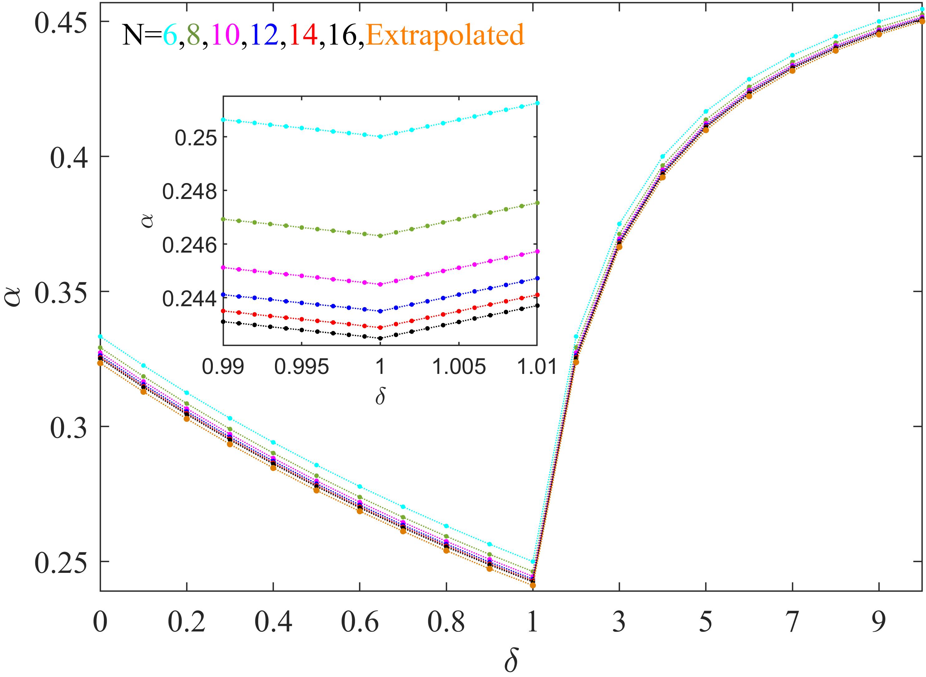
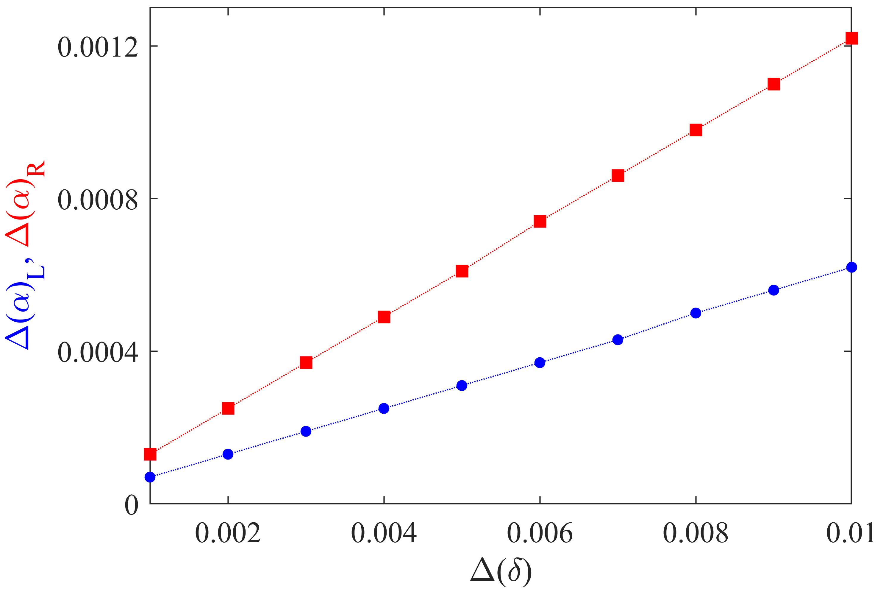
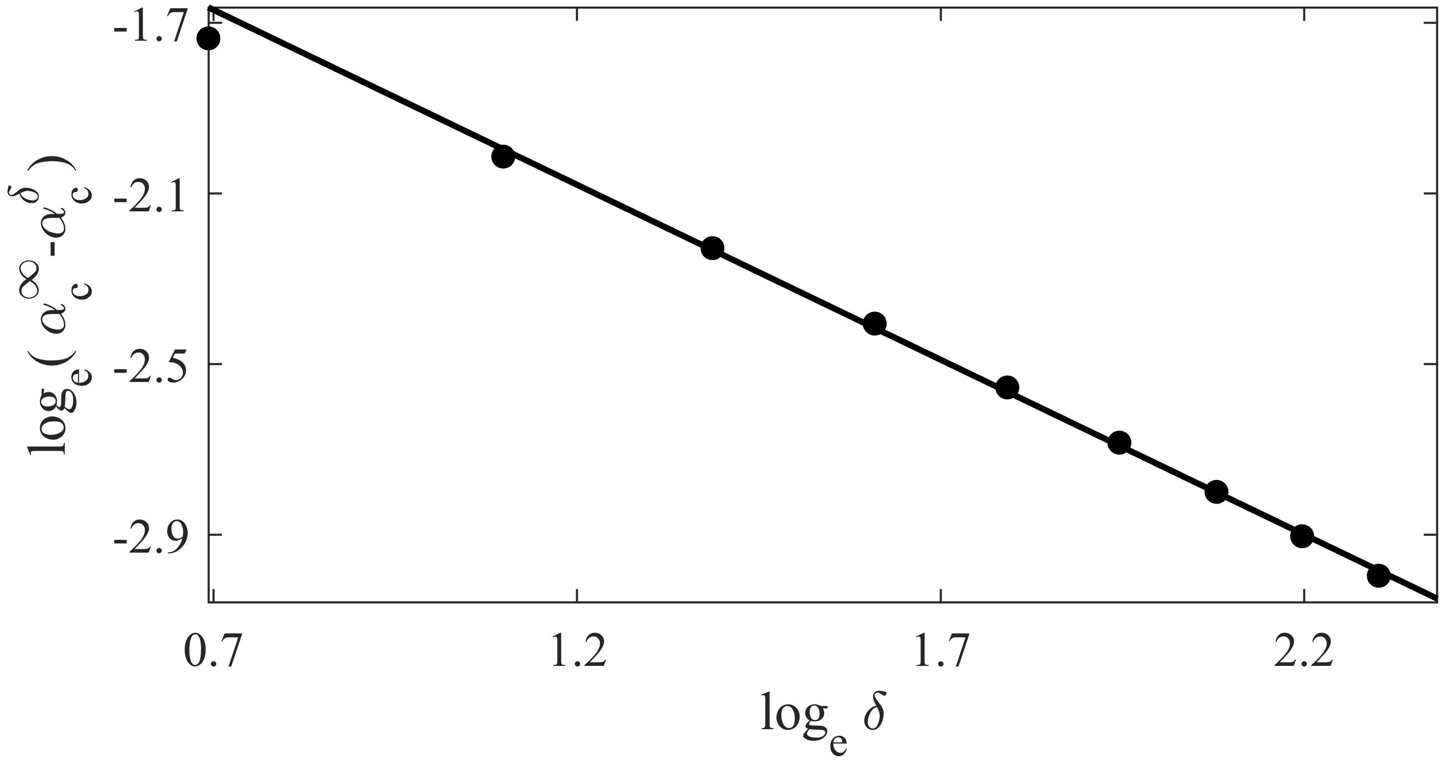
Figure 9: Phase diagram and finite-size scaling for transitions of the XXZ $J_{1}-J_{2}$ model. The phase diagram is presented in the upper left panel. We focus on the transitions to the dimer phase and the multi-critical point. The transitions are assumed to be signaled by the discontinuities of the nearest neighbour concurrence in the subjacent state. The orange dots correspond to the extrapolated discontinuity points in the large $N$ limit. A magnified version of this depiction closer to the $\delta=1$ region is shown in the inset. In the upper right panel, we compare the nature of critical transition points on the two sides of $\delta=1$. Here we take the magnitude of the distance from $\delta=1$ as $\Delta(\delta)$ and depict the corresponding $\alpha_{c}$ values for both sides of the $\delta=1$ point. The critical $\alpha_{c}$ values on the left of $\delta=1$ is depicted by blue dots and the same on the right side are depicted by red squares for system size $N=16$. In the lower panel, we present the finite size scaling of the extrapolated critical transition points $\alpha_{c}$ along $\delta$-axis for $\delta>1$ for $N\rightarrow\infty$. For the values of scaling exponent and the corresponding $95\%$ confidence interval see the main text. All the quantities plotted along the axes in all the three panels are dimensionless.

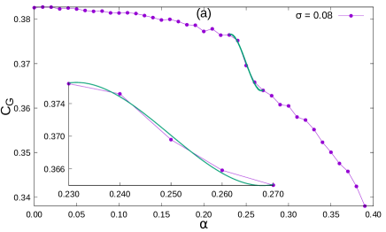
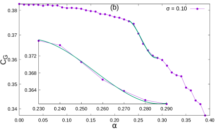
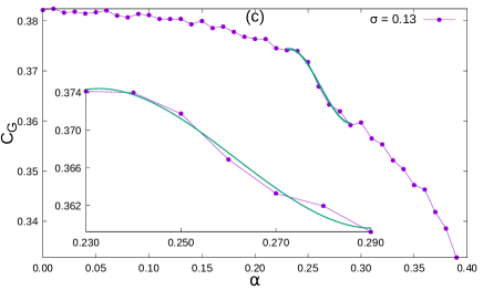
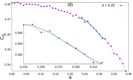
Figure 10: Nearest neighbour concurrence in presence of Gaussian disorder for $N=14$. The disorder averaged concurrence (averaged over $5\times 10^{4}$ realizations) is plotted along the vertical axes when the $\Delta$s are chosen independently from a Gaussian distribution with mean zero and for different values of the standard deviation $\sigma$ (given in the legends). The region close to the transition point is shown in the insets where the continuous line represents the polynomial fitting function. The quantity plotted along horizontal axes is dimensionless, whereas that plotted along vertical axes is in ebits.

We notice that the phase boundary changes with the change in $\delta$. The numerical values of critical phase transition points $\alpha_{c}$ decrease monotonically with the increase of $\delta$ from 0 to 1 and increase monotonically thereafter.

For further analysis, we plot the critical transition points $\alpha_{c}$ with respect to the distance in $\delta$ axis from the point $\delta=1$ in the upper right panel of Fig. 9, for $N=16$. From the inset of the upper left panel of Fig. 9, we can observe an asymmetry in $\alpha_{c}$ values on the two sides of $\delta=1$. This asymmetry is clearer in the upper right panel. We can see that the slope of the curves representing the $\Delta\alpha$ values for the $\delta>1$ region is much greater than those for the $\delta<1$ one.

We find that $\alpha_{c}$ approaches $\frac{1}{2}$ in the limit of $\delta\rightarrow\infty$. We now analyse the scaling behavior of the phase transition point with $\delta$. We choose the fitting function,

$$\alpha_{c}^{\delta}=\alpha_{c}^{\infty}-a^{\prime\prime}\delta^{-d},$$ (11)

where $\alpha_{c}^{\infty}$ is the value of $\alpha_{c}$ at $\delta=\infty$ and $a^{\prime\prime}$ is a constant. We present the variation of $\alpha_{c}^{\infty}-\alpha_{c}^{\delta}$ against $\delta$ (both on $\log$ scale) for $N\rightarrow\infty$ in the lower panel of Fig. 9. The scaling exponent is found to be $d=0.82$ with 95% confidence interval $\pm 0.025$ and the standard error is $0.012$

V Response to glassy disorder of the phase transition point

A system is said to be glassy disordered if there is a disordered system parameter whose equilibration time is much larger than the time spans relevant for our investigations of the system. So, during the time of observation, the disordered parameters effectively do not change for a certain realization of disorder. This disorder is analogous to that of a spin glass system [89, 149, 150]. Glassy disorder has also been referred to as a quenched disorder [1, 89, 149, 150, 151, 152, 153]. Studies on spin chains with glassy disorder include [83, 87, 88, 108, 117, 121, 154, 155, 156, 127, 123, 124, 126, 129]. Here we study the effect of introduction of a glassy disorder parameter in the $J_{1}-J_{2}$ model. We analyse the response of the quantum phase transition point on introduction of a glassy anisotropy parameter. Precisely, we insert a $z-z$ interaction term in the $J_{1}-J_{2}$ Hamiltonian  (1) for each Heisenberg interaction term $\vec{\sigma}_{i}\cdot\vec{\sigma}_{j}$. The unit-free coupling strength, $\Delta$, for each interaction then is independently distributed with respect to that for any other term. However, they are all Gaussian distributed with vanishing mean and standard deviation $\sigma$:

$$P(\Delta)=\frac{1}{\sigma\sqrt{2\pi}}e^{-\frac{1}{2}\big{(}\frac{\Delta}{\sigma}\big{)}^{2}},\quad-\infty<\Delta<\infty.$$ (12)

The considerations in this section are therefore complementary to those in the preceding one, even though both deal with a z-z interaction anisotropy in the $J_{1}-J_{2}$ model. Note that the usual $J_{1}-J_{2}$ model lies in the $\sigma\rightarrow 0$ limit for the analysis of the glassy disordered model of this section. In comparison, the same limit is obtained for $\delta\rightarrow 1$ for the considerations of the XXZ $J_{1}-J_{2}$ model of the preceding section. The disorder averaged concurrence is given by

$$C_{G}=\int_{-\infty}^{\infty}C(\tilde{\Delta})\frac{1}{\sigma\sqrt{2\pi}}e^{-\frac{1}{2}\big{(}\frac{\tilde{\Delta}}{\sigma}\big{)}^{2}}d\tilde{\Delta}.$$ (13)

Here, $\tilde{\Delta}$ represents the entire collection of $\Delta$s of the system, and the $\tilde{\Delta}^{2}$ in the exponent denotes the sum of the square of such $\Delta$s. We use Monte Carlo integration to evaluate the integral. Now for each realisation, $\Delta$s are chosen independently by choosing random numbers from a Gaussian distribution with mean zero and standard deviation $\sigma$, and then the nearest neighbour concurrence is calculated for that realisation by using the subjacent state. We average over a large number of realisation and check for convergence.

In presence of the glassy disorder in the parameter $\Delta$, the concurrence shows a behaviour similar to that of the ordered case and a sufficiently visible difference in the values of concurrence before and after the phase transition point is observed. See Fig. 10 in this regard. The difference is that the change in concurrence around the phase transition point is not as sharp as that in the ideal situation. The discontinuity in concurrence at the phase transition point becomes less and less prominent, as we increase the strength of disorder, ie., the standard deviation $\sigma$ of the disorder distribution. As we increase $\sigma$ to more than $0.2$, it becomes difficult to point out the region around the phase transition point.

Since the discontinuity in the profile of the concurrence is not sharp, we adopt here a method that is different from the one used until now to identify the phase transition. As we see from Fig. 10, the profile of concurrence with $\alpha$ goes from concave to convex at the phase transition point. We can then fit a cubic polynomial in the near-critical region, and the inflection point of the polynomial can be considered as the point of phase transition. The inflection point of a cubic polynomial is the point where the function changes its curvature from negative to positive or vice versa, and hence the polynomial has a vanishing double derivative at this point. Suppose that the cubic polynomial is given by

$$C_{G}(\alpha)=a_{1}\alpha^{3}+b_{1}\alpha^{2}+c_{1}\alpha+d_{1}.$$ (14)

The near-critical region along with the fitting function are shown in the insets of Fig. 10. The values of the critical points for different system sizes by changing the strength of disorder are given in Table A III for the mixing probability $p=0.2689$ (see (8)), and in Table A IV for mixing probability $p=0.1344$, along with the standard errors of fitting. The phase transition point gradually shifts to higher $\alpha$ with the increase of the strength of disorder ($\sigma$). Furthermore, we analyse the finite-size scaling for the case of $p=0.2689$ from the data set in Table A III. The fitting function is of the form,

$$\alpha_{C}^{\text{dis}}(N)=\alpha_{C}^{\text{dis}}(\infty)+aN^{-b}.$$

For $\sigma=0.05$, $\alpha_{C}^{\text{dis}}(\infty)=0.2476$ and $b=7.69$ and for $\sigma=0.08$, $\alpha_{C}^{\text{dis}}(\infty)=0.2492$ and $b=7.38$. For the former, the root-mean-square error of the fitting function is $0.87\times 10^{-3}$, and for the latter, the same is $0.94\times 10^{-3}$.

Throughout this study, we have utilised the subjacent state to detect the phase transition of a $J_{1}-J_{2}$ Heisenberg spin chain. However, it is important to ask, if any mixed state other than the subjacent state, defined in Eq. (3), can show signatures of phase transition. In the work presented in [78], it was demonstrated that, for the one-dimensional $J_{1}-J_{2}$ model, the thermal state, i.e., the canonical equilibrium state, which is a mixture of all possible energy eigenstates, exhibits no discontinuity in nearest neighbor concurrence near the critical point. Furthermore, the authors explored a scenario where the full multiplet was not included, and the mixture incorporated states up to the third excited state. In this particular case as well, they did not observe any discontinuity in the nearest neighbor concurrence near the critical point. Therefore, it becomes evident that employing the subjacent state is more advantageous in detecting quantum phase transitions in a $J_{1}-J_{2}$ Heisenberg spin chain compared to using the thermal state or states composed of higher energy levels.

VI Conclusion

We have investigated the utility of nearest neighbour entanglement of a mixture of the ground and first excited states - the subjacent states - which mimic the low but non-zero temperature states of the system, for detection and analysis of quantum phase transitions in one-dimensional $J_{1}-J_{2}$ Heisenberg quantum spin models. We want to find signatures of the ground state quantum phase transitions in a given physical system at low but finite temperatures by utilizing the subjacent states. This is of significant interest because a real physical system will always be at a finite temperature. We try to find the extent to which such a finite-temperature state can mirror the zero-temperature transitions in the system. We have studied the dependencies of the critical phase transition point on the mixing probability, and found that concurrence - a measure of two-qubit entanglement - can play the role of a good order parameter even if the ground state probability is large compared to that of the first excited state, whereas it is already known that the ground state concurrence itself cannot perform the role of a good indicator of phase transition in these models. We have extrapolated the results to the thermodynamic limit and obtained the phase transition point $\alpha_{c}\approx 0.24099$, for the isotropic $J_{1}-J_{2}$ Heisenberg quantum spin chain with $\alpha=J_{2}/J_{1}$, which is very close to the value already known in literature, obtained by various methods [68, 70, 74, 75] and we have also shown that the critical point does not depend on this mixing probability.

Moreover, we applied the same order parameter of the subjacent state for analysing phase transitions in the $J_{1}-J_{2}$ model, tweaked by either anisotropy or glassy disorder in the coupling strengths. We introduced anisotropy in one specific direction for both the nearest neighbour and next-nearest neighbour interactions, and studied the effect of anisotropy on the critical phase transition point for various system sizes, and subsequently extrapolated to the thermodynamic limit. Here, we obtained a phase diagram of the anisotropic $J_{1}-J_{2}$ model, which shows the phase boundaries of the existent phases of the system like spin fluid state, dimer phase and Néel phase. In previous works, these phase boundaries of an anisotropic $J_{1}-J_{2}$ model was detected by some other order parameters  [79, 80], but we showed that detection of such phase boundaries is possible at finite temperature with a quantum-informatics order parameter.

Separately, we incorporated a glassy disorder parameter in a coupling of the $J_{1}-J_{2}$ model and investigated its effect on the phase diagram. We observed that the disorder smoothens the marker of phase transition. The phase transition point also shifted towards higher values of $\alpha$ depending on the strength of the disorder. Importantly, we performed finite-size scaling in each of the cases considered. The phenomenon of phase transition of a disordered $J_{1}-J_{2}$ model is already studied in the literature, but having the nearest neighbour entanglement as an indicator of phase transition, even in presence of disorder in this model, is a potentially interesting result, which reveals the usefulness of quantum information theoretic properties in detecting paradigmatic many-body phenomena in a realistic scenario. We believe that the results would lead towards the establishment of the consideration of physical quantities in the subjacent state as a proper and fruitful order parameter for detection and characterisation of cooperative physical phenomena, since such quantities in the subjacent state are theoretically accessible just like ground state physical quantities and experimentally more viable in comparison to the same.

VII Acknowledgement

We acknowledge computations performed using Armadillo [157, 158] on the cluster computing facility of the Harish-Chandra Research Institute, India. This research was supported in part by the ‘INFOSYS scholarship for senior students’. We also acknowledge partial support from the Department of Science and Technology, Government of India through the QuEST grant (grant number DST/ICPS/QUST/Theme-3/2019/120).

Appendix A Tables

$\delta$	0	0.1	0.2	0.3	0.4	0.5	0.6	0.7	0.8	0.9
N = 6	0.33334	0.32259	0.31250	0.30304	0.29412	0.28572	0.27778	0.27028	0.26316	0.25642
N = 8	0.32924	0.31856	0.30851	0.29906	0.29017	0.28178	0.27387	0.26640	0.25934	0.25265
N = 10	0.32736	0.31668	0.30663	0.29717	0.28828	0.27989	0.27199	0.26453	0.25749	0.25082
N = 12	0.32628	0.31560	0.30556	0.29611	0.28722	0.27884	0.27094	0.26349	0.25646	0.24980
N = 14	0.32562	0.31494	0.30490	0.29546	0.28657	0.2782	0.27031	0.26286	0.25583	0.24918
N = 16	0.32518	0.31450	0.30447	0.29503	0.28614	0.27778	0.26989	0.26245	0.25542	0.24877
N $\approx$ $\infty$	0.32347	0.31286	0.30284	0.29342	0.28464	0.27632	0.26862	0.26120	0.25404	0.24732
$\beta$	1.80	1.82	1.82	1.83	1.88	1.90	2.00	2.01	1.92	1.88

Table A I: Critical transition points $\alpha_{c}$ for different values of $N$ along with the extrapolated $N\rightarrow\infty$ limit for $\delta<1$ using nearest neighbour concurrence of the subjacent state as the order parameter in the XXZ $J_{1}-J_{2}$ model. The last row presents the finite-size scaling exponents at different $\delta$.

$\delta$	1	2	3	4	5	6	7	8	9	10
N = 6	0.25000	0.33334	0.37500	0.40000	0.41667	0.42858	0.4375	0.44445	0.45000	0.45455
N = 8	0.24630	0.32928	0.37127	0.39664	0.41363	0.42581	0.43497	0.44212	0.44784	0.45253
N = 10	0.24449	0.32739	0.36956	0.39512	0.41228	0.4246	0.43388	0.44111	0.44692	0.45168
N = 12	0.24349	0.32634	0.36861	0.39428	0.41152	0.42392	0.43325	0.44054	0.44639	0.45120
N = 14	0.24288	0.32570	0.36803	0.39376	0.41106	0.42350	0.43288	0.44020	0.44608	0.45090
N = 16	0.24248	0.32528	0.36766	0.39342	0.41076	0.42323	0.43263	0.43997	0.44587	0.45071
N $\approx$ $\infty$	0.24116	0.32382	0.36647	0.39226	0.40973	0.42228	0.43172	0.43916	0.44517	0.45002
$\beta$	1.96	1.91	2.00	1.93	1.95	1.93	1.89	1.92	1.97	1.92

Table A II: Critical transition points $\alpha_{c}$ for different values of $N$ along with the extrapolated $N\rightarrow\infty$ limit for $\delta\geq 1$ using nearest neighbour concurrence of the subjacent state as the order parameter in the XXZ $J_{1}-J_{2}$ model. The last row presents the finite size scaling exponents at different $\delta$.

$\sigma$	$N=6$		$N=8$		$N=10$		$N=12$		$N=14$
	$\alpha_{C}$	error	$\alpha_{C}$	error	$\alpha_{C}$	error	$\alpha_{C}$	error	$\alpha_{C}$	error
0.05	$0.25434$	$0.0081$	$0.24881$	$0.0044$	$0.24608$	$0.0036$	$0.24820$	$0.0028$	$0.24834$	$0.0023$
0.08	$0.25521$	$0.0068$	$0.25038$	$0.00085$	$0.24750$	$0.0024$	$0.25002$	$0.0013$	$0.24968$	$0.00074$
0.10	$0.25567$	$0.0061$	$0.25154$	$0.0011$	$0.25415$	$0.0020$	$0.25416$	$0.0013$	$0.25629$	$0.00057$
0.13	$0.25975$	$0.0030$	$0.25804$	$0.0010$	$0.25761$	$0.00053$	$0.26736$	$0.00096$	$0.25547$	$0.00085$
0.15	$0.26095$	$0.0026$	$0.26053$	$0.00045$	$0.26215$	$0.0012$	$0.25951$	$0.00075$	$0.27500$	$0.00078$
0.18	$0.26237$	$0.0019$	$0.26618$	$0.00079$	$0.26659$	$0.00057$	$0.27478$	$0.00078$	$0.23801$	$0.00065$
0.20	$0.26442$	$0.0018$	$0.26821$	$0.00085$	$0.27002$	$0.00089$	$0.27985$	$0.00078$	$0.27977$	$0.00042$

Table A III: The values of $\alpha_{c}$ for different sizes of the system (N) and different $\sigma$ for the mixing probability $p=0.2689$, in the $J_{1}-J_{2}$ Heisenberg chain with glassy anisotropy.

$\sigma$	$N=6$		$N=8$		$N=10$		$N=12$		$N=14$
	$\alpha_{C}$	error	$\alpha_{C}$	error	$\alpha_{C}$	error	$\alpha_{C}$	error	$\alpha_{C}$	error
0.05	$0.25201$	$0.0046$	$0.24879$	$0.0020$	$0.24799$	$0.0016$	$0.24826$	$0.0015$	$0.24465$	$0.0014$
0.08	$0.25353$	$0.0043$	$0.25034$	$0.00071$	$0.25225$	$0.0012$	$0.25044$	$0.000033$	$0.25357$	$0.00078$
0.10	$0.25567$	$0.0031$	$0.25201$	$0.0000014$	$0.25557$	$0.00099$	$0.25363$	$0.00048$	$0.26879$	$0.00081$
0.13	$0.25860$	$0.0055$	$0.25701$	$0.0024$	$0.25590$	$0.0012$	$0.25849$	$0.00081$	$0.26155$	$0.00092$
0.15	$0.25943$	$0.0044$	$0.25749$	$0.0023$	$0.25878$	$0.0010$	$0.26269$	$0.00070$	$0.26787$	$0.00094$
0.18	$0.26058$	$0.0034$	$0.26094$	$0.0011$	$0.26262$	$0.0011$	$0.26387$	$0.00082$	$0.27721$	$0.00098$
0.20	$0.26540$	$0.0037$	$0.26238$	$0.00095$	$0.26604$	$0.00062$	$0.26943$	$0.00064$	$0.28565$	$0.00079$

Table A IV: The values of $\alpha_{c}$ for different sizes of the system (N) and different $\sigma$ for the mixing probability $p=0.1344$, in the $J_{1}-J_{2}$ Heisenberg chain with glassy anisotropy.

References

- Sachdev [2011] S. Sachdev, Quantum Phase Transitions, 2nd ed. (Cambridge University Press, Cambridge, 2011).
- Lewenstein et al. [2007] M. Lewenstein, A. Sanpera, V. Ahufinger, B. Damski, A. Sen(De), and U. Sen, Ultracold atomic gases in optical lattices: mimicking condensed matter physics and beyond, Advances in Physics 56, 243 (2007).
- Amico et al. [2008] L. Amico, R. Fazio, A. Osterloh, and V. Vedral, Entanglement in many-body systems, Rev. Mod. Phys. 80, 517 (2008).
- Carr [2011] L. D. Carr, Understanding Quantum Phase Transitions (CRC Press, Boca Raton, USA, 2011).
- Lewenstein et al. [2012] M. Lewenstein, A. Sanpera, and V. Ahufinger, Ultracold Atoms in Optical Lattices: Simulating quantum many-body systems (Oxford University Press, Oxford, 2012).
- Osborne and Nielsen [2002] T. J. Osborne and M. A. Nielsen, Entanglement in a simple quantum phase transition, Phys. Rev. A 66, 032110 (2002).
- Osterloh et al. [2002] A. Osterloh, L. Amico, G. Falci, and R. Fazio, Scaling of entanglement close to a quantum phase transition, Nature 416, 608 (2002).
- Horodecki et al. [2009] R. Horodecki, P. Horodecki, M. Horodecki, and K. Horodecki, Quantum entanglement, Rev. Mod. Phys. 81, 865 (2009).
- Gühne and Tóth [2009] O. Gühne and G. Tóth, Entanglement detection, Physics Reports 474, 1 (2009).
- Das et al. [2016a] S. Das, T. Chanda, M. Lewenstein, A. Sanpera, A. Sen De, and U. Sen, The separability versus entanglement problem, in Quantum Information: From Foundations to Quantum Technology Applications (John Wiley & Sons, Ltd, 2016) Chap. 8, pp. 127–174.
- Shimony [1995] A. Shimony, Degree of entanglement, Annals of the New York Academy of Sciences 755, 675 (1995).
- Barnum and Linden [2001] H. Barnum and N. Linden, Monotones and invariants for multi-particle quantum states, Journal of Physics A: Mathematical and General 34, 6787 (2001).
- Blasone et al. [2008] M. Blasone, F. Dell’Anno, S. De Siena, and F. Illuminati, Hierarchies of geometric entanglement, Phys. Rev. A 77, 062304 (2008).
- Das et al. [2016b] T. Das, S. S. Roy, S. Bagchi, A. Misra, A. Sen(De), and U. Sen, Generalized geometric measure of entanglement for multiparty mixed states, Phys. Rev. A 94, 022336 (2016b).
- Sen [De] A. Sen(De) and U. Sen, Bound genuine multisite entanglement: Detector of gapless-gapped quantum transitions in frustrated systems, arXiv:1002.1253 (2010a).
- Henderson and Vedral [2001] L. Henderson and V. Vedral, Classical, quantum and total correlations, Journal of Physics A: Mathematical and General 34, 6899 (2001).
- Ollivier and Zurek [2001] H. Ollivier and W. H. Zurek, Quantum discord: A measure of the quantumness of correlations, Phys. Rev. Lett. 88, 017901 (2001).
- [18] P. Štelmachovič and V. Bužek, Quantum information approach to the ising model, arXiv:quant-ph/0312154 .
- Lambert et al. [2005] N. Lambert, C. Emary, and T. Brandes, Entanglement and entropy in a spin-boson quantum phase transition, Phys. Rev. A 71, 053804 (2005).
- Roscilde et al. [2005] T. Roscilde, P. Verrucchi, A. Fubini, S. Haas, and V. Tognetti, Entanglement and factorized ground states in two-dimensional quantum antiferromagnets, Phys. Rev. Lett. 94, 147208 (2005).
- Bose and Tribedi [2005] I. Bose and A. Tribedi, Thermal entanglement properties of small spin clusters, Phys. Rev. A 72, 022314 (2005).
- Bužek et al. [2005] V. Bužek, M. Orszag, and M. Roško, Instability and entanglement of the ground state of the dicke model, Phys. Rev. Lett. 94, 163601 (2005).
- Anfossi et al. [2005] A. Anfossi, P. Giorda, A. Montorsi, and F. Traversa, Two-point versus multipartite entanglement in quantum phase transitions, Phys. Rev. Lett. 95, 056402 (2005).
- de Oliveira et al. [2006a] T. R. de Oliveira, G. Rigolin, and M. C. de Oliveira, Genuine multipartite entanglement in quantum phase transitions, Phys. Rev. A 73, 010305 (2006a).
- Cavalcanti et al. [2006] D. Cavalcanti, F. G. S. L. Brãndao, and M. O. T. Cunha, Entanglement quantifiers, entanglement crossover and phase transitions, New Journal of Physics 8, 260 (2006).
- Rigolin et al. [2006] G. Rigolin, T. R. de Oliveira, and M. C. de Oliveira, Operational classification and quantification of multipartite entangled states, Phys. Rev. A 74, 022314 (2006).
- de Oliveira et al. [2006b] T. R. de Oliveira, G. Rigolin, M. C. de Oliveira, and E. Miranda, Multipartite entanglement signature of quantum phase transitions, Phys. Rev. Lett. 97, 170401 (2006b).
- Anfossi et al. [2007] A. Anfossi, P. Giorda, and A. Montorsi, Entanglement in extended hubbard models and quantum phase transitions, Phys. Rev. B 75, 165106 (2007).
- Costantini et al. [2007] G. Costantini, P. Facchi, G. Florio, and S. Pascazio, Multipartite entanglement characterization of a quantum phase transition, Journal of Physics A: Mathematical and Theoretical 40, 8009 (2007).
- Dahlsten et al. [2007] O. C. O. Dahlsten, R. Oliveira, and M. B. Plenio, The emergence of typical entanglement in two-party random processes, Journal of Physics A: Mathematical and Theoretical 40, 8081 (2007).
- Sen [De] A. Sen(De) and U. Sen, Channel capacities versus entanglement measures in multiparty quantum states, Phys. Rev. A 81, 012308 (2010b).
- [32] M. N. Bera, R. Prabhu, A. Sen(De), and U. Sen, Multisite entanglement acts as a better indicator of quantum phase transitions in spin models with three-spin interactions, arXiv:1209.1523 .
- Biswas et al. [2014a] A. Biswas, R. Prabhu, A. Sen(De), and U. Sen, Genuine-multipartite-entanglement trends in gapless-to-gapped transitions of quantum spin systems, Phys. Rev. A 90, 032301 (2014a).
- Modi [2014] K. Modi, A pedagogical overview of quantum discord, Open Systems & Information Dynamics 21, 1440006 (2014).
- Bera et al. [2017a] A. Bera, T. Das, D. Sadhukhan, S. S. Roy, A. Sen(De), and U. Sen, Quantum discord and its allies: a review of recent progress, Reports on Progress in Physics 81, 024001 (2017a).
- Klümper et al. [1991] A. Klümper, A. Schadschneider, and J. Zittartz, Equivalence and solution of anisotropic spin models and generalized fermion models in one dimension, Journal of Physics A: Mathematical and General 24, L955 (1991).
- Klümper et al. [1992] A. Klümper, A. Schadschneider, and J. Zittartz, Groundstate properties of a generalized vbs-model, Zeitschrift für Physik B Condensed Matter 87, 281 (1992).
- Perez-Garcia et al. [2007] D. Perez-Garcia, F. Verstraete, M. M. Wolf, and J. I. Cirac, Matrix product state representations, Quantum Info. Comput. 7, 401 (2007).
- Verstraete et al. [2004] F. Verstraete, D. Porras, and J. I. Cirac, Density matrix renormalization group and periodic boundary conditions: A quantum information perspective, Phys. Rev. Lett. 93, 227205 (2004).
- White [1992] S. R. White, Density matrix formulation for quantum renormalization groups, Phys. Rev. Lett. 69, 2863 (1992).
- White [1993] S. R. White, Density-matrix algorithms for quantum renormalization groups, Phys. Rev. B 48, 10345 (1993).
- Vidal [2003] G. Vidal, Efficient classical simulation of slightly entangled quantum computations, Phys. Rev. Lett. 91, 147902 (2003).
- Hallberg [2006] K. A. Hallberg, New trends in density matrix renormalization, Advances in Physics 55, 477 (2006).
- Niggemann et al. [1997] H. Niggemann, A. Klümper, and J. Zittartz, Quantum phase transition in spin systems on the hexagonal lattice — optimum ground state approach, Zeitschrift für Physik B Condensed Matter 104, 103 (1997).
- [45] F. Verstraete and J. I. Cirac, Renormalization algorithms for quantum-many body systems in two and higher dimensions, arXiv:cond-mat/0407066 .
- Levin and Nave [2007] M. Levin and C. P. Nave, Tensor renormalization group approach to two-dimensional classical lattice models, Phys. Rev. Lett. 99, 120601 (2007).
- Jiang et al. [2008] H. C. Jiang, Z. Y. Weng, and T. Xiang, Accurate determination of tensor network state of quantum lattice models in two dimensions, Phys. Rev. Lett. 101, 090603 (2008).
- Jordan et al. [2008] J. Jordan, R. Orús, G. Vidal, F. Verstraete, and J. I. Cirac, Classical simulation of infinite-size quantum lattice systems in two spatial dimensions, Phys. Rev. Lett. 101, 250602 (2008).
- Gu et al. [2008] Z.-C. Gu, M. Levin, and X.-G. Wen, Tensor-entanglement renormalization group approach as a unified method for symmetry breaking and topological phase transitions, Phys. Rev. B 78, 205116 (2008).
- Bloch et al. [2008] I. Bloch, J. Dalibard, and W. Zwerger, Many-body physics with ultracold gases, Rev. Mod. Phys. 80, 885 (2008).
- Nayak et al. [2008] C. Nayak, S. H. Simon, A. Stern, M. Freedman, and S. Das Sarma, Non-abelian anyons and topological quantum computation, Rev. Mod. Phys. 80, 1083 (2008).
- Leibfried et al. [2003] D. Leibfried, R. Blatt, C. Monroe, and D. Wineland, Quantum dynamics of single trapped ions, Rev. Mod. Phys. 75, 281 (2003).
- Häffner et al. [2008] H. Häffner, C. Roos, and R. Blatt, Quantum computing with trapped ions, Physics Reports 469, 155 (2008).
- Aspuru-Guzik and Walther [2012] A. Aspuru-Guzik and P. Walther, Photonic quantum simulators, Nature Physics 8, 285 (2012).
- Vandersypen and Chuang [2005] L. M. K. Vandersypen and I. L. Chuang, Nmr techniques for quantum control and computation, Rev. Mod. Phys. 76, 1037 (2005).
- Majumdar and Ghosh [1969] C. K. Majumdar and D. K. Ghosh, On next-nearest-neighbor interaction in linear chain. I, Journal of Mathematical Physics 10, 1388 (1969).
- White and Affleck [1996] S. R. White and I. Affleck, Dimerization and incommensurate spiral spin correlations in the zigzag spin chain: Analogies to the Kondo lattice, Phys. Rev. B 54, 9862 (1996).
- Gu et al. [2004] S.-J. Gu, H. Li, Y.-Q. Li, and H.-Q. Lin, Entanglement of the Heisenberg chain with the next-nearest-neighbor interaction, Phys. Rev. A 70, 052302 (2004).
- Mikeska and Kolezhuk [2004] H. J. Mikeska and A. K. Kolezhuk, Quantum Magnetism (Springer, Berlin, 2004).
- Chhajlany et al. [2007] R. W. Chhajlany, P. Tomczak, A. Wójcik, and J. Richter, Entanglement in the majumdar-ghosh model, Phys. Rev. A 75, 032340 (2007).
- Goldenfeld [1992] N. Goldenfeld, Lectures on Phase Transitions and the Renormalization Group (CRC Press, Boca Raton, USA, 1992).
- Yeomans [1992] J. M. Yeomans, Statistical Mechanics of Phase Transitions (Clarendon Press, Oxford, England, 1992).
- Onuki [2002] A. Onuki, Phase Transition Dynamics (Cambridge University Press, Cambridge, 2002).
- Ma and Wang [2019] T. Ma and S. Wang, Phase Transition Dynamics (Springer New York, 2019).
- [65] A. Dutta, G. Aeppli, B. K. Chakrabarti, U. Divakaran, T. F. Rosenbaum, and D. Sen, Quantum phase transitions in transverse field spin models: from statistical physics to quantum information, arXiv:1012.0653 .
- Haldane [1982] F. D. M. Haldane, Spontaneous dimerization in the Heisenberg antiferromagnetic chain with competing interactions, Phys. Rev. B 25, 4925 (1982).
- Tonegawa and Harada [1987] T. Tonegawa and I. Harada, Ground-state properties of the one-dimensional isotropic spin-1/2 Heisenberg antiferromagnet with competing interactions, Journal of the Physical Society of Japan 56, 2153 (1987).
- Okamoto and Nomura [1992] K. Okamoto and K. Nomura, Fluid-dimer critical point in antiferromagnetic Heisenberg chain with next nearest neighbor interactions, Physics Letters A 169, 433 (1992).
- Xu et al. [2021] H.-Z. Xu, S.-Y. Zhang, G.-C. Guo, and M. Gong, Exact dimer phase with anisotropic interaction for one dimensional magnets, Scientific Reports 11, 6462 (2021).
- Eggert [1996] S. Eggert, Numerical evidence for multiplicative logarithmic corrections from marginal operators, Phys. Rev. B 54, R9612 (1996).
- Hill and Wootters [1997] S. Hill and W. K. Wootters, Entanglement of a pair of quantum bits, Phys. Rev. Lett. 78, 5022 (1997).
- Wootters [1998] W. K. Wootters, Entanglement of formation of an arbitrary state of two qubits, Phys. Rev. Lett. 80, 2245 (1998).
- Liang et al. [2019] Y.-C. Liang, Y.-H. Yeh, P. E. M. F. Mendonça, R. Y. Teh, M. D. Reid, and P. D. Drummond, Quantum fidelity measures for mixed states, Reports on Progress in Physics 82, 076001 (2019).
- Alet et al. [2010] F. Alet, I. P. McCulloch, S. Capponi, and M. Mambrini, Valence-bond entanglement entropy of frustrated spin chains, Phys. Rev. B 82, 094452 (2010).
- Biswas and Biswas [2020] G. Biswas and A. Biswas, Entanglement in first excited states of some many-body quantum spin systems: indication of quantum phase transition in finite size systems, Physica Scripta 96, 025003 (2020).
- Chen et al. [2007] S. Chen, L. Wang, S.-J. Gu, and Y. Wang, Fidelity and quantum phase transition for the Heisenberg chain with next-nearest-neighbor interaction, Phys. Rev. E 76, 061108 (2007).
- Biswas et al. [2014b] A. Biswas, A. Sen(De), and U. Sen, Shared purity of multipartite quantum states, Phys. Rev. A 89, 032331 (2014b).
- [78] G. Biswas, A. Biswas, and U. Sen, Shared purity and concurrence of a mixture of ground and low-lying excited states as indicators of quantum phase transitions, arXiv:2202.03339 .
- Okamoto [2002] K. Okamoto, Level spectroscopy: Physical meaning and application to the magnetization plateau problems, Progress of Theoretical Physics Supplement 145, 113 (2002).
- Sato et al. [2011] M. Sato, S. Furukawa, S. Onoda, and A. Furusaki, Competing phases in spin-½ j1-j2 chain with easy-plane anisotropy, Modern Physics Letters B 25, 901 (2011).
- Anderson [1958] P. W. Anderson, Absence of diffusion in certain random lattices, Phys. Rev. 109, 1492 (1958).
- Brout [1959] R. Brout, Statistical mechanical theory of a random ferromagnetic system, Phys. Rev. 115, 824 (1959).
- Aharony [1978] A. Aharony, Spin-flop multicritical points in systems with random fields and in spin glasses, Phys. Rev. B 18, 3328 (1978).
- Villain et al. [1980] J. Villain, R. Bidaux, J.-P. Carton, and R. Conte, Order as an effect of disorder, J. Phys. France 41, 1263 (1980).
- Kurmann et al. [1982] J. Kurmann, H. Thomas, and G. Müller, Antiferromagnetic long-range order in the anisotropic quantum spin chain, Physica A: Statistical Mechanics and its Applications 112, 235 (1982).
- Anderson [1984] P. W. Anderson, Basic notions of condensed matter physics, Frontiers in Physics 55, 49 (1984).
- Lee and Ramakrishnan [1985] P. A. Lee and T. V. Ramakrishnan, Disordered electronic systems, Rev. Mod. Phys. 57, 287 (1985).
- Binder and Young [1986] K. Binder and A. P. Young, Spin glasses: Experimental facts, theoretical concepts, and open questions, Rev. Mod. Phys. 58, 801 (1986).
- Chowdhury [1986] D. Chowdhury, Spin Glasses and Other Frustrated Systems (Co-published with Princeton university press, 1986).
- Mezard et al. [1988] M. Mezard, G. Parisi, M. A. Virasoro, and D. J. Thouless, Spin glass theory and beyond, Physics Today 41, 109 (1988).
- Henley [1989] C. L. Henley, Ordering due to disorder in a frustrated vector antiferromagnet, Phys. Rev. Lett. 62, 2056 (1989).
- Barabási and Albert [1999] A.-L. Barabási and R. Albert, Emergence of scaling in random networks, Science 286, 509 (1999).
- Goltsev et al. [2003] A. V. Goltsev, S. N. Dorogovtsev, and J. F. F. Mendes, Critical phenomena in networks, Phys. Rev. E 67, 026123 (2003).
- Ahufinger et al. [2005] V. Ahufinger, L. Sanchez-Palencia, A. Kantian, A. Sanpera, and M. Lewenstein, Disordered ultracold atomic gases in optical lattices: A case study of fermi-bose mixtures, Phys. Rev. A 72, 063616 (2005).
- Volovik [2006] G. E. Volovik, Random anisotropy disorder in superfluid 3He-A in aerogel, JETP Letters 84, 455 (2006).
- De Dominicis and Giardina [2006] C. De Dominicis and I. Giardina, Random fields and spin glasses: a field theory approach (Cambridge University Press, 2006).
- Adamska et al. [2007] L. Adamska, M. B. Silva Neto, and C. Morais Smith, Competing impurities and reentrant magnetism in : Role of Dzyaloshinskii-Moriya and anisotropies, Phys. Rev. B 75, 134507 (2007).
- Abanin et al. [2007] D. A. Abanin, P. A. Lee, and L. S. Levitov, Randomness-induced ordering in a graphene quantum hall ferromagnet, Phys. Rev. Lett. 98, 156801 (2007).
- Das and Chakrabarti [2008] A. Das and B. K. Chakrabarti, Colloquium: Quantum annealing and analog quantum computation, Rev. Mod. Phys. 80, 1061 (2008).
- Fallani et al. [2008] L. Fallani, C. Fort, and M. Inguscio, Bose–einstein condensates in disordered potentials, in Advances in Atomic, Molecular, and Optical Physics, Advances In Atomic, Molecular, and Optical Physics, Vol. 56 (Academic Press, 2008) pp. 119–160.
- Niederberger et al. [2008] A. Niederberger, T. Schulte, J. Wehr, M. Lewenstein, L. Sanchez-Palencia, and K. Sacha, Disorder-induced order in two-component bose-einstein condensates, Phys. Rev. Lett. 100, 030403 (2008).
- Aspect and Inguscio [2009] A. Aspect and M. Inguscio, Anderson localization of ultracold atoms, Phys. Today 62, 30 (2009).
- Alloul et al. [2009] H. Alloul, J. Bobroff, M. Gabay, and P. J. Hirschfeld, Defects in correlated metals and superconductors, Rev. Mod. Phys. 81, 45 (2009).
- Hide et al. [2009] J. Hide, W. Son, and V. Vedral, Enhancing the detection of natural thermal entanglement with disorder, Phys. Rev. Lett. 102, 100503 (2009).
- Niederberger et al. [2009] A. Niederberger, J. Wehr, M. Lewenstein, and K. Sacha, Disorder-induced phase control in superfluid fermi-bose mixtures, Europhysics Letters 86, 26004 (2009).
- Sanchez-Palencia and Lewenstein [2010] L. Sanchez-Palencia and M. Lewenstein, Disordered quantum gases under control, Nature Physics 6, 87 (2010).
- Modugno [2010] G. Modugno, Anderson localization in bose–einstein condensates, Reports on Progress in Physics 73, 102401 (2010).
- Niederberger et al. [2010] A. Niederberger, M. M. Rams, J. Dziarmaga, F. M. Cucchietti, J. Wehr, and M. Lewenstein, Disorder-induced order in quantum chains, Phys. Rev. A 82, 013630 (2010).
- Tsomokos et al. [2011] D. I. Tsomokos, T. J. Osborne, and C. Castelnovo, Interplay of topological order and spin glassiness in the toric code under random magnetic fields, Phys. Rev. B 83, 075124 (2011).
- Auerbach [2012] A. Auerbach, Interacting electrons and quantum magnetism (Springer Science & Business Media, 2012).
- Shapiro [2012] B. Shapiro, Cold atoms in the presence of disorder, Journal of Physics A: Mathematical and Theoretical 45, 143001 (2012).
- Hide [2012] J. Hide, Concurrence in disordered systems, Journal of Physics A: Mathematical and Theoretical 45, 115302 (2012).
- Álvarez Zúñiga and Laflorencie [2013] J. P. Álvarez Zúñiga and N. Laflorencie, Bose-glass transition and spin-wave localization for 2d bosons in a random potential, Phys. Rev. Lett. 111, 160403 (2013).
- Foster et al. [2014] M. S. Foster, H.-Y. Xie, and Y.-Z. Chou, Topological protection, disorder, and interactions: Survival at the surface of three-dimensional topological superconductors, Phys. Rev. B 89, 155140 (2014).
- Villa Martín et al. [2014] P. Villa Martín, J. A. Bonachela, and M. A. Muñoz, Quenched disorder forbids discontinuous transitions in nonequilibrium low-dimensional systems, Phys. Rev. E 89, 012145 (2014).
- Majdandzic et al. [2014] A. Majdandzic, B. Podobnik, S. V. Buldyrev, D. Y. Kenett, S. Havlin, and H. Eugene Stanley, Spontaneous recovery in dynamical networks, Nature Physics 10, 34 (2014).
- Kjäll et al. [2014] J. A. Kjäll, J. H. Bardarson, and F. Pollmann, Many-body localization in a disordered quantum Ising chain, Phys. Rev. Lett. 113, 107204 (2014).
- Yao et al. [2014] Z. Yao, K. P. C. da Costa, M. Kiselev, and N. Prokof’ev, Critical exponents of the superfluid–bose-glass transition in three dimensions, Phys. Rev. Lett. 112, 225301 (2014).
- Eisert et al. [2015] J. Eisert, M. Friesdorf, and C. Gogolin, Quantum many-body systems out of equilibrium, Nature Physics 11, 124 (2015).
- Çakmak et al. [2015] B. Çakmak, G. Karpat, and F. F. Fanchini, Factorization and criticality in the anisotropic chain via correlations, Entropy 17, 790 (2015).
- Sadhukhan et al. [2016a] D. Sadhukhan, R. Prabhu, A. Sen(De), and U. Sen, Quantum correlations in quenched disordered spin models: Enhanced order from disorder by thermal fluctuations, Phys. Rev. E 93, 032115 (2016a).
- Sadhukhan et al. [2016b] D. Sadhukhan, S. S. Roy, D. Rakshit, R. Prabhu, A. Sen(De), and U. Sen, Quantum discord length is enhanced while entanglement length is not by introducing disorder in a spin chain, Phys. Rev. E 93, 012131 (2016b).
- Bera et al. [2016] A. Bera, D. Rakshit, M. Lewenstein, A. Sen(De), U. Sen, and J. Wehr, Disorder-induced enhancement and critical scaling of spontaneous magnetization in random-field quantum spin systems, Phys. Rev. B 94, 014421 (2016).
- Bera et al. [2017b] A. Bera, D. Rakshit, A. Sen(De), and U. Sen, Spontaneous magnetization of quantum xy spin model in joint presence of quenched and annealed disorder, Phys. Rev. B 95, 224441 (2017b).
- Stauffer and Aharony [2018] D. Stauffer and A. Aharony, Introduction to percolation theory (Taylor & Francis, 2018).
- Bera et al. [2019] A. Bera, D. Sadhukhan, D. Rakshit, A. Sen(De), and U. Sen, Response of entanglement to annealed vis-à-vis quenched disorder in quantum spin models, EPL (Europhysics Letters) 127, 30003 (2019).
- Ghosh et al. [2020] S. Ghosh, T. Chanda, and A. Sen(De), Enhancement in the performance of a quantum battery by ordered and disordered interactions, Phys. Rev. A 101, 032115 (2020).
- Ghoshal et al. [2020] A. Ghoshal, S. Das, A. Sen(De), and U. Sen, Population inversion and entanglement in single and double glassy jaynes-cummings models, Phys. Rev. A 101, 053805 (2020).
- Sarkar and Sen [2022] S. Sarkar and U. Sen, Glassy disorder-induced effects in noisy dynamics of bose–hubbard and fermi–hubbard systems, Journal of Physics B: Atomic, Molecular and Optical Physics 55, 205502 (2022).
- Matsuda and Katsumata [1995] M. Matsuda and K. Katsumata, Magnetic properties of a quasi-one-dimensional magnet with competing interactions: Srcuo2, Journal of Magnetism and Magnetic Materials 140-144, 1671 (1995).
- Des Cloizeaux and Gaudin [1966] J. Des Cloizeaux and M. Gaudin, Anisotropic linear magnetic chain, Journal of Mathematical Physics 7, 1384 (1966).
- Affleck et al. [1988] I. Affleck, T. Kennedy, E. H. Lieb, and H. Tasaki, Valence bond ground states in isotropic quantum antiferromagnets, Communications in Mathematical Physics 115, 1432 (1988).
- Hirata and Nomura [2000] S. Hirata and K. Nomura, Phase diagram of chain with next-nearest-neighbor interaction, Phys. Rev. B 61, 9453 (2000).
- Somma and Aligia [2001] R. D. Somma and A. A. Aligia, Phase diagram of the xxz chain with next-nearest-neighbor interactions, Phys. Rev. B 64, 024410 (2001).
- Semeghini et al. [2021] G. Semeghini, H. Levine, A. Keesling, S. Ebadi, T. T. Wang, D. Bluvstein, R. Verresen, H. Pichler, M. Kalinowski, R. Samajdar, A. Omran, S. Sachdev, A. Vishwanath, M. Greiner, V. Vuletić, and M. D. Lukin, Probing topological spin liquids on a programmable quantum simulator, Science 374, 1242 (2021).
- Mañas-Valero et al. [2021] S. Mañas-Valero, B. M. Huddart, T. Lancaster, E. Coronado, and F. L. Pratt, Quantum phases and spin liquid properties of 1t-tas2, npj Quantum Materials 6, 69 (2021).
- Wang [2012] H.-Y. Wang, Phase transition of square-lattice antiferromagnets at finite temperature, Phys. Rev. B 86, 144411 (2012).
- M. Louis Néel [1948] M. Louis Néel, Propriétés magnétiques des ferrites ; ferrimagnétisme et antiferromagnétisme, Ann. Phys. 12, 137 (1948).
- Nomura and Okamoto [1994] K. Nomura and K. Okamoto, Critical properties of antiferromagnetic chain with next-nearest-neighbour interactions, Journal of Physics A 27, 5773 (1994).
- Lanczos [1950] C. Lanczos, An iteration method for the solution of the eigenvalue problem of linear differential and integral operators, Journal of Research of the National Bureau of Standards 45, 255 (1950).
- Bates and Watts [1988] D. M. Bates and D. G. Watts, Nonlinear regression analysis: Its applications (Wiley, New York, 1988).
- Press et al. [2007] W. H. Press, S. A. Teukolsky, W. T. Vetterling, and B. P. Flanner, Numerical Recipes: The Art of Scientific Computing (Cambridge University Press, Cambridge, 2007).
- Sehrawat et al. [2021] A. Sehrawat, C. Srivastava, and U. Sen, Dynamical phase transitions in the fully connected quantum ising model: Time period and critical time, Phys. Rev. B 104, 085105 (2021).
- Hase et al. [1993] M. Hase, I. Terasaki, and K. Uchinokura, Observation of the spin-peierls transition in linear (spin) chains in an inorganic compound , Phys. Rev. Lett. 70, 3651 (1993).
- Castilla et al. [1995] G. Castilla, S. Chakravarty, and V. J. Emery, Quantum magnetism of CuGe, Phys. Rev. Lett. 75, 1823 (1995).
- Syljuåsen [2003] O. F. Syljuåsen, Entanglement and spontaneous symmetry breaking in quantum spin models, Phys. Rev. A 68, 060301 (2003).
- Wu et al. [2004] L.-A. Wu, M. S. Sarandy, and D. A. Lidar, Quantum phase transitions and bipartite entanglement, Phys. Rev. Lett. 93, 250404 (2004).
- NIST/SEMATECH e-Handbook of Statistical Methods [2022] NIST/SEMATECH e-Handbook of Statistical Methods, Engineering Statistics Handbook, Section 4.8.1.2 ’Rational Functions’ (2022).
- Mezard et al. [1987] M. Mezard, G. Parisi, and M. Virasoro, Spin Glass Theory and Beyond: An Introduction to the Replica Method and Its Applications (World Scientific Publishing, Singapore, 1987).
- Nishimori [2001] H. Nishimori, Statistical Physics of Spin Glasses and Information Processing An Introduction (Clarendon Press, Oxford, 2001).
- Chakrabarti et al. [1996] B. K. Chakrabarti, A. Dutta, and P. Sen, Quantum Ising Phases and Transitions in Transverse Ising Models (Springer, Berlin, 1996).
- Suzuki et al. [2012] S. Suzuki, J.-i. Inoue, and B. K. Chakrabarti, Quantum Ising phases and transitions in transverse Ising models, Vol. 862 (Springer, 2012).
- Ferrari et al. [2022] G. Ferrari, G. Magnifico, and S. Montangero, Adaptive-weighted tree tensor networks for disordered quantum many-body systems, Phys. Rev. B 105, 214201 (2022).
- Bunder and McKenzie [1999] J. E. Bunder and R. H. McKenzie, Effect of disorder on quantum phase transitions in anisotropic spin chains in a transverse field, Phys. Rev. B 60, 344 (1999).
- Jacobson et al. [2009] N. T. Jacobson, S. Garnerone, S. Haas, and P. Zanardi, Scaling of the fidelity susceptibility in a disordered quantum spin chain, Physical Review B 79, 184427 (2009).
- Garnerone et al. [2009] S. Garnerone, N. T. Jacobson, S. Haas, and P. Zanardi, Fidelity approach to the disordered quantum model, Phys. Rev. Lett. 102, 057205 (2009).
- Sanderson and Curtin [2016] C. Sanderson and R. Curtin, Armadillo: a template-based C++ library for linear algebra, Journal of Open Source Software 1, 26 (2016).
- Sanderson and Curtin [2018] C. Sanderson and R. Curtin, A user-friendly hybrid sparse matrix class in C++, in Mathematical Software – ICMS 2018, edited by J. H. Davenport, M. Kauers, G. Labahn, and J. Urban (Springer International Publishing, Cham, 2018) pp. 422–430.