ReachLipBnB: A branch-and-bound method for reachability analysis of neural autonomous systems using Lipschitz bounds

Abstract

We propose a novel Branch-and-Bound method for reachability analysis of neural networks in both open-loop and closed-loop settings. Our idea is to first compute accurate bounds on the Lipschitz constant of the neural network in certain directions of interest offline using a convex program. We then use these bounds to obtain an instantaneous but conservative polyhedral approximation of the reachable set using Lipschitz continuity arguments. To reduce conservatism, we incorporate our bounding algorithm within a branching strategy to decrease the over-approximation error within an arbitrary accuracy. We then extend our method to reachability analysis of control systems with neural network controllers. Finally, to capture the shape of the reachable sets as accurately as possible, we use sample trajectories to inform the directions of the reachable set over-approximations using Principal Component Analysis (PCA). We evaluate the performance of the proposed method in several open-loop and closed-loop settings.

I INTRODUCTION

Going beyond machine learning tasks, neural networks also arise in a variety of control and robotics problems, where they function as feedback control policies [1, 2, 3], motion planners [4], perception modules/observers, or as models of dynamical systems [5, 6]. However, the adoption of these approaches in safety-critical domains (such as robots working alongside humans) has been hampered due to a lack of stability and safety guarantees, which can be largely attributed to the large-scale and compositional structure of neural networks. These challenges only exacerbate when neural networks are integrated into feedback loops, in which time evolution adds another axis of complexity.

Neural network verification and reachability analysis can often be cast as optimization problems of the form

$$J^{\star}:=\mathrm{\min}_{x\in\mathcal{X}}\quad J(f(x)),$$ (1)

where $f$ is a neural network, $J$ is a function that encodes the property (or constraint) we would like to verify, and $\mathcal{X}$ is a bounded set of inputs. In this context, the goal is to either certify whether the optimal value $J^{\star}$ is greater than or equal to a certain threshold (zero without loss of generality), or to find a counter-example $x^{\star}$ that violates the constraint, $J^{\star}=J(x^{\star})<0$. When $J^{\star}\geq 0$, then the output reachable set $f(\mathcal{X})$ is contained in the zero super-level set of $J$, i.e., $f(\mathcal{X})\subseteq\{y\mid J(y)\geq 0\}$. Thus, by choosing $J$ appropriately, we can localize the output reachable set.

I-A Related work

For piece-wise linear networks and an affine $J$, (1) can be solved by SMT solvers [7], or Mixed-Integer Linear Program (MILP) solvers [8, 9], which rely on branch-and-bound (BnB) methods. To improve scalability and practical run-time, the state-of-the-art neural network verification algorithms rely on customized branch-and-bound methods, in which a convex relaxation of the problem is solved efficiently to obtain fast bounds [10, 11, 12, 13, 14, 15, 16]. In all these approaches branching can be done by splitting the input set directly, which can be efficient on low dimensional inputs when combined with effective heuristics [17, 18, 10, 19]. [20] proposes a heuristic that is used to decide which axis to split in the input space using shadow prices obtained from the dual problem. For high dimensional inputs, splitting uncertain ReLUs into being active or inactive can be more efficient. Stemming from this idea, [21] proposes to use the activation pattern of the ReLUs and enumerates the input space using polyhedra such that the neural network is an affine function in each subset. However, for large number of neurons or large inputs, these strategies can also become inefficient. In this paper, we focus on low dimensional inputs and large input sets, where splitting the input set directly can be more effective.

Closed-loop verification. Compared to open-loop settings, verification of closed-loop systems involving neural networks introduces a set of unique challenges. Importantly, the so-called wrapping effect [22] leads to compounding approximation error for long time horizons, making it challenging to obtain non-conservative guarantees efficiently over a longer time horizon and/or with large initial sets. Recently, there has been a growing body of work on reachability analysis of closed-loop systems involving neural networks [23, 24, 25, 26, 27, 28, 29, 30, 31]. Most relevantly, [32] introduces a method called ReachSDP that abstracts the nonlinear activation functions of a neural network by quadratic constraints and solves the resulting semidefinite program to perform reachability analysis. [33] proposes a sample-guided input partitioning scheme called Reach-LP to improve the bounds of the reachable set.

I-B Our contribution

In this paper, we propose a novel BnB method for the reachability analysis of neural network autonomous systems. As the starting point, we first consider polyhedral approximations of the reachable set of neural networks in isolation (problem (1) for linear $J$). Our idea is to compute accurate bounds on the Lipschitz constant of the neural network in specific directions of interest offline using a semidefinite program. We then use these Lipschitz bounds to obtain an instantaneous but conservative polyhedral approximation of the reachable set using Lipschitz continuity arguments. To reduce conservatism, we incorporate our bounding algorithm within a branching strategy to decrease the over-approximation error within an arbitrary accuracy. We then extend our method to reachability analysis of control systems with neural network controllers. To capture the shape of the reachable sets as accurately as possible, we use sample trajectories to inform the directions of the reachable set over-approximations using Principal Component Analysis (PCA). In contrast to existing BnB approaches, our method does not require any bound propagation relying on forward and backward operations on the neural network.

The paper is structured as follows. In $\S$ II we introduce the problem of interest, detail our proposed Lipschitz based BnB framework for finding $\varepsilon$-accurate bounds, and provide proof of convergence. In $\S$ III we extend the introduced framework to handle reachability analysis of neural autonomous systems. We employ principal component analysis (PCA), allowing the proposal of rotated rectangle reachable sets yet satisfying the requirements of the BnB framework, yielding tighter reachable sets overall. We finally provide experimental results in $\S$ IV. An implementation of this project can be found in the following repository https://github.com/o4lc/ReachLipBnB.

I-C Notation

For a vector $x\in\mathbb{R}^{n}$, $x_{i}$ denotes the $i$-th element of the vector. For vectors $x,y\in\mathbb{R}^{n}$, $x\leq y$ represents $n$ element-wise inequalities $x_{i}\leq y_{i}$. For a symmetric matrix $A\in\mathbb{S}^{n}$, $A\preceq 0$ states that the matrix is negative semi-definite. $0_{n_{1}\times n_{2}}$ represents the matrix of size $n_{1}$ by $n_{2}$ with all zero elements, and $I_{n}$ represents the identity matrix of size $n$. For matrices $A^{1},\cdots,A^{n}$ of arbitrary sizes, $\mathrm{blkdiag}(A^{1},\cdots,A^{n})$ is the block diagonal matrix formed with $A^{1}$ to $A^{n}$.

II A branch-and-bound method based on Lipschitz constants

Consider the optimization problem (1) for linear objective functions and rectangular input sets,

$$J_{c}^{\star}(\mathcal{X}):=\inf_{x\in\mathcal{X}}\{J_{c}(x):=c^{\top}f(x)\},$$ (2)

where $f\colon\mathbb{R}^{n_{x}}\to\mathbb{R}^{n_{f}}$ is a feed-forward neural network with arbitrary activation functions, and $\mathcal{X}=[l,u]:=\{x\mid\ell\leq x\leq u\}$ is an $n_{x}$-dimensional input rectangle. We propose a branch-and-bound method to solve problem (2) to arbitrary absolute accuracy, meaning that for any given $\varepsilon>0$, our algorithm produces provable upper and lower bounds $\mathrm{BUB}$ and $\mathrm{BLB}$, short for best upper bound and best lower bound, respectively, on $J_{c}^{\star}(\mathcal{X})$ such that

$$\mathrm{BUB}-\mathrm{BLB}\leq\varepsilon.$$ (3)

The algorithm solves the problem by recursively partitioning the input rectangle $\mathcal{X}$ into disjoint sub-rectangles, $\mathcal{X}=\bigcup_{i}\mathcal{X}_{i}$ (Branch). For each sub-rectangle, it computes the corresponding lower and upper bound (Bound) on $J_{c}^{\star}(\mathcal{X}_{i})$. We then have

$$\min_{i=1,\cdots,N}\underline{J_{c}}(\mathcal{X}^{i})\leq J_{c}^{\star}(\mathcal{X})\leq\min_{i=1,\cdots,N}\overline{J_{c}}(\mathcal{X}^{i}).$$ (4)

The left inequality follows from the fact that at least one partition includes the global minimum, implying that the lower bound for that partition is a lower bound on the global minimum. The right inequality follows from the fact that the optimal value of $J_{c}$ over any partition is at least as large as the global minimum, implying that the best (minimum) upper bound over all partitions is a valid upper bound.

Overall, the algorithm starts from an initial value for $\mathrm{BUB}$ and $\mathrm{BLB}$ and iteratively improves them according to

$$\begin{split}\mathrm{BLB}\>&\leftarrow\max\{\mathrm{BLB},\min_{i=1,\cdots,N}\underline{J_{c}}(\mathcal{X}^{i})\}\\ \mathrm{BUB}\>&\leftarrow\min\{\mathrm{BUB},\min_{i=1,\cdots,N}\overline{J_{c}}(\mathcal{X}^{i})\}\end{split}$$ (5)

The algorithm eliminates those sub-rectangles that provably do not contain any solution to the original problem (2) (Prune), and it terminates when (3) is satisfied.

II-A Bounding

The Bound sub-routine finds guaranteed lower and upper bounds on the minimum value of the optimization problem in (2) for a given generic rectangle $\mathcal{X}=[\ell,u]$. We denote these bounds by $\underline{J_{c}}(\mathcal{X})$ and $\overline{J_{c}}(\mathcal{X})$, respectively:

$$\underline{J_{c}}(\mathcal{X})\leq J_{c}^{\star}(\mathcal{X})\leq\overline{J_{c}}(\mathcal{X}).$$

For the upper bound, we can use any local optimization scheme such as Projected Gradient Descent (PGD) to obtain heuristically good upper bounds, which would require the computation of the (sub-)gradient of $J_{c}$. Furthermore, any feasible point $x\in\mathcal{X}$ provides a valid upper bound on the infimum value of $J_{c}$.

In this paper, we use the center point $x_{\text{center}}=(\ell+u)/2$ to compute an upper bound, $\overline{J_{c}}(\mathcal{X})=J_{c}(x_{\text{center}}).$ To obtain a lower bound, any convex relaxation can, in principle, be used. Our proposed Bound sub-routine uses Lipschitz continuity arguments to obtain instantaneous but more conservative bounds. Concretely, suppose $J_{c}$ is Lipschitz continuous on $\mathcal{X}$ in $\ell_{2}$ norm, i.e.,

$$|J_{c}(x)-J_{c}(y)|\leq L_{J_{c}}\|x-y\|_{2}\quad\forall x,y\in\mathcal{X},$$

where $L_{J_{c}}>0$ is a Lipschitz constant. Using this inequality with $y=x_{\text{center}}$ we obtain

$$J_{c}(x_{\text{center}})-L_{J_{c}}\|x-x_{\text{center}}\|_{2}\leq J_{c}(x).$$

Taking the infimum over $\mathcal{X}$ yields

$$J_{c}(x_{\text{center}})-L_{J_{c}}\sup_{x\in\mathcal{X}}\|x-x_{\text{center}}\|_{2}\leq\inf_{x\in\mathcal{X}}J_{c}(x).$$

Since $\mathcal{X}=[l,u]$, we can upper bound the supremum as follows,

$$\sup_{x\in\mathcal{X}}\|x-x_{\text{center}}\|_{2}=\left(\sum_{i=1}^{n}(\frac{u_{i}-l_{i}}{2})^{2}\right)^{\frac{1}{2}}=\frac{1}{2}\mathrm{diam}(\mathcal{X}).$$

We finally have the desired lower bound as

$$\underline{J_{c}}(\mathcal{X})=J_{c}(x_{\text{center}})-\frac{L_{J_{c}}}{2}\mathrm{diam}(\mathcal{X}).$$ (6)

This lower bound is conservative, but its computation requires the calculation of a Lipschitz constant only once for the entire algorithm. More precisely, once a Lipschitz constant over a rectangle $\mathcal{X}$ (or a superset of it) is computed, it can be used for any subsequent partition of $\mathcal{X}$.

Lower Bound Refinement: We can utilize our quick bounding technique to improve the lower bounds on each partition. Given a rectangle $\mathcal{X}$, we split it into $k_{v}$ sub-rectangles $\mathcal{X}=\bigcup_{1\leq i\leq k_{v}}\mathcal{X}_{i}$. Furthermore, suppose $\mathcal{X}_{p}\supset\mathcal{X}$ is an immediate parent rectangle of $\mathcal{X}$. Then we can write

$$\underline{J_{c}}(\mathcal{X})\!=\!\max\{lb_{1},lb_{2},lb_{3}\}.$$

where

$$lb_{1} =J_{c}(x_{\text{center}})-\frac{1}{2}L_{J_{c}}\mathrm{diam}(\mathcal{X})$$

$$lb_{2} =\underline{J_{c}}(\mathcal{X}_{p})$$

$$lb_{3} =\min_{1\leq i\leq k_{v}}\underline{J_{c}}(\mathcal{X}_{i})$$

Here we are using the fact that the lower bound over $\mathcal{X}_{p}$ is also a valid lower bound over $\mathcal{X}$, and at least one $\mathcal{X}_{i}$ includes the global minimum over $\mathcal{X}$. In our implementation, we split the rectangle recursively along the longest edge(s) of the resulting sub-rectangles. This rule decreases the condition number of the sub-rectangles, resulting in a less conservative Lipschitz-based lower bound.

It now remains to compute a provable upper bound on the Lipschitz constant of $J_{c}$. In this paper, we use the framework of LipSDP from [34] to compute sharp upper bounds on the Lipschitz constant of $J_{c}$. To this end, we consider the following representation to describe an $L$-layer neural network,

$$f(x)=(W^{L}\circ\phi\circ W^{L-1}\circ\cdots\phi\circ W^{0})(x),$$ (7)

where $\{W^{i}\}_{i=0}^{L}$ is the sequence of weight matrices with $W^{k}\in\mathbb{R}^{n_{k+1}\times n_{k}}$, $\ k=0,\cdots,L$, and $n_{0}=n_{x}$, $n_{L+1}=n_{f}$. Here $\phi$ is the activation layer defined as $[\phi(x)]_{i}=\varphi(x_{i})$, where $\varphi\colon\mathbb{R}\to\mathbb{R}$ is an activation function. We have ignored the bias terms as the proposed method is agnostic to their values. We assume that the activation functions are slope-restricted, i.e., they satisfy $\alpha(x-y)^{2}\leq(x-y)(\varphi(x)-\varphi(y))\leq\beta(x-y)^{2}$, for some $0\leq\alpha<\beta<\infty$ and all $x,y\in\mathbb{R}$. We then note that $J_{c}$ is essentially a scalar-valued neural network whose weights are given by $\{W^{0},\cdots,W^{L-1},c^{\top}W^{L}\}$. Therefore, we can directly use LipSDP to compute the Lipschitz constant of $J_{c}(x)=c^{\top}f(x)$.

In [35] the authors develop the local version of LipSDP in which the slope parameters $\alpha$ and $\beta$ are localized for each neuron based on a priori-calculated pre-activation bound. In our implementation, we use this version of LipSDP to localize the Lipschitz constant to the original input set.

II-B Branch and Prune

Given a rectangular partitioning of the active space, the branch sub-routine selects a subset of the partitions for refinement. To avoid excessive branching, it is imperative to use effective heuristics to select the most promising sub-rectangles. We propose to branch those sub-rectangles that have the lowest lower bounds given by Bound since they are more likely to contain the global minimum. Furthermore, choosing the lowest lower bound will always improve the global lower bound.

In our implementation, Branch sorts the sub-rectangles according to their score (the lower bounds) and chooses the first $k_{b}$ sub-rectangles to branch. Next, we explain which axis Branch splits. There are many heuristics that can be employed in order to choose which axis to split, some of which are covered in [36].

Given a generic rectangle $\mathcal{X}=[l,u]$, $l,u\!\in\!\mathbb{R}^{n}$, Branch chooses the axis $j$ of maximum length, i.e., $j=\arg\max_{k}(u_{k}-l_{k})$. The rationale behind choosing the longest edge is that based on (6), splitting that edge results in a maximal reduction of $\mathrm{diam}(\mathcal{X})$ so it directly increases the lower bound.

Finally, given a partitioning of the active space, the Prune sub-routine deletes those rectangles that cannot contain any global solution of the original optimization (2). To do this, Prune simply discards rectangles $\mathcal{X}^{i}$ for which $\underline{J_{c}}(\mathcal{X}^{i})>\mathrm{BUB},$ yielding a smaller active partition. This shows the importance of estimating a good lower bound, in other words by having a good estimate of the lower bound, we could reduce our search space. That is why Bound Refinement can empirically reduce the total number of branches which is shown in Table II.

II-C Convergence

To show convergence, we simply show that our proposed framework fits the branch-and-bound framework described in [37] and satisfies the sufficient conditions for convergence. Our Bound sub-routine provides guaranteed upper and lower bounds on the value of the objective function on any rectangle. This is exactly the condition (R1) in [37]. For any given $\varepsilon>0$, let $\delta=\frac{2\varepsilon}{L_{J_{c}}}$. Then for any $\mathcal{X}$ with $\mathrm{diam}(\mathcal{X})\leq\delta$ we have $\overline{J_{c}}(\mathcal{X})-\underline{J_{c}}(\mathcal{X})\leq\varepsilon$. This is equivalent to condition (R2) of [37].
As conditions (R1) and (R2) of [37] are satisfied for the bounding sub-routine and we are using the same branching sub-routine, the convergence of our algorithm follows.

II-D Termination

The procedure explained so far in section II is an algorithm for globally solving problem (2) within an arbitrary absolute accuracy. However, for the task of neural network verification, there are two additional criteria that can help in the early termination of the algorithm. Recall that in neural network verification, the goal is to check whether $J_{c}^{\star}(\mathcal{X})\geq 0$ holds. Thus, if at any iteration of the algorithm, we find $\mathrm{BLB}\geq 0$, we can terminate the algorithm and the problem is verified. Similarly, if we find that $\mathrm{BUB}<0$, then we have found a counterexample for our verification task and we can also terminate the algorithm.

III Reachability Analysis of Neural Autonomous Systems

III-A Problem statement

In this section, we extend our method to reachability analysis of linear dynamical systems with neural network controllers. Consider the discrete-time linear system

$$x^{t+1}=A^{t}x^{t}+B^{t}u^{t}.$$ (8)

where $x^{t}\in\mathbb{R}^{n_{x}}$ is the state at time index $t=0,1\cdots$, $A\in\mathbb{R}^{n_{x}\times n_{x}}$ is the state matrix, and $B\in\mathbb{R}^{n_{x}\times n_{u}}$ is the input matrix. We assume that the feedback control policy is given by $u^{t}=f(x^{t})$, where $f$ is a feed-forward neural network, giving rise to the following closed-loop autonomous system,

$$x^{t+1}=F^{t}(x^{t}):=A^{t}x^{t}+B^{t}f(x^{t}).$$ (9)

Given a set of initial conditions $\mathcal{X}^{0}\subset\mathbb{R}^{n_{x}}$, a goal set $\mathcal{G}\subset\mathbb{R}^{n_{x}}$, and a sequence of avoid sets $\mathcal{A}^{t}\subset\mathbb{R}^{n_{x}}$, our goal is to verify if all initial states $x^{0}\in\mathcal{X}^{0}$ can reach $\mathcal{G}$ in a finite time horizon $T\geq 1$, while avoiding $\mathcal{A}^{t}$ for all $t=0,\cdots,T$. To this end, we must compute the reachable sets defined as $\mathcal{X}^{t+1}=F^{t}(\mathcal{X}^{t})$, and then verify that

$$\mathcal{X}^{t}\cap\mathcal{A}^{t}=\emptyset\quad t=0,1,\cdots,T\quad\text{and}\quad\mathcal{X}^{T}\subseteq\mathcal{G}.$$

Since computing the exact reachable sets is computationally prohibitive even for simple dynamical systems [38], almost all approaches overapproximate the true reachable sets recursively using a set representation such as polytopes, ellipsoids, etc; that is, assuming that at time $t$ the reachable set $\mathcal{X}^{t}$ has been over-approximated by $\overline{\mathcal{X}}^{t}$, we then over-approximate the reachable set $F^{t}(\overline{\mathcal{X}}^{t})$ by $\overline{\mathcal{X}}^{t+1}$. Two critical questions are what set representation lends itself to the proposed BnB method in $\S$II; and how we can compute the corresponding Lipschitz constants. We address these two questions in the next subsection.

III-B Recursive reachability analysis via PCA-guided rotated rectangles

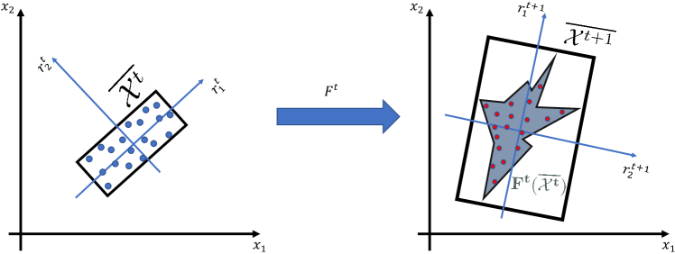
Figure 1: Using PCA to estimate the orientation of rectangles.

If we choose axis-aligned rectangles to over-approximate the reachable sets, then we can readily compute these sets recursively using the proposed BnB method in $\S$II. Suppose $\overline{\mathcal{X}}^{t}=[\ell^{t},u^{t}]$ has been computed. To compute $\overline{\mathcal{X}}^{t+1}=[\ell^{t+1},u^{t+1}]$, we must solve the optimization problems $\ell_{i}^{t+1}=\min_{x\in\overline{\mathcal{X}^{t}}}\{{e^{i}}^{\top}F^{t}(x)\},\quad u_{i}^{t+1}=-\min_{x\in\overline{\mathcal{X}^{t}}}\{-{e^{i}}^{\top}F^{t}(x)\},$ where $e^{i}$ is $i$-th standard basis vector. Axis-aligned rectangles, however, might be too conservative as they might not capture the shape of the true reachable sets accurately. To mitigate this conservatism, we propose to use rotated rectangles defined as $\overline{\mathcal{X}}^{t}=\{x\mid x=R^{t}y,\ y\in[\ell^{t},u^{t}]\}$ where $R^{t}$ is an orthonormal change-of-basis matrix from $x$ to $y$, and $\ell^{t},u^{t}$ are lower and upper bounds on $y$. This set representation can be incorporated into our BnB framework by simply branching in the $y$ space. Now it remains to determine $R^{t}$, $\ell^{t}$, and $u^{t}$.

Inspired by [39], we derive the rotation matrix $R^{t}$ at each time $t$ from sample trajectories. More precisely, suppose we have $p$ sample trajectories $\{x^{0,i},\cdots,x^{T,i}\}_{i=1}^{p}$. Then by applying PCA on the data points $\{x^{t,i}\}_{i=1}^{p}$, we obtain an orthonormal basis $R^{t}$ in which the sampled points are uncorrelated. Thus, we have $R^{t}=[r^{t,1},\cdots,r^{t,n_{x}}]$, where $r^{t,i}$ are the principal directions.

To determine $\ell^{t},u^{t}$, the following proposition shows that we can find these bounds recursively.

Proposition 1

For $i=1,2,\cdots,n_{x}$ define

$$\begin{split}\ell_{i}^{t+1}&=\min_{y\in[\ell^{t},u^{t}]}\{{r^{t+1,i}}^{\top}F^{t}(R^{t}y)\}\\ u_{i}^{t+1}&=-\min_{y\in[\ell^{t},u^{t}]}\{{-r^{t+1,i}}^{\top}F^{t}(R^{t}y)\}.\end{split}$$ (10)

Then, we have

$$F(\overline{\mathcal{X}}^{t})\subseteq\overline{\mathcal{X}}^{t+1}=\{x\mid x={R^{t+1}}y,\ y\in[\ell^{t+1},u^{t+1}]\}.$$

Proof:

Let $x\in F(\overline{\mathcal{X}}^{t})$. As $R^{t}$ is orthonormal, there exists a unique $y$ such that $x=R^{t+1}y$, so

$$y={R^{t+1}}^{\top}x=\begin{bmatrix}{r^{t+1,1}}^{\top}x,&\cdots,&{r^{t+1,n_{x}}}^{\top}x\end{bmatrix}^{\top}.$$

By definition in (10), we have

$$\ell^{t+1}_{i}=\min_{y\in[\ell^{t},u^{t}]}\{{r^{t+1,i}}^{\top}F^{t}(R^{t}y)\}\leq{r^{t+1,i}}^{\top}x=y_{i},$$

and

$$y_{i} \leq-\!\min_{y\in[\ell^{t},u^{t}]}\{{-r^{t+1,i}}^{\top}F^{t}(R^{t}y)\}\!=\!u_{i}^{t+1}.$$

∎

According to Proposition 1, to over-approximate the reachable set at time $t+1$ using rotated rectangles, we must solve the optimization problems in (10). We can solve these problems using the BnB framework of $\S$II provided that we can bound the Lipschitz constant of

$$J_{c}(y)=c^{\top}(A^{t}R^{t}y+B^{t}f(R^{t}y)).$$ (11)

We propose an extension of LipSDP that computes guaranteed bounds on the Lipschitz constant of $J_{c}$. To state the result, we define

$$\begin{split}A_{F}&=\begin{bmatrix}\mathrm{blkdiag}(W^{0}R^{t},\cdots,W^{L-1})&0_{N\times n_{L}}\end{bmatrix},\\ B_{F}&=\begin{bmatrix}0_{N\times n_{0}}&I_{N}\end{bmatrix},\\ C_{F}&=\begin{bmatrix}c^{\top}A^{t}R^{t}&0_{1\times(N-n_{L})}&c^{\top}B^{t}W^{L}\end{bmatrix},\\ D_{F}&=\begin{bmatrix}I_{n_{0}}&0_{n_{0}\times N}\end{bmatrix},\end{split}$$ (12)

where $N=\sum_{i=1}^{L}n_{i}$ denotes the number of neurons.

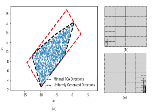
Figure 2: (a) Polyhedral approximation of the reachable set for the robotic arm example. (b-c) Input space partitions made by the branch sub-routine on two directions ($c=[-0.994,-0.104]^{\top}$ and $c=[0.994,0.104]^{\top}$) for the robotic arm task.

Theorem 1

Consider an $L$-layer fully connected neural network described by (7). Suppose the activation functions are slope-restricted in the sector $[\alpha,\beta]$. Define $A_{F},B_{F},C_{F},D_{F}$ as in (12). Define the matrix

$$\begin{bmatrix}A_{F}\\ B_{F}\end{bmatrix}^{\top}\!\begin{bmatrix}-2\alpha\beta T&(\alpha\!+\!\beta)T\\ (\alpha\!+\!\beta)T&-2T\end{bmatrix}\begin{bmatrix}A_{F}\\ B_{F}\end{bmatrix}\!+\!C_{F}^{\top}C_{F}\!-\!\rho D_{F}^{\top}D_{F},$$ (13)

where $\rho>0$ and $T$ is a diagonal positive semidefinite matrix of size $n\times n$. If (13) is negative semidefinite for some $(\rho,T)$, then $\sqrt{\rho}$ is a Lipschitz constant of $J_{c}(y)=c^{\top}(A^{t}R^{t}y+B^{t}f(R^{t}y))$ in $\ell_{2}$ norm.

Proof:

Starting from the compositional representation of the neural network in (7), we can write $J_{c}$ as

$$\xi^{0} =y,\quad\xi^{1}=\phi(W^{0}R^{t}\xi^{0}),$$

$$\xi^{k+1} =\phi(W^{k}\xi^{k}),\quad k=1,\cdots,L-1,$$

$$J_{c}(y) =c^{\top}A^{t}R^{t}\xi^{0}+c^{\top}B^{t}W^{L}\xi^{L}.$$

Following [34], we can compactly write these equations as

$$B_{F}\xi=\phi(A_{F}\xi),\quad J_{c}(y)=C_{F}\xi,$$ (14)

where $\xi=[{\xi^{0}}^{\top}\cdots{\xi^{L}}^{\top}]^{\top}$. Define the matrices

$$M^{1} =\begin{bmatrix}A_{F}\\ B_{F}\end{bmatrix}^{\top}\begin{bmatrix}-2\alpha\beta T&(\alpha\!+\!\beta)T\\ (\alpha\!+\!\beta)T&-2T\end{bmatrix}\begin{bmatrix}A_{F}\\ B_{F}\end{bmatrix},$$

$$M^{2} =C_{F}^{\top}C_{F}\!-\!\rho D_{F}^{\top}D_{F}.$$

Suppose $\overline{y}$ and $\overline{\xi}$ satisfy (14). Left and right multiply $M^{1}$ by $(\xi-\overline{\xi})^{\top}$ and $(\xi-\overline{\xi})$, respectively to obtain

Algorithm 1 ReachLipBnB

Inputs: Set of initial states $\mathcal{X}^{0}$, Neural network $f$, System dynamics $A^{t},B^{t}$, Final horizon $h_{f}$, Number of trajectories $p$
Outputs: Reachable sets $\mathcal{Y}^{i}$ and corresponding rotation transformations $R^{i}$ for $i=1,\cdots,h_{f}$
Initialize: $\mathcal{Y}^{0}=\mathcal{X}^{0}$, $R^{0}=I_{n_{x}}$, Trajectories $\{x^{t,j}\}_{t=0}^{h_{f}},j=1,\cdots,p$.

1:for t $=0,1,\cdots,h_{f}-1$ do

2:     partitions $=\{\mathcal{Y}^{t}\}$

3:     directions = PCA($\{x^{t+1,j}\}_{j=1}^{p}$)

4:     $F^{t}(\cdot)=A^{t}R^{t}(\cdot)+B^{t}f(R^{t}(\cdot))$

5:     for $c$ in directions do

6:         $J=c^{\top}F^{t}$

7:         $L_{J}=\mathrm{LipSDP}(J)$

8:         $\mathrm{BUB}=\min_{j=1,\cdots,p}J(x^{t+1,j})$, $\mathrm{BLB}=-\infty$

9:         while $\mathrm{BUB}-\mathrm{BLB}>\varepsilon$ do

10:              Bound${}_{J,L_{J}}$(partitions)

11:              $\mathrm{BLB},\mathrm{BUB}\leftarrow$ (5)

12:              partitions = Prune(partitions, $\mathrm{BUB}$)

13:              partitions = Branch(partitions)               

14:     $\mathcal{Y}^{t+1}\leftarrow$ using (10)

15:     $R^{t+1}\leftarrow$ directions

$$(\xi-\overline{\xi})^{\top}M^{1}(\xi-\overline{\xi})=$$ (15)

$$\begin{bmatrix}A_{F}(\xi-\overline{\xi})\\ \phi(A_{F}\xi)-\phi(A_{F}\overline{\xi}))\end{bmatrix}^{\top}\begin{bmatrix}-2\alpha\beta T&(\alpha+\beta)T\\ (\alpha+\beta)T&-2T\end{bmatrix}\begin{bmatrix}\star\end{bmatrix}\geq 0$$

where the last inequality follows from the fact that $\phi$ is slope restricted [34]. Similarly, we can write

$$(\xi-\overline{\xi})^{\top}M^{2}(\xi-\overline{\xi})=(J(y)-J(\overline{y}))^{2}-\rho\|y-\overline{y}\|_{2}^{2},$$ (16)

By adding both sides of (15) and (16), we get

$$(\xi-\overline{\xi})^{\top}(M^{1}+M^{2})(\xi-\overline{\xi})\geq(J(y)-J(\overline{y}))^{2}\!-\!\rho\|y-\overline{y}\|_{2}^{2}$$

When the LMI in (13) is feasible, the left-hand side is non-positive, implying that the right-hand side is non-positive. Thus, $|J(y)-J(\overline{y})|\leq\sqrt{\rho}\|y-\overline{y}\|_{2}$. ∎

Remark 1

The trajectories used in the PCA can also provide us with a good initialization for $\mathrm{BUB}$ by choosing the maximum of the objective values evaluated at these points.

IV NUMERICAL RESULTS

In this section, we evaluate and compare our algorithm on three tasks with those of Reach-LP [33] and Reach-SDP [32]. The first problem is a 2-dimensional open-loop task and the rest are closed-loop reachability tasks. The experiments are conducted on an Intel Xeon W-2245 3.9 GHz processor with 64 GB of RAM. Throughout the experiments, we let $k_{b}$ be 512.

IV-A Robotic Arm

The first experiment is similar to the robotic arm test case from [19]. For this experiment, $10^{4}$ data points were generated and used to train a single-layer neural network with two inputs, two outputs, and 50 hidden neurons. The network takes $\theta^{1}$ and $\theta^{2}$ as input and maps it to all the possible points in $x-y$ plane that the robot can reach. The input constraint is $\frac{\pi}{3}\leq\theta^{1},\theta^{2}\leq\frac{2\pi}{3}$.
Fig. 2 shows the results on this problem in two cases; (i) using PCA to generate the four directions and (ii) using 60 uniformly spaced vectors between $[0,2\pi]$. Fig. 2 also shows the resulting input space partitioning for two directions.

	ReachLP	ReachSDP	ReachLipBnB
$\varepsilon$	-	-	0.1	0.01	0.001
Time[s]	0.89	2.01	0.989 $\pm$ 0.058	1.204 $\pm$ 0.055	1.518 $\pm$ 0.066

Table I: Time comparison for different $\varepsilon$ for the double integrator experiment. The Reach-LP algorithm is run with GSG as the partitioner and CROWN as the propagator.

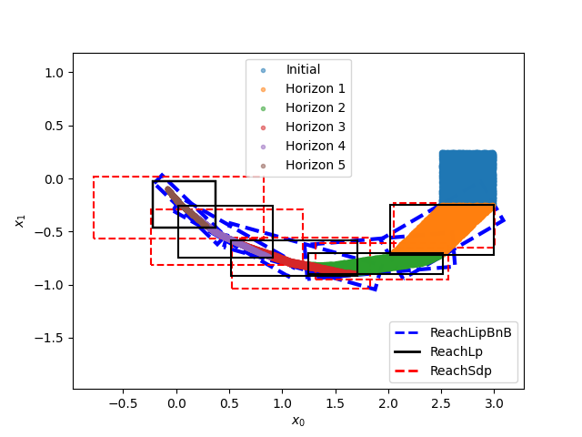
Figure 3: Double Integrator reachability analysis ($\varepsilon=0.01$).

IV-B Double Integrator

We consider the discrete-time double integrator system from [32], which can be written in the form of (8) with $A=\begin{bmatrix}1&1\\ 0&1\end{bmatrix}$, $B=\begin{bmatrix}0.5\\ 1\end{bmatrix}$. The control policy is a neural network that has been trained to approximate an MPC controller. We train a neural network that has an architecture of $2\times 10\times 5\times 1$ and run reachability analysis on this closed-loop system for five time steps and compare the results with [33, 32] in Fig. 3. The run time statistics of this experiment in Tables [I, II], are calculated over 100 runs of the algorithm reported as $\mu\pm\sigma$. Table I shows the results for different $\varepsilon$ tolerances.

IV-B1 Bound Refinement

We test the effect of bound refinement ($k_{v}=4$) on the performance of the algorithm. As reflected in Table II, bound refinement increases the run time of the algorithm but significantly reduces the number of total branches.

$\varepsilon$		0.1	0.01	0.001
OR	Run time[s]	0.989 $\pm$ 0.058	1.204 $\pm$ 0.055	1.518 $\pm$ 0.066
	Num total branches	1.1k	4.3k	8.8k
BR	Run time[s]	1.061 $\pm$ 0.056	1.574 $\pm$ 0.069	2.384 $\pm$ 0.068
	Num total branches	0.5k	2.3k	5.2k
LL	Run time[s]	0.949 $\pm$ 0.051	1.064 $\pm$ 0.055	1.226 $\pm$ 0.058
	Num total branches	0.2k	1.5k	2.9k

Table II: Time and memory comparison for different $\varepsilon$ for the double integrator between the original (OR), bound refinement (BR), and lower Lipschitz (LL). The total number of optimization problems solved is 20.

IV-B2 Low Lipchitz Network

To show the effect of the Lipschitz constant on our reachability task, we train a network with a lower Lipchitz constant using the method proposed in [40] and report the results in Table II. A lower Lipschitz constant would yield better lower bounds, hence allowing us to Prune more partitions, limiting the search space and reducing the overall run time.

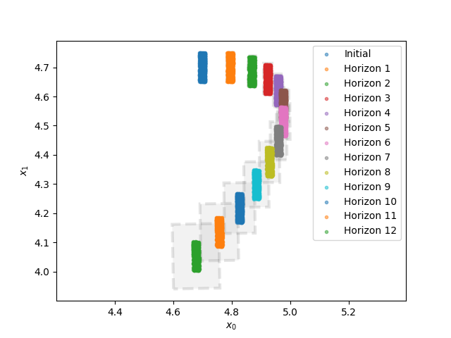
Figure 4: 6D Quadrotor reachability analysis. The grey area shows the over-approximations calculated by our method.

IV-C 6D Quadrotor

The 6D Quadrotor can be described using (9) with $A=I_{6\times 6}+\!\Delta t\times\begin{bmatrix}0_{3\times 3}&I_{3\times 3}\\ 0_{3\times 3}&0_{3\times 3}\end{bmatrix}$, $B=\!\Delta t\!\times\!\begin{bmatrix}&g&0&0\\ 0_{3\times 3}&0&-g&0\\ &0&0&1\end{bmatrix}^{\top}$, $u=\begin{bmatrix}\tan(\theta)\\ \tan(\phi)\\ \tau\end{bmatrix}$ and $c=\Delta t\times\begin{bmatrix}0_{5\times 1}\\ -g\end{bmatrix}$. Similar to the previous test case, an MPC controller is designed for the discretized closed-loop system (with $\Delta t=0.1$), and then a neural network is trained to approximate it. The neural network has an architecture of $6\times 32\times 32\times 3$. Fig. 4 shows the result of reachability analysis from an initial rectangle $[4.69,4.71]\times[4.65,4.75]\times[2.975,3.025]\times[0.9499,0.9501]\times[-0.0001,0.0001]\times[-0.0001,0.0001]$ for 12 time steps (equivalent to $1.2$s in the continuous time system).

V Conclusion

In this paper we proposed a branch-and-bound method for reachability analysis of neural networks, in which the bounding sub-routine is based on Lipschitz continuity arguments. The proposed algorithm is particularly efficient when the Lipschitz constant of the neural network is small. Several heuristics [40, 41] have been proposed to reduce the Lipschitz constant of neural networks during training. For future work, we will explore more effective heuristics to improve the overall performance of the algorithm.

References

- [1] Felix Berkenkamp, Matteo Turchetta, Angela Schoellig and Andreas Krause “Safe model-based reinforcement learning with stability guarantees” In Advances in neural information processing systems 30, 2017
- [2] Steven W Chen, Tianyu Wang, Nikolay Atanasov, Vijay Kumar and Manfred Morari “Large scale model predictive control with neural networks and primal active sets” In Automatica 135 Elsevier, 2022, pp. 109947
- [3] Steven Chen, Kelsey Saulnier, Nikolay Atanasov, Daniel D Lee, Vijay Kumar, George J Pappas and Manfred Morari “Approximating explicit model predictive control using constrained neural networks” In 2018 Annual American control conference (ACC), 2018, pp. 1520–1527 IEEE
- [4] Ahmed H Qureshi, Anthony Simeonov, Mayur J Bency and Michael C Yip “Motion planning networks” In 2019 International Conference on Robotics and Automation (ICRA), 2019, pp. 2118–2124 IEEE
- [5] Olalekan Ogunmolu, Xuejun Gu, Steve Jiang and Nicholas Gans “Nonlinear systems identification using deep dynamic neural networks” In arXiv preprint arXiv:1610.01439, 2016
- [6] Hongkai Dai, Benoit Landry, Lujie Yang, Marco Pavone and Russ Tedrake “Lyapunov-stable neural-network control” In arXiv preprint arXiv:2109.14152, 2021
- [7] Guy Katz, Clark Barrett, David L Dill, Kyle Julian and Mykel J Kochenderfer “Reluplex: An efficient SMT solver for verifying deep neural networks” In International conference on computer aided verification, 2017, pp. 97–117 Springer
- [8] Vincent Tjeng, Kai Xiao and Russ Tedrake “Evaluating robustness of neural networks with mixed integer programming” In arXiv preprint arXiv:1711.07356, 2017
- [9] Souradeep Dutta, Susmit Jha, Sriram Sankaranarayanan and Ashish Tiwari “Output range analysis for deep feedforward neural networks” In NASA Formal Methods Symposium, 2018, pp. 121–138 Springer
- [10] Brendon G Anderson, Ziye Ma, Jingqi Li and Somayeh Sojoudi “Tightened convex relaxations for neural network robustness certification” In 2020 59th IEEE Conference on Decision and Control (CDC), 2020, pp. 2190–2197 IEEE
- [11] Rudy Bunel, Alessandro De Palma, Alban Desmaison, Krishnamurthy Dvijotham, Pushmeet Kohli, Philip Torr and M Pawan Kumar “Lagrangian decomposition for neural network verification” In Conference on Uncertainty in Artificial Intelligence, 2020, pp. 370–379 PMLR
- [12] Alessandro De Palma, Rudy Bunel, Alban Desmaison, Krishnamurthy Dvijotham, Pushmeet Kohli, Philip HS Torr and M Pawan Kumar “Improved branch and bound for neural network verification via lagrangian decomposition” In arXiv preprint arXiv:2104.06718, 2021
- [13] Kaidi Xu, Huan Zhang, Shiqi Wang, Yihan Wang, Suman Jana, Xue Lin and Cho-Jui Hsieh “Fast and complete: Enabling complete neural network verification with rapid and massively parallel incomplete verifiers” In arXiv preprint arXiv:2011.13824, 2020
- [14] Panagiotis Kouvaros and Alessio Lomuscio “Towards Scalable Complete Verification of Relu Neural Networks via Dependency-based Branching.” In IJCAI, 2021, pp. 2643–2650
- [15] Shiqi Wang, Huan Zhang, Kaidi Xu, Xue Lin, Suman Jana, Cho-Jui Hsieh and J Zico Kolter “Beta-crown: Efficient bound propagation with per-neuron split constraints for neural network robustness verification” In Advances in Neural Information Processing Systems 34, 2021, pp. 29909–29921
- [16] Claudio Ferrari, Mark Niklas Mueller, Nikola Jovanović and Martin Vechev “Complete Verification via Multi-Neuron Relaxation Guided Branch-and-Bound” In International Conference on Learning Representations, 2021
- [17] Shiqi Wang, Kexin Pei, Justin Whitehouse, Junfeng Yang and Suman Jana “Formal security analysis of neural networks using symbolic intervals” In 27th USENIX Security Symposium (USENIX Security 18), 2018, pp. 1599–1614
- [18] Weiming Xiang, Hoang-Dung Tran, Xiaodong Yang and Taylor T Johnson “Reachable set estimation for neural network control systems: A simulation-guided approach” In IEEE Transactions on Neural Networks and Learning Systems 32.5 IEEE, 2020, pp. 1821–1830
- [19] Michael Everett, Golnaz Habibi and Jonathan P How “Robustness analysis of neural networks via efficient partitioning with applications in control systems” In IEEE Control Systems Letters 5.6 IEEE, 2020, pp. 2114–2119
- [20] Vicenc Rubies-Royo, Roberto Calandra, Dusan M Stipanovic and Claire Tomlin “Fast neural network verification via shadow prices” In arXiv preprint arXiv:1902.07247, 2019
- [21] Joseph A Vincent and Mac Schwager “Reachable polyhedral marching (rpm): A safety verification algorithm for robotic systems with deep neural network components” In 2021 IEEE International Conference on Robotics and Automation (ICRA), 2021, pp. 9029–9035 IEEE
- [22] Arnold Neumaier “The wrapping effect, ellipsoid arithmetic, stability and confidence regions” In Validation numerics Springer, 1993, pp. 175–190
- [23] Chao Huang, Jiameng Fan, Wenchao Li, Xin Chen and Qi Zhu “ReachNN: Reachability analysis of neural-network controlled systems” In ACM Transactions on Embedded Computing Systems (TECS) 18.5s ACM New York, NY, USA, 2019, pp. 1–22
- [24] Radoslav Ivanov, James Weimer, Rajeev Alur, George J Pappas and Insup Lee “Verisig: verifying safety properties of hybrid systems with neural network controllers” In Proceedings of the 22nd ACM International Conference on Hybrid Systems: Computation and Control, 2019, pp. 169–178
- [25] Souradeep Dutta, Xin Chen and Sriram Sankaranarayanan “Reachability analysis for neural feedback systems using regressive polynomial rule inference” In Proceedings of the 22nd ACM International Conference on Hybrid Systems: Computation and Control, 2019, pp. 157–168
- [26] Michael Everett, Bjorn Lutjens and Jonathan P How “Certified Adversarial Robustness for Deep Reinforcement Learning” In arXiv preprint arXiv:2004.06496, 2020
- [27] Nicholas Rober, Michael Everett and Jonathan P How “Backward Reachability Analysis for Neural Feedback Loops” In arXiv preprint arXiv:2204.08319, 2022
- [28] Hoang-Dung Tran, Patrick Musau, Diego Manzanas Lopez, Xiaodong Yang, Luan Viet Nguyen, Weiming Xiang and Taylor Johnson “NNV: A tool for verification of deep neural networks and learning-enabled autonomous cyber-physical systems” In International Conference on Computer-Aided Verification, 2020
- [29] Kyle D Julian and Mykel J Kochenderfer “Reachability analysis for neural network aircraft collision avoidance systems” In Journal of Guidance, Control, and Dynamics 44.6 American Institute of AeronauticsAstronautics, 2021, pp. 1132–1142
- [30] Chelsea Sidrane, Amir Maleki, Ahmed Irfan and Mykel J Kochenderfer “Overt: An algorithm for safety verification of neural network control policies for nonlinear systems” In Journal of Machine Learning Research 23.117, 2022, pp. 1–45
- [31] Xiaowu Sun, Haitham Khedr and Yasser Shoukry “Formal verification of neural network controlled autonomous systems” In Proceedings of the 22nd ACM International Conference on Hybrid Systems: Computation and Control, 2019, pp. 147–156
- [32] Haimin Hu, Mahyar Fazlyab, Manfred Morari and George J Pappas “Reach-SDP: Reachability Analysis of Closed-Loop Systems with Neural Network Controllers via Semidefinite Programming” In arXiv preprint arXiv:2004.07876, 2020
- [33] Michael Everett, Golnaz Habibi and Jonathan P How “Efficient reachability analysis of closed-loop systems with neural network controllers” In 2021 IEEE International Conference on Robotics and Automation (ICRA), 2021, pp. 4384–4390 IEEE
- [34] Mahyar Fazlyab, Alexander Robey, Hamed Hassani, Manfred Morari and George Pappas “Efficient and accurate estimation of lipschitz constants for deep neural networks” In Advances in Neural Information Processing Systems, 2019, pp. 11427–11438
- [35] Navid Hashemi, Justin Ruths and Mahyar Fazlyab “Certifying Incremental Quadratic Constraints for Neural Networks” In arXiv preprint arXiv:2012.05981, 2020
- [36] Rudy R Bunel, Ilker Turkaslan, Philip Torr, Pushmeet Kohli and Pawan K Mudigonda “A unified view of piecewise linear neural network verification” In Advances in Neural Information Processing Systems 31, 2018
- [37] Stephen Boyd and Jacob Mattingley “Branch and bound methods” In Notes for EE364b, Stanford University Citeseer, 2007, pp. 2006–07
- [38] Nathanaël Fijalkow, Joël Ouaknine, Amaury Pouly, João Sousa-Pinto and James Worrell “On the decidability of reachability in linear time-invariant systems” In Proceedings of the 22nd ACM International Conference on Hybrid Systems: Computation and Control, 2019, pp. 77–86
- [39] Olaf Stursberg and Bruce H Krogh “Efficient representation and computation of reachable sets for hybrid systems” In International Workshop on Hybrid Systems: Computation and Control, 2003, pp. 482–497 Springer
- [40] Henry Gouk, Eibe Frank, Bernhard Pfahringer and Michael J Cree “Regularisation of neural networks by enforcing lipschitz continuity” In Machine Learning 110.2 Springer, 2021, pp. 393–416
- [41] Nitish Srivastava, Geoffrey Hinton, Alex Krizhevsky, Ilya Sutskever and Ruslan Salakhutdinov “Dropout: a simple way to prevent neural networks from overfitting” In The journal of machine learning research 15.1 JMLR. org, 2014, pp. 1929–1958