Verifying a stochastic model for the spread of a SARS-CoV-2-like infection: opportunities and limitations

Abstract

There is a growing interest in modeling and analyzing the spread of diseases like the SARS-CoV-2 infection using stochastic models. These models are typically analyzed quantitatively and are not often subject to validation using formal verification approaches, nor leverage policy syntheses and analysis techniques developed in formal verification.

In this paper, we take a Markovian stochastic model for the spread of a SARS-CoV-2-like infection. A state of this model represents the number of subjects in different health conditions. The considered model considers the different parameters that may have an impact on the spread of the disease and exposes the various decision variables that can be used to control it. We show that the modeling of the problem within state-of-the-art model checkers is feasible and it opens several opportunities. However, there are severe limitations due to i) the espressivity of the existing stochastic model checkers on one side, and ii) the size of the resulting Markovian model even for small population sizes.

1 Introduction

The recent COVID-19 pandemic highlighted the importance to develop reliable models to study, predict and control the evolution and spread of diseases. Several analytical models have been proposed in the literature [3, 15, 1, 5, 11, 10, 4, 16, 24]. All these models are deterministic and aims at capturing the disease dynamics. These studies have been complemented with studies proposing stochastic models, that differently from deterministic ones, allows to derive richer set of informations like e.g. show converge to a disease-free state even if the corresponding deterministic models converge to an endemic equilibrium [2]; computing the probability of an outbreak, the distribution of the final size of a population or the expected duration of an epidemic [5, 22]; computing the probability of transition between different state of COVID-19-affected patients based on the age class [25]; or evaluating the effects of lock-down policies [21]. Recently, the evolution of diseases has also been modeled with stochastic models in form of Markov Processes [6, 1, 19]. The use of stochastic models opens for the possibility to use Stochastic Model Checking techniques to i) validate the model using probabilistic temporal properties of the model as well as compute quantitative measures of the degree of satisfaction of a given temporal property [20]; ii) evaluate the effects of a strategy on a population during the evolution of a disease [8, 7]. The work in [19] describes a stochastic compartmental model (the population has been broken down into several compartments) for the spread of COVID-19like diseases, with some preliminary results on the use of stochastic model checking techniques to analyze a simplified version of the epidemic model.

In this paper we make the following contributions. First, we consider the epidemic model presented in [19] and we show how to encode it into languages suitable for being analyzed with state-of-the-art stochastic model checkers. To this extent, we developed a C++ open source tool that given the parameters of the epidemic model is able to generate models in the PRISM formalism [17] to be then analyzed by tools supporting that formalism (e.g. the PRISM [17] and the STORM [14] model checkers). Second, we show that the encoding of the considered model in the language accepted by model checkers is out of the espressivity capabilities of the input languages, and even for small population sizes it results in very large files that easily reach unacceptable timings for the storage and parsing of such models, thus preventing any further analysis. To this extent, we modified the developed tool to link with the STORM model checker to pass the model directly in memory without the use of intermediate files. Third, we used the developed tool to study the model with increasing population sizes, analyzing the models against given temporal properties, and evaluating the effects of different control policies. These results show that the approach is feasible, but they confirm the scalability issues first noticed in [18, 12], and pose challenges to the community to address large population sizes on one hand, and espressivity requirements on the input languages, on the other hand, to facilitate the specification of such complex mathematical models.

This paper is organized as follows. In Section 2 we briefly summarize the basic concepts. In Section 3 we discuss the model presented in [19] and we show how to compute the probabilistic transition function. In Section 4 we describe the tools and the experiments carried out. In Section 5 we discuss the related works, an finally in Section 6 we draw conclusions and discuss possible future works.

2 Background

An Markov Decision Process (MDP) is a tuple $\langle S,S_{I},A,T,R\rangle$ where $S$ is a finite set of states, $S_{I}\subseteq S$ is the set of initial states, $A$ is a finite set of actions (i.e. control variables), $T:S\rightarrow 2^{A\times S\times\mathbb{R}}$ is the transition probability function that associates to a state $s\in S$, an action $a\in A$ the probability $p$ to end up in state $s^{\prime}$, $R:S\times A\rightarrow\mathbb{R}$ is the reward function, giving the expected immediate reward $r$ gained by for taking action $a\in A$ in state $s\in S$ (we remark that, in many cases there is no reward function). A Discrete Time Markov Chain (DTMC) is an MDP such that in each state $s\in S$ there is only one action to be considered with an associated probability to end-up in a state $s^{\prime}\in S$ (i.e. there is a single probability distribution over successor states). Partially Observable MDPs, extend MDPs by a set of observations and label every state with one of these observations. Thus, the states labeled by the same observation must be considered undistinguishable.

Several formalism have been proposed to specify (PO)MDPs and DTMCs. We refer to [14] for a thorough overview. In the following we briefly describe the PRISM language [17] supported by the PRISM and STORM stochastic model checkers. The PRISM language is a simple state-based language such that i) the user specifies variables with a finite domain (a complete assignment of a value to these variables at any given time constitutes a possible state of the system); ii) the behavior is specified through commands of the form [action] guard -> prob_1 : update_1 + ... + prob_n : update_n where: guard is a predicate over all the variables in the model, each update_i describes a transition which the model can make if the guard is true (a transition specifies the new values of the variables, and is associated to the probability/rate prob_i to take that update), and to an optional annotation action (modeling a control variable). On a (PO)MDP/DTMC model one can check several kind of properties, like e.g., temporal logic formulas based on PCTL [13] (e.g., property $\operatorname{\mathbf{P}}_{<0.25}[\operatorname{\mathbf{F}}O_{k}=C]$ means the probability of reaching a state where the variable $O_{k}$ is equal to $C$ is less than 0.25), or compute the probability with which a system reaches a certain state (e.g., $\operatorname{\mathbf{P}}_{=?}[\operatorname{\mathbf{F}}O_{k}=C]$ to compute the probability to reach a state where $O_{k}$ is equal to $C$), or perform conditional probability and cost queries, or compute long-run average values (also known as steady-state or mean payoff values), or synthesize a policy to satisfy a certain PCTL property. We refer the reader to [13, 17, 14] for a thorough discussion of possible queries.

In the following, we denote with $n!=n\cdot(n-1)\cdot...\cdot 1$ the factorial (i.e. the permutations of $n$ elements), with $\binom{n}{k}=\frac{n!}{k!\cdot(n-k)!}$ the binomial coefficient, with $\mathbb{M}_{n,n_{1},n_{2},\dots,n_{k-1}}=\binom{n}{n_{1},n_{2},\dots,n_{k}}=\frac{n!}{\prod_{i=1}^{k}n_{i}!}$ the multinomial coefficient (i.e. the permutations with repetitions obtained computing all the permutations of $n$ elements taken from $k$ sets with $n_{1},n_{2},\dots,n_{k}$ elements such that $n_{k}=n-\sum_{i=1}^{k-1}n_{i}$), and with $\mathcal{B}(N,p)_{X}=\binom{N}{X}p^{X}(1-p)^{N-X}$ the binomial probability distribution function where $X$ is the total number of successes, $p$ is the probability of success on an individual trial, and $N$ is the number of trials.

3 A stochastic model for SARS-CoV-2-like infection’s spread

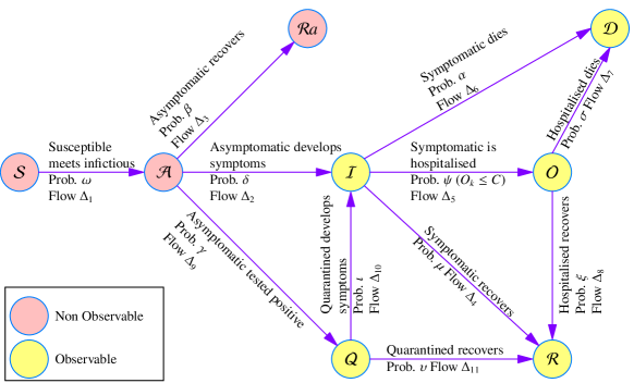
Figure 1: Transitions between the different states of a single subject of the entire population.

We model a subject of the population as a stochastic discrete–time system with 8 states, as illustrated in Figure 1, each representing a possible state of the subject: the susceptible $S$, infected $I$, recovered $R$, asymptomatic $A$ (i.e., a group of infected people that do not exhibit symptoms but are infective), hospitalised $O$, dead $D$, recovered $Ra$ from an asymptomatic state, and the case of swab-tested people that are quarantined (denoted with $Q$) if they result positive. The evolution is observed at discrete time $k$ and each subject can belong to one of eight possible states. The subjects who are in a state at step $k$ will be denoted by a calligraphic letter (e.g., $\mathcal{S}_{k}$ is the set of susceptible subjects). Figure 2 reports the symbols used to denote the different sets, their cardinality (e.g., $S_{k}$ is the cardinality of $\mathcal{S}_{k}$) and the different probabilities governing the transition of a subject between the different sets. The states of the discrete–time Markov chain can be characterized by a vector $\vec{V}_{k}=\left[S_{k},A_{k},I_{k},R_{k},O_{k},D_{k},Q_{k},Ra_{k}\right]$ such that the values of all the different quantities are non-negative integers representing the cardinality of their respective sets.

Sets $S_{k}=\left|\mathcal{S}_{k}\right|$ $\text{N. of susceptible sub. $\mathcal{S}_{k}$ at step }k,$ $A_{k}=\left|\mathcal{A}_{k}\right|$ $\text{N. of asymptomatic sub. $\mathcal{A}_{k}$ at step }k,$ $I_{k}=\left|\mathcal{I}_{k}\right|$ $\text{N. of symptomatic sub. $\mathcal{I}_{k}$ at step }k,$ $R_{k}=\left|\mathcal{R}_{k}\right|$ $\text{N. of recovered sub. $\mathcal{R}_{k}$ at step }k,$ $Ra_{k}=\left|\mathcal{R}a_{k}\right|$ $\text{N. of asympt. recovered sub. $\mathcal{R}a_{k}$ at step }k,$ $O_{k}=\left|\mathcal{O}_{k}\right|$ $\text{N. of hospitalised sub. $\mathcal{O}_{k}$ at step }k,$ $D_{k}=\left|\mathcal{D}_{k}\right|$ $\text{N. of deceased sub. $\mathcal{D}_{k}$ at step }k,$ $Q_{k}=\left|\mathcal{Q}_{k}\right|$ $\text{N. of quarantined sub. $\mathcal{Q}_{k}$ at step }k,$ $Q^{(R)}_{k}\!\!=\!\left|\mathcal{Q}^{(R)}_{k}\!\right|\!$ $\text{N. of quarantined sub. recovered $\mathcal{Q}^{(R)}_{k}$ at step }k.$ Deterministic Parameters $N$ $\text{Total number of subjects},$ $C$ $\text{Available beds in hospital facilities}.$ Probabilistic Parameters $\omega$ $\text{Prob. to contract the infection in one meeting},$ $\beta$ $\text{Prob. for an infectious asympt. sub. to recover},$ $\delta$ $\text{Prob. for an asympt. sub. to devel symptoms},$ $\mu$ $\text{Prob. for a symptomatic sub. to recover},$ $\alpha$ $\text{Prob. for a symptomatic sub. to die},$ $\sigma$ $\text{Prob. for an hospitalised sub. to die},$ $\xi$ $\text{Prob. for an hospitalised sub. to recover},$ $\gamma$ $\text{Prob. for a tested infectious sub. to be positive},$ $\psi$ $\text{Prob. for a symptomatic sub. to be hospitalised},$ $\iota$ $\text{Prob. that a quarantined sub. devel symptoms},$ $\upsilon$ $\text{Prob. that a quarantined sub. recovers}.$ Command Variables $M_{k}$ $\text{Num. of people met by any subject},$ $t_{k}$ $\text{Num. of people tested}.$

Figure 2: Summary of symbols.

This model is based on the following assumptions: i) the presence of a virus can be detected either if the subject starts to develop symptoms of the disease or when the subject is tested positive; ii) if a subject is tested positive (i.e. infectious) she/he becomes quarantiened until recovery; iii) a quarantined subject either recovers or develops the symptoms and becomes infectious; iv) a recovered subject cannot be re-infected; v) since it is not possible to distinguish a subject who is susceptible, asymptomatic or recovered without having developed symptoms, the states $\mathcal{S}$, $\mathcal{A}$, $\mathcal{R}a$ are not observable, while all the other states $\mathcal{Q}$, $\mathcal{I}$, $\mathcal{O}$, $\mathcal{D}$, $\mathcal{R}$ are observable; vi) the hospitals have a maximum capacity of $C\leq N$.

The elements of the vector $\vec{V}_{k}=\left[S_{k},A_{k},I_{k},R_{k},O_{k},D_{k},Q_{k},Ra_{k}\right]$ are subject to the following constraints: $S_{k}+A_{k}+I_{k}+R_{k}+Ra_{k}+Q_{k}+O_{k}+D_{k}=N,$ $O_{k}\leq C$. We denote with $\vec{\Delta v}=\vec{V_{k+1}}-\vec{V_{k}}\!=\![\Delta_{S},\Delta_{A},\Delta_{I},\Delta_{R},\Delta_{O},\Delta_{D},\Delta_{Q},\Delta_{Ra}]^{T}$ the change of the state vector from $\vec{V_{k}}$ to $\vec{V_{k+1}}$, such that the input/output flow from each state of Figure 1 is respected (i.e. $\Delta_{S}=-\Delta_{1}$, $\Delta_{A}=\Delta_{1}-\Delta_{2}-\Delta_{3}-\Delta_{9}$, $\Delta_{I}=\Delta_{10}+\Delta_{2}-\Delta_{4}-\Delta_{5}-\Delta_{6}$, $\Delta_{R}=\Delta_{4}+\Delta_{8}+\Delta_{11}$, $\Delta_{O}=\Delta_{5}-\Delta_{7}-\Delta_{8}$, $\Delta_{D}=\Delta_{6}+\Delta_{7}$, $\Delta_{Q}=\Delta_{9}-\Delta_{10}-\Delta_{11}$, $\Delta_{Ra}=\Delta_{3}$). Hereafter, we will refer to these equations with name balance equations. To ensure that different subjects in the different states of this model are non-negative we also enforce the following constraints: $\Delta_{1}\leq S_{k}$, $\Delta_{2}+\Delta_{3}+\Delta_{9}\leq A_{k}$, $\Delta_{10}+\Delta_{11}\leq Q_{k}$, $\Delta_{4}+\Delta_{5}+\Delta_{6}\leq I_{k}$, and $\Delta_{7}+\Delta_{8}\leq O_{k}$.

We denote by $l(\cdot)$ an assignment of variables: $\Delta_{i}=\delta_{i}$, for $i=1,\,\ldots,11$. For an assignment of variable $l(\cdot)$ we use $l(\cdot)\models\varphi$ to mean that the assignment $l(\cdot)$ satisfies formula $\varphi$. For instance, $l\left(\Delta_{4}=\delta_{4},\,\Delta_{8}=\delta_{8},\,\Delta_{11}=\delta_{11}\right)\models\Delta_{R}=\Delta_{4}+\Delta_{8}+\Delta_{11}$ means that the assignment $\delta_{4},\,\delta_{8},\,\delta_{22}$ to the variables $\Delta_{4}$, $\Delta_{8}$ and $\Delta_{11}$ satisfies balance equation $\Delta_{R}=\Delta_{4}+\Delta_{8}+\Delta_{11}$. We also introduce the following notations:

• $l_{1}$ is an assignment linking the variable $\Delta_{1}$ defined via $B_{1}$ as: $l_{1}$: $(\delta_{1}=-\Delta_{S})$;

• $l_{2}$ is a function linking the variables $\Delta_{2}$, $\Delta_{3}$ and $\Delta_{9}$ (with the variable $\Delta_{9}$ obtained via equation $B_{2}$, and the variable $\Delta_{3}$ obtained via equation $B_{8}$), defined as: $l_{2}$: $(\Delta_{2}=\delta_{2},\Delta_{3}=\Delta_{R_{a}},\,\,\Delta_{9}=\!-\!\Delta_{S}\!-\!\Delta_{A}\!-\!\Delta_{R_{a}}\!-\!\delta_{2})$;

• $l_{3}$ is a function linking $\Delta_{4},\Delta_{5},\Delta_{6}$ and given by: $l_{3}$: $(\Delta_{4}=\delta_{4},\Delta_{5}=\delta_{5},\Delta_{6}=\delta_{6})$;

• $l_{4}$ is an assignment linking the remaining variables defined as:
  $l_{4}$: $(\Delta_{7}=\Delta_{D}-\delta_{6},\,\,\Delta_{8}=\delta_{5}+\delta_{6}-\Delta_{D}-\Delta_{O},\,\,\Delta_{10}=\Delta_{I}-\delta_{2}+\delta_{4}+\delta_{5}+\delta_{6},\Delta_{11}=\Delta_{R}+\Delta_{D}+\Delta_{O}-\delta_{4}-\delta_{5}-\delta_{6})$;

• $l_{5}$, finally, assigns $(\Delta_{2}=\delta_{2},\Delta_{3}=\delta_{3},\Delta_{9}=\delta_{9})$.

Finally, we also consider the following terms: $C_{\beta,\delta}=(1-\beta-\delta)\geq 0$, $C_{\mu,\psi,\alpha}=(1-\mu-\psi-\alpha)\geq 0$, $C_{\sigma,\xi}=(1-\sigma-\xi)\geq 0$, $C_{\iota,\upsilon}=(1-\iota-\upsilon)\geq 0$.

The probability associated with a transition from state vector $\vec{V}_{k}$ to state vector $\vec{V}_{k+1}$, such that exactly $M_{k}$ encounters between susceptible subjects can happen and exactly $t_{k}$ tests are performed, denoted with $\mathrm{Pr}\{\vec{V}_{k+1}\!\left.\right\rvert\!\vec{V}_{k}\}$ can be computed as follows:

$$\mathrm{Pr}\{\vec{V}_{k+1}\!\left.\right\rvert\!\vec{V}_{k}\} =\mathrm{Pr}\{l_{1}\!\left.\right\rvert\!\vec{V}_{k}\}\cdot\displaystyle\sum_{\delta_{2}=0}^{-\Delta_{S}-\Delta_{A}-\Delta_{R_{a}}}\mathrm{Pr}\{l_{2}\!\left.\right\rvert\!\vec{V}_{k}\wedge l_{1}\}$$

$$\quad\quad\cdot\displaystyle\sum_{\delta_{4}=0}^{\delta_{2}-\Delta_{I}}\displaystyle\sum_{\delta_{5}=0}^{\delta_{2}-\Delta_{I}-\delta_{4}}\sum_{\delta_{6}=0}^{\delta_{2}-\Delta_{I}-\delta_{4}-\delta_{5}}\!\!\!\!\!\!\mathrm{Pr}\{l_{3}\!\left.\right\rvert\!\vec{V}_{k}\wedge l_{1}\wedge l_{2}\}$$ (1)

$$\quad\quad\quad\cdot\mathrm{Pr}\{l_{4}\!\left.\right\rvert\!\vec{V}_{k}\wedge l_{1}\wedge l_{2}\wedge l_{3}\}\!\!$$

where:

• $\mathrm{Pr}\{l_{1}\!\left.\right\rvert\!\vec{V}_{k}\}$ is the probability that exactly $\delta_{1}$ susceptible become asymptomatic, and is computed as $\mathrm{Pr}\{l_{1}\!\left.\right\rvert\!\vec{V}_{k}\}=\mathcal{B}(S_{k},\mathrm{Pr}\{g_{k}\!\left.\right\rvert\!\vec{V}_{k}\}_{M_{k}})_{-\Delta_{S}}$ where, and $\mathrm{Pr}\{g_{k}\!\left.\right\rvert\!\vec{V}_{k}\}_{M_{k}}=1-\left(\!1\!-\!\frac{\omega A_{k}}{N\!-\!D_{k}\!-\!I_{k}\!-\!O_{k}\!-\!Q_{k}}\right)^{M_{k}}$.

• $\mathrm{Pr}\{l_{2}\!\left.\right\rvert\!\vec{V}_{k}\wedge l_{1}\}$ is defined as $\displaystyle\sum_{H=\delta_{9}}^{t_{k}}\mathrm{Pr}\{s_{H}\}\sum_{F=0}^{\delta_{9}}\rho(\delta_{2},\delta_{3}\!+\!F,\vec{V}_{k})\binom{A_{k}}{H}^{-1}K$ where $t_{k}$ are the tests performed in the transition from $\vec{V}_{k}$ to $\vec{V}_{k+1}$, $K=\binom{\delta_{3}+F}{F}\binom{A_{k}-(\delta_{2}+\delta_{3}+F)}{\delta_{9}-F}\binom{\delta_{2}}{H-\delta_{9}}$, $\rho(\delta_{2},\delta_{3},\vec{V}_{k})=\frac{A_{k}!\,\beta^{\delta_{3}}\,\delta^{\delta_{2}}\,C_{\beta,\delta}^{A_{k}-\delta_{2}-\delta_{3}}}{\delta_{2}!\delta_{3}!(A_{k}-\delta_{2}-\delta_{3})!}$, and $\mathrm{Pr}\{s_{H}\}=\binom{N_{k}}{t_{k}}^{-1}\sum_{p=0}^{t_{k}}\binom{S_{k}+R_{a_{k}}}{t_{k}-p}\binom{A_{k}}{p}\mathcal{B}(p,\gamma)_{H}$.

• $\mathrm{Pr}\{l_{3}\!\left.\right\rvert\!\vec{V}_{k}\wedge l_{1}\wedge l_{2}\}$ is defined as

  $$\mathrm{Pr}\{l_{3}\!\left.\right\rvert\!\vec{V}_{k}\wedge l_{1}\wedge l_{2}\}= \begin{cases}0&\!\!\!\text{if }\delta_{4}+\delta_{5}+\delta_{6}>I_{k}\vee\delta_{5}>C-O_{k}\\ M(\delta_{4},\delta_{5},\delta_{6})&\!\!\!\text{if }\delta_{5}<C-O_{k}\wedge\delta_{4}+\delta_{5}+\delta_{6}\leq I_{k}\\ M^{\prime}(\delta_{4},\delta_{6})&\!\!\!\text{if }\delta_{5}=C-O_{k}\wedge\delta_{4}+\delta_{5}+\delta_{6}\leq I_{k}\end{cases}$$

  where $M(\delta_{4},\delta_{5},\delta_{6})=\mathbb{M}_{I_{k},\delta_{4},\delta_{5},\delta_{6}}\mu^{\delta_{4}}\,\psi^{\delta_{5}}\,\alpha^{\delta_{6}}\,C_{\mu,\psi,\alpha}^{I_{k}-\delta_{4}-\delta_{5}-\delta_{6}}$ and $M^{\prime}(\delta_{4},\delta_{6})=\sum_{h=0}^{I_{k}-\delta_{4}-\delta_{6}-(C-O_{k})}M(\delta_{4},(C-O_{k})+h,\delta_{6})$;

• $\mathrm{Pr}\{l_{4}\!\left.\right\rvert\!\vec{V}_{k}\wedge l_{1}\wedge l_{2}\wedge l_{3}\}$ is defined as $\zeta(\Delta_{D}\!-\!\delta_{6},\delta_{5}\!+\!\delta_{6}\!-\!\Delta_{D}\!-\!\Delta_{O},\vec{V}_{k})\cdot\chi(\Delta_{I}\!-\!\delta_{2}\!+\!\delta_{4}\!+\!\delta_{5}\!+\!\delta_{6},\Delta_{R}\!+\!\Delta_{D}\!+\!\Delta_{O}\!-\!\delta_{4}\!-\!\delta_{5}\!-\!\delta_{6},\vec{V}_{k})$ where $\zeta(\delta_{7},\delta_{8},\vec{V}_{k})=\mathbb{M}_{O_{k},\delta_{7},\delta_{8}}\sigma^{\delta_{7}}\,\xi^{\delta_{8}}\,C_{\sigma,\xi}$, and $\chi(\delta_{10},\delta_{11},\vec{V}_{k})=\mathbb{M}_{Q_{k},\delta_{10},\delta_{11}}\iota^{\delta_{10}}\,\upsilon^{\delta_{11}}\,C_{\iota,\,\upsilon}^{Q_{k}\!-\!\delta_{10}\!-\!\delta_{11}}$.

All the mathematical details and proofs to show the correctness of the above formulation for computing the probability of a transition from $\vec{V}_{k}$ to $\vec{V}_{k+1}$ subject to having exactly $M_{k}$ meetings and performing exactly $t_{k}$ tests for the model depicted in Figure 1 are out of the scope of this paper and can be found in [19].

Given the above definitions, we can compute the transitions and the associated probabilities from a state vector $\vec{V_{k}}$ given exactly $M_{k}$ encounters, and exactly $t_{k}$ tests by enumerating all possible configurations $\vec{V_{k+1}}$ that are compatible with the balance equations at page 2. Algorithm 1 in Appendix 0.A shows how to perform this enumeration.

The transitions from a state vector $\vec{V_{k}}$ subjected to encounters from a set of minimum encounters $M_{min}$ to a maximum of $M_{max}$ encounters, and tests from a minimum of $T_{min}$ to a maximum of $T_{max}$ can be computed by enumerating all possible $(m,t)$ such that $m\in[M_{min},M_{max}]$ and $t\in[T_{min},T_{max}]$ using previous algorithm (see Algorithm 2 in Appendix 0.A for details). These algorithms are the building blocks for computing the MDP for the full stochastic model for the spread of a SARS-CoV-2-like infection for a population of size $N$ such that each subject evolves as illustrated in Figure 1. The set of states of the MDP are all those vector states $\vec{V}_{k}=\left[S_{k},A_{k},I_{k},R_{k},O_{k},D_{k},Q_{k},Ra_{k}\right]$ such that they satisfy the constraint $S_{k}+A_{k}+I_{k}+R_{k}+O_{k}+D_{k}+Q_{k}+Ra_{k}=N$ for a population of $N$ subjects. The set of actions can be computed as $A=\{\langle M_{k},t_{k}\rangle\;|\;M_{k}\in[M_{min},M_{max}],t_{k}\in[t_{min},t_{max}]\}$, for the possibility to meet subjects from $M_{min}$ to $M_{max}$, and to perform tests from $t_{min}$ to $t_{max}$. The transition probability function $T=\{\langle\vec{V}_{k},\langle M_{k},t_{k}\rangle,\vec{V}_{k+1},\mathrm{Pr}\{\vec{V}_{k+1}\!\left.\right\rvert\!\vec{V}_{k}\}\rangle\;|\langle M_{k},t_{k}\rangle\in A,\vec{V}_{k}\in S,\langle\vec{V}_{k},\langle M_{k},t_{k}\rangle,\vec{V}_{k+1},\mathrm{Pr}\{\vec{V}_{k+1}\!\left.\right\rvert\!\vec{V}_{k}\}\rangle\in\textsc{Transitions}(\vec{V}_{k},M_{k},t_{k})\}$. Finally, $S_{I}\subseteq S$ is the set of initial states. In this model, we do not consider any reward function.

This framework allows for the application of several policies to control the (PO)MDP. To this extent, we see a policy as a function $\mathcal{P}(\vec{V}_{k})\rightarrow 2^{A}$ that associates with a state $\vec{V}_{k}$ a pair $\langle M_{k},t_{k}\rangle$ such that $M_{k}\in[M_{min},M_{max}]$ and $t_{k}\in[t_{min},t_{max}]$. This can be achieved by restricting the transition probability function to follow policy $\mathcal{P}$ as follows: $T=\{\langle\vec{V}_{k},\langle M_{k},t_{k}\rangle,\vec{V}_{k+1},\mathrm{Pr}\{\vec{V}_{k+1}\!\left.\right\rvert\!\vec{V}_{k}\}\rangle\;|\langle M_{k},t_{k}\rangle\in\mathcal{P}(\vec{V}_{k})\subseteq A,\vec{V}_{k}\in S,\langle\vec{V}_{k},\langle M_{k},t_{k}\rangle,\vec{V}_{k+1},\mathrm{Pr}\{\vec{V}_{k+1}\!\left.\right\rvert\!\vec{V}_{k}\}\rangle\in\textsc{Transitions}(\vec{V}_{k},M_{k},t_{k})\}$. Algorithms 1 and 2 can be easily adapted to restrict the actions to obey a given policy $\mathcal{P}(\vec{V}_{k})$. In particulara, it is sufficient in Algorithm 2 to replace the two nested for loops with a single loop over elements of a set of pairs $\langle m,t\rangle\in\mathcal{P}(\vec{V}_{k})$.

4 Experimenting with state-of-the-art stochastic model checkers

Once the (PO)MDP model has been built, one can convert it into the input format of a stochastic model checker like e.g. PRISM [17] or STORM [14], and use this model to verify PCTL [13] properties, for synthesizing policies satisfying a given PCTL property, to evaluate formally the effects of a policy, and to compute steady state probabilities.

To this extent, we have developed a C++ proof of concept open-source tool, name covid_tool. As an input, this tool receives (encoded in a json file) the population size $N$, all the probability parameters described in Figure 2, the $M_{min}$, $M_{max}$, $t_{min}$, $t_{max}$ and the hospital capacity $C$. The tool also accepts in input a set of possible initial states where for each initial state is fully specified by the respective $\vec{V}$. Moreover, to evaluate the possible effect of manually specified control policies, we integrated in the tools four policies $\mathcal{P}_{-1}$, $\mathcal{P}_{0}$, $\mathcal{P}_{1}$, and $\mathcal{P}_{2}$. $\mathcal{P}_{-1}$ corresponds to not applying any policy, and this results in generating all possible pairs in $A$ (see e.g., Algorithm 2). $\mathcal{P}_{0}$ is a constant policy that regardless of the state $\vec{V}_{k}$ returns a singleton element $\langle M,t\rangle$ (i.e., $\forall\vec{V}_{k}\in S.\mathcal{P}_{0}(\vec{V}_{k})=\{\langle M,t\rangle\}$). Policies $\mathcal{P}_{1}$ and $\mathcal{P}_{2}$ have the following form $\mathcal{P}(\vec{V}_{k})=\{\langle M_{k},t\rangle|M_{k}=\mathcal{F}(\vec{V}_{k}),t\in[t_{min},t_{max}]\}$ where

$$\mathcal{F}(\vec{V}_{k})\!=\!\begin{cases}M_{max}&\text{if }f(\vec{V}_{k})\leq T_{\downarrow}\\ M_{min}&\text{if }f(\vec{V}_{k})\geq T_{\uparrow}\\ M_{max}\!+\!\left(M_{min}\!-\!M_{max}\right)\frac{f(\vec{V}_{k})-T_{\downarrow}}{T_{\uparrow}-T_{\downarrow}}&\text{otherwise}.\end{cases}\!\!$$ (2)

$\mathcal{P}_{1}$ uses $f(\vec{V}_{k})=I_{k}+O_{k}/(N-D_{k})$ while $\mathcal{P}_{2}$ uses $f(\vec{V}_{k})=A_{k}/(N-D_{k})$. In $\mathcal{P}_{1}$ when the percentage of the number of symptomatic and hospitalized patients over the living population is below the threshold $T_{\downarrow}$, we impose no restrictions for social life. If this number is above a threshold $T_{\uparrow}$, we adopt the maximum restriction (the minimum value $M_{min}$ for $M$). Otherwise we adopt a linear interpolation between the minimum and the maximum values of $M$. $\mathcal{P}_{2}$ is similar to $\mathcal{P}_{1}$, but here we consider the ratio between asymptomatic infected subjects and the living population. The tool and all the material to reproduce the experiments reported hereafter are available at https://bitbucket.org/luigipalopoli/covd˙tool.

This tool uses Algorithms 1 and 2 to build the MDP for the model of Figure 1, and the respective adaptation of such algorithms to generate the DTMCs resulting from the application of a given pre-defined policy $\mathcal{P}$. Among the different possibilities this tool provides, we highlight here the ability to generate a (PO)MDP symbolic model as accepted by PRISM and STORM. The symbolic model encodes the state vector $\vec{V}$ with 8 integer variables (S, A, I, R, O, D, Q, Ra) with values ranging from 0 to $N$. We encode actions with a label action_m_t for meeting exactly $m$ subjects and performing exactly $t$ tests. Then using Algorithm 1 to compute the possible next states and respective probabilities. The tool is also able to generate a symbolic Partially Observable Markov Decision Problems in PRISM format by specifying that the S, A, Ra are not observable. Moreover, the tool can handle two cases, the full model with all the eight states as per Figure 1, and a simplified model that does not considers quarantined and the possibility to recover from asymptomatic state (that corresponds to a SAIROD model). We introduced this possibility for two main reasons. First, the SAIROD model has been already studied, and it is easier to retrieve the parameters governing the behavior [11]. Second, as we will see later on, the full model is subject to scalability issues much quickly than the simple SAIROD one. Listing 1 is an excerpt of a simple PRISM model corresponding to a population composed of 10 subjects.

⬇

mdp // The kind of model

module covid_mdp // The main module

// The variables

nS : [0..10]; nA : [0..10]; nI : [0..10]; nR : [0..10]; nO : [0..10]; nD : [0..10];

… // omitted for lack of space

[act_M_is_5] ((nS = 0) & (nA = 0) & (nI = 0) & (nR = 0) & (nO = 1) & (nD = 9)) ->

0.5 : (nS’ = 0) & (nA’ = 0) & (nI’ = 0) & (nR’ = 1) & (nO’ = 0) & (nD’ = 9)

+ 0.2 : (nS’ = 0) & (nA’ = 0) & (nI’ = 0) & (nR’ = 0) & (nO’ = 1) & (nD’ = 9)

+ 0.3 : (nS’ = 0) & (nA’ = 0) & (nI’ = 0) & (nR’ = 0) & (nO’ = 0) & (nD’ = 10);

… // omitted for lack of space

endmodule

init // The set of initial states

( (nS = 7) & (nA = 3) & (nI = 0) & (nR = 0) & (nO = 0) & (nD = 0)

| (nS = 9) & (nA = 1) & (nI = 0) & (nR = 0) & (nO = 0) & (nD = 0) )

endinit

Listing 1: Excerpt of a PRISM file generated for a SAIROD model with a population of 10 individuals. The entire file is about 103Mb on disk.

$N$	$C$	$P_{\textit{min}}$	$P_{\textit{max}}$	Creation of $T$ (s)	STORM model creation (s)	STORM model checking (s)
5	1	0.250	0.312	0.088	0.297	0.005
10	1	0.260	0.346	25.161	58.705	56.955
15	1	0.264	0.382	1118.465	3205.290	33.257
20	1		memout
10	2	0.005	0.019	36.080	103.292	2.191
15	3			memout

Table 1: Experiments using the extended model, no policy ($\mathcal{P}_{-1}$).

The generation of models in PRISM language is subject to severe efficiency and espressivity problems. First, the PRISM language can represent symbolically the transitions once the $\mathrm{Pr}\{\vec{V}_{k+1}\!\left.\right\rvert\!\vec{V}_{k}\}$ are pre-computed for each transition, but there is no efficient way to encode $\mathrm{Pr}\{\vec{V}_{k+1}\!\left.\right\rvert\!\vec{V}_{k}\}$ in the language due to the limited espressivity of the PRISM language (the involved math is not supported by the language). A possibility that we considered was to build a defined symbols to represent the $\mathrm{Pr}\{\vec{V}_{k+1}\!\left.\right\rvert\!\vec{V}_{k}\}$ for all possible values of the $\vec{V}_{k}$, $M_{k}$, and $t_{k}$, however the resulting file will be huge (larger than a gigabyte) even for a very small population ( $<10$ subjects). Thus, we ended up pre-computing such probabilities, and associating the resulting value with each transition. The size of the file is problematic for two reasons: first problem is a storage problem. Second problem, assuming the huge file has been generated successfully, the PRISM and STORM model checkers require a large amount of memory and huge timing (days) to parse the file before even starting verification on modern high-performance computers equipped with large memory (Terabytes). Here we remark that STORM is slightly more efficient than PRISM in handling large input files. This might be due to a number of reasons, notably the fact that STORM uses an efficient C++ parser, while PRISM uses Java. To overcome these limitations, we considered two directions. First, we considered the possibility to generate the explicit transition matrix files in the different formats accepted by the STORM and PRISM model checkers (the generated files with this flow are smaller than the symbolic approach, but still large and requiring large computation and memory to handle them). Second, we followed the direction to have a more strict integration with the model checker by linking the model checker in memory (thus avoiding intermediate file generation). In particular, we did a tight integration with the STORM model checker by directly building in memory the data structures to enable model checking. We have chosen STORM for two main reasons. Fist, it is written in C++ while PRISM is written in Java. Second, STORM provides a clear API to facilitate the integration in other tools. Currently, we are only building the sparse matrix representation [14], and thus we are limited to the verification capabilities by STORM with this model representation. (See https://www.stormchecker.org/ for further details.)

All the experiments have been executed on a cluster equipped with 112 Intel(R) Xeon(R) CPU cores 2.20GHz and 256Gb of RAM. We considered a memory limit of 256GB and a CPU time limit of 5400 seconds.

	Policy	$N$	$C$	$P$	Creation of $T$ (s)	STORM model creation (s)	STORM model checking (s)
ConstLow	$\mathcal{P}_{0}$	5	1	0.280	0.088	0.178	0.001
	$\mathcal{P}_{0}$	10	1	0.300	25.111	33.044	0.170
	$\mathcal{P}_{0}$	15	1	0.308	1131.249	988.710	5.031
	$\mathcal{P}_{0}$	10	2	0.011	36.010	49.453	0.301
	$\mathcal{P}_{0}$	15	3	0.0006	2371.702	2179.716	16.505
	$\mathcal{P}_{0}$	20	4		memout
ConstHigh	$\mathcal{P}_{0}$	5	1	0.280	0.088	0.175	0.001
	$\mathcal{P}_{0}$	10	1	0.300	25.032	33.642	0.182
	$\mathcal{P}_{0}$	15	1	0.308	1130.826	956.313	5.050
	$\mathcal{P}_{0}$	20	1		timeout
	$\mathcal{P}_{0}$	10	2	0.011	35.977	48.314	0.304
	$\mathcal{P}_{0}$	15	3	0.308	1130.826	956.313	5.051
	$\mathcal{P}_{0}$	20	4		timeout
Adapt1	$\mathcal{P}_{1}$	5	1	0.280	0.088	0.179	0.001
	$\mathcal{P}_{1}$	10	1	0.300	25.279	34.985	0.181
	$\mathcal{P}_{1}$	15	1	0.308	1132.725	957.143	5.005
	$\mathcal{P}_{1}$	20	1		memout
	$\mathcal{P}_{1}$	10	2	0.011	35.885	49.046	0.301
	$\mathcal{P}_{1}$	15	3			timeout
Adapt1	$\mathcal{P}_{2}$	5	1	0.280	0.088	0.187	0.001
	$\mathcal{P}_{2}$	10	1	0.300	25.062	32.684	0.184
	$\mathcal{P}_{2}$	15	1	0.308	1124.658	968.644	5.735
	$\mathcal{P}_{2}$	20	1		memout
	$\mathcal{P}_{2}$	10	2	0.011	35.931	48.781	0.306
	$\mathcal{P}_{2}$	15	3	0.0006	2528.367	2473.946	15.958
	$\mathcal{P}_{2}$	20	4		timeout
Adapt2	$\mathcal{P}_{1}$	5	1	0.280	0.087	0.179	0.001
	$\mathcal{P}_{1}$	10	1	0.300	25.048	32.583	0.169
	$\mathcal{P}_{1}$	15	1	0.308	1134.407	974.875	5.013
	$\mathcal{P}_{1}$	20	1		memout
	$\mathcal{P}_{1}$	10	2	0.011	35.885	48.797	0.316
	$\mathcal{P}_{1}$	15	3			timeout
Adapt2	$\mathcal{P}_{2}$	5	1	0.280	0.088	0.183	0.001
	$\mathcal{P}_{2}$	10	1	0.300	25.080	32.528	0.181
	$\mathcal{P}_{2}$	15	1	0.308	1124.280	949.528	5.051
	$\mathcal{P}_{2}$	20	1		memout
	$\mathcal{P}_{2}$	10	2	0.280	0.088	0.347	0.001
	$\mathcal{P}_{2}$	15	3			timeout

Table 2: Experiments using the extended model, policies $\mathcal{P}_{0}$, $\mathcal{P}_{1}$ and $\mathcal{P}_{2}$.

We conducted experiments with varying population sizes $N$, hospital capacities $C$ and policies used. The values of $M_{\textit{min}}$ and $M_{\textit{max}}$ used were 1 and 5, respectively. The values of $t_{\textit{min}}$ and $t_{\textit{max}}$ used were 1 and 3, respectively. These values are reasonable for the population sizes we managed to consider (see the results later in this section). All the values of the parameters (e.g., transition probabilities) were based on discussions with experts. The precise values used in all these experiments can be found in the aforementioned bitbucket Git repository of the tool. We performed the experiments on two versions of the model: i) the “full” model described in previous section (the results are reported in Tables  1 and  2), and ii) the “reduced” model, which does not consider the possibility of entering in quarantine ($\mathcal{Q}$) and the possibility for an asymptomatic to recover ($\mathcal{R}a$) (the results are reported in Tables  3 and  4 in the appendix). Moreover, we also considered the effects of the different considered policies. Tables  1 and  3 report the results for $\mathcal{P}_{-1}$, while Tables  2 and  4 show cases for policies $\mathcal{P}_{0}$, $\mathcal{P}_{1}$ and $\mathcal{P}_{2}$. In the experiments with policies $\mathcal{P}_{0}$, $\mathcal{P}_{1}$, $\mathcal{P}_{2}$ we considered the verification of the PCTL formula $\operatorname{\mathbf{P}}_{=?}[\operatorname{\mathbf{F}}O=C]$ (i.e. the probability of eventually reaching a state in which the hospital is saturated), while in the experiments with $\mathcal{P}_{0}$, we find minimum and maximum probabilities ($\operatorname{\mathbf{P}}_{min=?}[\operatorname{\mathbf{F}}O=C]$ and $\operatorname{\mathbf{P}}_{max=?}[\operatorname{\mathbf{F}}O=C]$, respectively). These properties were chosen given the interest of experts and decision makers of knowing the probabilities to saturate hospitals in different conditions. Constant policies ConstHigh and ConstLow use the $M$ values of 1 and 5, respectively. With Adapt1 we denote the adaptive policy with $T_{\downarrow}=0.1$ and $T_{\uparrow}=0.5$. Adapt2 denotes the adaptive policy with $T_{\downarrow}=0.05$ and $T_{\uparrow}=0.15$.

For each experiment we report: i) the time in seconds required to build the complete transition matrix with the approach described in the previous section; ii) the time in seconds to fill and build the model in memory within the STORM model checker; iii) the time in seconds required by STORM to model check the given property on the previously built model; iv) the computed probabilities for the considered properties.

The results in the tables clearly show that the time is mostly divided between computing the transition probability matrix and creating the STORM model (with checking the property taking relatively little time). This is due to the large number of states and transitions even for the small population sizes considered. With the hardware at our disposal, we mostly manage to deal with population sizes up to 25. All the experiments ran out of memory with larger values of $N$ while computing the transition probability matrix. We spent a significant engineering effort to limit this explosion trying to find efficient methods to represent states and transitions, as well as memorizing the result of the computation of the transition probabilities. However, despite this engineering effort, the large state space required reached easily the limits of the hardware at our disposal. We remark that, it is in principle possible to address scalability to large population size by considering a unit of population in the model as the representative of a (larger) number of people with a numerically quantifiable error (a similar approach has been discussed in [18], and is left as future work). The results also shows that, as expected, the probability of hospitals being saturated increases with increasing population sizes and decreases with greater hospital capacities.

We remark that, despite the limited scalability issues we encountered, this work constitute a basis to challenge stochastic model checkers along different directions (e.g., expressivity to allow for a concise representation of cases like this one, and efficiency to allow handle more realistic size scenarios). Moreover, it opens to the possibility to leverage the feature provided by stochastic model checkers to compute policies to achieve given properties of interest for a decision maker (although we have not yet experimented with this feature, and we will leave as future work).

5 Related works

There have been several works that addressed the problem of mathematically modeling the spread of diseases [3, 15, 1, 5, 11, 10, 4, 16, 24]. These works consider models where the population has been break down into several compartments like e.g. the Susceptible-Infected-Recovered (SIR) model which is a simplified version w.r.t. the one adopted in this paper. Some of the recent works (like e.g. [1, 5]) focused on analyzing strategies to keep in check the evolution of the epidemic leveraging the control variables with the goal to construct interesting control theoretical results. For instance, in [11] has been presented a model with many compartments. In [16] has been analyzed the problem of stability, while policies for COVID-19 based on Optimal Control are discussed in [24]. All of these models are deterministic and aim at capturing the disease dynamics. Stochastic models, differently from deterministic ones, allows to derive richer set of informations. For instance, stochastic models i) may converge to a disease-free state even if the corresponding deterministic models converge to an endemic equilibrium [2]; ii) may allow for computing the probability of an outbreak, the distribution of the final size of a population or the expected duration of an epidemic (see e.g. [5, 22]); iii) may allow to quantify the probability of transition between different state of COVID-19-affected patients based on the age class (see e.g. [25]); iv) allow to evaluate the effects of lock-down policies (see e.g. [21]). An important class of models amenable to analytical analysis are Markov Processes [6, 1]. When we observe the system in discrete–time, Markov Models are called discrete-time Markov chains (DTMC). When command variables become part of the model, Markov Models are called Markov Decision Processes (MDP), and where not all states are directly observable (e.g., asymptomatic persons), we have a Partially Observable MDPs (POMDP). These models, contrary to other stochastic models such as Stochastic Differential Equations (SDE), adopt a numerable state space composed of discrete variables.

In the literature two paradigms have been adopted to model a disease spread as a DTMC, namely the Reed-Frost model and the Greenwood model  [9, 23]. In all these models the transition probabilities are governed by binomial random variables. Extensions of this model were presented by. The use of stochastic models opens for the possibility to use Stochastic Model Checking in order to study probabilistic temporal properties to evaluate the effects of a strategy on a population during the evolution of a disease [20, 8, 7]. An adapted version of the Susceptible-Exposed-Infectious-Recovered-Delayed-Quarantined (Susceptible/Recovered) continuous time Markov chain model has been used in [20] to analyze the spread of internet worms using the PRISM model checker [17]. A stochastic model to compute with the PRISM model checker the minimum number of influenza hemagglutinin trimmers required for fusion to be between one and eight has been proposed in [8]. The use of stochastic simulations to compute timing parameters for a timed automaton has been studied in [7]. All these stochastic models are rather simplified and abstract models of the disease spread, and the main reason for such is tractability. Indeed, considering large models with complex dynamics (as shown in this paper) reach quickly to computation limits even on recent computation infrastructures. Moreover, all these models, to make the model tractable by model checkers, enforce that only one subject can change her/his state across one transition or do not consider command variables. In this work, leveraging on the stochastic model defined in [19] we allow for multiple subjects to change state simultaneously across one transition, and we allow for command variables. In this work we show the limits of this more realistic model and show challenges for making next generation stochastic model checkers suitable for analyzing complex disease stochastic models.

The problem of scalability of epidemic models has been discussed in [18, 12]. The work in [18] addressed the scalability to large population size by considering a unit of population in the model as the representative of a number of people. [12] addresses the problem by considering a graph of MDPs, each governed by the same update rules, that interact with their neighbors following the given graph topology. It would be interesting to see how verification techniques could leverage these abstractions to address the scalability issues. However, this is left to future work.

6 Conclusions and future works

In this paper we considered the study of an epidemic model for the evolution of diseases modeled with stochastic models in form of Markov Processes, and we showed how to encode such complex model into formalisms suitable for being analyzed with state-of-the-art stochastic model checkers. We developed an open source tool that given the parameters of the epidemic model is able to generate models in the PRISM formalism (a widely used formalism), as well as to build directly in memory the STORM sparse model by linking our tool with the STORM model checker. We used the developed tool to study the model with increasing population sizes, analyzing the models against given temporal properties, and evaluating the effects of different control policies w.r.t. some interesting temporal properties. The results showed that the approach is feasible, but it is subject to scalability issues even with small population sizes. Moreover, this work highlighted several challenges for the community to address large population sizes on one hand, and espressivity requirements on the input languages on the other hand to simplify the specification of such complex mathematical models.

As future work, we want to investigate the use of abstraction techniques to improve the performance and to handle large population sizes. Moreover, we aim also to leverage the framework to synthesize policies with a clear guarantee on the respective effects. In terms of modeling, the model could be further extended to consider the vaccinated population as well as vaccinations.

Appendix 0.A Algorithms for computing the transition probabilities

The algorithms to compute the transitions and the associated probabilities from a state vector $\vec{V_{k}}$ given exactly $M_{k}$ encounters, and exactly $t_{k}$ tests.

Algorithm 1 Transitions($\vec{V}_{k},M_{k},t_{k}$) : Transitions from state $\vec{V_{k}}$ subjected to $M_{k}$ encounters, and $t_{k}$ tests.

0:  $\vec{V}_{k}=\left[S_{k},A_{k},I_{k},R_{k},O_{k},D_{k},Q_{k},Ra_{k}\right]$, $M_{k}$, $t_{k}$

0:  $Trans$

1:  $Trans=\emptyset$

2:  for $\delta_{1}=0$ to $S_{k}$ do

3:     for $\delta_{2}=0$ to $A_{k}$ do

4:        for $\delta_{3}=0$ to $A_{k}-\delta_{2}$ do

5:           for $\delta_{4}=0$ to $I_{k}$ do

6:              for $\delta_{5}=0$ to $I_{k}-\delta_{4}$ do

7:                 for $\delta_{6}=0$ to $I_{k}-\delta_{4}-\delta_{5}$ do

8:                    for $\delta_{7}=0$ to $O_{k}$ do

9:                       for $\delta_{8}=0$ to $O_{k}-\delta_{7}$ do

10:                          for $\delta_{9}=0$ to $A_{k}-\delta_{2}-\delta_{3}$ do

11:                             for $\delta_{10}=0$ to $Q_{k}$ do

12:                                for $\delta_{11}=0$ to $Q_{k}-\delta_{10}$ do

13:                                   $S_{k+1}=S_{k}-\delta_{1}$

14:                                   $A_{k+1}=A_{k}+\delta_{1}-\delta_{2}-\delta_{3}-\delta_{9}$

15:                                   $I_{k+1}=I_{k}+\delta_{10}+\delta_{2}-\delta_{4}-\delta_{5}-\delta_{6}$

16:                                   $R_{k+1}=R_{k}+\delta_{4}+\delta_{8}+\delta_{11}$

17:                                   $O_{k+1}=O_{k}+\delta_{5}-\delta_{7}-\delta_{8}$

18:                                   $D_{k+1}=D_{k}+\delta_{6}+\delta_{7}$

19:                                   $Q_{k+1}=Q_{k}+\delta_{9}-\delta_{10}-\delta_{11}$

20:                                   $Ra_{k+1}=Ra_{k}+\delta_{3}$

21:                                   $\vec{V}_{k+1}=\left[S_{k+1},A_{k+1},I_{k+1},R_{k+1},O_{k+1},D_{k+1},Q_{k+1},Ra_{k+1}\right]$

22:                                   $Trans=Trans\cup\langle\vec{V}_{k},\langle M_{k},t_{k}\rangle,\vec{V}_{k+1},\mathrm{Pr}\{\vec{V}_{k+1}\!\left.\right\rvert\!\vec{V}_{k}\}\rangle$

23:  return  $Trans$

The transitions from a state vector $\vec{V_{k}}$ subjected to encounters from a set of minimum encounters $M_{min}$ to a maximum of $M_{max}$ encounters, and tests from a minimum of $T_{min}$ to a maximum of $T_{max}$ can be computed with Algorithm 2.

Algorithm 2 Transitions($\vec{V}_{k},M_{min},M_{max},t_{min}$, $t_{max}$) : Transitions from state $\vec{V_{k}}$ subjected to encounters from $M_{min}$ to $M_{max}$, and tests from $t_{min}$ to $t_{max}$.

0:  $\vec{V}_{k}=\left[S_{k},A_{k},I_{k},R_{k},O_{k},D_{k},Q_{k},Ra_{k}\right]$, $M_{min}$, $M_{max}$, $t_{min}$, $t_{max}$

0:  $Trans$

1:  $Trans=\emptyset$

2:  for $m=M_{min}$ to $M_{max}$ do

3:     for $t=t_{min}$ to $t_{max}$ do

4:        $Trans=Trans\cup\textsc{Transitions}(\vec{V}_{k},m,t)$

5:  return  $Trans$

Appendix 0.B Additional experimental evaluation

Results for the experimental evaluation considering the reduced model where there are not quarantined and there is no possibility for asymptomatic to recover.

$N$	$C$	$P_{\textit{min}}$	$P_{\textit{max}}$	Transition matrix creation (s)	STORM model creation (s)	STORM model checking (s)
5	1	0.376	0.672	0.012	0.002	0.002
10	1	0.423	0.872	0.933	0.421	0.236
15	1	0.442	0.931	17.846	13.734	7.200
20	1	0.452	0.948	174.414	189.355	117.356
25	1	0.459	0.953	1158.304	1569.474	2231.289
30	1				memout
10	2	0.036	0.275	1.437	0.805	0.247
15	3	0.003	0.110	41.746	51.842	7.114
20	4	0.0004	0.046	604.500	1314.256	94.942
25	5				memout

Table 3: Experiments using the reduced model, no policy ($\mathcal{P}_{-1}$).

Parameters	Policy	$N$	$C$	$P$	Transition matrix creation (s)	STORM model creation (s)	STORM model checking (s)
ConstLow	$\mathcal{P}_{0}$	5	1	0.565	0.013	0.002	0.0004
ConstLow	$\mathcal{P}_{0}$	10	1	0.720	0.938	0.151	0.009
ConstLow	$\mathcal{P}_{0}$	15	1	0.775	17.864	2.452	0.160
ConstLow	$\mathcal{P}_{0}$	20	1	0.796	185.085	26.213	1.165
ConstLow	$\mathcal{P}_{0}$	25	1	0.806	1316.994	134.697	5.518
ConstLow	$\mathcal{P}_{0}$	30	1		memout
ConstLow	$\mathcal{P}_{0}$	10	2	0.176	1.434	0.247	0.018
ConstLow	$\mathcal{P}_{0}$	15	3	0.056	41.832	6.082	0.467
ConstLow	$\mathcal{P}_{0}$	20	4	0.019	600.543	76.463	4.916
ConstLow	$\mathcal{P}_{0}$	25	5			timeout
ConstHigh	$\mathcal{P}_{0}$	5	1	0.565	0.013	0.002	0.0005
ConstHigh	$\mathcal{P}_{0}$	10	1	0.720	0.947	0.153	0.009
ConstHigh	$\mathcal{P}_{0}$	15	1	0.775	18.076	2.496	0.151
ConstHigh	$\mathcal{P}_{0}$	20	1	0.796	183.782	22.601	1.153
ConstHigh	$\mathcal{P}_{0}$	25	1	0.806	1223.294	141.436	5.652
ConstHigh	$\mathcal{P}_{0}$	10	2	0.176	1.447	0.239	0.018
ConstHigh	$\mathcal{P}_{0}$	15	3	0.056	41.967	6.116	0.483
ConstHigh	$\mathcal{P}_{0}$	20	4	0.019	606.336	75.643	4.953
ConstHigh	$\mathcal{P}_{0}$	25	5		timeout
Adapt1	$\mathcal{P}_{1}$	5	1	0.565	0.013	0.002	0.0004
Adapt1	$\mathcal{P}_{1}$	10	1	0.720	0.947	0.154	0.009
Adapt1	$\mathcal{P}_{1}$	15	1	0.775	18.447	2.576	0.158
Adapt1	$\mathcal{P}_{1}$	20	1	0.796	183.212	22.466	1.170
Adapt1	$\mathcal{P}_{1}$	25	1	0.806	1221.046	134.130	5.702
Adapt1	$\mathcal{P}_{1}$	10	2	0.176	1.455	0.237	0.018
Adapt1	$\mathcal{P}_{1}$	15	3	0.056	44.092	6.341	0.487
Adapt1	$\mathcal{P}_{1}$	20	4	0.019	646.790	82.957	5.172
Adapt1	$\mathcal{P}_{1}$	25	5		timeout
Adapt1	$\mathcal{P}_{2}$	5	1	0.565	0.013	0.002	0.0004
Adapt1	$\mathcal{P}_{2}$	10	1	0.720	0.947	0.154	0.009
Adapt1	$\mathcal{P}_{2}$	15	1	0.775	18.955	2.567	0.157
Adapt1	$\mathcal{P}_{2}$	20	1	0.796	183.792	23.435	1.139
Adapt1	$\mathcal{P}_{2}$	25	1	0.806	1299.858	138.476	5.565
Adapt1	$\mathcal{P}_{2}$	10	2	0.176	1.451	0.240	0.018
Adapt1	$\mathcal{P}_{2}$	15	3	0.056	44.013	6.304	0.486
Adapt1	$\mathcal{P}_{2}$	20	4	0.019	636.757	77.979	5.105
Adapt1	$\mathcal{P}_{2}$	25	5		timeout
Adapt2	$\mathcal{P}_{1}$	5	1	0.367	0.014	0.003	0.0006
Adapt2	$\mathcal{P}_{1}$	10	1	0.514	1.043	0.183	0.013
Adapt2	$\mathcal{P}_{1}$	15	1	0.596	19.987	2.971	0.192
Adapt2	$\mathcal{P}_{1}$	20	1	0.643	193.802	28.890	1.536
Adapt2	$\mathcal{P}_{1}$	25	1	0.671	1264.983	164.665	8.181
Adapt2	$\mathcal{P}_{1}$	10	2	0.082	1.659	0.311	0.027
Adapt2	$\mathcal{P}_{1}$	15	3	0.020	48.194	8.473	0.664
Adapt2	$\mathcal{P}_{1}$	20	4	0.005	699.542	122.907	7.225
Adapt2	$\mathcal{P}_{1}$	25	5		timeout
Adapt2	$\mathcal{P}_{2}$	5	1	0.367	0.014	0.003	0.0005
Adapt2	$\mathcal{P}_{2}$	10	1	0.514	1.065	0.183	0.012
Adapt2	$\mathcal{P}_{2}$	15	1	0.596	20.024	2.970	0.192
Adapt2	$\mathcal{P}_{2}$	20	1	0.643	193.420	27.144	1.416
Adapt2	$\mathcal{P}_{2}$	25	1	0.671	1286.592	165.563	7.132
Adapt2	$\mathcal{P}_{2}$	10	2	0.082	1.643	0.309	0.026
Adapt2	$\mathcal{P}_{2}$	15	3	0.020	48.357	8.465	0.6662
Adapt2	$\mathcal{P}_{2}$	20	4	0.005	690.604	106.317	7.093
Adapt2	$\mathcal{P}_{2}$	25	5		memout

Table 4: Experiments using the reduced model, policies $\mathcal{P}_{0}$, $\mathcal{P}_{1}$ and $\mathcal{P}_{2}$.

References

- [1] Allen, L., Brauer, F., van den Driessche, P., Bauch, C., Wu, J., Castillo-Chavez, C., Earn, D., Feng, Z., Lewis, M., Li, J., et al.: Mathematical Epidemiology. Lecture Notes in Mathematics, Springer Berlin Heidelberg (2008)
- [2] Anderson, R., May, R.: Infectious Diseases of Humans: Dynamics and Control. Dynamics and Control, OUP Oxford (1992)
- [3] Bernoulli, D.: Essai d’une nouvelle analyse de la mortalite causee par la petite ve- role, et des avantage de l’inoculation pour la prevenir. Mem. phys. Acade. Roy. Sci. 1(6) (1760)
- [4] Blanchini, F., Franco, E., Giordano, G., Mardanlou, V., Montessoro, P.L.: Compartmental flow control: Decentralization, robustness and optimality. Automatica 64, 18 – 28 (2016)
- [5] Brauer, F., Castillo-Chavez, C., Feng, Z.: Mathematical Models in Epidemiology. Texts in Applied Mathematics, Springer New York (2019)
- [6] Cassandras, C.G., Lafortune, S.: Introduction to discrete event systems. Springer Science & Business Media (2009)
- [7] Chauhan, K.: Epidemic Analysis Using Traditional Model Checking and Stochastic Simulation. Master’s thesis, Indian Institute of Technology Hyderabad (2015)
- [8] Dobay, M.P., Dobay, A., Bantang, J., Mendoza, E.: How many trimers? modeling influenza virus fusion yields a minimum aggregate size of six trimers, three of which are fusogenic. Mol. BioSyst. 7, 2741–2749 (2011)
- [9] Gani, J., Jerwood, D.: Markov chain methods in chain binomial epidemic models. Biometrics pp. 591–603 (1971)
- [10] Ghezzi, L.L., Piccardi, C.: Pid control of a chaotic system: An application to an epidemiological model. Automatica 33(2), 181 – 191 (1997)
- [11] Giordano, G., Blanchini, F., Bruno, R., Colaneri, P., Di Filippo, A., Di Matteo, A., Colaneri, M.: Modelling the covid-19 epidemic and implementation of population-wide interventions in italy. Nature Medicine pp. 1–6 (2020)
- [12] Haksar, R.N., Schwager, M.: Controlling large, graph-based mdps with global control capacity constraints: An approximate lp solution. In: 2018 IEEE Conference on Decision and Control (CDC). pp. 35–42 (2018). https://doi.org/10.1109/CDC.2018.8618745
- [13] Hansson, H., Jonsson, B.: A logic for reasoning about time and reliability. Formal Aspects of Computing 6(5), 512–535 (1994)
- [14] Hensel, C., Junges, S., Katoen, J.P., Quatmann, T., Volk, M.: The probabilistic model checker Storm. International Journal on Software Tools for Technology Transfer (Jul 2021)
- [15] Kermack, W.O., McKendrick, A.G., Walker, G.T.: A contribution to the mathematical theory of epidemics. Proc. of the Royal Society of London. Series A, Containing Papers of a Mathematical and Physical Character 115(772), 700–721 (1927)
- [16] Khanafer, A., Başar, T., Gharesifard, B.: Stability of epidemic models over directed graphs: A positive systems approach. Automatica 74, 126 – 134 (2016)
- [17] Kwiatkowska, M., Norman, G., Parker, D.: Prism 4.0: Verification of probabilistic real-time systems. In: International conference on computer aided verification. pp. 585–591. Springer (2011)
- [18] Nasir, A., Baig, H.R., Rafiq, M.: Epidemics control model with consideration of seven-segment population model. SN Applied Sciences 2(10), 1–9 (2020)
- [19] Palopoli, L., Fontanelli, D., Frego, M., Roveri, M.: A Markovian Model for the Spread of the SARS-CoV-2 Virus. CoRR abs/2204.11317 (2022)
- [20] Razzaq, M., Ahmad, J.: Petri net and probabilistic model checking based approach for the modelling, simulation and verification of internet worm propagation. PLOS ONE 10(12), 1–22 (12 2016)
- [21] Riccardo, F., Ajelli, M., Andrianou, X.D., et al.: Epidemiological characteristics of covid-19 cases and estimates of the reproductive numbers 1 month into the epidemic, italy, 28 january to 31 march 2020. Eurosurveillance 25(49) (2020)
- [22] Sattenspiel, L.: Modeling the spread of infectious disease in human populations. American Journal of Physical Anthropology 33(S11), 245–276 (1990)
- [23] Tuckwell, H.C., Williams, R.J.: Some properties of a simple stochastic epidemic model of sir type. Mathematical biosciences 208(1), 76—97 (July 2007)
- [24] Yousefpour, A., Jahanshahi, H., Bekiros, S.: Optimal policies for control of the novel coronavirus disease (covid-19) outbreak. Chaos, Solitons and Fractals 136, 109883 (2020)
- [25] Zardini, A., Galli, M., Tirani, M., Cereda, D., Manica, M., Trentini, F., Guzzetta, G., Marziano, V., Piccarreta, R., Melegaro, A., Ajelli, M., Poletti, P., Merler, S.: A quantitative assessment of epidemiological parameters required to investigate covid-19 burden. Epidemics 37, 100530 (2021)