Position-Aware Subgraph Neural Networks with Data-Efficient Learning

Abstract.

Data-efficient learning on graphs (GEL) is essential in real-world applications. Existing GEL methods focus on learning useful representations for nodes, edges, or entire graphs with “small” labeled data. But the problem of data-efficient learning for subgraph prediction has not been explored. The challenges of this problem lie in the following aspects: 1) It is crucial for subgraphs to learn positional features to acquire structural information in the base graph in which they exist. Although the existing subgraph neural network method is capable of learning disentangled position encodings, the overall computational complexity is very high. 2) Prevailing graph augmentation methods for GEL, including rule-based, sample-based, adaptive, and automated methods, are not suitable for augmenting subgraphs because a subgraph contains fewer nodes but richer information such as position, neighbor, and structure. Subgraph augmentation is more susceptible to undesirable perturbations. 3) Only a small number of nodes in the base graph are contained in subgraphs, which leads to a potential “bias” problem that the subgraph representation learning is dominated by these “hot” nodes. By contrast, the remaining nodes fail to be fully learned, which reduces the generalization ability of subgraph representation learning. In this paper, we aim to address the challenges above and propose a Position-Aware Data-Efficient Learning framework for subgraph neural networks called PADEL. Specifically, we propose a novel node position encoding method that is anchor-free, and design a new generative subgraph augmentation method based on a diffused variational subgraph autoencoder, and we propose exploratory and exploitable views for subgraph contrastive learning. Extensive experiment results on three real-world datasets show the superiority of our proposed method over state-of-the-art baselines.

1. Introduction

The goal of graph representation learning (GRL) (Hamilton et al., 2017) is to learn meaningful low-dimensional vectors for nodes, edges, or entire graphs for downstream tasks (Zhou et al., 2020). Powerful GRLs are usually built on large amounts of training data with supervised signals (labels), but real-world applications face the problem of lacking labeled data. Recent studies notice this challenge in GRL and have proposed some approaches for data-efficient learning on graphs (GEL) (Zeng and Xie, 2021; Wang et al., 2021b; Chang et al., 2022; Jiang et al., 2021; Zhang et al., 2021). However, existing GEL methods are node-level (Zhao et al., 2021), edge-level (Hwang et al., 2020), or graph-level (Rong et al., 2020). To the best of our knowledge, the research on GEL for subgraph prediction is still missing. Subgraph prediction has important real-world applications such as molecular analysis (Marinka Zitnik and Leskovec, 2018) and clinical diagnostic (Bradley, 2020). Figure 1 illustrates an example of subgraph prediction. There is a base graph and several subgraphs with different labels; subgraph prediction aims to predict whether a particular subgraph has a certain property of interest.

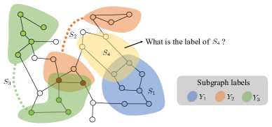
Figure 1. An example of subgraph prediction in base graph $\mathcal{G}$. $\mathcal{S}$ is the set of subgraphs, $\mathcal{S}=\{S_{1},S_{2},S_{3},S_{4}\}$, different colors represent different subgraphs. $S_{2}$ and $S_{3}$ have multiple isolated components, $S_{1}$ has only one component. $S_{2}$ and $S_{3}$ have shared nodes. $\mathcal{Y}$ is the set of labels, $\mathcal{Y}=\{Y_{1},Y_{2},Y_{3}\}$. The task is to predict the label of $S_{4}$.

Subgraph prediction itself is a difficult task because subgraphs are very challenging structures from a topological point of view (Alsentzer et al., 2020). It is necessary to capture the position of all the nodes in the base graph, carry out message passing from nodes inside and outside the subgraph, and consider the dependence of shared edges and nodes in different subgraphs to make the joint prediction. New challenges arise when subgraph prediction meets “small” labeled data: 1) How to learn position encoding for nodes in a simple and effective way? Currently, with limited research on node position encoding, the Position-ware Graph Neural Network (P-GNN) (You et al., 2019) is a feasible solution for node position encoding in subgraph neural networks (Alsentzer et al., 2020). Nevertheless, P-GNN relies on anchors. P-GNN randomly selects nodes on the graph as anchors, then calculates the distance between the target node and anchor nodes, and finally learns the nonlinear distance weighted aggregation on anchors. The overall computational complexity of P-GNN is high. 2) How to automatically augment “good” subgraphs? Data augmentation and self-supervised learning are the main ways to solve GEL. The key criterion for data augmentation is to selectively prevent information loss (Xiao et al., 2021). Existing graph augmentation methods are mainly based on random perturbation (You et al., 2020), sampling (Qiu et al., 2020), or adaptive selection (Zhu et al., 2021; You et al., 2021) on nodes and edges. These methods are unsuitable for subgraph augmentation because a subgraph itself contains fewer nodes, richer structural information, and is more susceptible to undesirable perturbations. 3) Subgraph GEL faces the “bias” problem. We provide statistics of the node coverage in labeled subgraphs of three real-world subgraph datasets: HPO-METAB, EM-USER, and HPO-NEURO. We find that only a small number of nodes in the base graph are contained in the labeled subgraphs, and the coverage are 17.47%, 12.41% and 23.74%, respectively. Details can be found in Table 1 of Section 4.1. Note that shared nodes among subgraphs are not yet counted. This leads to the “bias” problem which means a small number of nodes dominate the subgraph representation learning. Nodes contained in subgraphs are well trained, while nodes not included in subgraphs fail to be fully learned, resulting in the “richer get richer” Matthew effect (Chen et al., 2020). It is a big challenge to the generalization ability of the subgraph prediction problem.

To address the above challenges, in this paper, we propose a Position-Aware Data-Efficient Learning (PADEL) framework for subgraph neural networks. We design a new position encoding scheme that extends cosine position encoding to Non-Euclidean space to assign a hard phase encoding to each node in the base graph. We apply a random 1-hop breadth-first search to diffuse subgraphs and utilize a variational subgraph autoencoder for data augmentation. We develop exploratory and exploitable views for subgraph contrastive learning. The exploratory view encourages subgraphs to explore unseen nodes in the base graph, and the exploitable view selects internal node connections of the subgraph. After a structure-aware pooling with bidirectional LSTM (Graves et al., 2005), the classifier makes the subgraph prediction. The main contributions of this paper are as follows:

• We propose a novel cosine phase position encoding scheme. Our proposed method is anchor-free and is capable of learning an expressive position encoding for each node in the base graph. Compared with existing methods, the computational complexity of our method is reduced.

• We propose a new data augmentation and contrastive learning paradigm for data-efficient subgraph representation learning, which alleviates the bias problem in subgraph GEL.

• We conduct extensive experiments on several datasets, and the results show that our proposed method achieves improvements over state-of-the-art methods.

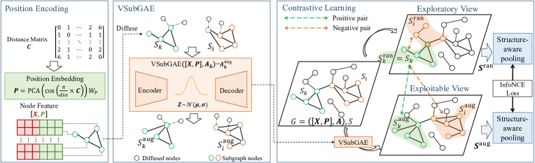
Figure 2. The overall architecture and training pipeline of PADEL. $\boldsymbol{C}$ is the symmetric matrix consisting of distance between nodes. $\boldsymbol{P}$ is the position encoding matrix. $\boldsymbol{X}$ is the node embedding matrix. $\boldsymbol{X}$ and $\boldsymbol{P}$ are concatenated to represent nodes’ feature. We apply a random 1-hop diffusion for each subgraph and feed it into a variational subgraph autoencoder (VSubGAE) to generate augmented subgraphs. We design exploratory and exploitable views for subgraph contrastive Learning. After a structure-aware pooling, we use the InfoNCE loss for training.

2. Related Work

Subgraph Neural Networks

Conventional graph neural networks such as GCN (Kipf and Welling, 2017), GAT (Velickovic et al., 2018), and GIN (Xu et al., 2019) learn node-level or graph-level representations, ignoring the substructures of graphs. Some recent works note this limitation and propose some improvements. For example, selecting and extracting subgraphs for graph pooling (Sun et al., 2021), identifying important subgraphs to explain graph neural network (Yuan et al., 2021), fusing subgraph hierarchical features for link prediction (Liu et al., 2020), classifying subgraphs for link prediction (Lai et al., 2021), and incorporating subgraphs for reasoning (Teru et al., 2020) and link prediction (Joshi and Urbani, 2020) on knowledge graphs. These efforts focus on exploring and utilizing subgraphs for analysis and inference. However, few studies have paid attention to constructing subgraph neural networks for subgraph prediction (i.e., subgraph classification). SPNN (Meng et al., 2018) learns dependent subgraph patterns for subgraph evolution prediction. SubGNN (Alsentzer et al., 2020) is the firstly proposed subgraph neural network that propagates neural messages inside and outside subgraphs in three components: position, neighborhood, and structure. SubGNN follows the position encoding method of P-GNN (You et al., 2019) to select anchors on the base graph randomly. Recently, GLASS (Wang and Zhang, 2022) proposes the max-zero-one labeling trick on SubGNN to learn enhanced subgraph representations. Due to the high computational complexity of SubGNN-related methods, they are not suitable for data-efficient learning.

Self-supervised Learning for GEL

Self-supervised learning for GEL covers node-level GEL, edge-level GEL, and graph-level GEL. For node-level GEL, DGI (Velickovic et al., 2019) and MVGRL (Hassani and Ahmadi, 2020) introduce a discriminator and utilize the global-local contrasting mode. GCA (Zhu et al., 2021) proposes an adaptive augmentation framework with intra and inter contrastive views. For edge-level GEL, SSAL (Hwang et al., 2020) is a self-supervised auxiliary learning method with meta-paths on heterogeneous graphs. SLiCE (Wang et al., 2021a) incorporates global information and learns contextual node representation. For graph-level GEL, GCC (Qiu et al., 2020) and GraphCL (You et al., 2020) are representative graph contrastive learning methods. CCSL (Zeng and Xie, 2021) uses unlabeled graphs to pretrain graph encoders and employs a regularizer for data-efficient supervised classification. GROVER (Rong et al., 2020) designs a transformer-style architecture for learning structural information on unlabeled molecular data. JOAO (You et al., 2021) proposes an automatic and adaptive data augmentation framework under a bi-level min-max optimization. InfoGraph (Sun et al., 2020) proposes to encode aspects of data by using different scales of substructures and contrast them with graph-level representations. GraphLoG (Xu et al., 2021) proposes a base-graph representation learning framework that unifies local instance and global semantic structures. To the best of our knowledge, the study of subgraph-level GEL is still blank.

3. Methodology

The overall architecture of our proposed model conforms to the generic self-supervised training paradigm (Xie et al., 2021). PADEL contains components of position encoding, data augmentation, contrastive learning, and pooling. Figure 2 illustrates the pipeline of PADEL. The downstream task is subgraph prediction which is formulated as follows: $\mathcal{G}=(V,E)$ denotes the base graph, $V$ denotes the node set and $E$ denotes the edge set. $|V|$ and $|E|$ denote the number of nodes and the number of edges, respectively. We focus on undirected graphs. Denote $S_{k}=(V^{\prime}_{k},E^{\prime}_{k})$ as the $k$-th subgraph of $\mathcal{G}$ if $V_{k}^{\prime}\subseteq V$ and $E_{k}^{\prime}\subseteq E$. Each subgraph $S_{k}$ has the corresponding label $Y_{k}$. A subgraph may compromise multiple isolated components or a single component containing some connected nodes. Given a new subgraph $\hat{S}$ in $\mathcal{G}$, we predict the label of $\hat{S}$.

3.1. Cosine Phase Position Encoding

Representing the non-trivial position information for Non-Euclidean structured data (i.e., nodes or subgraphs in the base graph) is still a challenging problem. The Position-aware Graph Neural Network (P-GNN) (You et al., 2019) tackles this problem via randomly selecting nodes as anchors and aggregating anchors’ information to the target node as position encoding. According to the Bourgain theorem (Bourgain, 1985), a graph with $|V|$ nodes requires at least $O(\log^{2}|V|)$ anchors to guarantee the expressiveness of position encoding. SubGNN (Alsentzer et al., 2020) inherits the position encoding method of P-GNN. An obvious limitation is the high computational complexity. In each training iteration in SubGNN, it is necessary to re-select anchors randomly, calculate the shortest path from all nodes to anchors and then aggregate anchors’ information. Besides, a large space complexity with $O(|V|^{2})$ is needed to store the matrix consisting of the shortest paths between nodes in each iteration. The total complexity is very high.

Another limitation of P-GNN is the expressiveness. The propagation of position information in P-GNN is affected by the distance between target nodes and anchors. The aggregated information will be attenuated if the distance is large; therefore, nodes located in the center of the base graph are easy to obtain strong position signals, while nodes located at the edges of the base graph obtain weak position signals. We argue that the above two limitations impede P-GNN for subgraph position encoding.

To solve the problem, we propose our key insight that nodes’ position information in the base graph is innate and can be represented by measuring the distance to other nodes. Inspired by the sequential position encoding method in Transformer (Vaswani et al., 2017) and the Distance Encoding Neural Network (DENN) (Li et al., 2020), we extend the cosine position encoding to Non-Euclidean space to assign a distinctive position encoding for each node in the base graph.

First, we introduce the concept of “diameter” to describe the farthest distance of a node to its reachable nodes. For the base graph $\mathcal{G}=(V,E)$, let $\boldsymbol{C}$ denote the $|V|\times|V|$ symmetric matrix consisting of distances between nodes in $\mathcal{G}$. For example, $\boldsymbol{C}_{i,j}=\boldsymbol{C}_{j,i}$ denotes the distance (i.e., the length of the shortest path obtained by Dijkstra’s algorithm (Dijkstra, 1959)) between nodes $V_{i}$ and $V_{j}$. The diagonal elements of $\boldsymbol{C}$ are all 0, i.e., $\boldsymbol{C}_{i,i}=0$. If node $V_{i}$ cannot reach $V_{j}$, $\boldsymbol{C}_{i,j}=\boldsymbol{C}_{j,i}=\infty$. We use $dia_{i}$ to represent the “diameter” of the $i$-th node $V_{i}$,

(1) $$dia_{i}=\max_{j}\boldsymbol{C}_{i,j},\quad\text{where }\boldsymbol{C}_{i,j}\neq\infty,$$

$dia_{i}$ is the maximum value of the shortest path length from $V_{i}$ to all reachable nodes.

Then, we propose to use the cosine function to encode the matrix $\boldsymbol{C}$. Since the value of $dia_{i}$ could be very large when there are many nodes in graph $\mathcal{G}$, $dia_{i}$ will fluctuate widely in value. Utilizing the periodic property of the cosine function, we apply the function of Eq.(2) to obtain a scaled matrix $\hat{\boldsymbol{C}}$:

(2) $$\hat{\boldsymbol{C}}_{i,j}=\left\{\begin{aligned} &\cos(\frac{\pi}{dia_{i}}\times\boldsymbol{C}_{i,j})&,&\boldsymbol{C}_{i,j}\neq\infty\\ &-1.5&,&\boldsymbol{C}_{i,j}=\infty,\end{aligned}\right.$$

where $\cos(\frac{\pi}{dia_{i}}\times\boldsymbol{C}_{i,j})$ means for each node $v_{i}$, its all reachable nodes $v_{j}$ (including $v_{i}$ itself) are mapped to phase $[0,\pi]$. In other words, among all reachable nodes, the distance of the node closest to $v_{i}$ (itself) is mapped to 1. The distance of other reachable nodes is mapped to smaller values, and if the distance is farther, the mapped value is closer to -1. Unreachable nodes are mapped to a smaller number than -1 (e.g., -1.5). If we think of each element $\boldsymbol{C}_{i,j}$ in $\boldsymbol{C}_{i}$ as a discrete phase value of the cosine function, $\boldsymbol{C}_{i}$ can be viewed as the superposition of different cosine phase values. The processed matrix $\hat{\boldsymbol{C}}$ has the following properties:

• Normalization: The computed phases $\frac{\pi}{dia_{i}}\times\boldsymbol{C}_{i,j}$ in Eq. (2) range in $[0,\pi]$, so $\hat{\boldsymbol{C}}_{i,j}\in[-1,1]$ for reachable nodes, and -1.5 for the others.

• Distinctiveness: Each row in $\hat{\boldsymbol{C}}$ is distinguished from others, because $\boldsymbol{C}$ is symmetric and $\hat{\boldsymbol{C}}_{ii}=1$.

• Interpretability: Each element in $\hat{\boldsymbol{C}}_{i}$ is closely related to the minimal number of hops between node $i$ and all nodes.

Next, we employ the Principal Component Analysis (PCA) (Wold et al., 1987) to reduce the dimension of $\hat{\boldsymbol{C}}$ to the size of $|V|\times d^{\prime}$, where $d^{\prime}$ is a manually set hyperparameter,

(3) $$\overline{\boldsymbol{C}}=\text{PCA}(\hat{\boldsymbol{C}}).$$

Last, we perform a linear projection on $\overline{\boldsymbol{C}}$ to generate the position embedding matrix $\boldsymbol{P}$ with the size of $|V|\times d$,

(4) $$\boldsymbol{P}=\overline{\boldsymbol{C}}\boldsymbol{W}_{P},$$

where $\boldsymbol{W}_{P}\in\mathbb{R}^{d^{\prime}\times d}$ is a learnable parameter matrix. The reason we introduce the projection matrix $P$ is to make position encoding scalable. Since we need to manually specify the dimension for PCA, it’s not flexible if we want to adjust the dimension of position encoding. If we apply the projection matrix $\boldsymbol{W}_{P}$ directly to $\hat{\boldsymbol{C}}$, $\boldsymbol{W}_{P}$ will be large, and more importantly, it brings instability to the subsequent training of the model (i.e., the KL term in Eq. (9) will be extremely large).

Compared with P-GNN, our proposed cosine phase position encoding has the following advantages: 1) Our method is anchor-free. The position information is measured only by distance between nodes. 2) The Cosine phase position encoding matrix $\hat{\boldsymbol{C}}$ has the nature of normalization, distinctiveness, and interpretability as analyzed above. 3) Our position encoding method is expressive. We provide a case study in section 4.5 (See Fig. 5). The above three advantages make our method not only a general-purpose position encoding method but also suitable for data-efficient subgraph neural networks.

3.2. Variational SubGraph AutoEncoder for Data Augmentation

It is essential to prevent information loss during data augmentation (Xiao et al., 2021). The quality of an augmented graph is crucial in graph contrastive learning (You et al., 2021). Existing methods (You et al., 2020; Qiu et al., 2020; Zhu et al., 2021; You et al., 2021) are not suitable for subgraph augmentation because a subgraph contains only a small part of the nodes in the base graph, but contains rich position and structural information, which needs to be augmented with appropriate strategies. Unlike existing graph augmentation methods, we utilize generative models to augment subgraphs in PADEL. Specifically, we design a Variational SubGraph AutoEncoder (VSubGAE) with random 1-hop node diffusion.

Given the base graph $\mathcal{G}$ with $|V|$ nodes, suppose the node embedding matrix is $\boldsymbol{X}\in\mathbb{R}^{|V|\times d}$. We assign a unique feature vector to each node since some nodes may be shared in different subgraphs, and some nodes may not appear in any subgraph. For the $k$-th subgraph $\boldsymbol{S}_{k}$, its corresponding adjacency matrix is $\boldsymbol{A}_{k}$.

The Encoder.

For the $i$-th node $v_{i}\in S_{k}$, we have the corresponding node feature vector $\boldsymbol{x}_{i}$ and the position encoding $\boldsymbol{p}_{i}$. We concatenate $\boldsymbol{x}_{i}$ and $\boldsymbol{p}_{i}$, and feed them into the encoder of VSubGAE which is a two-layer GCN:

(5) $$q(\boldsymbol{z}_{k,i}|[\boldsymbol{X},\boldsymbol{P}],\boldsymbol{A}_{k})\sim\mathcal{N}(\boldsymbol{\mu}_{i}([\boldsymbol{X},\boldsymbol{P}],\boldsymbol{A}_{k}),\boldsymbol{\sigma}_{i}([\boldsymbol{X},\boldsymbol{P}],\boldsymbol{A}_{k})),$$

where $[\cdot,\cdot]$ denotes concatenation, $\mathcal{N}(\cdot,\cdot)$ denotes the Gaussian distribution. $\boldsymbol{\mu}=\mathrm{GCN}_{\mu}([\boldsymbol{X},\boldsymbol{P}],\boldsymbol{A}_{k})$ and $\boldsymbol{\sigma}=\mathrm{GCN}_{\sigma}([\boldsymbol{X},\boldsymbol{P}],\boldsymbol{A}_{k})$. $\mathrm{GCN}_{\mu}$ and $\mathrm{GCN}_{\sigma}$ are defined as:

(6) $$\mathrm{GCN_{\mu,\sigma}}([\boldsymbol{X},\boldsymbol{P}],\boldsymbol{A}_{k})=\boldsymbol{\tilde{A}}_{k}\mathrm{ReLU}(\boldsymbol{\tilde{A}}_{k}[\boldsymbol{X}_{v\in V_{k}},\boldsymbol{P}_{v\in V_{k}}]\boldsymbol{W}_{1})\boldsymbol{W}_{\mu,\sigma},$$

where $\boldsymbol{\tilde{A}}_{k}=\boldsymbol{D}_{k}^{-\frac{1}{2}}\boldsymbol{A}_{k}\boldsymbol{D}_{k}^{-\frac{1}{2}}$ and $\boldsymbol{D}_{k}$ is the degree matrix of $S_{k}$. $\boldsymbol{W}_{1}\in\mathbb{R}^{2d\times 2d}$ is the shared learnable matrix, $\boldsymbol{W}_{\mu},\boldsymbol{W}_{\sigma}\in\mathbb{R}^{2d\times 2d}$ are learnable matrices. The parameters of GCN layers are shared among all of the subgraphs. The inference process is defined as:

(7) $$q(\boldsymbol{Z}|[\boldsymbol{X},\boldsymbol{P}],\mathcal{A})=\prod_{k=1}^{K}\prod_{i=1}^{|V^{\prime}_{k}|}q(\boldsymbol{z}_{k,i}|[\boldsymbol{X},\boldsymbol{P}],\boldsymbol{A}_{k}),$$

where $\mathcal{A}=\{\boldsymbol{A}_{1},\boldsymbol{A}_{2},\cdots,\boldsymbol{A}_{K}\}$ is the collection of adjacency matrices with $K$ elements. The reparameterization trick is used to sample a node feature: $\boldsymbol{z}_{k,i}=\boldsymbol{\mu}_{i}([\boldsymbol{X},\boldsymbol{P}],\boldsymbol{A}_{k})+\boldsymbol{\sigma}_{i}([\boldsymbol{X},\boldsymbol{P}],\boldsymbol{A}_{k})\odot\boldsymbol{\epsilon}$, where $\odot$ represents point-wise product between two vectors, $\boldsymbol{\epsilon}\sim\mathcal{N}(0,\boldsymbol{I}_{k})$.

The decoder.

We use a simple inner product between latent variables as the decoder, which obtains the possibility of two edges connecting to each other. Thus we have:

(8) $$p(\mathcal{A}|\boldsymbol{Z}) =\prod_{k=1}^{K}\prod_{i=1}^{|V_{k}^{\prime}|}\prod_{j=1}^{|V_{k}^{\prime}|}p(A_{k,ij}|\boldsymbol{z}_{k,i},\boldsymbol{z}_{k,j})$$

$$=\prod_{k=1}^{K}\prod_{i=1}^{|V_{k}^{\prime}|}\prod_{j=1}^{|V_{k}^{\prime}|}\mathrm{Sig}(\boldsymbol{z}_{k,i}\boldsymbol{z}_{k,j}),$$

where $\mathrm{Sig}(\cdot)$ denotes the Sigmoid function.

VSubGAE Optimization.

Following VGAE (Kipf and Welling, 2016) and $\beta$-VAE (Higgins et al., 2017), the optimization goal of VSubGAE is to maximize the variational Evidence Lower Bound (ELBO) with coefficient $\beta$ , which balances the reconstruction accuracy of subgraphs with the independence constraints of the latent variables (i.e. the KL divergence term in $\mathcal{L}_{VSubGAE}$):

(9) $$\mathcal{L}_{VSubGAE}= \mathbb{E}_{\boldsymbol{Z}\sim q(\boldsymbol{Z}|[\boldsymbol{X},\boldsymbol{P}],\mathcal{A})}\log{p(\mathcal{A}|\boldsymbol{Z})}$$

$$-\beta\cdot\mathrm{KL}(q(\boldsymbol{Z}|[\boldsymbol{X},\boldsymbol{P}],\mathcal{A})||p(\boldsymbol{Z})),$$

where $p(\boldsymbol{Z})\sim\mathcal{N}(0,\boldsymbol{I})$ is the prior distribution of latent variables $\boldsymbol{Z}$, following the common practice in (Higgins et al., 2017; Kipf and Welling, 2016).

3.3. Contrastive Learning in PADEL

We train PADEL in a self-supervised manner by contrasting positive and negative sample pairs. As we analyzed in section 1, nodes in subgraphs are only a small part of the base graph. This results in a bias problem which means “hot” nodes (contained in subgraphs) will dominate model training, and “long-tail” nodes (not included in subgraphs) fail to be fully learned. Although we alleviate the problem to some extent by using 1-hop diffusion in the VSubGAE component, nodes far from subgraphs are still unexplored. To further alleviate the bias problem, we propose Exploratory and Exploitable views for subgraph contrastive learning, which is the right part in Figure 2.

The Exploratory View

We design an exploratory view (abbreviated as Explore-View) for data augmentation to enable our model to explore unseen nodes in the base graph. We randomly sample subgraphs in $\mathcal{G}$ as augmented data, which allows our model to explore more distant undetected nodes. Let the $k$-th subgraph be the positive sample, we generate exploratory subgraphs $\mathcal{S}^{\text{ran}}$ by:

(10) $$S^{\text{ran}}_{i}=\left\{\begin{aligned} &S_{k},&\text{if }i=k,\\ &\text{RandomWalk}(hop),&\text{otherwise},\end{aligned}\right.$$

where $\text{RandomWalk}(hop)$ means performing $hop$-step random walks on the base graph to generate a random subgraph. $hop$ is equal to the average number of nodes for a given dataset.

The Exploitable View

In addition to exploring distant nodes in the base graph, we also need to find the appropriate perturbation from the subgraph for augmentation adaptively. We consider this an exploitable view (abbreviated as Exploit-View) that changes a subgraph’s internal connections. To augment data adaptively, we use VSubGAE to generate the augmented adjacency matrix $A_{k}^{aug}$ for subgraph $S_{k}^{aug}$ by Eq. (7) and (8), which can be denoted as:

(11) $$\boldsymbol{S}_{k}^{aug}\leftarrow\boldsymbol{A}^{\text{aug}}_{k}=\text{VSubGAE}([\boldsymbol{X},\boldsymbol{P}],\boldsymbol{A}_{k}).$$

Contrastive Learning

Given the subgraph set $\mathcal{S}$ containing $K$ subgraphs, we train all $K$ subgraphs in one training step. Each subgraph is treated as a positive sample, while others are treated as negative ones. Exploratory subgraphs are sampled for each positive sample separately in each training step.

The Exploratory view augmentation and Exploitable view augmentation generate augmented subgraphs $\mathcal{S}^{\text{ran}}$ and $\mathcal{S}^{\text{aug}}$, respectively. For the $k$-th subgraph, we choose the exploratory view $\boldsymbol{S}^{\text{ran}}_{k}$ and the exploitable view $\boldsymbol{S}^{\text{aug}}_{k}$ as the positive pair. We define positive and negative pairs as follows:

• Positive pair: $(S^{\text{ran}}_{k},S^{\text{aug}}_{k})$.

• Explore-View negative pairs: $\{(S^{\text{ran}}_{k},S^{\text{ran}}_{i})$, where $i\neq k\}$.

• Exploit-View negative pairs: $\{(S^{\text{ran}}_{k},S^{\text{aug}}_{i})$, where $i\neq k\}$.

The InfoNCE loss is computed as follows:

(12) $$\mathcal{L}_{\text{InfoNCE}}(k,\boldsymbol{E}^{\text{ran}},\boldsymbol{E}^{\text{aug}})=$$

$$-\log\frac{e^{\theta\left(S^{\text{ran}}_{k},S^{\text{aug}}_{k}\right)}}{\underbrace{e^{\theta\left(S^{\text{ran}}_{k},S^{\text{aug}}_{k}\right)}}_{\text{Positive Pair }}+\underbrace{\sum_{i\neq k}e^{\theta\left(S^{\text{ran}}_{k},S^{\text{ran}}_{i}\right)}}_{\text{Explore-View negative pairs }}+\underbrace{\sum_{i\neq k}e^{\theta\left(S^{\text{ran}}_{i},S^{\text{aug}}_{k}\right)}}_{\text{Exploit-View negative pairs }}},$$

where $\theta$ is the contrastive score as the sum of cosine similarity for both neighbor-position encoding $\boldsymbol{E}^{\text{NP}}$ and structure-position encoding $\boldsymbol{E}^{\text{S}}$ (See section 3.4):

(13) $$\theta(S_{i},S_{j})=\frac{\left<\boldsymbol{E}^{\text{NP}}_{i},\boldsymbol{E}^{\text{NP}}_{j}\right>}{||\boldsymbol{E}^{\text{NP}}_{i}||\times||\boldsymbol{E}^{\text{NP}}_{j}||}+\frac{\left<\boldsymbol{E}^{\text{S}}_{i},\boldsymbol{E}^{\text{S}}_{j}\right>}{||\boldsymbol{E}^{\text{S}}_{i}||\times||\boldsymbol{E}^{\text{S}}_{j}||},$$

where $\left<\cdot,\cdot\right>$ denotes inner product and $||\cdot||$ denotes the norm.

Next section will discuss how to compute subgraph encoding $\boldsymbol{E}^{\text{NP}},\boldsymbol{E}^{\text{S}}$ with our structure-aware subgraph pooling model.

3.4. Structure-Aware Subgraph Pooling

Graph readout plays an important role in GEL (Mesquita et al., 2020). We develop a structure-aware subgraph pooling method. The pooling architecture is shown in Figure 3. Our pooling component is designed to learn structure-aware subgraph representations that can capture three aspects of information: neighborhood, position, and structure. The inputs are node embedding matrix $\boldsymbol{X}$ and position encoding matrix $\boldsymbol{P}$. We implement structure-aware subgraph pooling through neighbor nodes’ message passing with position information and structure extraction based on the position information.

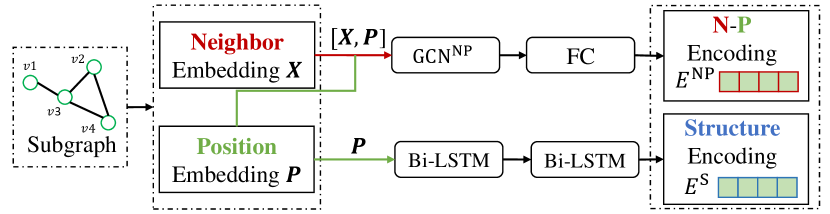
Figure 3. The structure-aware subgraph pooling component. The lower part illustrates how Bi-LSTM layers extract structure encoding $E^{NP}$ of a given subgraph.

Neighbor Aggregation with Position Information

Node embedding and position encoding of subgraph $S_{k}$ are concatenated as the input of a GCN layer, and then through a fully-connected layer followed by an average pooling layer:

(14) $$\boldsymbol{E}_{k}^{\text{NP}}=avg\_pool(\text{ReLU}(\text{GCN}^{\text{NP}}([\boldsymbol{X},\boldsymbol{P}],\boldsymbol{A}_{k})\boldsymbol{W}^{\text{FC}})),$$

where $[\cdot,\cdot]$ denotes concatenation, $\boldsymbol{A}_{k}$ is the adjacency matrix of the input subgraph $\boldsymbol{S}_{k}$, $\boldsymbol{W}^{\text{FC}}\in\mathbb{R}^{2d\times\hat{d}}$ is the learnable parameter matrix.

Structure Extraction with Position Information

We believe that the structural information in the graph should be innate and task-agnostic. In subgraphs, the encoded position encoding matrix $\boldsymbol{P}$ is considered as the prior information describing each node’s position in the base graph. Naturally, we extract the subgraph’s structural feature denoted as $\boldsymbol{E}^{\text{S}}$ from its nodes’ position information. We adopt a two-layer Bi-LSTM (Graves et al., 2005) as the extractor. Since Bi-LSTM is capable of learning order-invariant information, it is useful to extract the subgraph’s structural information (Alsentzer et al., 2020). Nodes in the subgraph are reorganized into a sequence and fed into the Bi-LSTM unit. We use the hidden state of the last Bi-LSTM layer as the structure encoding:

(15) $$\boldsymbol{E}_{k}^{\text{S}}=\text{ReLU}(\text{Bi-LSTM}(\boldsymbol{P}_{v\in V_{k}})).$$

We also tried different kinds of layers, such as attention layers and one Bi-LSTM layer; we found that using two Bi-LSTM layers is the best choice.

3.5. Objective Functions and Optimization

For subgraph encoding $\boldsymbol{E}=\{\boldsymbol{E}^{\text{NP}},\boldsymbol{E}^{\text{S}}\}$, we use a 1-layer fully-connected networks to compute classification logits $\hat{\boldsymbol{Y}}$ as follows:

(16) $$\hat{\boldsymbol{Y}}=(\boldsymbol{E}^{\text{NP}}+\boldsymbol{E}^{\text{S}})\boldsymbol{W}^{\text{S}},$$

where $\boldsymbol{W}^{\text{S}}\in\mathbb{R}^{\hat{d}\times l}$ is the parameter matrix, $l$ depends on the downstream task. $\hat{\boldsymbol{Y}}$ is a vector with the same number of elements as the total class number. Let $Y$ denote the one-hot vector of the ground-truth label, we use the Cross-Entropy Loss $\mathcal{L}_{\text{CE}}$ as follows:

(17) $$\mathcal{L}_{\text{CE}}(Y,\hat{\boldsymbol{Y}})=-\sum_{i}Y_{i}\log\frac{exp^{\hat{Y}_{i}}}{\sum_{j}exp^{\hat{Y}_{j}}}.$$

4. Experiments

We provide the pseudocode of the algorithm of VSubGAE’s random 1-hop subgraph diffusion, the training pipeline of PADEL, and the training data in our anonymous external repository.

4.1. Datasets

Table 1. Statistics of Datasets.

Dataset	#Nodes	#Edges	#Subgraphs	#Nodes in Subgraphs	Coverage	Multi-Label
HPO-METAB	14587	3238174	2400	2548	17.47%
EM-USER	57333	4573417	324	7115	12.41%
HPO-NEURO	14587	3238174	4000	3463	23.74%	Y

To evaluate the effectiveness of our proposed method PADEL, we conduct extensive experiments on three real-world datasets: HPO-METAB, EM-USER, and HPO-NEURO. All three datasets are released in (Alsentzer et al., 2020) by the Harvard team and are used in the source code of SubGNN . Table 1 describes their statistics.

• HPO-METAB is a dataset of clinical diagnostic task for rare metabolic disorders. The base graph contains information on phenotypes and genotypes of rare diseases, in which the nodes denote the genetic phenotypes of the diseases and the edges represent the relationships between phenotypes. Information on relationships is obtained from the Human Phenotype Ontology (HPO) (et al., 2019b) and rare disease diagnostic data (Austin and Dawkins, 2017; Kim and Price, 2011; Hartley et al., 2020). Each subgraph consists of a set of phenotypes associated with rare monogenic metabolic diseases, with a total of 6 metabolic diseases. Subgraph labels represent the diagnosis categories.

• HPO-NEURO is used to diagnose rare neurological diseases. It shares the same base graph with HPO-METAB but has different subgraphs. Each subgraph has multiple disease category labels and contains 10 neurological disease categories.

• EM-USER’s base graph is from the Endomondo (Ni et al., 2019) social fitness network used to analyze user properties, where nodes represent exercises, and edges will exist if users finish exercises. Subgraphs show the user’s exercise records, while labels represent the 2 genders of the user.

4.2. Experimental settings

Data Processing.

Following SubGNN (Alsentzer et al., 2020), for HPO-METAB and HPO-NEURO datasets, we randomly divide 80% of the data into the training set, 10% of the data into the validation set, and 10% of the data into the test set. For the EM-USER dataset, the proportions are 70%, 15%, and 15%, respectively. Since our model is for data-efficient learning, we randomly select 10% of the original training set as our data-efficient training set. All methods are trained with the same data-efficient training set. The validation and test sets remain the same with the original dataset.

Baselines

We compare the performance of PADEL with the following baseline methods. GCN (Kipf and Welling, 2017) is the conventional graph convolutional network (Kipf and Welling, 2017). GAT (Velickovic et al., 2018) is the graph neural network with attention mechanism. GIN (Xu et al., 2019) is the graph isomorphism network with powerful representation learning capabilities. GraphCL (You et al., 2020) is the representative graph contrastive learning method. GCA (Zhu et al., 2021) is a node-level graph contrastive learning method with adaptive augmentation. JOAO (You et al., 2021) is the automated graph augmentation method which augments graphs adaptively, automatically and dynamically. SubGNN (Alsentzer et al., 2020) and GLASS (Wang and Zhang, 2022) are the state-of-the-art (SOTA) subgraph neural networks.

Evaluation Protocals

We adopt the Micro F1 Score(Alsentzer et al., 2020) as the evaluation metric. Higher scores indicate better performance.

Reproducibility Settings

We develop our model with PyTorch (et al., 2019a) and NetworkX (Hagberg et al., 2008). All methods are trained on a single GeForce RTX 2080Ti GPU. We repeat the experiment 10 times for all methods, each time with a different random seed. After ten experiments, we record the mean and standard deviation of the results. For a fair comparison, the input dimension for all methods is set to 64. In our model, the dimension of the node feature is set to 32, and the dimension of position embedding is also set to 32, so the total dimension is 64. We set the batch size to 32 and set the maximal training epoch to 3000 for all methods to ensure training convergence. We use the AdamW (Loshchilov and Hutter, 2019) optimizer for optimization and set the weight decay to 1e-2 in AdamW. We search the learning rate in the range of {1e-3, 5e-3, 1e-2} for all methods. The coefficient $\beta$ in VSubGAE is set to 0.2 according to beta-VAE (Higgins et al., 2017).

For GCN and GAT, we use a default 3-layer graph neural network. For GIN, we use a default 3-layer perceptron. For GraphCL (You et al., 2020) and JOAO (You et al., 2021), we convert test datasets to the TUDataset format while retaining all subgraph internal edges and subgraph labels, and we use the default semi-supervised learning setup (the scaling parameter is set to 4 for HPO-METAB and HPO-NEURO datasets, and 5 for the EM-USER dataset). Since GCA (Zhu et al., 2021) is for node classification, we extend it to the subgraph classification task by adding an average pooling layer. For SubGNN (Alsentzer et al., 2020), we use the optimal model hyperparameters suggested in the official source code .

For multi-label classification on the HPO-NEURO dataset, we treat it as a multiple binary classification task. We calculate the accumulated loss on each label position by using the Binary Cross Entropy loss:

(18) $$\mathcal{L}_{\text{BCE}}=-\sum_{i}[Y_{i}\log({\text{Sig}(\hat{Y}_{i})})+(1-Y_{i})\log(1-\text{Sig}(\hat{Y}_{i}))],$$

where Sig denotes the Sigmoid function.

Table 2. Performance on GEL on 10% original training set (the best in bold). Underline denotes the best baseline.

Method	HPO-METAB (10%)	EM-USER (10%)	HPO-NEURO (10%)
GCN	24.43±1.61	48.37±0.93	44.84±1.04
GAT	27.06±3.50	51.63±5.58	36.82±2.71
GIN	11.91±9.89	45.58±6.34	33.24±6.60
GraphCL	24.00±0.38	55.17±2.32	32.01±0.36
GCA	35.32±3.47	58.18±6.46	48.28±1.72
JOAO	24.16±0.40	54.83±1.22	32.45±0.35
SubGNN	37.87±4.02	58.78±6.63	51.36±2.09
GLASS	31.58±6.67	53.46±5.06	47.68±4.19
Our Method	44.72±1.34	68.45±5.51	53.33±0.75
Improvement (%)	18.09	16.45	3.84

Table 3. The performances on three datasets with different scales of training data (the best in bold).

	10%	20%	30%	40%	50%	100%
HPO-METAB	37.87±4.02	42.17±3.64	46.51±3.00	48.13±3.71	50.04±2.76	54.72±2.48	SubGNN
	31.58±6.67	44.88±5.14	46.80±4.72	51.64±2.55	57.02±5.26	62.98±3.84	GLASS
	44.72±1.34	49.33±1.47	49.69±1.40	51.64±1.62	55.85±1.66	56.26±0.91	Our Method
EM-USER	58.78±6.63	68.98±4.54	73.27±7.27	80.41±1.00	82.45±1.63	81.43±4.87	SubGNN
	53.46±5.06	57.12±4.65	61.66±8.40	76.74±6.88	82.44±2.08	84.92±3.56	GLASS
	68.45±5.51	73.56±5.30	77.33±3.56	82.00±2.89	84.00±2.95	84.96±3.46	Our Method
HPO-NUERO	51.36±2.09	56.63±1.65	59.07±1.15	60.04±0.93	60.11±1.82	64.20±1.63	SubGNN
	47.68±4.19	53.64±1.41	61.18±2.90	63.20±0.72	64.44±1.48	68.42±0.66	GLASS
	53.33±0.75	58.41±1.35	60.35±1.20	61.09±1.02	62.70±0.87	65.18±1.41	Our Method

4.3. Performance Comparison

Overall Performance.

Table 2 describes the overall performance, we can find the following observations:

• PADEL outperforms all baseline methods on three datasets, and the improvement is achieved. PADEL achieves an average improvement of 12.79% compared with the SOTA method SubGNN.

• Conventional methods GCN, GAT, and GIN don’t perform well. The possible reason is that their representation learning ability decreases sharply in subgraph neural networks.

• Graph augmentation-based methods GraphCL, GCA, and JOAO perform better than conventional methods in general, but the results are subtle. We find that GraphCL and JOAO perform worse on HPO-METAB and HPO-NEURO datasets than GCN and GAT. It reflects the fact that existing graph-level augmentation methods are very limited in subgraph neural networks. GCA performs much better than GraphCL and JOAO on three datasets. The possible reason is that GCA is a node-level self-supervised learning method, it learns node representation effectively by the intra- and inter-view contrastive learning using adaptive augmentation.

• SubGNN achieves the previous SOTA performance. SubGNN is a sophisticated method for extracting subgraph representations and passing messages between subgraphs, and this is the reason why SubGNN performs best of all baseline methods. Our proposed model PADEL outperforms SubGNN by large margins. There are three possible reasons: 1) Nodes’ position information is well captured and learned. 2) The augmentation-contrastive learning paradigm in PADEL is effective. 3) The pooling method in PADEL captures subgraphs’ structures.

Performance on different scales of data.

We compare PADEL with SOTA baselines SubGNN and GLASS by taking 10%, 20%, 30%, 40%, 50%, and 100% of the training set on three datasets to verify their performance. Table 3 describes the results. We have the observation that PADEL outperforms SubGNN across the board. PADEL shows comparative performance with GLASS, but outperforms GLASS in most data-efficient situations.

Time Cost.

To compare the time cost, we test on the HPO-METAB (10%) dataset using a single GPU. SubGNN requires preprocessing of the data file, spending 12 minutes calculating the metric of shortest path length, 4 hours calculating the metric of subgraph similarity, and 12 hours calculating node embedding. The training time of SubGNN is 227 seconds for 100 epochs.

Table 4. The time cost on HPO-METAB (10%) dataset.

	Step	SubGNN	GLASS	PADEL	Speed Up
Pretrain	Metrics	4 h 12 min	0	12 min	46 / 65 $\times$
	Embedding	12 h	23 h	557 sec
Train	Subgraph	227 sec	79 sec	39 sec	6 / 2 $\times$

In the pre-training phase, GLASS doesn’t need to compute metrics, but it need 23 hours to pretrian its node embeddings. The average training time of GLASS is 79 seconds for 100 epochs. In comparison, PADEL spends 12 minutes calculating the shortest path lengths, 17 seconds calculating VSubGAE, and 540 seconds on contrast learning. The training time of PADEL is 39 seconds for 100 epochs. Compared with SuhbGNN, the pretraining time of PADEL is 46 times shorter, and the training time is 6 times shorter. PADEL also takes 65 $\times$ time shorter in pretraining and 2 $\times$ time shorter in training than GLASS. Results are shown in Table 4. We find that the most time-consuming step in PADEL is calculating the distance matrix $\boldsymbol{C}$ for 12 minutes because of the $O(|V|^{3})$ time complexity of the Dijkstra’s algorithm. Although existing SubGNN and its variants (Alsentzer et al., 2020; Wang and Zhang, 2022) also need to pre-compute $\boldsymbol{C}$, we leave the problem of learning position embedding more efficiently and making it suitable for larger-scale graphs in future works.

4.4. Ablation Study

To investigate different components’ effectiveness in PADEL, we design eight cases for ablation study ($C_{0}$-$C_{7}$). $C_{0}$: Only apply the Subgraph Pooling (PL) module. $C_{1}$: Only pre-train the node embedding matrix $\boldsymbol{X}$ using VSubGAE in a Self-Supervised (SS) manner. The position embedding matrix $\boldsymbol{P}$ is initialized randomly. $C_{2}$: Only train the Position Encoding (PE). $C_{3}$: Initialize node embedding matrix $\boldsymbol{X}$ and position embedding matrix $\boldsymbol{P}$ randomly, and train PADEL by Contrastive Learning (CL). The subgraph generator VSubGAE is randomly initialized during training. $C_{4}$: Remove CL, but SS and PE are retained. $C_{5}$: Remove PE, but SS and CL are retained. The outputs of VSubGAE are fed into CL without position embedding. $C_{6}$: Remove SS, use the position embedding matrix $\boldsymbol{P}$ as input features. $C_{7}$: Use all components.

As shown in Table 5, each component of PADEL has a positive impact on results. The combination of all components brings the best results, which is much better than using any component alone. Using two components is better than using a single component, except for $C_{5}$. It indicates that PE contributes the most to the model, as can be seen from the results of $C_{2}$, $C_{4}$, and $C_{6}$. We observe that $C_{1}$ is worse than $C_{0}$ on the EM-USER dataset. We conduct an in-depth investigation and find that the subgraphs in EM-USER dataset are much larger than those in the other two datasets, so VSubGAE will truncate some of the nodes in the input, resulting in a high VSubGAE reconstruction loss.

Table 5. We implement 8 variants of PADEL ($C_{0}$-$C_{7}$). The abbreviations in table: Self-Supervised (SS) learning, Position Encoding (PE), Contrastive Learning (CL), Pooling (PL).

SS	PE	CL	PL		HPO-METAB (10%)	EM-USER (10%)	HPO-NEURO (10%)
			Y	$C_{0}$	31.28±4.11	53.12±8.79	43.67±2.33
Y			Y	$C_{1}$	35.80±2.80	52.00±9.75	45.07±1.09
	Y		Y	$C_{2}$	39.10±3.16	62.67±8.36	49.82±1.05
		Y	Y	$C_{3}$	33.49±2.88	59.11±3.61	47.99±1.28
Y	Y		Y	$C_{4}$	40.21±3.60	63.78±6.21	50.43±1.61
Y		Y	Y	$C_{5}$	38.55±2.13	56.45±5.37	47.15±1.41
	Y	Y	Y	$C_{6}$	42.47±1.88	65.33±5.46	52.04±1.37
Y	Y	Y	Y	$C_{7}$	44.72 ±1.34	68.45±5.51	53.33±0.75

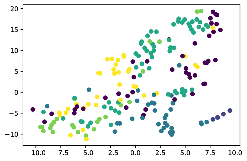
(a) Our Method

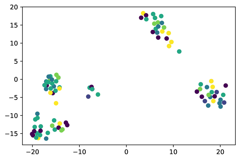
(b) w.o. PE & Contrastive Learning

Figure 4. Comparison of subgraph embeddings. Points in (a) are projections learned by PADEL. Points in (b) are learned without position encoding and contrastive learning.

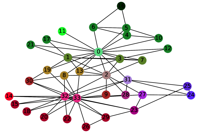
(a) 3D position embedding.

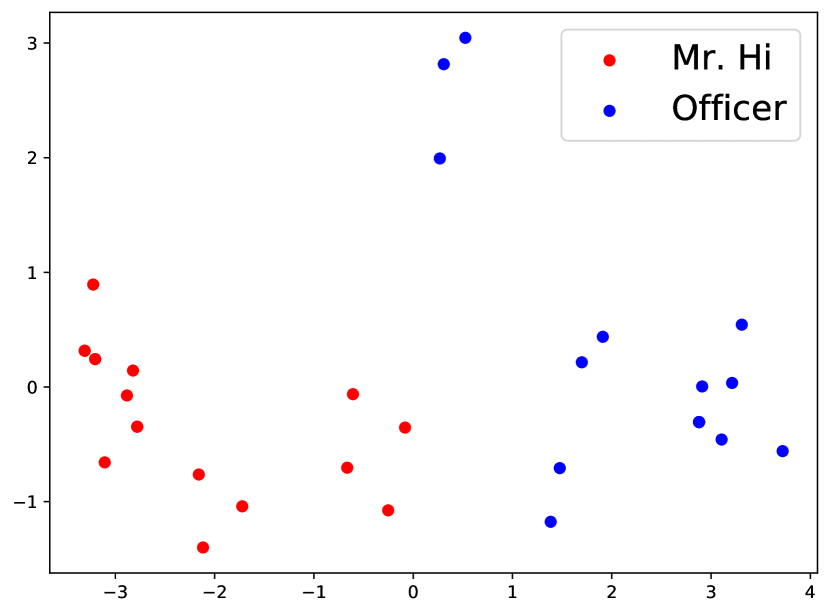
(b) 2D position embedding.

Figure 5. Case study of cosine position encoding $\boldsymbol{P}$. (a) Position encoding as RGB value to color each node. Adjacent nodes have similar colors. (b) The 2-dimensional position embedding for each node. Node color illustrates its label.

4.5. Case Study

This section attempts to understand how PADEL facilitates subgraph representation learning. We select subgraphs in the HPO-METAB dataset, obtain their feature vectors after subgraph pooling, and visualize them via t-SNE (Van der Maaten and Hinton, 2008) projection. Figure 4(a) illustrates the results learned by PADEL, and Figure 4(b) illustrates the results using simple end-to-end training without position encoding and contrastive learning. Each point represents a subgraph, and different colors represent different labels. We can find that subgraphs with the same label are more likely to cluster together in Figure 4(a), whereas subgraphs are entangled and hard to distinguish in Figure 4(b). It indicates that position encoding and contrastive learning help the model learning subgraph representation.

We provide a toy example on the Zachary’s karate club network (Girvan and Newman, 2002) to illustrate the expressiveness of our PE. We apply 3-dimensional cosine position embedding for each node in the graph. We categorize each node’s position encoding as a Red-Green-Blue value and color each node to visualize them. Figure 5(a) illustrates the results. We can observe that nodes close to each other have similar colors. Further, we reduce the dimension to 2 and plot the scatter of $\boldsymbol{P}$. The results are shown in Figure 5(b). The position encoding makes nodes linearly separable without supervised signal.

5. Conclusion

Learning subgraph neural networks given “small” data is a challenging task. This paper proposes a novel position-aware data-efficient subgraph neural networks called PADEL to solve the problem. We develop a novel position encoding method that is simple and powerful, design a generative subgraph augmentation method utilizing a variational subgraph autoencoder with random 1-hop subgraph diffusion, and develop exploratory and exploitable views for subgraph contrastive learning by a structure-aware pooling architecture. The self-supervised paradigm in PADEL helps to alleviate the bias problem in the subgraph prediction problem. Experiments on three real-world datasets show that our PADEL method surpasses the SOTA method by a large margin.

- (1)
- Alsentzer et al. (2020) Emily Alsentzer, Samuel G. Finlayson, Michelle M. Li, and Marinka Zitnik. 2020. Subgraph Neural Networks. In NeurIPS.
- Austin and Dawkins (2017) Chris P. Austin and Hugh J. S. Dawkins. 2017. Medical research: Next decade’s goals for rare diseases. NATURE 548 (2017), 158–158.
- Bourgain (1985) Jean Bourgain. 1985. On Lipschitz embedding of finite metric spaces in Hilbert space. ISR J MATH 52, 1-2 (1985), 46–52.
- Bradley (2020) Conor A Bradley. 2020. A statistical framework for rare disease diagnosis. NAT REV GENET 21, 1 (2020), 2–3.
- Chang et al. (2022) Yaomin Chang, Chuan Chen, Weibo Hu, Zibin Zheng, Xiaocong Zhou, and Shouzhi Chen. 2022. Megnn: Meta-path extracted graph neural network for heterogeneous graph representation learning. KNOWL BASED SYST 235 (2022), 107611.
- Chen et al. (2020) Jiawei Chen, Hande Dong, Xiang Wang, Fuli Feng, Meng Wang, and Xiangnan He. 2020. Bias and Debias in Recommender System: A Survey and Future Directions. arXiv preprint arXiv:2010.03240 (2020).
- Dijkstra (1959) Edsger W. Dijkstra. 1959. A note on two problems in connexion with graphs. NUMER MATH 1 (1959), 269–271.
- et al. (2019a) Adam Paszke et al. 2019a. PyTorch: An Imperative Style, High-Performance Deep Learning Library. In NeurIPS. 8024–8035.
- et al. (2019b) Sebastian Köhler et al. 2019b. Expansion of the Human Phenotype Ontology (HPO) knowledge base and resources. NUCLEIC ACIDS RES 47 (2019), D1018 – D1027.
- Girvan and Newman (2002) Michelle Girvan and Mark EJ Newman. 2002. Community structure in social and biological networks. P NATL ACAD SCI 99, 12 (2002), 7821–7826.
- Graves et al. (2005) Alex Graves, Santiago Fernández, and Jürgen Schmidhuber. 2005. Bidirectional LSTM Networks for Improved Phoneme Classification and Recognition. In ICANN (2), Vol. 3697. 799–804.
- Hagberg et al. (2008) Aric A. Hagberg, Daniel A. Schult, and Pieter J. Swart. 2008. Exploring Network Structure, Dynamics, and Function using NetworkX. In SciPy2008. Pasadena, CA USA, 11 – 15.
- Hamilton et al. (2017) William L. Hamilton, Rex Ying, and Jure Leskovec. 2017. Representation Learning on Graphs: Methods and Applications. IEEE DATA ENG BULL 40, 3 (2017), 52–74.
- Hartley et al. (2020) Taila Hartley, Gabrielle Lemire, Kristin D. Kernohan, Heather E Howley, David R. Adams, and Kym M. Boycott. 2020. New Diagnostic Approaches for Undiagnosed Rare Genetic Diseases. ANNU REV GENOM HUM G (2020).
- Hassani and Ahmadi (2020) Kaveh Hassani and Amir Hosein Khas Ahmadi. 2020. Contrastive Multi-View Representation Learning on Graphs. In ICML, Vol. 119. 4116–4126.
- Higgins et al. (2017) Irina Higgins, Loïc Matthey, Arka Pal, Christopher Burgess, Xavier Glorot, Matthew Botvinick, Shakir Mohamed, and Alexander Lerchner. 2017. beta-VAE: Learning Basic Visual Concepts with a Constrained Variational Framework. In ICLR (Poster).
- Hwang et al. (2020) Dasol Hwang, Jinyoung Park, Sunyoung Kwon, Kyung-Min Kim, Jung-Woo Ha, and Hyunwoo J. Kim. 2020. Self-supervised Auxiliary Learning with Meta-paths for Heterogeneous Graphs. In NeurIPS.
- Jiang et al. (2021) Zhiyi Jiang, Jianliang Gao, and Xinqi Lv. 2021. MetaP: Meta Pattern Learning for One-Shot Knowledge Graph Completion. In SIGIR. 2232–2236.
- Joshi and Urbani (2020) Unmesh Joshi and Jacopo Urbani. 2020. Searching for Embeddings in a Haystack: Link Prediction on Knowledge Graphs with Subgraph Pruning. In WWW. 2817–2823.
- Kim and Price (2011) Pan-Jun Kim and Nathan D. Price. 2011. Genetic Co-Occurrence Network across Sequenced Microbes. PLOS COMPUT BIOL 7 (2011).
- Kipf and Welling (2016) Thomas N. Kipf and Max Welling. 2016. Variational Graph Auto-Encoders. arXiv preprint arXiv:1611.07308 (2016).
- Kipf and Welling (2017) Thomas N. Kipf and Max Welling. 2017. Semi-Supervised Classification with Graph Convolutional Networks. In ICLR (Poster).
- Lai et al. (2021) Darong Lai, Zheyi Liu, Junyao Huang, Zhihong Chong, Weiwei Wu, and Christine Nardini. 2021. Attention Based Subgraph Classification for Link Prediction by Network Re-weighting. In CIKM. 3171–3175.
- Li et al. (2020) Pan Li, Yanbang Wang, Hongwei Wang, and Jure Leskovec. 2020. Distance Encoding: Design Provably More Powerful Neural Networks for Graph Representation Learning. In NeurIPS.
- Liu et al. (2020) Zheyi Liu, Darong Lai, Chuanyou Li, and Meng Wang. 2020. Feature Fusion Based Subgraph Classification for Link Prediction. In CIKM. 985–994.
- Loshchilov and Hutter (2019) Ilya Loshchilov and Frank Hutter. 2019. Decoupled Weight Decay Regularization. In ICLR (Poster).
- Marinka Zitnik and Leskovec (2018) Sagar Maheshwari Marinka Zitnik, Rok Sosič and Jure Leskovec. 2018. BioSNAP Datasets: Stanford Biomedical Network Dataset Collection. http://snap.stanford.edu/biodata.
- Meng et al. (2018) Changping Meng, S. Chandra Mouli, Bruno Ribeiro, and Jennifer Neville. 2018. Subgraph Pattern Neural Networks for High-Order Graph Evolution Prediction. In AAAI. 3778–3787.
- Mesquita et al. (2020) Diego P. P. Mesquita, Amauri H. Souza Jr., and Samuel Kaski. 2020. Rethinking pooling in graph neural networks. In NeurIPS.
- Ni et al. (2019) Jianmo Ni, Larry Muhlstein, and Julian J. McAuley. 2019. Modeling Heart Rate and Activity Data for Personalized Fitness Recommendation. In WWW. 1343–1353.
- Qiu et al. (2020) Jiezhong Qiu, Qibin Chen, Yuxiao Dong, Jing Zhang, Hongxia Yang, Ming Ding, Kuansan Wang, and Jie Tang. 2020. GCC: Graph Contrastive Coding for Graph Neural Network Pre-Training. In KDD. 1150–1160.
- Rong et al. (2020) Yu Rong, Yatao Bian, Tingyang Xu, Weiyang Xie, Ying Wei, Wenbing Huang, and Junzhou Huang. 2020. Self-Supervised Graph Transformer on Large-Scale Molecular Data. In NeurIPS.
- Sun et al. (2020) Fan-Yun Sun, Jordan Hoffmann, Vikas Verma, and Jian Tang. 2020. InfoGraph: Unsupervised and Semi-supervised Graph-Level Representation Learning via Mutual Information Maximization. In ICLR.
- Sun et al. (2021) Qingyun Sun, Jianxin Li, Hao Peng, Jia Wu, Yuanxing Ning, Philip S. Yu, and Lifang He. 2021. SUGAR: Subgraph Neural Network with Reinforcement Pooling and Self-Supervised Mutual Information Mechanism. In WWW. ACM / IW3C2, 2081–2091.
- Teru et al. (2020) Komal K. Teru, Etienne Denis, and Will Hamilton. 2020. Inductive Relation Prediction by Subgraph Reasoning. In ICML, Vol. 119. 9448–9457.
- Van der Maaten and Hinton (2008) Laurens Van der Maaten and Geoffrey Hinton. 2008. Visualizing data using t-SNE. JMLR 9, 11 (2008).
- Vaswani et al. (2017) Ashish Vaswani, Noam Shazeer, Niki Parmar, Jakob Uszkoreit, Llion Jones, Aidan N. Gomez, Lukasz Kaiser, and Illia Polosukhin. 2017. Attention is All you Need. In NIPS. 5998–6008.
- Velickovic et al. (2018) Petar Velickovic, Guillem Cucurull, Arantxa Casanova, Adriana Romero, Pietro Liò, and Yoshua Bengio. 2018. Graph Attention Networks. In ICLR (Poster).
- Velickovic et al. (2019) Petar Velickovic, William Fedus, William L. Hamilton, Pietro Liò, Yoshua Bengio, and R. Devon Hjelm. 2019. Deep Graph Infomax. In ICLR (Poster).
- Wang et al. (2021a) Ping Wang, Khushbu Agarwal, Colby Ham, Sutanay Choudhury, and Chandan K. Reddy. 2021a. Self-Supervised Learning of Contextual Embeddings for Link Prediction in Heterogeneous Networks. In WWW. 2946–2957.
- Wang et al. (2021b) Xiao Wang, Nian Liu, Hui Han, and Chuan Shi. 2021b. Self-supervised Heterogeneous Graph Neural Network with Co-contrastive Learning. In KDD. 1726–1736.
- Wang and Zhang (2022) Xiyuan Wang and Muhan Zhang. 2022. GLASS: GNN with Labeling Tricks for Subgraph Representation Learning. In International Conference on Learning Representations. https://openreview.net/forum?id=XLxhEjKNbXj
- Wold et al. (1987) Svante Wold, Kim Esbensen, and Paul Geladi. 1987. Principal component analysis. CHEMOMETR INTELL LAB 2, 1-3 (1987), 37–52.
- Xiao et al. (2021) Tete Xiao, Xiaolong Wang, Alexei A. Efros, and Trevor Darrell. 2021. What Should Not Be Contrastive in Contrastive Learning. In ICLR.
- Xie et al. (2021) Yaochen Xie, Zhao Xu, Zhengyang Wang, and Shuiwang Ji. 2021. Self-Supervised Learning of Graph Neural Networks: A Unified Review. arXiv preprint arXiv:2102.10757 (2021).
- Xu et al. (2019) Keyulu Xu, Weihua Hu, Jure Leskovec, and Stefanie Jegelka. 2019. How Powerful are Graph Neural Networks?. In ICLR.
- Xu et al. (2021) Minghao Xu, Hang Wang, Bingbing Ni, Hongyu Guo, and Jian Tang. 2021. Self-supervised Graph-level Representation Learning with Local and Global Structure. In ICML, Vol. 139. 11548–11558.
- You et al. (2019) Jiaxuan You, Rex Ying, and Jure Leskovec. 2019. Position-aware Graph Neural Networks. In ICML, Vol. 97. 7134–7143.
- You et al. (2021) Yuning You, Tianlong Chen, Yang Shen, and Zhangyang Wang. 2021. Graph Contrastive Learning Automated. In ICML, Vol. 139. 12121–12132.
- You et al. (2020) Yuning You, Tianlong Chen, Yongduo Sui, Ting Chen, Zhangyang Wang, and Yang Shen. 2020. Graph Contrastive Learning with Augmentations. In NeurIPS.
- Yuan et al. (2021) Hao Yuan, Haiyang Yu, Jie Wang, Kang Li, and Shuiwang Ji. 2021. On Explainability of Graph Neural Networks via Subgraph Explorations. In ICML, Vol. 139. 12241–12252.
- Zeng and Xie (2021) Jiaqi Zeng and Pengtao Xie. 2021. Contrastive Self-supervised Learning for Graph Classification. In AAAI. 10824–10832.
- Zhang et al. (2021) Chuxu Zhang, Jundong Li, and Meng Jiang. 2021. Data Efficient Learning on Graphs. In KDD. 4092–4093.
- Zhao et al. (2021) Tong Zhao, Yozen Liu, Leonardo Neves, Oliver J. Woodford, Meng Jiang, and Neil Shah. 2021. Data Augmentation for Graph Neural Networks. In AAAI. 11015–11023.
- Zhou et al. (2020) Jie Zhou, Ganqu Cui, Shengding Hu, Zhengyan Zhang, Cheng Yang, Zhiyuan Liu, Lifeng Wang, Changcheng Li, and Maosong Sun. 2020. Graph neural networks: A review of methods and applications. AI Open 1 (2020), 57–81.
- Zhu et al. (2021) Yanqiao Zhu, Yichen Xu, Feng Yu, Qiang Liu, Shu Wu, and Liang Wang. 2021. Graph Contrastive Learning with Adaptive Augmentation. In WWW. 2069–2080.