Optimal Liquidation with Signals: the General Propagator Case

Abstract

We consider a class of optimal liquidation problems where the agent’s transactions create transient price impact driven by a Volterra-type propagator along with temporary price impact. We formulate these problems as minimization of a revenue-risk functionals, where the agent also exploits available information on a progressively measurable price predicting signal. By using an infinite dimensional stochastic control approach, we characterize the value function in terms of a solution to a free-boundary $L^{2}$-valued backward stochastic differential equation and an operator-valued Riccati equation. We then derive analytic solutions to these equations which yields an explicit expression for the optimal trading strategy. We show that our formulas can be implemented in a straightforward and efficient way for a large class of price impact kernels with possible singularities such as the power-law kernel.

Mathematics Subject Classification (2010):

93E20, 60H30, 91G80

JEL Classification:

C02, C61, G11

Keywords:

optimal portfolio liquidation, price impact, propagator models, predictive signals, Volterra stochastic control

1 Introduction

Price impact refers to the empirical fact that the execution of a large order affects the risky asset’s price in an adverse and persistent manner leading to less favourable prices. Propagator models are a central tool in describing this phenomena mathematically. This class of models provides deep insight into the nature of price impact and price dynamics. It expresses price moves in terms of the influence of past trades, which gives reliable reduced form view on the limit order book. It provides interesting insights on liquidity, price formation and on the interaction between different market participants through price impact. The model’s tractability provides a convenient formulation for stochastic control problems arising from optimal execution [12, 21]. More precisely, if the trader’s holdings in a risky asset is denoted by $Q=\{Q_{t}\}_{t\geq 0}$, then the asset price $S_{t}$ is given by,

$$S_{t}=S_{0}+\int_{0}^{t}G(t-s)dQ_{s}+M_{t},$$

where $M$ is a martingale and the price impact kernel $G$ is called a propagator. It can be shown both from theoretical arguments such as market efficiency paradox and empirically that $G(t)$ must decay for large values of $t$, therefore the integral on the right-hand-side of the above equation is referred to as transient price impact (see e.g. Bouchaud et al. [12, Chapter 13]). The two extreme cases where $G$ is Dirac’s delta and when $G=1$ are referred to as temporary price impact and permanent price impact, respectively. They are core features in the well known Almgren-Chriss model [7, 8], up to a multiplicative constant.

Considering the adverse effect of the price impact on the execution price, a trader who wishes to minimize her trading costs has to split her order into a sequence of smaller orders which are executed over a finite time horizon. At the same time, the trader also has an incentive to execute these split orders rapidly because she does not want to carry the risk of an adverse price move far away from her initial decision price. This trade-off between price impact and market risk is usually translated into a stochastic optimal control problem where the trader aims to minimize a risk-cost functional over a suitable class of execution strategies, see [16, 22, 24, 27, 33, 36] among others. In practice however, apart from focusing on the trade-off between price impact and market risk, many traders and trading algorithms also strive for using short term price predictors in their dynamic order execution schedules. Most of such documented predictors relate to order book dynamics as discussed in [31, 32, 34, 18]. From the modelling point of view, incorporating signals into execution problems translates into taking into consideration a non-martingale price process, which changes the problem significantly. The resulting optimal strategies in this setting are often random and in particular signal-adaptive, in contrast to deterministic strategies, which are typically obtained in the martingale price case [13, 10]. Results on optimal trading with signals but without a transient price impact component (i.e. $G=0$) were derived in [15, 32, 9].

The special case where the propagator is exponential simplifies the liquidation problem, as the transient price impact can be written as a state variable and the problem becomes Markovian. The exponential propagator case was first solved by Obizhaeva and Wang [38] and by Lorenz and Schied [35], where further extensions were derived by [25, 17, 40] among others. In this class of problems, sometimes temporary impact is also included, but trading signals are not taken into account, which leads to deterministic optimal strategies. In Neuman and Voß [37], the liquidation problem with an exponential propagator and a general semimartingale signal was solved and an explicit signal adaptive optimal strategy was derived.

Results on optimal liquidation problems with a general class of price impact kernels are scarce as the associated stochastic control problem is non-Markovian and often singular. Indeed the transient price impact term and hence the asset execution price encode the entire trajectory of the agent’s trading. A first contribution towards solving this problem was made by Gatheral et al. [23], who solved the deterministic case without signals and without a risk-aversion term. They minimised the following energy functional over left-continuous and adapted strategies $Q=\{Q_{t}\}_{t\geq 0}$ with a fuel constraint, i.e. $Q_{T+}=0$

$$C(Q)=\int_{[0,T]}\int_{[0,T]}G(|t-s|)dQ_{s}dQ_{t}.$$

Here $C(Q)$ represents the trader’s transaction costs and $Q$ as before, is the trader’s holdings in the risky asset. Under the assumption that the convolution kernel $G$ is non-constant, nonincreasing, convex and integrable, a necessary and sufficient first order condition in the form of a Fredholm equation was derived in [23]. This condition was used in order to derive the optimal strategy for several examples of kernels including the power law kernel. These results were further improved by Alfonsi and Schied [6] who assumed that $G$ is completely monotone and satisfies $G^{\prime\prime}(+0)<\infty$, which excludes the case of the fractional kernel. They characterised the optimal strategy in terms of an infinite dimensional Riccati equation.

The main objective of this paper is to solve a general class of liquidation problems in the presence of linear transient price impact, which is induced by a nonnegative-definite Volterra-type propagator, along with taking into account a progressively measurable signal. We formulate these problems as a minimization of revenue-risk aversion functionals over a class of absolutely continuous and signal-adaptive strategies. Our solution to these problems solves an open problem put forward in [32] and also significantly extends the deterministic theory of Alfonsi and Schied [6]. We develop a novel approach to tackle these problems by using tools from stochastic Volterra control theory. Our methodology complements and extends the growing literature on linear-quadratic stochastic Volterra problems [5, 41, 30, 19, 3, 28, 1], and allows for novel explicit formulas even in the case of non-convolution kernels and stochastic coefficients. Indeed, our derivation characterizes the value function in terms of a quadratic dependence on an operator-valued Riccati equation and linear dependence in a solution to a non-standard free-boundary $L^{2}$-valued backward stochastic differential equation. We then derive analytic expressions for the solutions of these equations which in turn yields an explicit expression for the optimal trading strategy (see Theorem 4.4 and Proposition 4.5). Finally, we show that our formulas can be implemented in a straightforward and efficient way for a large class of price impact kernels. In particular, our results cover the case of non-convolution singular price impact kernels such as the power-law kernel (see Remark 2.5 for additional examples).

The results in this paper significantly improve the results of [37] as we allow for a general Volterra propagator instead of an exponential one. This turns the stochastic control problem to become non-Markovian as the state variables (e.g. the execution price) depend on the entire trading trajectory, unlike the exponential kernel case where the transient price impact could be regraded as a mean-reverting state variable hence the problem become Markovian (see Lemma 5.3 in [37]). We also generalise the price process dynamics in [37], which was assumed to be a semimartingale, while here we assume that it is a progressively measurable process.

Our main results also substantially generalise the results of Alfonsi and Schied [6] in various directions. First, in contrast to [6], we assume that the price process is non-martingale, which turns the problem from deterministic optimisation to stochastic, and introduces new ingredients in the value function, such as $L^{2}$-valued free-boundary BDSE (see (4.12) and (6.3)) and a linear BSDE (4.11). Moreover it is assumed in [6] that $G$ is a convolution kernel which is completely monotone and satisfies $G^{\prime\prime}(+0)<\infty$. In this work we show that these assumptions are not necessary and in fact power law kernels of the form $G(t)=t^{-\beta}$ for $0<\beta<1/2$ are included in our class of admissible kernels. The solution to the problem in [6] is given in terms of an infinite dimensional Riccati equation which takes values in $\mathbb{R}$ (see eq. (5) and (6) therein). This could be compared with our operator-valued Riccati equation in ((iii)) which is one of the main ingredients of the solution (see (4.14) and (6.7)). However, as stated in Section 1.3 of [6], their Riccati equation in general cannot be solved explicitly, and the only tractable example provided is when $G$ is a finite sum of exponential kernels. In this work we solve explicitly the operator Riccati equation (see (6.1)) along with all the other ingredients of the value function. Moreover, in Section 5 we give a detailed numerical scheme to implement these explicit solutions as a finite-dimensional projection of the operators. Lastly, in contrast with [6] we incorporate a risk aversion term into the cost functional (4.13), which has an important practical role as it reflects the risk of holding inventory.

Finally, our paper is also related to a recent work by Forde et al. [20], where a specific example of an optimal liquidation problem with power-law transient price impact, a Gaussian signal, and without a risk-aversion term was studied. In the main result of [20], a first order condition for the solution was derived in terms of Fredholm integral equations of the first kind. Then, examples for explicit solutions were worked out for a specific choice of signals, which are convolution of fractional kernels with respect to Brownian motion.

Organization of the paper.

The remainder of the paper is structured as follows. In Section 2, the class of liquidation problems is defined. In Section 3, we transform the cost functional and state variables in order to formulate the problem in an infinite dimensional setting. Section 4 is dedicated to the presentation of the main results namely Theorem 4.4 and Proposition 4.5. In Section 5, we provide a numerical scheme for plotting the optimal strategy in 5 and provide illustrative examples for such computations. Sections 6 and 7 are dedicated to the proofs of Theorem 4.4 and Proposition 4.5, respectively. Finally, Sections 8–11 contain proofs to some auxiliary results.

2 Model setup and problem formulation

We present the class of optimal liquidation problems which are are studied in this paper. Let $T>0$ denote a finite deterministic time horizon and fix a filtered probability space $(\Omega,\mathcal{F},(\mathcal{F}_{t})_{0\leq t\leq T},\mathbb{P})$ satisfying the usual conditions of right continuity and completeness. We fix a progressively measurable processes $P=(P_{t})_{0\leq t\leq T}$ satisfying

$$\mathbb{E}\left[\int_{0}^{T}P^{2}_{s}ds\right]<\infty.$$ (2.1)

We consider a trader with an initial position of $q>0$ shares in a risky asset. The number of shares the trader holds at time $t\in[0,T]$ is prescribed as

$$Q_{t}^{u}=q-\int_{0}^{t}u_{s}ds,$$ (2.2)

where $(u_{s})_{s\in[0,T]}$ denotes the trading speed which is chosen from the set of admissible strategies

$$\mathcal{A}:=\left\{u\,:\,u\textrm{ progressively measurable s.t. }\mathbb{E}\left[\int_{0}^{T}u_{s}^{2}ds\right]<\infty\right\}.$$ (2.3)

We assume that the trader’s trading activity causes price impact on the risky asset’s execution price. We consider a Volterra kernel $G:[0,T]^{2}\rightarrow\mathbb{R}_{+}$, that is $G(t,s)=0$ for $s\geq t$, within a certain class of square-integrable admissible kernels which will be defined in Definition 2.3 below. Then, we introduce the actual price $S^{u}$ in which the orders are executed along a certain admissible strategy $u$:

$$S_{t}^{u}:=P_{t}-\lambda u_{t}-Z^{u}_{t},\qquad 0\leq t\leq T,$$ (2.4)

where $P$ plays the role of the unaffected price of the risky asset and

$$Z_{t}^{u}=h_{0}(t)+\int_{0}^{t}G(t,s)u_{s}ds,\qquad 0\leq t\leq T,$$ (2.5)

for some square integrable deterministic function $h_{0}:[0,T]\to\mathbb{R}$.

Specifically, the trader’s transaction not only instantaneously affects the execution price in (2.4) in an adverse manner through a linear temporary price impact $\lambda>0$ à la Almgren and Chriss [8]; it also induces a longer lasting price distortion $Z^{u}$ because of the linear transient price impact (see e.g. Gatheral et al. [23]).

We now suppose that the trader’s optimal trading objective is to unwind her initial position $q>0$ in the presence of temporary and transient price impact, along with taking into account the asset’s general price, through maximizing the performance functional

$$J(u):=\mathbb{E}\Bigg{[}\int_{0}^{T}(P_{t}-Z^{u}_{t})u_{t}dt-\lambda\int_{0}^{T}u^{2}_{t}dt+Q_{T}^{u}P_{T}-\phi\int_{0}^{T}(Q_{t}^{u})^{2}dt-\varrho(Q_{T}^{u})^{2}\Bigg{]},$$ (2.6)

via her selling rate $u\in\mathcal{A}$. The first three terms in (2.6) represent the trader’s terminal wealth; that is, her final cash position including the accrued trading costs which are induced by temporary and transient price impact as prescribed in (2.4), as well as her remaining final risky asset position’s book value. The fourth and fifth terms in (2.6) implement a penalty $\phi{\geq}0$ and $\varrho{\geq}0$ on her running and terminal inventory, respectively. Also observe that $J(u)<\infty$ for any admissible strategy $u\in\mathcal{A}$.

The goal of this paper is to find the optimal strategy $u^{*}$ that maximizes the trader’s performance functional:

$$J(u^{*})=\sup_{u\in\mathcal{A}}J(u).$$ (2.7)

Our main result summarised in Theorem 4.4 and Proposition 4.5 shows that, remarkably, the problem can be solved explicitely despite the path-dependency of the model. More precisely, we show that the optimal strategy $u^{*}$ is explicitly given by the solution to a linear Volterra equation of the form

$$u^{*}_{t}=a_{t}+\int_{0}^{t}B(t,s)u_{s}^{*}ds,$$ (2.8)

where $\{a_{t}\}_{t\in[0,T]}$ is a stochastic process that depends linearly on the price process $P$ and $B$ is a deterministic kernel. Both $a$ and $B$ are given explicitly in (4.16) below, in terms of the inputs of the model and of the price impact kernel $G$, under very mild assumptions on $G$ detailed in the next paragraph. Such expressions lend themselves naturally to numerical discretization schemes as shown in Section 5.

After specifying the optimization problem (2.7) we introduce some additional assumptions on to the class of price impact kernels or propagators, which will be used throughout this paper. We say that a Volterra kernel $G:[0,T]^{2}\to{\mathbb{R}}_{+}$ with $G(t,s)=0$ whenever $s\geq t$, is nonnegative definite if for every $f\in L^{2}\left([0,T],\mathbb{R}\right)$ we have

$$\int_{0}^{T}\int_{0}^{T}\big{(}G(t,s)+G(s,t)\big{)}f(s)f(t)dsdt\geq 0.$$ (2.9)

Remark 2.1.

Note that when

$$G(t,s)=\mathds{1}_{\{s<t\}}H(t-s),$$ (2.10)

we can replace (2.9) with the following condition

$$\int_{0}^{T}\int_{0}^{T}H(|t-s|)f(s)f(t)dsdt\geq 0.$$ (2.11)

Note that (2.11) is the main assumption on the price impact kernel in Gatheral et al. [23]. As discussed in Section 2 of [23], for the case where the price process $P$ is a martingale (i.e. there is no price predicting signal), the coefficients $\lambda,\phi=0$ and we restrict to strategies with a fuel constraint, that is $Q_{T}=0$, then (2.11) ensures that the model does not admit price manipulations, and in particular round trips (see Definition 2.5 therein and discussion afterwords). This fact can be extended easily to the case of positive $\lambda,\phi$ as this adds quadratic terms to the cost functional (2.6). However, once the price process process is no longer a martingale, as in the setting of this paper, round trips are possible. We refer to figure 3 in [37] for some illustrations of this phenomenon when H is an exponentially decaying kernel.

Volterra convolution kernels of the form (2.10) are nonnegative definite kernels whenever the function $H$ is bounded, non-increasing and convex (see Example 2.7 in [23]). The following lemma, which is a slight generalization of Bochner’s theorem in one direction, gives an additional characterisation for an important subclass of nonnegative definite kernels. The proof of Lemma 2.2 is postponed to Section 11.

Lemma 2.2.

Let $G$ be of the form (2.10) with $H:(0,\infty)\rightarrow[0,\infty]$. If $H$ can be represented as

$$H(t)=\int_{\mathbb{R}_{+}}e^{-xt}\mu(dx),\quad 0\leq t\leq T,$$ (2.12)

where $\mu$ is a nonnegative measure, then $G$ is nonnegative definite.

We define the following class of admissible kernels, which will be considered throughout this paper.

Definition 2.3 (Class of admissible kernels $\mathcal{G}$).

We say that a nonnegative definite Volterra kernel $G:[0,T]^{2}\mapsto{\mathbb{R}}_{+}$ is in the class of kernels $\mathcal{G}$ if it satisfies the following conditions:

$$\begin{split}\sup_{t\leq T}\int_{0}^{T}|G(t,s)|^{2}ds+\sup_{s\leq T}\int_{0}^{T}|G(t,s)|^{2}dt<\infty,\\ \lim_{h\to 0}\int_{0}^{T}|G(t+h,s)-G(t,s)|^{2}ds=0,\quad t\leq T.\end{split}$$ (2.13)

Remark 2.4.

Note that any convolution kernel $G(t,s)=\mathds{1}_{\{s<t\}}H(t-s),$ with $H\in L^{2}([0,T],{\mathbb{R}})$ satisfies (2.13).

Example 2.5.

We present some typical examples for price impact kernels which belong to the class $\mathcal{G}$. The first three kernels are of convolution type (2.10).

1. In [11, 21] among others the following kernel was introduced:

   $$H(t)=\frac{\ell_{{}_{0}}}{(\ell_{0}+t)^{\beta}},\quad\textrm{for }\beta>0,$$

   where $\ell_{0}>0$ is a constant.

2. Kernels of the form

   $$H(t)=\frac{1}{t^{\beta}},\quad\textrm{for }0<\beta<1/2,$$

   were proposed by Gatheral in [21]. Thanks to Lemma 2.2 and to the spectral representation of fractional kernels (see e.g. eq. (1.3) in [2]) we observe that this singular kernel is indeed in $\mathcal{G}$.

3. The case where $H(t)=e^{-\rho t}$, for some constant $\rho>0$, was proposed by Obizhaeva and Wang [38]. Clearly any linear combination of such kernel is also applicable.

4. The following non-convolution kernel was used in order to model price impact in bonds trading (see Section 3.1 of Brigo et al. [14]):

   $$G(t,s)=f(t-T)H(t-s)\mathds{1}_{\{s<t\}},$$

   where $H$ is a usual decay kernel as in the above examples and $f$ is a bounded function satisfying $f(0)=0$, due to the terminal condition on the bond price.

3 Transformation of the performance functional

Considering the state process $Z^{u}$ in (2.5), we notice that the stochastic control problem (2.7) is path-dependent. In this section we transform the performance functional (2.6) and state variables so they could fit an infinite-dimensional stochastic control famework.

One can notice at this stage that (2.6) is linear-quadratic in $(Z,Q)$. For convenience, we will incorporate the terminal quadratic term to the running cost by using integration and (2.2):

$$(Q^{u}_{T})^{2}=q^{2}-2\int_{0}^{T}Q^{u}_{s}u_{s}ds.$$ (3.1)

We moreover define

$$Y_{t}^{u}:=Z_{t}^{u}-2\varrho Q_{t}^{u}.$$ (3.2)

From (2.6), (3.1) and (3.2) we get,

$$J(u)=\mathbb{E}\Bigg{[}\int_{0}^{T}(P_{t}-Y^{u}_{t})u_{t}dt-\lambda\int_{0}^{T}u^{2}_{t}dt+Q_{T}^{u}P_{T}-\phi\int_{0}^{T}(Q_{t}^{u})^{2}dt\Bigg{]}-\varrho q^{2}.$$ (3.3)

We further define,

$$\tilde{h}_{0}(t) =h_{0}(t)-2\varrho q$$ (3.4)

$$\tilde{G}(t,s) =2\varrho\mathds{1}_{\{s<t\}}+G(t,s),\quad t,s\leq T.$$

Together with (2.2), (2.5) and (3.2) we get,

$$Y_{t}^{u}=\tilde{h}_{0}(t)+\int_{0}^{t}\tilde{G}(t,s)u_{s}ds.$$ (3.5)

We further introduce a new state variable,

$$X^{u}=(Y^{u},Q^{u})^{\top}.$$ (3.6)

Note that from (2.2) and (3.5) it follows that we can rewrite $X$ as follows:

$$X^{u}_{t}=g_{0}(t)+\int_{0}^{t}K(t,s)u_{s}ds,$$

where

$$g_{0}(t)=(\tilde{h}_{0}(t),q)^{\top},\quad K(t,s)=(\tilde{G}(t,s),-\mathds{1}_{\{s\leq t\}})^{\top}.$$ (3.7)

We also define the so-called controlled adjusted forward process as follows:

$$g^{u}_{t}(s) =\mathds{1}_{\{s\geq t\}}{\mathbb{E}}\left[X^{u}_{s}-\int_{t}^{s}K(s,r)u_{r}dr\Big{|}\mathcal{F}_{t}\right]$$ (3.8)

$$=\mathds{1}_{\{s\geq t\}}\left(g_{0}(s)+\int_{0}^{t}K(s,r)u_{r}dr\right)$$

$$=\mathds{1}_{\{s\geq t\}}\left(\tilde{h}_{0}(s)+\int_{0}^{t}\tilde{G}(s,r)u_{r}dr,Q^{u}_{t}\right)^{\top}.$$

Note that the second component of $g^{u}_{t}(s)$ is always equal to $Q^{u}_{t}$ (since $Q$ is Markovian) and that

$$g^{u}_{t}(t)=X^{u}_{t}=(Y^{u}_{t},Q_{t}^{u})^{\top},\quad t\leq T.$$ (3.9)

4 Main Results

In this section, we derive explicitly the maximiser of (2.7). Before stating this result we introduce some essential definitions of function spaces, integral operators and stochastic processes.

4.1 Function spaces, integral operators

We denote by $\langle\cdot,\cdot\rangle_{L^{2}}$ the inner product on $L^{2}([0,T],{\mathbb{R}}^{2})$, that is

$$\langle f,g\rangle_{L^{2}}=\int_{0}^{T}f(s)^{\top}g(s)ds,\quad f,g\in L^{2}\left([0,T],\mathbb{R}^{2}\right).$$ (4.1)

We define $L^{2}\left([0,T]^{2},\mathbb{R}^{2\times 2}\right)$ to be the space of measurable kernels $\Sigma:[0,T]^{2}\to{\mathbb{R}}^{2}$ such that

$$\int_{0}^{T}\int_{0}^{T}|\Sigma(t,s)|^{2}dtds<\infty.$$

The notation $|\cdot|$ stands for a matrix norm, and in particular we have

$$\int_{0}^{T}\int_{0}^{T}|\Sigma_{i,j}(t,s)|^{2}dtds<\infty,\quad\textrm{for all }i,j=1,2.$$

For any $\Sigma,\Lambda\in L^{2}\left([0,T]^{2},\mathbb{R}^{2\times 2}\right)$ we define the $\star$-product as follows

$$(\Sigma\star\Lambda)(s,u)=\int_{0}^{T}\Sigma(s,z)\Lambda(z,u)dz,\quad(s,u)\in[0,T]^{2},$$

which is a well-defined kernel in $L^{2}\left([0,T]^{2},\mathbb{R}^{2\times 2}\right)$ due to Cauchy-Schwarz inequality. For any kernel $\Sigma\in L^{2}\left([0,T]^{2},\mathbb{R}^{2\times 2}\right)$, we denote by $\bm{\Sigma}$ the integral operator induced by the kernel $\Sigma$ that is

$$({\bm{\Sigma}}g)(s)=\int_{0}^{T}\Sigma(s,u)g(u)du,\quad g\in L^{2}\left([0,T],\mathbb{R}^{2}\right).$$

$\bm{\Sigma}$ is a linear bounded operator from $L^{2}\left([0,T],\mathbb{R}^{2}\right)$ into itself. For $\bm{\Sigma}$ and $\bm{\Lambda}$ that are two integral operators induced by the kernels $\Sigma$ and $\Lambda$ in $L^{2}\left([0,T]^{2},\mathbb{R}^{2\times 2}\right)$, we denote by $\bm{\Sigma}\bm{\Lambda}$ the integral operator induced by the kernel $\Sigma\star\Lambda$.

We denote by $\Sigma^{*}$ the adjoint kernel of $\Sigma$ for $\langle\cdot,\cdot\rangle_{L^{2}}$, that is

$$\Sigma^{*}(s,u) =\;\Sigma(u,s)^{\top},\quad(s,u)\in[0,T]^{2},$$

and by $\bm{\Sigma}^{*}$ the corresponding adjoint integral operator.

We recall that an operator $\bm{\Sigma}$ as above is said to be non-negative definite if $\langle\bm{\Sigma}f,f\rangle_{L^{2}}\geq 0$ for all $f\in L^{2}\left([0,T],\mathbb{R}^{2}\right)$. It is said to be positive definite if $\langle\bm{\Sigma}f,f\rangle_{L^{2}}>0$ for all $f\in L^{2}\left([0,T],\mathbb{R}^{2}\right)$ not identically zero.

4.2 Essential operators for our setting

The $\Gamma^{-1}_{t}$ operator:

Recall that $\tilde{G}$ was defined in (3.4). We define $\bm{\tilde{G}}_{t}$ as the operator induced by the kernel $\tilde{G}(s,u)\mathds{1}_{\{u\geq t\}}$. We introduce

$$\bm{D}_{t}:=2\lambda{\rm id}+(\bm{\tilde{G}}_{t}+\bm{\tilde{G}}^{*}_{t})+2\phi\bm{1}^{*}_{t}\bm{1}_{t},$$ (4.2)

where ${\rm id}$ is the idendity operator, i.e. $({\rm id}f)(t)=f(t)$, $\bm{1}_{t}$ is the integral operator induced by the kernel

$$\mathds{1}_{t}(u,s):=\mathds{1}_{\{u\geq s\}}\mathds{1}_{\{s\geq t\}}.$$ (4.3)

The following lemma, which is proved in Section 11, provides the invertibility of $\bm{D}_{t}$, which is essential for upcoming definitions.

Lemma 4.1.

Assume that $\lambda>0$ and $\varrho,\phi\geq 0$. Then, for any $G\in\mathcal{G}$, the operator $\bm{D}_{t}$ is positive definite, self-adjoint and invertible.

Using Lemma 4.1, we can therefore define an operator $\bm{\Gamma}_{t}^{-1}$ by

$$\bm{\Gamma}_{t}^{-1}=\left(\begin{matrix}\bm{D}_{t}^{-1}&-2\phi\bm{D}_{t}^{-1}\bm{1}^{*}_{t}\\ -2\phi\bm{1}_{t}\bm{D}_{t}^{-1}&-{2\phi}{\rm id}+4\phi^{2}\bm{1}_{t}\bm{D}_{t}^{-1}\bm{1}^{*}_{t}\end{matrix}\right).$$ (4.4)

We note that for $\phi>0$, $\bm{\Gamma}^{-1}_{t}$ is the inverse of the operator

$$\bm{\Gamma}_{t} =\left(\begin{matrix}\bm{D}_{t}-2\phi\bm{1}^{*}_{t}\bm{1}_{t}&-\bm{1}^{*}_{t}\\ -\bm{1}_{t}&-\frac{1}{2\phi}{\rm id}\end{matrix}\right).$$ (4.5)

Note also that $\bm{\Gamma}^{-1}$ solves an operator Riccati equation (see (6.7) and Lemma 6.2).

4.3 Essential stochastic processes

The process $\Theta$:

For convenience we introduce the following notation,

$$\mathds{1}_{t}(s)=\mathds{1}_{\{s\geq t\}}.$$ (4.6)

We define $\Theta=\{\Theta_{t}(s):t\in[0,s],\,s\in[0,T]\}$ as follows,

$$\Theta_{t}(s)=-\left(\bm{\Gamma}_{t}^{-1}\mathds{1}_{t}{\mathbb{E}}\left[P_{\cdot}-P_{T}{\ \Big{|}\ }\mathcal{F}_{t}\right]e_{1}\right)(s).$$ (4.7)

Note that $\Theta$ solves the $L^{2}$-valued BSDE (6.11) (see Proposition 6.3).

The auxiliary process $\chi$:

For $P$ as in (2.1) we define the following martingale

$$M_{t}={\mathbb{E}}[P_{T}\mid\mathcal{F}_{t}],\quad 0\leq t\leq T.$$ (4.8)

For $K$ as in (3.7), we use the notation

$$K_{t}(s)=K(s,t).$$ (4.9)

Finally we define the stochastic process $\chi=\{\chi_{t}\}_{t\in[0,T]}$ as follows,

$$\chi_{t}=-2\varrho q^{2}+\int_{t}^{T}\frac{1}{2\lambda}{\mathbb{E}}\left[\left(P_{s}-P_{T}+\langle\Theta_{s},K_{s}\rangle_{L^{2}}\right)^{2}\mid\mathcal{F}_{t}\right]ds,\quad 0\leq t\leq T.$$ (4.10)

Note that $\chi$ in (4.10) solves the following BSDE

$$\begin{split}d\chi_{t}&=\dot{\chi}_{t}dt+z_{t}^{\chi}dM_{t},\quad\chi_{T}=-2\varrho q^{2},\\ \dot{\chi}_{t}&=-\frac{1}{2\lambda}\left(P_{t}-M_{t}+\langle\Theta_{t},K_{t}\rangle_{L^{2}}\right)^{2}.\end{split}$$ (4.11)

4.4 Solution to the liquidation problem

Now we are ready to present our main results. Given the linear-quadratic structure of the performance functional $J$ in (3.3) the conditioned state variable $g^{u}$ in (3.8), it is natural to consider a candidate for the value function of the form

$$V_{t}^{u} =\frac{1}{2}\left(\langle g_{t}^{u},\bm{\Gamma}_{t}^{-1}g_{t}^{u}\rangle_{L^{2}}+2\langle\Theta_{t},g_{t}^{u}\rangle_{L^{2}}+2\mathbb{E}[P_{T}\mid\mathcal{F}_{t}]Q_{t}^{u}+\chi_{t}\right),\ 0\leq t\leq T,$$ (4.12)

which is the infinite dimensional analogue of standard liquidation problems with signals [37].

In the following definition we define the optimal control and value function in our infinite dimensional setting. Recall the definition of the set of admissible controls $\mathcal{A}$ in (2.3).

Definition 4.2.

We say that $u^{*}\in\mathcal{A}$ is an optimal strategy and that $\{V_{t}^{u^{*}}\}_{t\geq 0}$ given by (4.12) is the optimal value process of the cost functional (3.3) if we have for all $0\leq t\leq T$,

$$V_{t}^{u^{*}}=\;\operatorname*{ess~{}sup}_{u\in\mathcal{A}_{t}(u^{*})}{\mathbb{E}}\left[\int_{t}^{T}\left((P_{s}-Y^{u}_{s})u_{s}-\lambda u_{s}^{2}-\phi(Q^{u}_{s})^{2}\right)ds+P_{T}Q^{u}_{T}\Big{|}\mathcal{F}_{t}\right]-\varrho q^{2},$$ (4.13)

where

$$\mathcal{A}_{t}(u)=\{u^{\prime}\in\mathcal{A}:u_{s}^{\prime}=u_{s},\;s\leq t\}.$$

Remark 4.3.

Note that for $u^{*}$ as in Definition 4.2 we specifically have for $t=0$,

$$V_{0}^{u^{*}}=\sup_{u\in\mathcal{A}}J(u).$$

Now we are ready to present our main result. We fix a square-integrable deterministic function $h_{0}:[0,T]\rightarrow\mathds{R}$ as in (2.5) and $G$ from the class of price impact kernels $\mathcal{G}$ from Definition 2.3. We also recall that $Y^{u}$ and $g^{u}$ were defined in (3.2) and (3.8), respectively.

Theorem 4.4.

Assume that $\lambda>0$ and $\varrho,\phi\geq 0$. Then, there exists an optimal trading speed $u^{*}\in\mathcal{A}$ with corresponding controlled trajectories $Y^{u^{*}}$ and $g^{u^{*}}$ such that

$$u^{*}_{t} =\frac{1}{2\lambda}\big{(}{\mathbb{E}}[(P_{t}-P_{T})\mid\mathcal{F}_{t}]-Y^{u^{*}}_{t}+\langle\Theta_{t},K_{t}\rangle_{L^{2}}+\langle\bm{\Gamma}_{t}^{-1}K_{t},g_{t}^{u^{*}}\rangle_{L^{2}}\big{)},$$ (4.14)

for all $t\leq T$. Moreover, the optimal value process is given by

$$V_{t}^{*}=\frac{1}{2}\left(\langle g_{t}^{u^{*}},\bm{\Gamma}_{t}^{-1}g_{t}^{u^{*}}\rangle_{L^{2}}+2\langle\Theta_{t},g_{t}^{u^{*}}\rangle_{L^{2}}+2\mathbb{E}[P_{T}\mid\mathcal{F}_{t}]Q_{t}^{u^{*}}+\chi_{t}\right).$$

The proof of Theorem 4.4 is given in Section 6.

In the following proposition we rewrite the optimizer $u^{*}$, which is given in a feedback form in (4.14), in an explicit form after observing that the linearity of the process $g^{u}$ in $u$, yields that $u^{*}$ in (4.14) solves the linear Volterra equation

$$u^{*}_{t}=a_{t}+\int_{0}^{t}B(t,s)u_{s}^{*}ds,$$ (4.15)

with the process $\{a_{t}\}_{t\in[0,T]}$ and the kernel $B$ which are given by

$$a_{t} =\frac{1}{2\lambda}\left({\mathbb{E}}\left[(P_{t}-P_{T})\mid\mathcal{F}_{t}\right]-\tilde{h}_{0}(t)+\langle\Theta_{t},K_{t}\rangle_{L^{2}}+\langle\bm{\Gamma}_{t}^{-1}K_{t},\mathds{1}_{t}(\tilde{h}_{0},q)^{\top}\rangle_{L^{2}}\right),$$ (4.16)

$$B(t,s) =\mathds{1}_{\{s<t\}}\frac{1}{2\lambda}\left(\langle\bm{\Gamma}_{t}^{-1}K_{t},\mathds{1}_{t}(\tilde{G}(\cdot,s),-1)^{\top}\rangle_{L^{2}}-\tilde{G}(t,s)\right).$$

Proposition 4.5.

Assume that $\lambda>0$ and $\varrho,\phi\geq 0$. Then the maximizer of (3.3), $u^{*}$ is given by

$$u_{t}^{*}=\left(({\rm id}-\bm{B})^{-1}a\right)(t),\quad 0\leq t\leq T,$$

with $a$ given in (4.16) and $\bm{B}$ is the integral operator induced by the kernel $B$ in (4.16).

The proof of Proposition 4.5 is given in Section 7.

Remark 4.6.

In [37] the special case of an exponentially decaying transient price impact of the form $G(t,s)=\mathds{1}_{\{s<t\}}e^{-\lambda(t-s)}$ was considered, along with a semimartingale unaffected price process $P$. The finite variation component $A=\{A_{t}\}_{t\geq 0}$ of $P$ was interpreted as a price predictive signal observed by the trader. Here we are considering a general Volterra kernel $G$ and the signal takes a more general form as $A_{t}={\mathbb{E}}[P_{t}-P_{T}|\mathcal{F}_{t}]$ for $P$ progressively measurable.

Remark 4.7.

Theorem 4.4 and Proposition 4.5 extend the results of Alfonsi and Schied [6] in a few directions. In contrast to [6], we assume that the price process $P$ is progressively measurable and not necessarily a martingale, which turns the control problem from deterministic to stochastic optimisation, and introduces new ingredients in the value function (4.12), such as $L^{2}$-valued free-boundary BDSE (see (4.12) and (6.3)) and linear BSDE (4.11). Moreover, it is assumed in [6] that $G$ is a convolution kernel which is completely monotone and satisfies $G^{\prime\prime}(+0)<\infty$. This is a special case of assumption (2.9) as implied by Example 2.7 in [23]. Here we remove these restricting assumptions, which allows us to consider power law kernels of the form $G(t)=t^{-\alpha}$ for $0<\alpha<1/2$ and non-convolution kernels as in Remark 2.5. Lastly, we incorporate a risk aversion term into the cost functional (4.13), which has an important practical role as it reflects the risk of holding inventory.

Remark 4.8.

The solution to the problem in [6] is given in terms of an infinite dimensional Riccati equation which takes values in $\mathbb{R}$ (see eq. (5) and (6) therein). More generally, the Riccati equations of [6] appear in the context of linear-quadratic stochastic Volterra control problems for the specific case of convolution kernels that admit a representation as Laplace transforms of certain measures, see [4, 5]. This could be compared with our operator-valued Riccati equation in ((iii)) which is one of the main ingredients of the solution (see (4.14) and (6.7)) and which is valid for a larger class of kernels. As stated in Section 1.3 of [6] their function-valued Riccati equation in general cannot be solved explicitly. Only one tractable example is provided for the case where $G$ is a finite sum of exponential kernels. In Theorem 4.4 and Proposition 4.5, we provide an explicit solution to the problem. In Section 5, we show that our formulas can be implemented in a straightforward and efficient way for a large class of price impact kernels. In particular, our results cover the case of non-convolution singular price impact kernels such as the power-law kernel (see Remark 2.5 for additional examples).

5 Numerical illustration

In this section, we provide an efficient numerical discretization scheme for the optimal trading speed $u^{*}$ in (4.14). We then illustrate numerically the effect of the transient impact kernel $G$ and the signal on the optimal trading speed. For simplicity, we will fix throughout this section the penalization on the running inventory to zero, i.e. $\phi=0$ in (2.6). The code of our implementation can be found at https://colab.research.google.com/drive/1VQasI92YhdBC0wnn_LxMkkx_45VyK1yQ.

5.1 Discretization of the operators

We will make use of the so-called Nyström method to discretize the following integral equation for $u^{*}$

$$u^{*}_{t}=a_{t}+\int_{0}^{t}B(t,s)u_{s}^{*}ds,\quad t\in[0,T],$$

recall (4.15), where $a$ and $B$ are given by (4.16).

Fix $n\in\mathbb{N}$ and a partition $0=t_{0}<t_{1}<t_{2}<\ldots<t_{n}=T$ of $[0,T]$. A discretization of the equation for $u^{*}$ leads to the approximation of the values $(u^{*}_{t_{i}})_{i=0,\ldots,n}$ by the vector $u^{(n)}\in{\mathbb{R}}^{n+1}$ given by

$$u^{(n)}=(I_{n+1}-B^{(n)})^{-1}a^{(n)},$$ (5.1)

with $a^{(n)}\in{\mathbb{R}}^{n+1}$ and $B^{(n)}\in{\mathbb{R}}^{(n+1)\times(n+1)}$ given by

$$a^{(n)} :=(a_{t_{0}},a_{t_{1}},\ldots,a_{t_{n}})^{\top},$$

$$B^{(n)}_{ij} :=1_{\{j\leq i-1\}}\int_{t_{j}}^{t_{j+1}}B(t_{i},s)ds,\quad i,j=0,1,\ldots,n.$$

We now provide a detailed approximation for $a^{(n)}$ and $B^{(n)}$ for the case $\phi=0$. We start by defining the only quantities that depend on the signal $P$ and the kernel $G$ that need to be (pre)computed for the approximations. First, we denote by $\nu_{t}$ the following conditional expectation

$$\nu_{t}(s):=1_{\{s\geq t\}}\mathbb{E}[P_{s}-P_{T}|\mathcal{F}_{t}],\quad s,t\in[0,T],$$ (5.2)

and by $\mathbf{N}$ the following in $(n+1)\times(n+1)$-matrix:

$$\mathbf{N}^{kj} :=\nu_{t_{j}}(t_{k}),\quad k,j=0,\ldots,n.$$ (5.3)

Second, we define the following $(n+1)\times(n+1)$ lower and upper triangular matrices $L$ and $U$ where the non-zero elements are given by:

$$L^{kj} =\int_{t_{j}}^{t_{j+1}}\tilde{G}(t_{k},s)ds,\quad k=0,\ldots,n,\quad j=0,\ldots,(k-1),$$ (5.4)

$$U^{kj} =\int_{t_{j}}^{t_{j+1}}\tilde{G}(s,t_{k})ds,\quad k=0,\ldots,n,\quad j=k,\ldots,(n-1),$$ (5.5)

where $\tilde{G}$ was defined in (3.4).

Step 1. Discretization of $\langle\bm{\Gamma}_{t_{i}}^{-1}K_{t_{i}},1_{t_{i}}(f,g)^{\top}\rangle_{L^{2}}$.

Fix $i=0,\ldots,n$ and $f,g\in L^{2}([0,T],{\mathbb{R}})$. We first look at approximating the term $\langle\bm{\Gamma}_{t_{i}}^{-1}K_{t_{i}},1_{t_{i}}(f,g)^{\top}\rangle_{L^{2}}$ from (4.16). We note that the expressions simplify for the case $\phi=0$ (see (4.4)), so that using the fact that $\bm{\Gamma}_{t}$ is self-adjoint, we obtain that

$$\langle\bm{\Gamma}_{t_{i}}^{-1}K_{t_{i}},1_{t_{i}}(f,g)^{\top}\rangle_{L^{2}} =\langle\bm{1}_{t_{i}}\tilde{G}_{t_{i}},\bm{D}_{t_{i}}^{-1}f\rangle_{L^{2}}$$

$$=\int_{t_{i}}^{T}\tilde{G}(s,t)(\bm{D}_{t_{i}}^{-1}f)(s)ds$$

$$\approx\sum_{k=i}^{n-1}\int_{t_{k}}^{t_{k+1}}\tilde{G}(s,t_{i})ds(\bm{D}_{t_{i}}^{-1}f)(t_{k}).$$

The action of the operator $\bm{D}_{t_{i}}$ can be approximated by the $n\times n$ matrix $D^{(n)}_{t_{i}}$ defined by

$$D^{(n)}_{t_{i}} :=2\lambda I_{n}+d^{(n)}_{t_{i}},$$ (5.6)

$$d^{(n),kj}_{t_{i}} :=L^{kj}1_{\{i\leq j\leq(n-1)\}}+U^{kj}1_{\{i\leq k\leq(n-1)\}},\quad k,j=0,\ldots,n-1.$$ (5.7)

Combining this with (5.1) yields the approximation

$$\langle\bm{\Gamma}_{t_{i}}^{-1}K_{t_{i}},1_{t_{i}}(f,g)^{\top}\rangle_{L^{2}} \approx\sum_{k=i}^{n-1}\int_{t_{k}}^{t_{k+1}}\tilde{G}(s,t_{i})ds((D^{(n)}_{t_{i}})^{-1}f^{(n)})(t_{k})$$ (5.8)

$$=U_{i}^{\top}(D^{(n)}_{t_{i}})^{-1}f^{(n)},$$

where $f^{(n)}:=(f(t_{0}),f(t_{1}),\ldots,f(t_{n-1}))^{\top}$ and $U_{i}:=(U^{i\,0},U^{i\,1},\ldots U^{i\,(n-1)})$, i.e. the $n$-dimensional $i$-th row of $U$ excluding the last term.

Step 2. Discretization of $B^{(n)}$.

For $i=0,\ldots,n$ and $j=0,\ldots,(i-1)$, it follows that

$$B^{(n)}_{ij} =\int_{t_{j}}^{t_{j+1}}B(t_{i},s)ds$$

$$=\frac{1}{2\lambda}\langle\bm{1}_{t_{i}}\tilde{G}_{t_{i}},\bm{D}_{t_{i}}^{-1}\left(\int_{t_{j}}^{t_{j+1}}\tilde{G}(\cdot,s)ds\right)\rangle_{L^{2}}-\frac{1}{2\lambda}\int_{t_{j}}^{t_{j+1}}\tilde{G}(t_{i},s)ds$$

$$\approx\frac{1}{2\lambda}(U_{i})^{\top}(D^{(n)}_{t_{i}})^{-1}L^{(j)}-\frac{1}{2\lambda}L^{ij},\quad i,j=0,\ldots,n,$$ (5.9)

where we used (5.8) for the last identity and $L^{(j)}:=(L^{0\,j},L^{1\,j},\ldots L^{(n-1)\,j})^{\top}$, i.e. the $j$-th column of $L$ excluding the last element.

Step 3. Discretization of $a^{(n)}$.

Fix $i=0,\ldots,n$. Recall from (4.7) and (5.2) that

$$\Theta_{t}(s)=-\left(\bm{\Gamma}^{-1}_{t}\nu_{t}e_{1}\right)(s),$$

so that using (5.8) we obtain

$$\langle K_{t_{i}},\Theta_{t_{i}}\rangle_{L^{2}}=-\langle\bm{\Gamma}^{-1}_{t_{i}}K_{t_{i}},\nu_{t_{i}}e_{1}\rangle_{L^{2}}\approx-(U_{i})^{\top}(D^{(n)}_{t_{i}})^{-1}\mathbf{N}^{i}$$

where $\mathbf{N}^{i}:=(\mathbf{N}^{0\,i},\mathbf{N}^{i\,1},\ldots,\mathbf{N}^{i\,(n-1)})$, i.e. the $i$-th column of $\mathbf{N}$ defined in (5.2) excluding the last term. Another application of (5.8) yields the following approximation for $a_{t_{i}}$:

$$a_{t_{i}} \approx\frac{1}{2\lambda}\left(\mathbf{N}^{i\,i}-\tilde{h}_{0}(t_{i})-(U_{i})^{\top}(D^{(n)}_{t_{i}})^{-1}\mathbf{N}^{i}+(U_{i})^{\top}(D^{(n)}_{t_{i}})^{-1}\tilde{h}_{0}^{n}\right),\quad i=0,\ldots,n,$$ (5.10)

with $\tilde{h}_{0}^{n}=(\tilde{h}_{0}(t_{0}),\tilde{h}_{0}(t_{1}),\ldots,\tilde{h}_{0}(t_{n-1}))^{\top}$.

Summary.

To sum up, the implementation is straightforward:

1. Specify the signal $P$ and the kernel $G$ as inputs and compute the $(n+1)\times(n+1)$ matrices $N$, $L$ and $U$ using (5.2), (5.4) and (5.5). (Refer to Subsection 5.2 below for explicit examples.) 2. Construct the $n\times n$-matrices $D^{(n)}_{t_{i}}$ using (5.6)-(5.7) for $i=0,\ldots,n$. 3. Construct the $(n+1)$-vector $a^{(n)}$ using (5.10) and the $(n+1)\times(n+1)$ matrix $B^{(n)}$ using (5.9). 4. Recover the $(n+1)$-vector for the optimal control path $u^{(n)}$ from (5.1).

5.2 Numerical examples

For our numerical illustrations, we fix a uniform partition with mesh size $\Delta t:=T/n$ and we consider a signal of the form

$$P_{t}=\int_{0}^{t}I_{s}ds+M_{t},$$

for some martingale $M$ with $I$ an Ornstein-Uhlenbeck process of the form

$$dI_{t}=-\gamma I_{t}dt+\sigma dW_{t},\quad I_{0}\in\mathbb{R},$$ (5.11)

where $\gamma,\sigma$ are positive constants and $W$ is a Brownian motion. In this case, the conditional expectation process $\nu_{t}$ given in (5.2) can be computed explicitly:

$$\nu_{t}(s)=I_{t}\frac{e^{-\gamma(T-t)}-e^{-\gamma(s-t)}}{\gamma}1_{\{s\geq t\}},$$

so that $\mathbf{N}$ defined in (5.3) reads

$$\mathbf{N}^{kj}=I_{t_{j}}\frac{e^{-\gamma(n-j)\Delta t}-e^{-\gamma({k}-j)\Delta t}}{\gamma}1_{\{k\geq j\}},\quad k,j=0,\ldots,n.$$

We will consider two examples of transient impact convolution kernels from Remark 2.5: the exponential kernel and the power-law kernel, where for computational convenience we take $\beta=1-\alpha$ with $\alpha\in(1/2,1)$, for the exponent of the power law (see Table 1). The results will be compared with the case of no transient impact, i.e. $G\equiv 0$. In all three cases the matrices $L$ and $U$ in (5.4)-(5.5) can be computed explicitly and are also given in Table 1 below.

		$L^{kj}$	$U^{kj}$
	$G(t,s)$	for $0\leq j\leq k-1$	for $k\leq j\leq n-1$
No-transient	0	$2\varrho\Delta t$	$2\varrho\Delta t$
Exponential	$c{\rm e}^{-\rho(t-s)}\mathds{1}_{\{s<t\}}$	$2\varrho\Delta t+c\displaystyle\frac{e^{\rho\Delta t}-1}{\rho}e^{-\rho(k-j)\Delta t}$	$2\varrho\Delta t+c\displaystyle\frac{1-e^{-\rho\Delta t}}{\rho}e^{-\rho(j-k)\Delta t}$
Fractional	$c\,{(t-s)^{\alpha-1}}\mathds{1}_{\{s<t\}}$	$2\varrho\Delta t+\frac{c(\Delta t)^{\alpha}}{\alpha}((k-j)^{\alpha}-(k-j-1)^{\alpha})$	$2\varrho\Delta t+\frac{c(\Delta t)^{\alpha}}{\alpha}((j+1-k)^{\alpha}-(j-k)^{\alpha})$

Table 1: Some kernels $G$ and the corresponding explicit non-zero elements of the matrices $L$ and $U$ in (5.4)-(5.5).

In Figure 1 we present the optimal trading speed in the left panel and the resulting inventory in the right panel, in the absence of a signal (i.e. $I=0$), where the parameters of the model are set to

$$h_{0}\equiv 0,\ q_{0}=10,\ T=10,\ \lambda=0.5,\ \varrho=4,\ \phi=0,\ \rho=0.5,\ \alpha=0.55.$$ (5.12)

We consider the cases where $G\equiv 0$ (orange), $G(t,s)=e^{-\rho(t-s)}\mathds{1}_{\{s<t\}}$ with $\rho=0.5$ (yellow) and $G(t,s)=(t-s)^{\alpha-1}\mathds{1}_{\{s<t\}}$ with $\alpha=0.55$ (green). We notice that the optimal strategy in the power law case is more restrained than the one of the exponential kernel, as the transient price impact resulting by trades has a slower decay. This effect becomes even more prominent when we incorporate a trading signal in Figure 2.

Figure 1: Impact of different kernels on the optimal trading speed and inventory in the absence of a signal for the parameters $h_{0}\equiv 0,q_{0}=10,T=10,\lambda=0.5,\varrho=4,\phi=0,$ with three impact kernels: $G\equiv 0$ (blue), $G(t,s)=e^{-\rho(t-s)}\mathds{1}_{\{s<t\}}$ with $\rho=0.5$ (yellow) and $G(t,s)=(t-s)^{\alpha-1}\mathds{1}_{\{s<t\}}$ with $\alpha=0.55$ (green).

In Figure 2 we plot the optimal strategy for an agent who is executing a sell strategy and is also observing an Ornstein-Uhlenbeck as in (5.11) with parameters $I_{0}=2,\gamma=0.3,\sigma=0.5$. When the signal is negative, as illustrated in the upper panels, the agent trades with an excessive speed in the exponential kernel case compared to the power law case. This difference is not as substantial for a positive signal as in this scenario the trader is trading slowly anyway, as the value of her portfolio will increase in the immediate future due to the effect of the signal. Since the trading in the positive signal case is slow at the beginning of trade, the strategy is less sensitive to the type of price impact kernel. Towards the end of the trading period, inventory penalties become more influential and they trigger rapid sells, so again the effect of the kernel type is not significant. In Figure 3 the transient price impact resulting by the optimal strategies for the cases of exponential and power law kernels is presented, with the same realizations of the signal as in Figure 2 are used. One can observe in Figure 3 that the price impact induced by the power law kernel is significantly more persistent than in the exponential kernel case.

Figure 2: Effect of different kernels on the optimal trading speed and inventory in the presence of a signal, for the parameters $h_{0}\equiv 0,q_{0}=10,T=10,\lambda=0.5,\varrho=4,\phi=0,$ for the Ornstein-Uhlenbeck signal: $I_{0}=-2,\gamma=0.3,\sigma=0.5$ (upper panels) and $I_{0}=2,\gamma=0.3,\sigma=0.5$ (lower panels) and with three price impact kernels: $G\equiv 0$ (in blue), $G(t,s)=e^{-\rho(t-s)}\mathds{1}_{\{s<t\}}$ with $\rho=0.5$ (orange) and $G(t,s)=(t-s)^{\alpha-1}\mathds{1}_{\{s<t\}}$ with $\alpha=0.55$ (green).

Figure 3: The transient price impact of different kernels in the presence of a signal, for the parameters $h_{0}\equiv 0,q_{0}=10,T=10,\lambda=0.5,\varrho=4,\phi=0,$ and for Ornstein-Uhlenbeck signal (in red) with $\gamma=0.3,\sigma=0.5$, where $I_{0}=-2$ in the left panel and $I_{0}=2$ in the right panel. The impact of the kernels appears for $G\equiv 0$ (blue), $G(t,s)=e^{-\rho(t-s)}\mathds{1}_{\{s<t\}}$ with $\rho=0.5$ (orange) and $G(t,s)=(t-s)^{\alpha-1}\mathds{1}_{\{s<t\}}$ with $\alpha=0.55$ (green).

In Figure 4 we provide a sensitivity analysis for the optimal trading speed and the optimal inventory subject to changes in the price impact kernel parameters. In the left panels we consider fractional kernels and in the right panels we consider exponential kernels. For the factional kernel case, we observe that for small values of $\alpha$ , the kernel $t\mapsto t^{\alpha-1}$ induces more price impact over small time intervals enforcing the agent to trade slower. On the other hand when $\rho$ increases the price impact induced by kernel $t\mapsto e^{-\rho t}$ decays faster which allows the agent to trade faster.

In Figure 5 we repeat the same experiment, only now we extend the time horizon from $T=1$ to $T=10$ and add a positive Ornstein-Uhlenbeck signal similar to the one in Figure 2. We notice that the monotonicity with respect to the $\alpha$ parameter in the fractional kernel is preserved (see in the left panels). However in this scenario, since the signal is positive the agent is first buying in order to make a quick profit and then selling her inventory in order to close the position. We observe that larger values of $\alpha$ allow the trader to buy more inventory at the beginning of the trade.

Figure 4: Impact of parameters of the kernels on the optimal trading speed and inventory without signal for the parameters $h_{0}\equiv 0,q_{0}=10,T=1,\lambda=0.5,\varrho=2,\phi=0$. First column: Fractional kernel; Second column: Exponential kernel.

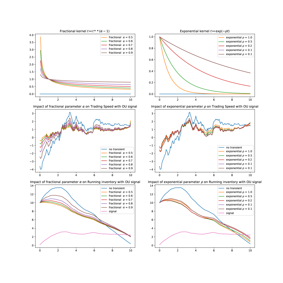
Figure 5: Impact of parameters of the kernels on the optimal trading speed and inventory with Ornstein-Uhlenbeck signal for the parameters $h_{0}\equiv 0,q_{0}=10,T=10,\lambda=0.5,\varrho=2,\phi=0$; for the OU signal: $I_{0}=2,\gamma=0.3,\sigma=0.5$. First column: Fractional kernel; Second column: Exponential kernel.

6 Derivation of the solution

6.1 The covariance operator

We define $\bm{\Sigma}_{t}$ the covariance operator induced by $K$ (recall (3.7)), as the integral operator associated with the following kernel:

$${\Sigma}_{t}(s,u)=\frac{1}{4\lambda}\int_{t}^{s\wedge u}K(s,z)K^{\top}(u,z)dz,\quad t\leq s,u\leq T,$$ (6.1)

where we recall that $\lambda$ is as in (2.4). Let ${\rm id}$ denotes the identity operator, i.e. $({\rm id}f)=f$ for all $f\in L^{2}\left([0,T],{\mathbb{R}}^{2}\right)$.

We define $\bm{\hat{K}}$ as the integral operator induced by the kernel $K$ as follows,

$$\hat{K}(t,s)=-K(t,s)\otimes e_{1},\quad\mbox{with }e_{1}=(1,0)^{\top},$$ (6.2)

where $\otimes$ represents the outer product. Specifically, we have

$$\hat{K}(t,s)=\begin{pmatrix}-\tilde{G}(t,s)&0\\ \mathds{1}_{\{s\leq t\}}&0\\ \end{pmatrix}.$$ (6.3)

We define the adjusted covariance integral operator $\bm{\tilde{\Sigma}}_{t}$ as follows

$$\bm{\tilde{\Sigma}}_{t}=\left({\rm id}-\frac{1}{2\lambda}\bm{\hat{K}}\right)^{-1}\bm{\Sigma}_{t}\left({\rm id}-\frac{1}{2\lambda}\bm{\hat{K}}^{*}\right)^{-1}.$$ (6.4)

Note that Lemma A.5 in [1] ensures that $\left({\rm id}-\frac{1}{2\lambda}\bm{\hat{K}}\right)$ and $\left({\rm id}-\frac{1}{2\lambda}\bm{\hat{K}}^{*}\right)$ are invertible.

6.2 The Riccati operator

We let

$$A=\left(\begin{matrix}\frac{1}{2\lambda}&0\\ 0&-2\phi\end{matrix}\right).$$ (6.5)

Recall that $\bm{\tilde{\Sigma}}_{t}$ was defined in (6.4). We define

$$\bm{\Psi}_{t}=\left({\rm id}-\frac{1}{2\lambda}\bm{\hat{K}}^{*}\right)^{-1}A\left({\rm id}-2\bm{\tilde{\Sigma}}_{t}A\right)^{-1}\left({\rm id}-\frac{1}{2\lambda}\bm{\hat{K}}\right)^{-1},\quad t\leq T.$$ (6.6)

First we identify $\bm{\Psi}_{t}$ with $\bm{\Gamma}^{-1}_{t}$ from (4.4), on a certain class of test functions. Recall that the notation $\mathds{1}_{t}$ was introduced in (4.6).

Lemma 6.1.

The operator $\bm{\Psi}_{t}$ satisfies for any $f\in L^{2}([0,T],{\mathbb{R}}^{2})$,

$$\mathds{1}_{t}(s)\big{(}\bm{\Psi}_{t}f\mathds{1}_{t}\big{)}(s)=\mathds{1}_{t}(s)\big{(}\bm{\Gamma}^{-1}_{t}f\mathds{1}_{t}\big{)}(s),\quad\textrm{for all }s,t\in[0,T].$$ (6.7)

The proof of Lemma 6.1 is given in Section 11.

We will show that $\bm{\Psi}_{t}$ is a solution to a Riccati operator equation involving the covariance operator $\bm{\Sigma}_{t}$ induced by the kernel (6.1). For this we specify our notion of differentiability: for any operator $\bm{G}$ from $L^{2}\left([0,T],{{\mathbb{R}}^{2}}\right)$ to itself we define the operator norm,

$$\|\bm{G}\|_{\rm{op}}=\sup_{f\in L^{2}([0,T],{\mathbb{R}}^{2})}\frac{\|\mathbb{G}f\|_{L^{2}}}{\|f\|_{L^{2}}}.$$ (6.8)

The operator $t\mapsto\bm{\Psi}_{t}$ is said to be strongly differentiable at time $t\geq 0$, if there exists a bounded linear operator $\dot{\bm{\Psi}}_{t}$ from $L^{2}\left([0,T],{{\mathbb{R}}}\right)$ into itself such that

$$\lim_{h\to 0}\frac{1}{h}\|\bm{\Psi}_{t+h}-\bm{\Psi}_{t}-h\dot{\bm{\Psi}}_{t}\|_{\rm{op}}=0.$$ (6.9)

The following lemma gives some fundamental properties of $\bm{\Psi}_{t}$ that will be useful for the proof of Theorem 4.4. Recall that $A$ was defined in (6.5) and $\bm{\hat{K}}$ was defined in (6.2).

Lemma 6.2.

For any $0\leq t\leq T$, $\bm{\Psi}_{t}$ given by (6.6) is a bounded linear operator from $L^{2}\left([0,T],{\mathbb{R}}\right)$ into itself. Moreover we have,

• $\bar{\bm{\Psi}}_{t}=(-A\cdot{\rm id}+\bm{\Psi}_{t})$ is an integral operator induced by a symmetric kernel $\bar{\psi}_{t}(s,u)$ that satisfies

  $$\sup_{t\leq T}\int_{[0,T]^{2}}|\bar{\psi}_{t}(s,u)|^{2}dsdu<\infty.$$

• For any $f\in L^{2}\left([0,T],{\mathbb{R}}^{2}\right)$,

  $$(\bm{\Psi}_{t}f\mathds{1}_{t})(t)=\left(A\cdot{\rm id}+\frac{1}{2\lambda}\bm{\hat{K}}^{*}\bm{\Psi}_{t}\right)(f\mathds{1}_{t})(t),$$

  where $\mathds{1}_{t}(s)=\mathds{1}_{\{t\leq s\}}$.

• $t\mapsto\bm{\Psi}_{t}$ is strongly differentiable and satisfies the operator Riccati equation

  $$\dot{\bm{\Psi}}_{t} =2\bm{\Psi}_{t}\dot{\bm{{\Sigma}}}_{t}\bm{\Psi}_{t},\qquad t\in[0,T],$$

  $${\bm{\Psi}_{T}} =\left({\rm id}-\frac{1}{2\lambda}\bm{\hat{K}}^{*}\right)^{-1}A\left({\rm id}-\frac{1}{2\lambda}\bm{\hat{K}}\right)^{-1},$$

  where $\dot{\bm{{\Sigma}}}_{t}$ is the strong derivative of $t\mapsto\mathbb{\Sigma}_{t}$ induced by the kernel

  $$\dot{\Sigma}_{t}(s,u)=-\frac{1}{4\lambda}K(s,t)K(u,t)^{\top},\quad a.e.$$ (6.10)

Proof.

The proof of (i) follows from (6.7) and Lemma 7.3. The proof of (ii) in given in Section 10. The proof of (iii) follows the same lines as the proof of Lemma 5.6 in [3] hence it is omitted. ∎

6.3 $L^{2}$–valued BSDE

In the following proposition we show that $\Theta=\{\Theta_{\cdot}(s):s\in[0,T]\}$ in (4.7) is a solution to an $L^{2}$-valued linear BSDE that involves the operator $\bm{\Psi}_{t}$ and the kernel $\bar{\psi}_{t}$ appearing in Lemma 6.2.

Proposition 6.3.

For each $s\leq T$, the process $\Theta$ solves the following $L^{2}$–valued BSDE,

$$d\Theta_{t}(s) =\dot{\Theta}_{t}(s)dt+dN_{t}(s),\quad 0\leq t<s,$$ (6.11)

$$\textrm{with }\dot{\Theta}_{t}(s) =2\big{(}\bm{{\Psi}}_{t}\dot{\bm{\Sigma}}_{t}\Theta_{t}\big{)}(s)-\bar{\psi}_{t}(s,t){\mathbb{E}}_{t}[P_{t}-P_{T}]e_{1},$$

with the following boundary condition

$$\Theta_{s}(s)=-\frac{1}{2\lambda}\left(P_{s}-{\mathbb{E}}_{s}[P_{T}]+\langle\Theta_{s},K_{s}\rangle_{L^{2}}\right)e_{1},$$ (6.12)

where for each $0\leq s\leq T$, $\{N_{t}(s)\}_{t\geq 0}$ is a suitable square-integrable martingale.

The proof of Proposition is postponed to Section 9.

6.4 A verification result

We will use the following lemma that derives the general dynamics for some functionals in $L^{2}$.

Lemma 6.4.

Let $f(t,s)$ and $h(t,s)$ be two $L^{2}([0,T]^{2},\mathds{R}^{2})$ functions that are continuous in $(t,s)\in[0,T]^{2}$, with partial derivatives with respect to $t$, $\dot{f}(t,s):=\partial_{t}f(t,s)$, $\dot{h}(t,s):=\partial_{t}h(t,s)$ that are in $L^{2}([0,T]^{2},\mathds{R}^{2})$. Define

$$F_{t}(s)=\mathds{1}_{\{t\leq s\}}f(t,s),\quad\textrm{and }H_{t}(s)=\mathds{1}_{\{t\leq s\}}h(t,s).$$ (6.13)

Let $\bm{\Xi}_{t}:=A{\rm id}+\bar{\bm{\Xi}}_{t}$ where $\bar{\bm{\Xi}}_{t}$ a bounded, strongly differentiable and self adjoint integral operator in $L^{2}$, and $A$ is a $2\times 2$ symmetric matrix. Then, the derivative of $t\mapsto\langle F_{t},\bm{\Xi}_{t}H_{t}\rangle_{L^{2}}$ is given by

$$\frac{d}{dt}\langle F_{t},\bm{\Xi}_{t}H_{t}\rangle_{L^{2}} =-f^{\top}(t,t)Ah(t,t)-f^{\top}(t,t)\bar{\bm{\Xi}}_{t}H_{t}(t)+\langle\mathds{1}_{t}\dot{f}(t,\cdot),{\bm{\Xi}}_{t}H_{t}\rangle_{L^{2}}$$

$$\quad+\langle F_{t},\dot{{\bm{\Xi}}}_{t}H_{t}\rangle_{L^{2}}-h(t,t)^{\top}\bar{\bm{\Xi}}_{t}F_{t}(t)+\langle F_{t},{\bm{\Xi}}_{t}\mathds{1}_{t}\dot{h}_{t}\rangle_{L^{2}}.$$

Proof.

We first use the following decomposition

$$\langle F_{t},\bm{\Xi}_{t}H_{t}\rangle_{L^{2}}=\langle F_{t},\bar{\bm{\Xi}}_{t}H_{t}\rangle_{L^{2}}+\langle F_{t},(A{\rm id})H_{t}\rangle_{L^{2}}.$$ (6.14)

Recall that $(A{\rm id})H_{t}=AH_{t}$. A direct application of (6.13), (2.13) and a generalized version of Leibnitz’s rule (see e.g. Lemma 2.14 in [29]) gives

$$\frac{d}{dt}\langle F_{t},(A{\rm id})H_{t}\rangle_{L^{2}} =\frac{d}{dt}\int_{t}^{T}f^{\top}(t,s)Ah(t,s)ds$$ (6.15)

$$=-f^{\top}(t,t)Ah(t,t)+\int_{t}^{T}{\dot{f}}^{\top}(t,s)Ah(t,s)ds$$

$$\quad+\int_{t}^{T}f^{\top}(t,s)A\dot{h}(t,s)ds$$

$$=-f^{\top}(t,t)Ah(t,t)+\int_{0}^{T}\mathds{1}_{\{s\geq t\}}{\dot{f}}^{\top}(t,s)AH_{t}(s)ds$$

$$\quad+\int_{0}^{T}F_{t}^{\top}(s)A\mathds{1}_{\{s\geq t\}}\dot{h}(t,s)ds$$

$$=-f^{\top}(t,t)Ah(t,t)+\langle{\mathds{1}_{t}\dot{f}}(t,\cdot),A{\rm id}H_{t}\rangle_{L^{2}}$$

$$\quad+\langle F_{t},A{\rm id}\mathds{1}_{t}\dot{h}(t,\cdot)\rangle_{L^{2}},$$

where we used $({\rm id}H_{t})(s)=H_{t}(s)$ in the last line.

Using similar arguments, we get

$$\frac{d}{dt}\langle F_{t},\bar{\bm{\Xi}}_{t}H_{t}\rangle_{L^{2}} =\frac{d}{dt}\int_{t}^{T}f^{\top}(t,s)\bar{\bm{\Xi}}_{t}H_{t}(s)ds$$ (6.16)

$$=-f^{\top}(t,t)\bar{\bm{\Xi}}_{t}H_{t}(t)+\int_{t}^{T}\dot{f}^{\top}(t,s)\bar{\bm{\Xi}}_{t}H_{t}(s)ds$$

$$\quad+\int_{t}^{T}f^{\top}(t,s)\frac{d}{dt}\left(\bar{\bm{\Xi}}_{t}H_{t}(s)\right)ds$$

$$=-f^{\top}(t,t)\bar{\bm{\Xi}}_{t}H_{t}(t)+\langle\mathds{1}_{t}\dot{f}(t,\cdot),\bar{\bm{\Xi}}_{t}H_{t}\rangle_{L^{2}}$$

$$\quad+\int_{t}^{T}f^{\top}(t,s)\frac{d}{dt}\left(\bar{\bm{\Xi}}_{t}H_{t}(s)\right)ds.$$

Note that

$$\frac{d}{dt}\left(\bar{\bm{\Xi}}_{t}H_{t}(s)\right) =\frac{d}{dt}\int_{t}^{T}\bar{\Xi}_{t}(s,r)h(t,r)dr$$ (6.17)

$$=-\bar{\Xi}_{t}(s,t)h(t,t)+\int_{t}^{T}\left(\frac{d}{dt}\bar{\Xi}_{t}(s,r)\right)h(t,r)dr$$

$$\quad+\int_{t}^{T}\bar{\Xi}_{t}(s,r)\dot{h}(t,r)dr$$

$$=-\bar{\Xi}_{t}(t,r)h(t,t)+\dot{\bar{\bm{\Xi}}}_{t}H_{t}(s)+\bar{\bm{\Xi}}_{t}\mathds{1}_{t}\dot{h}(t,\cdot)(s),$$

where we used the fact that the kernel of the operator $\dot{\bar{\bm{\Xi}}}_{t}$ is $\dot{\bar{{\Xi}}}_{t}$ in the last line.

From (6.17) and since $\bar{\bm{\Xi}}_{t}$ is self adjoint, we get that

$$\int_{t}^{T}f^{\top}(t,s)\frac{d}{dt}\left(\bar{\bm{\Xi}}_{t}H_{t}(s)\right)ds$$ (6.18)

$$=-\int_{t}^{T}f^{\top}(t,s)\bar{\Xi}_{t}(s,t)h(t,t)ds+\int_{t}^{T}f^{\top}(t,s)\dot{\bar{\bm{\Xi}}}_{t}H_{t}(s)ds$$

$$\quad+\int_{t}^{T}f^{\top}(t,s)\bar{\bm{\Xi}}_{t}\mathds{1}_{t}\dot{h}(t,\cdot)(s)ds$$

$$=-h(t,t)^{\top}\bar{\bm{\Xi}}_{t}F_{t}(t)+\langle F_{t},\bar{\bm{\Xi}}_{t}\mathds{1}_{t}\dot{h}_{t}\rangle_{L^{2}}+\langle F_{t},\dot{\bar{\bm{\Xi}}}_{t}H_{t}\rangle_{L^{2}}.$$

From (6.16) and (6.18) it follows that

$$\frac{d}{dt}\langle F_{t},\bar{\bm{\Xi}}_{t}H_{t}\rangle_{L^{2}} =-f^{\top}(t,t)\bar{\bm{\Xi}}_{t}H_{t}(t)+\langle\mathds{1}_{t}\dot{f}(t,\cdot),\bar{\bm{\Xi}}_{t}H_{t}\rangle_{L^{2}}$$ (6.19)

$$\quad-h(t,t)^{\top}\bar{\bm{\Xi}}_{t}F_{t}(t)+\langle F_{t},\bar{\bm{\Xi}}_{t}\mathds{1}_{t}\dot{h}_{t}\rangle_{L^{2}}+\langle F_{t},\dot{\bar{\bm{\Xi}}}_{t}H_{t}\rangle_{L^{2}}.$$

Applying (6.15) and (6.19) to (6.14) we finally get

$$\frac{d}{dt}\langle F_{t},{\bm{\Xi}}_{t}H_{t}\rangle_{L^{2}} =-f^{\top}(t,t)\bar{\bm{\Xi}}_{t}H_{t}(t)+\langle\mathds{1}_{t}\dot{f}(t,\cdot),\bar{\bm{\Xi}}_{t}H_{t}\rangle_{L^{2}}$$

$$\quad-h(t,t)^{\top}\bar{\bm{\Xi}}_{t}F_{t}(t)+\langle F_{t},\bar{\bm{\Xi}}_{t}\mathds{1}_{t}\dot{h}_{t}\rangle_{L^{2}}+\langle F_{t},\dot{\bar{\bm{\Xi}}}_{t}H_{t}\rangle$$

$$\quad-f^{\top}(t,t)Ah(t,t)+\langle{\bm{1}_{t}\dot{f}}(t,\cdot),A{\rm id}H_{t}\rangle_{L^{2}}$$

$$\quad+\langle F_{t},A{\rm id}\mathds{1}_{t}\dot{h}(t,\cdot)\rangle_{L^{2}}$$

$$=-f^{\top}(t,t)Ah(t,t)-f^{\top}(t,t)\bar{\bm{\Xi}}_{t}H_{t}(t)+\langle\mathds{1}_{t}\dot{f}(t,\cdot),{\bm{\Xi}}_{t}H_{t}\rangle_{L^{2}}$$

$$\quad+\langle F_{t},\dot{{\bm{\Xi}}}_{t}H_{t}\rangle_{L^{2}}-h(t,t)^{\top}\bar{\bm{\Xi}}_{t}F_{t}(t)+\langle F_{t},{\bm{\Xi}}_{t}\mathds{1}_{t}\dot{h}_{t}\rangle_{L^{2}},$$

were we used $\bm{\Xi}_{t}:=A{\rm id}+\bar{\bm{\Xi}}_{t}$ and $\dot{\bm{\Xi}}_{t}=\dot{\bar{\bm{\Xi}}}_{t}$ in the last line. This completes the proof.

∎

We will use Lemma 6.4 in order to differentiate the first term on the right hand side of (4.12). Recall that for $K$ as in (3.7) we write $K_{t}(s)=K(s,t)$.

Lemma 6.5.

Let $g^{u}$ as in (3.8) and $\bm{\Psi}$ as in (6.6) then we have

$$\frac{d}{dt}\langle g^{u}_{t},\bm{\Psi}_{t}g_{t}^{u}\rangle_{L^{2}} =-(g^{u}_{t}(t))^{\top}Ag^{u}_{t}(t)+\frac{1}{\lambda}g^{u}_{t}(t)^{\top}\left(\bm{\hat{K}}^{*}\bm{\Psi}_{t}\right)(g^{u}_{t}\mathds{1}_{t})(t)$$

$$\quad+2\langle{\bm{\Psi}}_{t}K_{t},g^{u}_{t}\rangle_{L^{2}}u_{t}+2\langle g^{u}_{t},\bm{\Psi}_{t}\dot{\bm{{\Sigma}}}_{t}\bm{\Psi}_{t}g^{u}_{t}\rangle_{L^{2}}.$$

Proof.

Define

$$\tilde{g}^{u}_{t}(s):=g_{0}(s)+\int_{0}^{t}K(s,r)u_{r}dr,\quad 0\leq s,t\leq T,$$ (6.20)

where $g_{0}$ was defined in (3.7). From (2.13) and an application of Cauchy-Schwarz inequality it follows that $\tilde{g}^{u}_{t}(s)$ is continuous in $(t,s)\in[0,T]^{2}$, as required by the assumptions of Lemma 6.4.

From (6.20) we get that

$$\frac{d}{dt}\tilde{g}^{u}_{t}(s)=K(s,t)u_{t}=K_{t}(s)u_{t},\quad\textrm{for all }0<t,s\leq T.$$ (6.21)

Moreover, from (3.8) we have

$$g^{u}_{t}(s)=\mathds{1}_{\{t\leq s\}}\tilde{g}^{u}_{t}(s),\quad\textrm{for all }0<t,s\leq T.$$ (6.22)

From Lemma 6.2(i) it follows that,

$$\bm{\Psi}_{t}=A\cdot{\rm id}+\bar{\bm{\Psi}}_{t},$$ (6.23)

where $\bar{\bm{\Psi}}_{t}$ is a self adjoint integral operator.

From (6.21)-(6.23) and by a direct application of Lemma 6.4 we get

$$\frac{d}{dt}\langle g_{t}^{u},\bm{\Psi}_{t}g_{t}^{u}\rangle_{L^{2}} =-(\tilde{g}^{u}_{t}(t))^{\top}A\tilde{g}^{u}_{t}(t)-(\tilde{g}^{u}_{t}(t))^{\top}\bar{\bm{\Psi}}_{t}{g}^{u}_{t}(t)+\langle\mathds{1}_{t}\dot{\tilde{g}}^{u}_{t},{\bm{\Psi}}_{t}g^{u}_{t}\rangle_{L^{2}}$$ (6.24)

$$\quad+\langle g^{u}_{t},\dot{{\bm{\Psi}}}_{t}g^{u}_{t}\rangle_{L^{2}}-\tilde{g}_{t}^{u}(t)^{\top}\bar{\bm{\Psi}}_{t}g^{u}_{t}(t)+\langle g^{u}_{t},{\bm{\Psi}}_{t}\mathds{1}_{t}\dot{\tilde{g}}^{u}_{t}\rangle_{L^{2}}$$

$$=-(\tilde{g}^{u}_{t}(t))^{\top}A\tilde{g}^{u}_{t}(t)-(\tilde{g}^{u}_{t}(t))^{\top}(-A\cdot{\rm id}+\bm{\Psi}_{t}){g}^{u}_{t}(t)+\langle\mathds{1}_{t}K_{t},{\bm{\Psi}}_{t}g^{u}_{t}\rangle_{L^{2}}u_{t}$$

$$\quad+\langle g^{u}_{t},\dot{{\bm{\Psi}}}_{t}g^{u}_{t}\rangle_{L^{2}}-\tilde{g}_{t}^{u}(t)^{\top}(-A\cdot{\rm id}+\bm{\Psi}_{t})g^{u}_{t}(t)+\langle g^{u}_{t},{\bm{\Psi}}_{t}\mathds{1}_{t}K_{t}\rangle_{L^{2}}u_{t}.$$

Since $A$ is a symmetric matrix and $\bar{\bm{\Psi}}_{t}$ is self-adjoint, it follows from (6.23) that ${\bm{\Psi}}_{t}$ is self-adjoint. Together with (6.22) we get that,

$$\langle\mathds{1}_{t}K_{t},{\bm{\Psi}}_{t}g^{u}_{t}\rangle_{L^{2}} =\langle g^{u}_{t},{\bm{\Psi}}_{t}\mathds{1}_{t}K_{t}\rangle_{L^{2}}$$ (6.25)

$$=\langle{\bm{\Psi}}_{t}K_{t},g^{u}_{t}\rangle_{L^{2}}.$$

From (6.22) we also have $g^{u}_{t}(t)=\tilde{g}^{u}_{t}(t)$. Using this and (6.25), we can gather similar terms in (6.24) and get,

$$\frac{d}{dt}\langle g_{t}^{u},\bm{\Psi}_{t}g_{t}^{u}\rangle_{L^{2}} =(g^{u}_{t}(t))^{\top}Ag^{u}_{t}(t)-2g^{u}_{t}(t)^{\top}({\bm{\Psi}}_{t}g^{u}_{t})(t)$$

$$\quad+2\langle{\bm{\Psi}}_{t}K_{t},g^{u}_{t}\rangle_{L^{2}}u_{t}+\langle g^{u}_{t},\dot{\bm{\Psi}}_{t}g^{u}_{t}\rangle_{L^{2}}.$$

Together with Lemma 6.2(iii) and (iv) it follows that

$$\frac{d}{dt}\langle g_{t}^{u},\bm{\Psi}_{t}g_{t}^{u}\rangle_{L^{2}} =-(g^{u}_{t}(t))^{\top}Ag^{u}_{t}(t)+\frac{1}{\lambda}g^{u}_{t}(t)^{\top}\left(\bm{\hat{K}}^{*}\bm{\Psi}_{t}\right)(g^{u}_{t}\mathds{1}_{t})(t)$$

$$\quad+2\langle{\bm{\Psi}}_{t}K_{t},g^{u}_{t}\rangle_{L^{2}}u_{t}+2\langle g^{u}_{t},\bm{\Psi}_{t}\dot{\bm{{\Sigma}}}_{t}\bm{\Psi}_{t}g^{u}_{t}\rangle_{L^{2}},$$

which completes the proof. ∎

We now use Lemma 6.4 to differentiate the second term on the right hand side of (4.12).

Lemma 6.6.

Let $g^{u}$ as in (3.8) and $\Theta_{t}$ as in (6.11) . Then we have

$$d\langle{\Theta}_{t},g_{t}^{u}\rangle_{L^{2}} =\left(2\langle\bm{\Psi}_{t}\dot{\bm{\Sigma}}_{t}\Theta_{t},g_{t}^{u}\rangle_{L^{2}}-\frac{1}{2\lambda}(P_{t}-M_{t})\langle\bm{\Psi}_{t}K_{t},g_{t}^{u}\rangle_{L^{2}}\right)dt$$

$$\quad+\left(\langle{\Theta}_{t},K_{t}\rangle_{L^{2}}u_{t}+\frac{1}{2\lambda}\left(P_{t}-M_{t}+\langle\Theta_{t},K_{t}\rangle_{L^{2}}\right)Y^{u}_{t}\right)dt+\langle dN_{t},g_{t}^{u}\rangle_{L^{2}}.$$

Proof.

First note that Lemma 6.2(i) and (ii) can be applied to $g_{t}^{u}$ instead of $f$, as time dependence will not change the result. Together with (3.7), (6.3) and (3.8) we get,

$$\langle\bar{\psi}_{t}(\cdot,t)e_{1},g_{t}^{u}\rangle_{L^{2}} =e_{1}^{\top}\int_{t}^{T}\bar{\psi}_{t}(t,s)g_{t}^{u}(s)ds$$ (6.26)

$$=e_{1}^{\top}(\bm{\Psi}_{t}-A{\rm id})(g^{u}_{t}\mathds{1}_{t})(t)$$

$$=\frac{1}{2\lambda}e_{1}^{\top}(\hat{\bm{K}}^{*}\bm{\Psi}_{t})(g^{u}_{t}\mathds{1}_{t})(t)$$

$$=-\frac{1}{2\lambda}e_{1}^{\top}e_{1}\langle\bm{\Psi}_{t}K_{t},g^{u}_{t}\mathds{1}_{t}\rangle_{L^{2}}$$

$$=-\frac{1}{2\lambda}\langle\bm{\Psi}_{t}K_{t},g^{u}_{t}\mathds{1}_{t}\rangle_{L^{2}}.$$

Using Leibnitz rule and (6.22), we get

$$d\langle{\Theta}_{t},g_{t}^{u}\rangle_{L^{2}} =d\int_{t}^{T}\Theta^{\top}_{t}(s)\tilde{g}_{t}^{u}(s)ds$$ (6.27)

$$=-\Theta_{t}(t)^{\top}g_{t}(t)dt+\int_{t}^{T}d\big{(}\Theta_{t}^{\top}(s){\tilde{g}}_{t}^{u}(s)\big{)}ds.$$

From Itô product rule, (6.11) and (6.21) we have

$$d\big{(}\Theta^{\top}_{t}(s)\tilde{g}_{t}^{u}(s)\big{)} =\tilde{g}_{t}^{u}(s)d\Theta^{\top}_{t}(s)+\Theta_{t}^{\top}(s)\dot{\tilde{g}}_{t}^{u}(s)$$ (6.28)

$$=(\dot{\Theta}^{\top}_{t}(s)dt+dN^{\top}_{t})\tilde{g}_{t}^{u}(s)+\Theta^{\top}_{t}(s)\dot{\tilde{g}}_{t}^{u}(s)dt.$$

From (6.21), (6.27) and (6.28) we get,

$$d\langle{\Theta}_{t},g_{t}^{u}\rangle_{L^{2}} =\left(\langle\dot{\Theta}_{t},g_{t}^{u}\rangle_{L^{2}}+\langle{\Theta}_{t},K_{t}\rangle_{L^{2}}u_{t}-\Theta_{t}(t)^{\top}g_{t}(t)\right)dt+\langle dN_{t},g_{t}^{u}\rangle_{L^{2}}.$$

Together with (3.9), (6.11), (6.12) and (6.26) we get

$$d\langle{\Theta}_{t},g_{t}^{u}\rangle_{L^{2}} =\left(2\langle\bm{\Psi}_{t}\dot{\bm{\Sigma}}_{t}\Theta_{t},g_{t}^{u}\rangle_{L^{2}}-\frac{1}{2\lambda}(P_{t}-M_{t})\langle\bm{\Psi}_{t}K_{t},g_{t}^{u}\rangle_{L^{2}}\right)dt$$

$$\quad+\left(\langle{\Theta}_{t},K_{t}\rangle_{L^{2}}u_{t}+\frac{1}{2\lambda}\left(P_{t}-M_{t}+\langle\Theta_{t},K_{t}\rangle_{L^{2}}\right)Y^{u}_{t}\right)dt+\langle dN_{t},g_{t}^{u}\rangle_{L^{2}}.$$

∎

We now we are ready to prove Theorem 4.4.

Proof of Theorem 4.4.

Recall that the proposed value process $V_{t}$ was defined in (4.12) and the performance functional $J$ was defined in (3.3). For any admissible $u$ as in (2.3) we set

$$J_{t}(u)={\mathbb{E}}\left[\int_{t}^{T}\left((P_{s}-Y^{u}_{s})u_{s}-\lambda u_{s}^{2}-\phi(Q^{u}_{s})^{2}\right)ds+P_{T}Q^{u}_{T}-\varrho q^{2}{\ \Big{|}\ }\mathcal{F}_{t}\right],$$ (6.29)

and we define the process

$$M^{u}_{t}=\int_{0}^{t}\left((P_{s}-Y^{u}_{s})u_{s}-\lambda u_{s}^{2}-\phi(Q^{u}_{s})^{2}\right)ds+V_{t}^{u}+\lambda\int_{0}^{t}(u_{s}-{\mathcal{T}_{s}(u)})^{2}ds,$$ (6.30)

where

$${\mathcal{T}_{t}(u)}=\frac{1}{2\lambda}\big{(}{\mathbb{E}}[(P_{t}-P_{T})\mid\mathcal{F}_{t}]-Y^{u}_{t}+\langle\Theta_{t},K_{t}\rangle_{L^{2}}+\langle\bm{\Psi}_{t}K_{t},g_{t}^{u}\rangle_{L^{2}}\big{)}.$$ (6.31)

The following proposition, which will be proved at the end of this section is an important ingredient for the proof.

Proposition 6.7.

For any $u$ $\in$ $\mathcal{A}$, $M^{u}$ is a martingale with respect to $(\mathcal{F}_{t})_{0\leq t\leq T}$.

Proposition 6.7 implies that

$${\mathbb{E}}[M^{u}_{T}|\mathcal{F}_{t}]=M^{u}_{t},\quad\textrm{for all }0\leq t\leq T.$$ (6.32)

From (3.8) it follows that $g_{T}(s)=0$ on $[0,T)$. From (4.10) we have $\chi_{T}=-2\varrho q^{2}$. Using both terminal conditions on (4.12) give,

$$V_{T}^{u} =\frac{1}{2}\langle g_{T}^{u},\bm{\Psi}_{T}g_{T}^{u}\rangle_{L^{2}}+\langle\Theta_{T},g_{T}^{u}\rangle_{L^{2}}+\mathbb{E}[P_{T}\mid\mathcal{F}_{T}]Q_{T}^{u}+\frac{1}{2}\chi_{T}$$ (6.33)

$$=P_{T}Q_{T}^{u}-\varrho q^{2}.$$

By using (6.32) and (6.33) on (6.29) and (6.30) it follows that

$$V_{t}^{u}-J_{t}(u) =\lambda{\mathbb{E}}\left[\int_{t}^{T}(u_{s}-{\mathcal{T}_{s}(u)})^{2}ds{\ \Big{|}\ }\mathcal{F}_{t}\right].$$ (6.34)

Since $\lambda>0$, the right hand side of (6.34) is always nonnegative and it vanishes for $u=u^{*}$, where $u^{*}(\cdot)=\mathcal{T}_{\cdot}(u^{*})$ is given by (4.14).

Fix now $t\leq T$ and recall that $\mathcal{A}_{t}(u^{*})$ was defined in (4.2). We observe that $V_{t}^{u^{*}}$ $=$ $V_{t}^{u^{\prime}}$ for all $u^{\prime}$ $\in$ $\mathcal{A}_{t}(u^{*})$. We then deduce from (6.34) that

$$V_{t}^{u^{*}} =J_{t}(u^{*})\;=\;\operatorname*{ess~{}sup}_{u^{\prime}\in\mathcal{A}_{t}(u^{*})}J_{t}(u^{\prime}),$$

which is equivalent to (4.13). This proves that $u^{*}$ is an optimal control. ∎

Proof of Proposition 6.7.

Recall that $M_{t}={\mathbb{E}}[P_{T}|\mathcal{F}_{t}]$ and define

$$\beta_{t}=P_{t}-M_{t}+\langle\Theta_{t},K_{t}\rangle_{L^{2}}.$$ (6.35)

Then from (4.8), (6.30), (6.31) and (6.35) we have

$$dM^{u}_{t} =\left((P_{t}-Y^{u}_{t})u_{t}-\lambda u_{t}^{2}-\phi(Q^{u}_{t})^{2}+\lambda(u_{t}-{\mathcal{T}_{t}(u)})^{2}\right)dt+dV_{t}^{u}$$ (6.36)

$$=\big{(}(P_{t}-Y^{u}_{t})u_{t}-\phi(Q^{u}_{t})^{2}-2\lambda{\mathcal{T}_{t}(u)}u_{t}+\lambda{\mathcal{T}_{t}(u)}^{2}\big{)}dt+dV_{t}^{u}$$

$$=-\phi(Q^{u}_{t})^{2}dt-\left(-M_{t}+\langle\Theta_{t},K_{t}\rangle_{L^{2}}+\langle\bm{\Psi}_{t}K_{t},g_{t}^{u}\rangle_{L^{2}}\right)u_{t}\big{)}dt$$

$$\quad+\frac{1}{4\lambda}\left(\beta_{t}-Y^{u}_{t}+\langle\bm{\Psi}_{t}K_{t},g_{t}^{u}\rangle_{L^{2}}\right)^{2}dt+dV_{t}^{u}$$

$$=\left(\frac{1}{2}g^{u}_{t}(t)^{\top}Ag^{u}_{t}(t)-\left(-M_{t}+\langle\Theta_{t},K_{t}\rangle_{L^{2}}+\langle\bm{\Psi}_{t}K_{t},g_{t}^{u}\rangle_{L^{2}}\right)u_{t}\right)dt$$

$$\quad+\frac{1}{4\lambda}\left(\beta_{t}^{2}+2\beta_{t}\langle\bm{\Psi}_{t}K_{t},g_{t}^{u}\rangle_{L^{2}}-2\beta_{t}Y_{t}^{u}-2Y_{t}^{u}\langle\bm{\Psi}_{t}K_{t},g_{t}^{u}\rangle_{L^{2}}+\langle\bm{\Psi}_{t}K_{t},g_{t}^{u}\rangle_{L^{2}}^{2}\right)dt$$

$$\quad+dV_{t}^{u},$$

where we have used the identity

$$g^{u}_{t}(t)^{\top}Ag^{u}_{t}(t)=\frac{1}{2\lambda}(Y^{u}_{t})^{2}-2\phi(Q^{u}_{t})^{2},$$

which follows from (3.9) and (6.5), in the last equality.

An application of (4.11) and Lemmas 6.5 and 6.6 to (4.12) yields:

$$dV^{u}_{t} ={\frac{1}{2}}\bigg{(}\left(-g^{u}_{t}(t)^{\top}Ag^{u}_{t}(t)+\frac{{1}}{\lambda}g^{u}_{t}(t)^{\top}\left(\bm{\hat{K}}^{*}\bm{\Psi}_{t}\right)(g^{u}_{t}\mathds{1}_{t})(t)\right)dt$$ (6.37)

$$\quad+\left(2\langle{\bm{\Psi}}_{t}K_{t},g^{u}_{t}\rangle_{L^{2}}u_{t}+2\langle g^{u}_{t},\bm{\Psi}_{t}\dot{\bm{{\Sigma}}}_{t}\bm{\Psi}_{t}g^{u}_{t}\rangle_{L^{2}}\right)dt$$

$$\quad+\left(4\langle\bm{\Psi}_{t}\dot{\bm{\Sigma}}_{t}\Theta_{t},g_{t}^{u}\rangle_{L^{2}}-\frac{1}{\lambda}(P_{t}-M_{t})\langle\bm{\Psi}_{t}K_{t},g_{t}^{u}\rangle_{L^{2}}\right)dt$$

$$\quad+\left(2\langle{\Theta}_{t},K_{t}\rangle_{L^{2}}u_{t}+\frac{{1}}{\lambda}\left(P_{t}-M_{t}+\langle\Theta_{t},K_{t}\rangle_{L^{2}}\right)Y^{u}_{t}\right)dt$$

$$\quad+\left(-2M_{t}u_{t}+\dot{\chi}_{t}\right)dt+\left(2Q^{u}_{t}+z_{t}^{\chi}\right)dM_{t}+2\langle dN_{t},g^{u}_{t}\rangle_{L^{2}}\bigg{)}.$$

Note that from (4.11) and (6.35) we have

$$\dot{\chi}_{t}=-\frac{1}{2\lambda}\beta_{t}^{2}.$$ (6.38)

Next we introduce the following lemma with some useful identities. Recall that the notation $\mathds{1}_{t}$ was introduced in (4.6).

Lemma 6.8.

The following identities hold:

• $$4\langle\bm{\Psi}_{t}\dot{\bm{\Sigma}}_{t}\Theta_{t},g_{t}^{u}\rangle_{L^{2}}=-\frac{1}{\lambda}\langle\bm{\Psi}_{t}K_{t},g_{t}^{u}\rangle_{L^{2}}\langle K_{t},\Theta_{t}\rangle_{L^{2}}.$$ (6.39)

• $$\left(\bm{\hat{K}}^{*}\bm{\Psi}_{t}\right)(g^{u}_{t}\mathds{1}_{t})(t)=-\langle\bm{\Psi}_{t}K_{t},g_{t}\rangle_{L^{2}}e_{1}.$$

• $$2\langle\bm{\Psi}_{t}\dot{\bm{\Sigma}}_{t}\bm{\Psi}_{t}g_{t}^{u},g_{t}^{u}\rangle_{L^{2}}=-\frac{1}{2\lambda}\langle\bm{\Psi}_{t}K_{t},g_{t}^{u}\rangle_{L^{2}}^{2}.$$ (6.40)

The proof of Lemma 6.8 is postponed to Section 8.

Using (6.38)–(6.40), we can rewrite (6.37) as

$$dV^{u}_{t} =\frac{1}{2}\bigg{(}\left(-g^{u}_{t}(t)^{\top}Ag^{u}_{t}(t)+\frac{1}{\lambda}g^{u}_{t}(t)^{\top}\langle\bm{\Psi}K_{t},g_{t}\rangle_{L^{2}}e_{1}\right)dt$$ (6.41)

$$\quad+\left(2\langle{\bm{\Psi}}_{t}K_{t},g^{u}_{t}\rangle_{L^{2}}u_{t}-\frac{1}{2\lambda}\langle\bm{\Psi}_{t}K_{t},g_{t}^{u}\rangle_{L^{2}}^{2}\right)dt$$

$$\quad-\frac{1}{\lambda}\left(\langle\bm{\Psi}_{t}K_{t},g_{t}^{u}\rangle_{L^{2}}\langle K_{t},\Theta_{t}\rangle_{L^{2}}+(P_{t}-M_{t})\langle\bm{\Psi}_{t}K_{t},g_{t}^{u}\rangle_{L^{2}}\right)dt$$

$$\quad+\left(2\langle{\Theta}_{t},K_{t}\rangle_{L^{2}}u_{t}+\frac{1}{\lambda}\left(P_{t}-M_{t}+\langle\Theta_{t},K_{t}\rangle_{L^{2}}\right)Y^{u}_{t}\right)dt$$

$$\quad-\left(2M_{t}u_{t}+\frac{1}{2\lambda}\beta_{t}^{2}\right)dt+\left(2Q^{u}_{t}+z_{t}^{\chi}\right)dM_{t}+2\langle dN_{t},g^{u}_{t}\rangle_{L^{2}}\bigg{)}.$$

Plugging in (6.41) to (6.36) and using (6.35) we get

$$dM^{u}_{t} =\left(\frac{1}{\lambda}g^{u}_{t}(t)^{\top}e_{1}\langle\bm{\Psi}K_{t},g_{t}\rangle_{L^{2}}-\frac{1}{\lambda}Y_{t}^{u}\langle\bm{\Psi}_{t}K_{t},g_{t}^{u}\rangle_{L^{2}}\right)dt$$

$$\quad+\left(2Q^{u}_{t}+z_{t}^{\chi}\right)dM_{t}+2\langle dN_{t},g^{u}_{t}\rangle_{L^{2}}.$$

From (3.9) we have $g^{u}_{t}(t)^{\top}e_{1}=Y_{t}^{u}$, so we get

$$dM_{t}^{u}=\left(2Q^{u}_{t}+z_{t}^{\chi}\right)dM_{t}+2\langle dN_{t},g^{u}_{t}\rangle_{L^{2}}.$$ (6.42)

This shows that $M^{u}$ is a local martingale. From (6.30), (7.4), (2.1), (2.3) and several applications of Cauchy-Schwarz inequality, it follows that $\sup_{t\in[0,T]}{\mathbb{E}}[(M_{t}^{u})^{2}]<\infty$, hence $M^{u}$ is a true martingale.

Note that the admissibility of $u^{*}$ follows from the explicit solution derived in Proposition 4.5 which is equivalent to (4.14) and from the bounds derived in Lemma 7.1. ∎

7 Proof of Proposition 4.5

Proof of Proposition 4.5.

Recalling (2.2) we note that $g^{u}$ defined in (3.8) can be re-written in the form

$$g_{t}^{u}(s)=\mathds{1}_{\{s\geq t\}}\left(\tilde{h}_{0}(s),q\right)^{\top}+\int_{0}^{t}\mathds{1}_{\{s\geq t\}}\left(\tilde{G}(s,r),-1\right)^{\top}u_{r}dr,$$

so that an application of Fubini’s theorem leads to

$$\langle\bm{\Gamma}_{t}^{-1}K_{t},g_{t}^{u}\rangle_{L^{2}}=\langle\bm{\Gamma}_{t}^{-1}K_{t},\mathds{1}_{t}\left(\tilde{h}_{0},q\right)^{\top}\rangle_{L^{2}}+\int_{0}^{t}\langle\bm{\Gamma}_{t}^{-1}K_{t},\mathds{1}_{t}\left(\tilde{G}(\cdot,r),-1\right)^{\top}\rangle_{L^{2}}u_{r}dr,$$

which, combined with (3.5), yields that we can rewrite (4.14) as (4.15). Note that (4.15) is a linear Volterra equation which admits a solution for any fixed $\omega\in\Omega$, whenever $a(\omega)\in L^{2}([0,T],\mathbb{R})$ and $B$ satisfies

$$\sup_{t\leq T}\int_{0}^{T}B(t,s)^{2}ds<\infty.$$

Indeed, the solution is given in terms of the resolvent $R^{B}$ of B, see (10.1) below, which exists by virtue of Corollary 9.3.16 in [26] and satisfies

$$\int_{0}^{T}\int_{0}^{T}|R^{B}(t,s)|dtds<\infty.$$

In this case, the solution $u^{*}$ is given by

$$u_{t}^{*}=a_{t}+\int_{0}^{t}R^{B}(t,s)a_{s}ds.$$

Note that $R^{B}$ is the kernel of the operator given by

$$\bm{R}^{B}=({\rm id}-\bm{B})^{-1}.$$

One would still need to check that $u^{*}\in\mathcal{A}$ defined as in (2.3). This follows from the following lemma, which will be proved in the end of this section.

Lemma 7.1.

Assume $\lambda>0$ and $\phi,\varrho\geq 0$. Then, the following hold:

• $\mathbb{E}\left[\int_{0}^{T}a_{s}^{2}ds\right]<\infty$,

• $\sup_{t\leq T}\int_{0}^{T}B(t,s)^{2}ds<\infty,$

• $\mathbb{E}\left[\int_{0}^{T}(u_{s}^{*})^{2}ds\right]<\infty$.

∎

The rest of this section is dedicated to the proof of Lemma 7.1. In order to prove this lemma we will need some auxiliary results. Recall that the operator norm was defined in (6.8).

Lemma 7.2.

Assume that $\phi,\varrho\geq 0$ and $\lambda>0$. Then

$$\sup_{t\leq T}\|\bm{D}^{-1}_{t}\|_{\rm{op}}<\infty.$$

Proof.

Choose $\varepsilon\in(0,\lambda)$. In the proof of Lemma 4.1 we have shown that $(\bm{\tilde{G}}_{t}+\bm{\tilde{G}}^{*}_{t})$ and $\bm{1}^{*}_{t}\bm{1}_{t}$ are non-negative definite for any $0\leq t\leq T$. Together with (2.13) and (3.4) it follows that for any $0\leq t\leq T$, the operator

$$\bm{S}_{t}:=2(\lambda-\varepsilon){\rm id}+(\bm{\tilde{G}}_{t}+\bm{\tilde{G}}^{*}_{t})+2\phi\bm{1}^{*}_{t}\bm{1}_{t}$$ (7.1)

is positive definite, invertible, self-adjoint and compact with respect to the space of bounded operators on $L^{2}([0,T])$ equipped with the operator norm given in (6.8). From Theorem 4.15 in [39] it follows that $\bm{S}_{t}$ admits a spectral decomposition in terms of a sequence of positive eigenvalues $(\mu_{t,n})_{n=1}^{\infty}$ and an orthonormal sequence of eigenvectors $(\varphi_{t,n})_{n=1}^{\infty}$ in $L^{2}([0,T])$ such that it holds that

$$\bm{S}_{t}=\sum_{k}\mu_{t,k}\langle\varphi_{t,k},\cdot\rangle_{L^{2}}\varphi_{t,k}.$$

By application of Cauchy Schwarz and the fact that $\bm{S}_{t}$ is self-adjoint we get

$$\sup_{t\leq T}\sum_{k}\mu_{t,k}^{2} \leq C\left((\lambda-\varepsilon)^{2}+\sup_{t\leq T}\int_{0}^{T}\left(({\tilde{G}}_{t}+{\tilde{G}}^{*}_{t})+2\phi\mathds{1}^{*}_{t}\mathds{1}_{t}\right)^{2}{(s,s)ds}\right)$$

$$<\infty,$$

where the second inequality follows from (2.13) and (3.4). From (4.2) and (7.1) it follows that we can rewrite $\bm{D}_{t}=\bm{S}_{t}+\varepsilon{\rm id}$ as follows,

$$\bm{D}_{t}=\sum_{k}\left(2\varepsilon+\mu_{t,k}\right)\langle\varphi_{t,k},\cdot\rangle_{L^{2}}\varphi_{t,k}.$$

We can therefore represent $\bm{D}_{t}^{-1}$ as follows,

$$\bm{D}_{t}^{-1}=\sum_{k}\frac{1}{\left(2\varepsilon+\mu_{t,k}\right)}\langle\varphi_{t,k},\cdot\rangle_{L^{2}}\varphi_{t,k}.$$

Since $\varepsilon>0$ and $\mu_{t,k}\geq 0$, for all $t\in[0,T]$ and $k=1,2,...$, we get that for any $f\in L^{2}([0,T],\mathbb{R})$,

$$\|\bm{D}_{t}^{-1}f\|_{L^{2}}\leq\frac{1}{2\varepsilon}\|f\|_{L^{2}},\quad\textrm{for all }0\leq t\leq T.$$

Together with (6.8) this completes the proof. ∎

Lemma 7.3.

Let $\bm{\Gamma}^{-1}_{t}$ as in (4.4). Then we have

$$\sup_{t\leq T}\|\bm{\Gamma}^{-1}_{t}\|_{\rm{op}}<\infty.$$

Proof.

The proof follows directly from (4.4) and Lemma 7.2, as each entry of $\Gamma^{-1}$ involves products of indicators and of $D_{t}^{-1}$. ∎

Lemma 7.4.

Let $\Theta=\{\Theta_{t}(s):t\in[0,s],\,s\in[0,T]\}$ as in (4.7). Then we have

$$\sup_{t\leq T}\int_{t}^{T}\mathbb{E}\left[|\Theta_{t}(s)|^{2}\right]ds<\infty.$$

Proof.

From (4.6), (4.7), Lemma 7.3, Fubini Theorem and successive applications of Cauchy-Schwarz inequality we get

$${\mathbb{E}}\big{[}|\Theta_{t}(s)|^{2}\big{]} \leq\|\bm{\Gamma}_{t}^{-1}\|_{\rm{op}}^{2}\int_{t}^{T}{\mathbb{E}}\left[\left({\mathbb{E}}[P_{r}-M_{r}|\mathcal{F}_{t}]\right)^{2}\right]dr$$

$$\leq C\int_{0}^{T}{\mathbb{E}}[(P_{r}-M_{r})^{2}]dr,\quad\textrm{for all }0\leq t\leq s\leq T.$$

where the constant $C>0$ is not depending on $s$ and $t$ and we used the conditional Jensen inequality in the last line. Together with (2.1), we conclude that

$$\sup_{0\leq t\leq s\leq T}{\mathbb{E}}\big{[}|\Theta_{t}(s)|^{2}\big{]}<\infty,$$

and we get the result. ∎

Proof of Lemma 7.1.

(i) Recall that

$$a_{t}=\frac{1}{2\lambda}\left({\mathbb{E}}[(P_{t}-P_{T})\mid\mathcal{F}_{t}]-\tilde{h}_{0}(t)+\langle\Theta_{t},K_{t}\rangle_{L^{2}}+\langle\bm{\Gamma}_{t}^{-1}K_{t},\mathds{1}_{t}(\tilde{h}_{0},q)^{\top}\rangle_{L^{2}}\right)$$ (7.2)

Using the conditional Jensen inequality, the tower property of conditional expectation and (2.1) we get that

$$\int_{0}^{T}{\mathbb{E}}\left[\left({\mathbb{E}}[(P_{t}-P_{T})\mid\mathcal{F}_{t}]\right)^{2}\right]dt =\int_{0}^{T}{\mathbb{E}}[(P_{t}-P_{T})^{2}]dt<\infty.$$ (7.3)

From (4.9), (2.13), (3.7), Lemma 7.4 and Cauchy-Schwarz inequality we have

$$\int_{0}^{T}{\mathbb{E}}\left[\left(\langle\Theta_{t},K_{t}\rangle_{L^{2}}\right)^{2}\right]dt =\int_{0}^{T}{\mathbb{E}}\left[\left(\int_{t}^{T}\Theta_{t}(s)K(s,t)ds\right)^{2}\right]dt$$ (7.4)

$$=\int_{0}^{T}{\mathbb{E}}\left[\left(\int_{t}^{T}\Theta^{2}_{t}(s)ds\int_{t}^{T}K^{2}(s,t)ds\right)\right]dt$$

$$\leq T\sup_{t\leq T}{\mathbb{E}}\left[\left(\int_{t}^{T}\Theta^{2}_{t}(s)ds\right)\right]\sup_{t\leq T}\int_{t}^{T}K^{2}(s,t)ds$$

$$<\infty.$$

Note that from (4.9), (2.13), (3.7) we have $\sup_{t\leq T}\|K_{t}\|_{L^{2}}<\infty$. Together with Lemma 7.3 we get

$$\sup_{t\leq T}\int_{0}^{T}\left(\int_{0}^{T}\bm{\Gamma}_{t}^{-1}(s,r)K_{t}(r)dr\right)^{2}ds \leq\sup_{t\leq T}\|\bm{\Gamma}^{-1}_{t}\|_{\rm{op}}^{2}\sup_{t\leq T}\|K_{t}\|^{2}_{L^{2}}$$

$$<\infty.$$

Since by (2.5) $h_{0}$ and hence $\tilde{h}_{0}$ (by (3.4)) are square integrable deterministic functions, it follows yet again by Cauchy-Schwarz inequality that

$$\sup_{t\leq T}\langle\bm{\Gamma}_{t}^{-1}K_{t},\mathds{1}_{t}(\tilde{h}_{0},q)^{\top}\rangle_{L^{2}}<\infty.$$ (7.5)

Applying (7.3)–(7.5) into (7.2) gives (i).

(ii) Recall that

$$B(t,s)=\frac{1}{2\lambda}\left(\langle\bm{\Gamma}_{t}^{-1}K_{t},\mathds{1}_{t}(\tilde{G}(\cdot,s),-1)^{\top}\rangle_{L^{2}}-\tilde{G}(t,s)\right).$$ (7.6)

Similarly to the derivation of (7.5) we have

$$\sup_{t\leq T}\langle\bm{\Gamma}_{t}^{-1}K_{t},\mathds{1}_{t}(\tilde{G}(\cdot,s),-1)^{\top}\rangle_{L^{2}}<\infty,$$ (7.7)

where we use (2.13) and (3.7) to bound $\tilde{G}$. Then from (7.6) and (7.7) we get (ii).

(iii) For any $0<t\leq T$ we define

$$f(t)={\mathbb{E}}\left[\int_{0}^{t}(u^{*}_{s})^{2}ds\right].$$

From (4.15) and Cauchy Schwarz inequality it follows that there exists positive constants $C_{i}$, $i=1,2$, not depending on $t$ such that,

$$f(t) \leq 2{\mathbb{E}}\left[\int_{0}^{t}a^{2}_{s}ds\right]+2{\mathbb{E}}\left[\int_{0}^{t}\left(\int_{0}^{s}B(s,r)u_{r}^{*}dr\right)^{2}ds\right]$$

$$\leq 2{\mathbb{E}}\left[\int_{0}^{T}a^{2}_{s}ds\right]+2{\mathbb{E}}\left[\int_{0}^{T}\left(\int_{0}^{s}B^{2}(s,r^{\prime})dr^{\prime}\int_{0}^{s}(u_{r}^{*})^{2}dr\right)ds\right]$$

$$\leq C_{1}+C_{2}\int_{0}^{t}f(s)ds,$$

where we used parts (i) and (ii) in the last inequality. Part (iii) then follows by an application of Grönwall inequality.

∎

8 Proof of Lemma 6.8

Proof of Lemma 6.8.

(i) Recall that $K_{t}$ was defined as a function $K_{t}:s\mapsto K(s,t)$. From (6.10) we note that for any $g\in L^{2}([0,T],\mathbb{R}^{2})$ we have

$$-4\lambda\langle\bm{\Psi}_{t}\dot{\bm{\Sigma}}_{t}f,g\rangle_{L^{2}}$$ (8.1)

$$=\int_{0}^{T}\int_{0}^{T}\int_{0}^{T}\Psi_{t}(s,r)K(r,t)K(u,t)^{\top}f(u)g(s)dudrds$$

$$=\left(\int_{0}^{T}\int_{0}^{T}\Psi_{t}(s,r)K(r,t)g(s)drds\right)\left(\int_{0}^{T}K(u,t)^{\top}f(u)du\right)$$

$$=\langle\bm{\Psi}_{t}K_{t},g\rangle_{L^{2}}\langle K_{t},f\rangle_{L^{2}},$$

and (i) follows by taking $f=\Theta_{t}$ and $g=g^{u}_{t}$.

(ii) Recall that $\bm{\Psi}_{t}$ is self-adjoint, then we have $\Psi_{t}^{\top}(r,s)=\Psi_{t}(s,r)$. It follows that

$$(\bm{\Psi}_{t}K_{t}(s))^{\top} = \left(\int_{0}^{T}\Psi_{t}(s,r)K_{t}(r)dr\right)^{\top}$$

$$= \int_{0}^{T}K_{t}(r)^{\top}\Psi_{t}(r,s)dr.$$

Using the fact that $\bm{\Psi}_{t}$ is self-adjoint and that $\mathds{1}_{t}(s)=\mathds{1}_{\{t\leq s\}}$, we get

$$\langle\bm{\Psi}_{t}K_{t},g^{u}_{t}\rangle_{L^{2}} =\int_{0}^{T}(\bm{\Psi}_{t}K_{t})^{\top}(s)g^{u}_{t}(s)ds$$ (8.2)

$$=\int_{0}^{T}\int_{0}^{T}K_{t}(r)^{\top}\Psi_{t}(r,s)g^{u}_{t}(r)drds$$

$$=\int_{0}^{T}\int_{0}^{T}K_{t}(r)^{\top}\Psi_{t}(r,s)g^{u}_{t}(r)\mathds{1}_{t}(r)dsdr.$$

On the other hand,

$$\left(\bm{\hat{K}}^{*}\bm{\Psi}_{t}\right)(g^{u}_{t}\mathds{1}_{t})(t)= \int_{0}^{T}(\bm{\hat{K}}^{*}\bm{\Psi}_{t})(t,s)g^{u}_{t}(s)\mathds{1}_{t}(s)ds$$ (8.3)

$$= \int_{0}^{T}\int_{0}^{T}\bm{\hat{K}}^{*}(t,r)\Psi_{t}(r,s)g^{u}_{t}(s)\mathds{1}_{t}(s)dsdr.$$

Using (6.2), we get for any $f\in L^{2}([0,T],\mathbb{R}^{2})$,

$$\langle K_{t},f\rangle_{L^{2}}e_{1} =e_{1}\int_{0}^{T}K(r,t)^{\top}f(r)dr$$ (8.4)

$$=-\int_{0}^{T}\hat{K}(r,t)^{\top}f(r)dr$$

$$=-\left(\bm{\hat{K}}^{*}f\right)(t).$$

Using (8.4) on (8.2) and (8.3) we get (ii).

(iii) From (6.10) we get that,

$$-4\lambda\langle\bm{\Psi}_{t}\dot{\bm{\Sigma}}_{t}\bm{\Psi}_{t}g_{t}^{u},g_{t}^{u}\rangle_{L^{2}}$$

$$=\int_{0}^{T}\int_{0}^{T}\int_{0}^{T}\int_{0}^{T}(g_{t}^{u}(s))^{\top}\Psi_{t}(s,v)K(v,t)K(w,t)^{\top}\Psi_{t}(w,r)g_{t}^{u}(r)dwdvdrds$$

$$=\int_{0}^{T}(g^{u}_{t}(s))^{\top}\bm{(}\Psi_{t}K_{t})(s)ds\int_{0}^{T}\bm{(}\Psi_{t}K_{t})^{\top}(r)g_{t}^{u}(r)dr$$

$$=\langle\bm{\Psi}_{t}K_{t},g_{t}^{u}\rangle_{L^{2}}^{2},$$

where we used again the notation $K_{t}(s)=K(s,t)$. This completes the proof. ∎

9 Proof of Proposition 6.3

Proof of Proposition 6.3.

Let $0\leq s\leq T$. An application of Lemma 6.1, yields that $\Theta$ given by (4.7) can be written as

$$\Theta_{t}(s)=-\left(\bm{\Psi}_{t}\mathds{1}_{t}{\mathbb{E}}_{t}[P_{\cdot}-P_{T}]e_{1}\right)(s)\quad\textrm{for all }0\leq t\leq s.$$ (9.1)

We first prove that $\Theta_{\cdot}(s)$ in (4.7) satisfies (6.11). Recall the notation presented in Lemma 6.2(i) and (6.23). Together with (4.7), (4.6) and (6.7) we get that,

$$\Theta_{t}(s) =-\left(\bm{\Psi}_{t}\mathds{1}_{t}{\mathbb{E}}_{t}[P_{\cdot}-P_{T}]e_{1}\right)(s)$$

$$=-{\mathbb{E}}_{t}[P_{s}-P_{T}]Ae_{1}-\int_{t}^{T}\bar{\psi}_{t}(s,r){\mathbb{E}}_{t}[P_{r}-P_{T}]e_{1}dr,\quad\textrm{for all }0\leq t\leq s.$$

From (6.23) it follows that $\dot{\bm{\Psi}}_{t}=\dot{\bar{\bm{\Psi}}}_{t}$. We differentiate the above expression for $\Theta_{\cdot}(s)$ with respect to $t$ and use (6.23) to get

$$d\Theta_{t}(s)$$ (9.2)

$$=-d{\mathbb{E}}_{t}[P_{s}-P_{T}]Ae_{1}-\left(\bm{\dot{\bar{\Psi}}}_{t}\mathds{1}_{t}{\mathbb{E}}_{t}[P_{\cdot}-P_{T}]e_{1}\right)(s)-\left(\bar{\bm{\Psi}}_{t}\mathds{1}_{t}d{\mathbb{E}}_{t}[P_{\cdot}-P_{T}]e_{1}\right)(s)$$

$$\quad+\bar{\psi}_{t}(s,t){\mathbb{E}}_{t}[P_{t}-P_{T}]e_{1}$$

$$=-d{\mathbb{E}}_{t}[P_{s}-P_{T}]Ae_{1}-\left(\bm{\dot{\Psi}}_{t}\mathds{1}_{t}{\mathbb{E}}_{t}[P_{\cdot}-P_{T}]e_{1}\right)(s)+\bar{\psi}_{t}(s,t){\mathbb{E}}_{t}[P_{t}-P_{T}]e_{1}$$

$$\quad-\left(\bar{\bm{\Psi}}_{t}\mathds{1}_{t}d{\mathbb{E}}_{t}[P_{\cdot}-P_{T}]e_{1}\right)(s)$$

$$=\left(\bm{{\Psi}}_{t}\dot{\bm{\Sigma}}_{t}\Theta_{t}\right)(s)+\bar{\psi}_{t}(s,t){\mathbb{E}}_{t}[P_{t}-P_{T}]e_{1}+dN_{t}(s),$$

where we used (4.7), Lemma 6.2(iii) and

$$dN_{t}(s):=-\left({\bm{\Psi}}_{t}\mathds{1}_{t}d{\mathbb{E}}_{t}[P_{\cdot}-P_{T}]e_{1}\right)(s),$$

in the last equality. Note that (6.11) follows directly from (9.2).

Next we prove that (9.1) satisfies the boundary condition (6.12). From (4.7) and Lemma 6.2(ii) we get that

$$\Theta_{s}(s) =-\left(\bm{\Psi}_{s}\mathds{1}_{s}{\mathbb{E}}_{s}[P_{\cdot}-P_{T}]e_{1}\right)(s)$$ (9.3)

$$=-\left(A\cdot{\rm id}+\frac{1}{2\lambda}\bm{\hat{K}}^{*}\bm{\Psi}_{s}\right)({\mathbb{E}}_{s}[P_{\cdot}-P_{T}]e_{1}\mathds{1}_{s})(s)$$

$$=-Ae_{1}{\mathbb{E}}_{s}[P_{s}-P_{T}]-\frac{1}{2\lambda}\left(\bm{\hat{K}}^{*}\bm{\Psi}_{s}\right)({\mathbb{E}}_{s}[P_{\cdot}-P_{T}]e_{1}\mathds{1}_{s})(s)$$

$$=-\frac{1}{2\lambda}e_{1}(P_{s}-M_{s})-\frac{1}{2\lambda}\left(\bm{\hat{K}}^{*}\bm{\Psi}_{s}\right)({\mathbb{E}}_{s}[P_{\cdot}-P_{T}]e_{1}\mathds{1}_{s})(s),$$

where we have used (6.5) in the last equality. Next, we use (4.1), (9.1) and (6.3) to get

$$(\bm{\hat{K}}^{*}\bm{\Psi}_{s})({\mathbb{E}}_{t}[P_{\cdot}-P_{T}]e_{1}\mathds{1}_{s})(s) = (\bm{\hat{K}}^{*}\Theta_{s}(\cdot))(s)$$

$$= \langle K_{s},\Theta_{s}\rangle_{L^{2}}e_{1},$$

which together with (9.3) verifies (6.11).

Finally, from Lemma 7.4 we have

$$\sup_{t\leq T}\int_{t}^{T}\mathbb{E}\left[|\Theta_{t}(s)|^{2}\right]ds<\infty,$$

which completes the proof. ∎

10 Proof of Lemma 6.2(ii)

Before we prove Lemma 6.2(ii), we recall the notion of resolvent. For a kernel $K\in L^{2}([0,T]^{2},\mathbb{R}^{2\times 2})$, we define its resolvent $R_{T}\in L^{2}([0,T]^{2},\mathbb{R}^{2\times 2})$ by the unique solution to

$$R_{T}=K+K\star R_{T},\quad\quad K\star R_{T}=R_{T}\star K.$$ (10.1)

In terms of integral operators, this translates into

$$\bm{R}_{T}=\bm{K}+\bm{K}\bm{R}_{T},\quad\bm{K}\bm{R}_{T}=\bm{R}_{T}\bm{K}.$$ (10.2)

In particular, if $K$ admits a resolvent, $({{\rm id}}-\bm{K})$ is invertible and

$$({{\rm id}}-\bm{K})^{-1}={\rm id}+\bm{R}_{T}.$$ (10.3)

Proof of Lemma 6.2(ii).

From Lemma A.2 of [1] we get the existence of the resolvent $\hat{R}$ of $\frac{1}{2\lambda}\hat{K}$ which is again a Volterra kernel. From (10.3) it follows that $({\rm id}-\frac{1}{2\lambda}\bm{\hat{K}})$ is invertible with an inverse given by $({\rm id}+\bm{\hat{R}})$. By Lemma 4.1, $\left({\rm id}-2\bm{\tilde{\Sigma}}_{t}A\right)$ is invertible with an inverse given by $({\rm id}+\bm{R}^{A}_{t})$ where $\bm{R}^{A}_{t}$ is the resolvent of $2\bm{\tilde{\Sigma}}_{t}A$. We get that $\bm{\Psi}_{t}$ defined in (6.6) satisfies

$$\bm{\Psi}_{t} =({\rm id}+\bm{\hat{R}})^{*}A({\rm id}+\bm{R}^{A}_{t})({\rm id}+\bm{\hat{R}})$$ (10.4)

$$=A{\rm id}+\bm{\hat{R}}^{*}A+A\bm{\hat{R}}+\bm{\hat{R}}^{*}A\bm{R}^{A}_{t}+A\bm{R}^{A}_{t}\bm{\hat{R}}$$

$$\quad+\bm{\hat{R}}^{*}A\bm{R}^{A}_{t}\bm{\hat{R}}+\bm{\hat{R}}^{*}A\bm{\hat{R}}+A\bm{R}^{A}_{t}.$$

We first argue that

$$\hat{R}(s,u)=0,\quad\mbox{for all }0\leq s<u\leq T,$$ (10.5)

and

$$R^{A}_{t}(t,\cdot)=0,\quad\textrm{for all }0\leq t\leq T.$$ (10.6)

Indeed, since $\hat{K}$ is a Volterra kernel, its resolvent $\hat{R}$ is also a Volterra kernel and (10.6) follows. From (6.1) we get that $\Sigma_{t}(t,\cdot)=0$ together with (6.4) we get that $\tilde{\Sigma}_{t}(t,\cdot)=0$, so that $R^{A}_{t}(t,\cdot)=0$ by the resolvent equation (10.1).

Let $f\in L^{2}\left([0,T],{\mathbb{R}}^{2}\right)$. Using (10.5) and (10.6) we get that,

$$\left(A\bm{R}_{t}^{A}\right)(f)(t) =A\int_{0}^{T}R^{A}_{t}(t,s)f(s)ds\;=\;0,$$

$$\left(A\bm{R}^{A}_{t}\bm{\hat{R}}\right)(f)(t) =\;A\int_{0}^{T}\int_{0}^{T}R^{A}_{t}(t,u)\hat{R}(u,s)f(s)duds\;=\;0.$$

From (10.1) we get

$$\bm{\hat{R}}^{*} =\frac{1}{2\lambda}\bm{\hat{K}}^{*}+\frac{1}{2\lambda}\bm{\hat{K}}^{*}\bm{\hat{R}}^{*}$$ (10.7)

$$=\frac{1}{2\lambda}\bm{\hat{K}}^{*}({\rm id}+\bm{\hat{R}}^{*}).$$

Combining (10.7) with (10.4) yields

$$(\bm{\Psi}_{t})(f)(t)= A({\rm id}+\bm{\hat{R}})(f)(t)+(\bm{\hat{R}}^{*}A+\bm{\hat{R}}^{*}A\bm{R}^{A}_{t}+\bm{\hat{R}}^{*}{A}\bm{R}_{t}^{A}\bm{\hat{R}}+\bm{\hat{R}}^{*}{A}\bm{\hat{R}})(f)(t)$$ (10.8)

$$= A({\rm id}+\bm{\hat{R}})(f)(t)+\bm{\hat{R}}^{*}A({\rm id}+\bm{R}^{A}_{t}+\bm{R}_{t}^{A}\bm{\hat{R}}+\bm{\hat{R}})f(t)$$

$$= A({\rm id}+\bm{\hat{R}})(f)(t)+\bm{\hat{R}}^{*}A({\rm id}+\bm{R}^{A}_{t})({\rm id}+\bm{\hat{R}})f(t)$$

$$= A({\rm id}+\bm{\hat{R}})(f)(t)+\frac{1}{\lambda}\bm{\hat{K}}^{*}({\rm id}+\bm{\hat{R}}^{*})A({\rm id}+\bm{R}^{A}_{t})({\rm id}+\bm{\hat{R}})f(t)$$

$$= A\left({\rm id}-\frac{1}{2\lambda}\bm{\hat{K}}\right)^{-1}(f)(t)+\frac{1}{2\lambda}\left(\bm{\hat{K}}^{*}\bm{\Psi}_{t}\right)(f)(t).$$

Recall that $\mathds{1}_{t}(s)=\mathds{1}_{\{s\geq t\}}$. From (10.5) we have

$$\bm{\hat{R}}(f\mathds{1}_{t})(t)=\int_{0}^{T}R(t,u)f(u)\mathds{1}_{\{t\leq u\}}du=0.$$

Together with (10.8) we get the result of Lemma 6.2(ii). ∎

11 Proofs of Lemmas 2.2, 4.1 and 6.1

Proof of Lemma 2.2.

Assume that $G$ satisfies (2.12) and let $f\in L^{2}\left([0,T],\mathbb{R}\right)$. Then using Fubini’s theorem we get

$$\int_{0}^{T}\int_{0}^{T}G(|t-s|)f(s)f(t)dsdt = \int_{\mathbb{R_{+}}}\left(\int_{0}^{T}\int_{0}^{T}e^{-x|t-s|}f(s)f(t)dsdt\right)\mu(dx)$$

$$\geq 0,$$

where we used the fact that for each $x\geq 0$, $\widetilde{G}_{x}(t)=e^{-xt}$ is a nonnegative definite kernel (see Example 2.7 in [23]) and that $\mu$ is a nonnegative measure. ∎

Proof of Lemma 4.1.

We first note that from (4.2) it follows that $\bm{D}_{t}$ is a self-adjoint operator. We will show that under the assumptions of the lemma $\bm{D}_{t}$ is positive definite, hence it is invertible.

Recall that $\tilde{G}$ was defined in (3.4) and that $\bm{\tilde{G}}_{t}$ is the operator induced by the kernel $\tilde{G}(s,u)\mathds{1}_{\{u\geq t\}}$. Clearly operator ${\rm id}$ is positive definite and $\bm{1}^{*}_{t}\bm{1}_{t}$ is nonnegative definite. It follows from (4.2) that in order to prove that $\bm{D}_{t}$ is positive definite we need to show that $(\bm{G}_{t}+\bm{G}^{*}_{t})$ is nonnegative definite. Note that we can write the kernel of $\bm{\tilde{G}}_{t}$ as follows,

$$\tilde{G}_{t}(s,u)=(2\varrho\mathds{1}_{\{u<s\}}+G(s,u))\mathds{1}_{\{u>t\}}.$$ (11.1)

Let $f\in L^{2}\left([0,T],\mathbb{R}\right)$, then from (2.9) we get

$$\int_{0}^{T}\int_{0}^{T}\big{(}G_{t}(s,u)+G_{t}^{*}(s,u)\big{)}f(s)f(u)dsdu$$ (11.2)

$$=\int_{0}^{T}\int_{0}^{T}\big{(}G(s,u)\mathds{1}_{\{u>t\}}+G(u,s)\mathds{1}_{\{s>t\}}\big{)}f(s)f(u)dsdu$$

$$=\int_{0}^{T}\int_{0}^{T}\big{(}G(s,u)\mathds{1}_{\{s>u\}}\mathds{1}_{\{u>t\}}+G(u,s)\mathds{1}_{\{s>t\}}\mathds{1}_{\{u>s\}}\big{)}f(s)f(u)dsdu$$

$$=\int_{0}^{T}\int_{0}^{T}\big{(}G(s,u)\mathds{1}_{\{s>u\}}\mathds{1}_{\{u>t\}}\mathds{1}_{\{s>t\}}+G(u,s)\mathds{1}_{\{s>t\}}\mathds{1}_{\{u>s\}}\mathds{1}_{\{u>t\}}\big{)}f(s)f(u)dsdu$$

$$=\int_{0}^{T}\int_{0}^{T}\big{(}G(s,u)+G(u,s)\big{)}f_{t}(s)f_{t}(u)dsdu$$

$$\geq 0,$$

where we used the fact that $G_{t}(s,u)=0$ for $u>s$, with $f_{t}(s):=f(s)\mathds{1}_{\{s>t\}}$.

Moreover, we have

$$\int_{t}^{T}\int_{u}^{T}f(s)f(u)dsdu+\int_{0}^{T}\int_{0}^{T}\mathds{1}_{\{t\leq s\leq u\}}f(u)f(s)duds$$ (11.3)

$$=\int_{t}^{T}\int_{u}^{T}f(s)f(t)dsdt+\int_{t}^{T}\int_{t}^{u}f(u)f(s)dsdu$$

$$=\int_{t}^{T}\int_{t}^{T}f(s)f(u)dsdu$$

$$=\left(\int_{t}^{T}f(s)ds\right)^{2}$$

$$\geq 0.$$

From (11.1), (11.2) and (11.3) it follows that $\bm{\tilde{G}}_{t}$ is nonnegative definite and this completes the proof. ∎

Proof of Lemma 6.1.

Recall that that $K$ was defined in (3.7). We define $\bm{K}_{t}$ as the operator induced by the kernel $K(s,u)\mathds{1}_{\{u\geq t\}}$ and

$$\bm{\hat{K}}_{t}=-(\bm{K}_{t}\otimes e_{1}),$$ (11.4)

which by (6.3) is induced by the kernel

$$\hat{K}_{t}(s,u)=\begin{pmatrix}-\tilde{G}(s,u)\mathds{1}_{\{u\geq t\}}&0\\ \mathds{1}_{\{s\geq u\}}\mathds{1}_{\{u\geq t\}}&0\\ \end{pmatrix}.$$ (11.5)

We first note that both terms appearing in expression (6.7) are continuous in the parameter $\phi\in[0,\infty)$, recall (4.4) and (6.6). It is therefore enough to prove (6.7) for any $\phi>0$. Note that for $A$ in (6.5) we have for $\phi>0$,

$$A^{-1}=\left(\begin{matrix}{2\lambda}&0\\ 0&-\frac{1}{2\phi}\end{matrix}\right).$$ (11.6)

From (4.2), (4.5), (11.6) and (4.3) we obtain

$$\bm{\Gamma}_{t} =\left(\begin{matrix}{2\lambda}{\rm id}+(\bm{\tilde{G}}_{t}+\bm{\tilde{G}}^{*}_{t})&-\bm{1}^{*}_{t}\\ -\bm{1}_{t}&-\frac{1}{2\phi}{\rm id}\end{matrix}\right)$$ (11.7)

$$=A^{-1}{\rm id}-\frac{1}{2\lambda}\left(\bm{\hat{K}}_{t}A^{-1}+A^{-1}\bm{\hat{K}}_{t}^{*}\right).$$

Using Lemma 4.1 and (6.6) we note that in order to prove Lemma 6.1, it is enough to prove that for any $f\in L^{2}\left([0,T],\mathbb{R}\right)$, the quantities

$$\bm{\Psi}^{-1}_{t}f\mathds{1}_{t}=\left({\rm id}-\frac{1}{2\lambda}\bm{\hat{K}}\right)\left({\rm id}-2\bm{\tilde{\Sigma}}_{t}A\right)A^{-1}\left({\rm id}-\frac{1}{2\lambda}\bm{\hat{K}^{*}}\right)f\mathds{1}_{t},\quad t\leq T,$$ (11.8)

coincide with the left-hand side of (11.7) operating on $f\mathds{1}_{t}$.

Let $f\in L^{2}\left([0,T],\mathbb{R}\right)$. From (6.4) and (11.8) we get,

$$\bm{\Psi}^{-1}_{t}f\mathds{1}_{t}=\left(\left({\rm id}-\frac{1}{2\lambda}\bm{\hat{K}}\right)A^{-1}\left({\rm id}-\frac{1}{2\lambda}\bm{\hat{K}}^{*}\right)-2\bm{\Sigma}_{t}\right)f\mathds{1}_{t}.$$ (11.9)

From (11.5) we get

$$\left(\bm{\hat{K}}f\mathds{1}_{t}\right)(s)=\int_{0}^{T}\hat{K}(s,u)\mathds{1}_{t}(u)f(u)du=\int_{0}^{T}\hat{K}_{t}(s,u)f(u)du=\left(\bm{\hat{K}}_{t}f\mathds{1}_{t}\right)(s),$$ (11.10)

and

$$K_{t}(s,u)^{*}=K_{t}(u,s)^{\top}=K(u,s)^{\top}\mathds{1}_{t}(s).$$ (11.11)

From (11.11) we get

$$\mathds{1}_{t}(s)\left(\bm{\hat{K}}^{*}f\mathds{1}_{t}\right)(s) =\int_{0}^{T}\mathds{1}_{t}(s)\hat{K}^{*}(s,u)\mathds{1}_{t}(u)f(u)du$$ (11.12)

$$=\int_{0}^{T}\mathds{1}_{t}(s)\hat{K}(u,s)^{\top}\mathds{1}_{t}(u)f(u)du$$

$$=\mathds{1}_{t}(s)\left(\bm{\hat{K}}^{*}_{t}f\mathds{1}_{t}\right)(s).$$

From (11.9), (11.10) and (11.12) it follows that

$$\mathds{1}_{t}(s)\big{(}\bm{\Psi}^{-1}_{t}f\mathds{1}_{t}\big{)}(s)$$ (11.13)

$$=\mathds{1}_{t}(s)\left(\Big{(}A^{-1}{\rm id}-\frac{1}{2\lambda}\left(\bm{\hat{K}}_{t}A^{-1}+A^{-1}\bm{\hat{K}}_{t}^{*}\right)+\frac{1}{4\lambda^{2}}\bm{\hat{K}}A^{-1}\bm{\hat{K}}^{*}-2\bm{\Sigma}_{t}\Big{)}f\mathds{1}_{t}\right)(s).$$

To see that we recall that for $K$ and $\hat{K}$ were defined in (3.7) and (6.3), respectively. A direct matrix multiplication, using (11.6) gives

$$\bm{\hat{K}}A^{-1}\bm{\hat{K}}=2\lambda\bm{K}\bm{K}^{*}.$$

Together with (6.1) we get,

$$\mathds{1}_{t}(s)\big{(}\bm{\hat{K}}A^{-1}\bm{\hat{K}}^{*}f\mathds{1}_{t}\big{)}(s)=2\lambda\mathds{1}_{t}(s)\big{(}\bm{K}\bm{K}^{*}\mathds{1}_{t}\big{)}(s)={8\lambda^{2}}\mathds{1}_{t}(s)\big{(}\bm{\Sigma_{t}}f\mathds{1}_{t}\big{)}(s).$$

Hence the last two terms in the right-hand side of (11.13) cancel, and together with (11.7) we get

$$\mathds{1}_{t}(s)\big{(}\bm{\Psi}^{-1}_{t}f\mathds{1}_{t}\big{)}(s)= \mathds{1}_{t}(s)\left(\Big{(}A^{-1}{\rm id}-\frac{1}{2\lambda}\left(\bm{\hat{K}}_{t}A^{-1}+A^{-1}\bm{\hat{K}}_{t}^{*}\right)\Big{)}f\mathds{1}_{t}\right)(s)$$ (11.14)

$$= \mathds{1}_{t}(s)\big{(}\bm{\Gamma}_{t}f\mathds{1}_{t}\big{)}(s),$$

and the result follows. ∎

References

• Abi Jaber [2022] E. Abi Jaber. The characteristic function of gaussian stochastic volatility models: an analytic expression. Finance and Stochastics, pages 1–37, 2022.
• Abi Jaber and El Euch [2019] E. Abi Jaber and O. El Euch. Multifactor approximation of rough volatility models. SIAM J. Finan. Math., 10(2):369–409, 2019.
• Abi Jaber et al. [2021a] E. Abi Jaber, E. Miller, and H. Pham. Markowitz portfolio selection for multivariate affine and quadratic Volterra models. SIAM J. Finan. Math., 12(1):369–409, 2021a.
• Abi Jaber et al. [2021b] E. Abi Jaber, E. Miller, and H. Pham. Integral operator riccati equations arising in stochastic volterra control problems. SIAM Journal on Control and Optimization, 59(2):1581–1603, 2021b.
• Abi Jaber et al. [2021c] E. Abi Jaber, E. Miller, and H. Pham. Linear-quadratic control for a class of stochastic volterra equations: solvability and approximation. The Annals of Applied Probability, 31(5):2244–2274, 2021c.
• Alfonsi and Schied [2013] A. Alfonsi and A. Schied. Capacitary measures for completely monotone kernels via singular control. SIAM Journal on Control and Optimization, 51(2):1758–1780, 2013. doi: 10.1137/120862223. URL https://doi.org/10.1137/120862223.
• Almgren and Chriss [1999] R. Almgren and N. Chriss. Value under liquidation. Risk, 12:61–63, 1999.
• Almgren and Chriss [2000] R. Almgren and N. Chriss. Optimal execution of portfolio transactions. Journal of Risk, 3(2):5–39, 2000.
• Belak et al. [2019] C. Belak, J. Muhle-Karbe, and K. Ou. Liquidation in target zone models. Market Microstructure and Liquidity, 2019. URL https://doi.org/10.1142/S2382626619500102.
• Bellani et al. [2021] C. Bellani, D. Brigo, A. Done, and E. Neuman. Optimal trading: The importance of being adaptive. International Journal of Financial Engineering, 08(04):2050022, 2021. doi: 10.1142/S242478632050022X. URL https://doi.org/10.1142/S242478632050022X.
• Bouchaud et al. [2004] J.-P. Bouchaud, Y. Gefen, M. Potters, and M. Wyart. Fluctuations and response in financial markets: the subtle nature of ‘random’price changes. Quantitative finance, 4(2):176–190, 2004.
• Bouchaud et al. [2018] J-P. Bouchaud, J. Bonart, J. Donier, and M. Gould. Trades, Quotes and Prices: Financial Markets Under the Microscope. Cambridge University Press, 2018. doi: 10.1017/9781316659335.
• Brigo and Piat [2018] D. Brigo and C. Piat. Static vs adapted optimal execution strategies in two benchmark trading models. In K. Glau, D. Linders, M. Scherer, L. Schneider, and R. Zagst, editors, Innovations in Insurance, Risk- and Asset Management, pages 239–274. World Scientific Publishing, Munich, 2018.
• Brigo et al. [2020] D. Brigo, F. Graceffa, and E. Neuman. Price impact on term structure. arXiv:2011.10113, 2020.
• Cartea and Jaimungal [2016] Á. Cartea and S. Jaimungal. Incorporating order-flow into optimal execution. Mathematics and Financial Economics, 10(3):339–364, 2016. ISSN 1862-9660. doi: 10.1007/s11579-016-0162-z. URL http://dx.doi.org/10.1007/s11579-016-0162-z.
• Cartea et al. [2015] Á. Cartea, S. Jaimungal, and J. Penalva. Algorithmic and High-Frequency Trading (Mathematics, Finance and Risk). Cambridge University Press, 1 edition, October 2015. ISBN 1107091144. URL http://www.amazon.com/exec/obidos/redirect?tag=citeulike07-20&path=ASIN/1107091144.
• Chen et al. [2019] Y. Chen, U. Horst, and H.H. Tran. Portfolio liquidation under transient price impact - theoretical solution and implementation with 100 NASDAQ stocks. Preprint available on arXiv:1912.06426, 2019.
• Cont et al. [2014] R. Cont, A. Kukanov, and S. Stoikov. The price impact of order book events. Journal of Financial Econometrics, 12(1):47–88, 2014.
• Duncan and Pasik-Duncan [2013] Tyrone E Duncan and Bozenna Pasik-Duncan. Linear-quadratic fractional gaussian control. SIAM Journal on Control and Optimization, 51(6):4504–4519, 2013.
• Forde et al. [2022] M. Forde, L. Sánchez-Betancourt, and B. Smith. Optimal trade execution for gaussian signals with power-law resilience. Quantitative Finance, 22(3):585–596, 2022. doi: 10.1080/14697688.2021.1950919. URL https://doi.org/10.1080/14697688.2021.1950919.
• Gatheral [2010] J. Gatheral. No-dynamic-arbitrage and market impact. Quantitative finance, 10(7):749–759, 2010.
• Gatheral and Schied [2013] J. Gatheral and A. Schied. Dynamical models of market impact and algorithms for order execution. In Jean-Pierre Fouque and Joseph Langsam, editors, Handbook on Systemic Risk, pages 579–602. Cambridge University Press, 2013.
• Gatheral et al. [2012] J. Gatheral, A. Schied, and A. Slynko. Transient linear price impact and Fredholm integral equations. Math. Finance, 22:445–474, 2012.
• Gökay et al. [2011] S. Gökay, A. Roch, and H.M. Soner. Liquidity models in continuous and discrete time. In Giulia di Nunno and Bern Øksendal, editors, Advanced Mathematical Methods for Finance, pages 333–366. Springer-Verlag, 2011.
• Graewe and Horst [2017] P. Graewe and U. Horst. Optimal trade execution with instantaneous price impact and stochastic resilience. SIAM Journal on Control and Optimization, 55(6):3707–3725, 2017. doi: 10.1137/16M1105463. URL https://doi.org/10.1137/16M1105463.
• Gripenberg et al. [1990] G. Gripenberg, S.O. Londen, and O. Staffans. Volterra integral and functional equations. Number 34. Cambridge University Press, 1990.
• Guéant [2016] O. Guéant. The Financial Mathematics of Market Liquidity. New York: Chapman and Hall/CRC, 2016.
• Hamaguchi and Wang [2022] Y. Hamaguchi and T. Wang. Linear-quadratic stochastic volterra controls i: Causal feedback strategies. arXiv preprint arXiv:2204.08333, 2022.
• Kalinin [2017] A. Kalinin. Markovian integral equations and path-dependent partial differential equations. Doctoral thesis, University of Mannheim, 2017. URL https://ub-madoc.bib.uni-mannheim.de/42417.
• Kleptsyna et al. [2003] M.L. Kleptsyna, A. Le Breton, and M. Viot. About the linear-quadratic regulator problem under a fractional brownian perturbation. ESAIM: Probability and Statistics, 7:161–170, 2003.
• Lehalle and Mounjid [2016] C. A. Lehalle and O. Mounjid. Limit Order Strategic Placement with Adverse Selection Risk and the Role of Latency, October 2016. URL http://arxiv.org/abs/1610.00261.
• Lehalle and Neuman [2019] C. A. Lehalle and E. Neuman. Incorporating signals into optimal trading. Finance and Stochastics, 23(2):275–311, 2019. doi: 10.1007/s00780-019-00382-7. URL https://doi.org/10.1007/s00780-019-00382-7.
• Lehalle et al. [2013] C. A. Lehalle, S. Laruelle, R. Burgot, S. Pelin, and M. Lasnier. Market Microstructure in Practice. World Scientific publishing, 2013. URL http://www.worldscientific.com/worldscibooks/10.1142/8967.
• Lipton et al. [2013] A. Lipton, U. Pesavento, and M. G. Sotiropoulos. Trade arrival dynamics and quote imbalance in a limit order book, December 2013. URL http://arxiv.org/abs/1312.0514.
• Lorenz and Schied [2013] C. Lorenz and A. Schied. Drift dependence of optimal trade execution strategies under transient price impact. Finance Stoch., 17(4):743–770, 2013. ISSN 0949-2984. doi: 10.1007/s00780-013-0211-x. URL http://dx.doi.org/10.1007/s00780-013-0211-x.
• Neuman and Schied [2016] E. Neuman and A. Schied. Optimal portfolio liquidation in target zone models and catalytic superprocesses. Finance and Stochastics, 20:495–509, 2016.
• Neuman and Voß [2022] E. Neuman and M. Voß. Optimal signal-adaptive trading with temporary and transient price impact. SIAM Journal on Financial Mathematics, 13(2):551–575, 2022.
• Obizhaeva and Wang [2013] A. A. Obizhaeva and J. Wang. Optimal trading strategy and supply/demand dynamics. Journal of Financial Markets, 16(1):1 – 32, 2013. ISSN 1386-4181. doi: http://dx.doi.org/10.1016/j.finmar.2012.09.001. URL http://www.sciencedirect.com/science/article/pii/S1386418112000328.
• Porter and Stirling [1990] D. Porter and D. S. G. Stirling. Integral equations: A Practical Treatment, from Spectral Theory to Applications. Cambridge University Press, 1990.
• Schied et al. [2015] A. Schied, E. Strehle, and T. Zhang. A hot-potato game under transient price impact: the continuous-time limit. working paper, 2015.
• Wang [2018] T. Wang. Linear quadratic control problems of stochastic volterra integral equations. ESAIM: Control, Optimisation and Calculus of Variations, 24(4):1849–1879, 2018.