Efficient few-body calculations in finite volume

Abstract

Simulating quantum systems in a finite volume is a powerful theoretical tool to extract information about them. Real-world properties of the system are encoded in how its discrete energy levels change with the size of the volume. This approach is relevant not only for nuclear physics, where lattice methods for few- and many-nucleon states complement phenomenological shell-model descriptions and ab initio calculations of atomic nuclei based on harmonic oscillator expansions, but also for other fields such as simulations of cold atomic systems. This contribution presents recent progress concerning finite-volume simulations of few-body systems. In particular, it discusses details regarding the efficient numerical implementation of separable interactions and it presents eigenvector continuation as a method for performing robust and efficient volume extrapolations.

subalign[1][]

$$\BODY$$ (1a)

spliteq

$$\begin{split}\BODY\end{split}$$ (2)

1 Introduction

Simulating quantum systems in finite volume (FV), such as a cubic box with periodic boundary conditions, is a well established theoretical approach to extract information about them, going back to the early work of Lüscher [1, 2, 3] who showed that the real-world (i.e., infinite-volume) properties a the system are encoded in how its (discrete) energy levels change as the size of the volume is varied. The method has become a standard approach for example in Lattice Quantum Chromodynamics (LQCD) to extract scattering information for hadronic systems, and extending it in different directions, in particular to three-body systems, is an area of active research [4, 5, 6, 7, 8, 9, 10, 11, 12, 13, 14, 15, 16, 17, 18, 19, 20]. Moreover, few-body approaches formulated in FV can be used to match and extrapolate LQCD results to an effective field theory (EFT) description [21, 22, 23, 24].

Bound-state energy levels have an exponential dependence on the size $L$ of the periodic box that encodes asymptotic properties of the state’s wavefunction in infinite volume [1, 25, 26]. For a general bound state of $N\geq 2$ particles with lowest breakup channel into two clusters with $A$ and $N-A$ particles, respectively, the volume dependence of the binding energy has been found to be [27, 28]

$$\Delta B_{N}(L)\equiv B_{N}(L)-B_{N}(\infty)=\frac{(-1)^{\ell+1}\sqrt{\tfrac{2}{\pi}}f(d)\absolutevalue{\gamma}^{2}}{\mu_{A|N-A}}\kappa^{2-d/2}_{A|N-A}L^{1-d/2}K_{d/2-1}(\kappa_{A|N-A}L)\,,$$ (3)

where $d$ denotes the number spatial dimensions, $f(d)$ is a normalization factor, $K_{d/2-1}$ is a modified Bessel function, and

$$\kappa_{A|N-A}=\sqrt{2\mu_{A|N-A}(B_{N}-B_{A}-B_{N-A})}$$ (4)

with the reduced mass $\mu_{A|N-A}$ of the two-cluster system. Moreover, $\gamma$ is the asymptotic normalization coefficient of the cluster wavefunction, a quantity that plays an important role for the description of low-energy capture processes. Equation (3) implies that both $\gamma$ and $\kappa_{A|N-A}$ can be extracted by fitting the volume dependence of numerical simulations. In that regard it should be noted that most systems in nuclear physics of practical interest feature more than one proton, and therefore Eq. (3) does not directly apply because it assumes pure short-range interactions between all particles. Work that derives the volume dependence for charged-particle bound states, i.e., including the long-range Coulomb interaction, is nearly concluded at the time this contribution is being written [29]. The following sections discuss recent progress regarding the efficient numerical implementation of few-body systems in finite volume. The material is based primarily on Refs. [30, 31], but includes additional details in particular in Sec. 2.1.

2 Discrete Variable Representation

Few-body calculations in periodic finite boxes can be implemented elegantly with a “discrete variable representation (DVR)” based on plane-wave states. This method has been used and described in Refs. [32, 28, 30, 31]. The following discussion elaborates on the use of separable interactions within this framework, first introduced in Ref. [30], with focus here on an efficient numerical implementation. To that end, we keep the general introduction of the method brief (referring the reader to the papers cited above), but provide previously unpublished details regarding the computation.

The DVR construction starts from plane-wave states defined on an interval $L$,

$$\phi_{j}^{(L)}(x)=\frac{1}{\sqrt{L}}\exp\left(\mathrm{i}\frac{2\pi j}{L}x\right)\,,$$ (5)

with $j={-}N/2,\cdots N/2-1$ for even number of modes $N>2$ and where $x$ denotes the relative coordinate describing a two-body ($n=2$) system in one dimension ($d=1$). Given a set of equidistant points $x_{k}\in[{-}L/2,L/2)$ and weights $w_{k}=L/n$ (independent of $k$), DVR states are constructed as [33]

$$\psi_{k}(x)=\sum\limits_{j={-}N/2}^{N/2-1}\mathcal{U}^{*}_{kj}\phi_{j}(x)\,,$$ (6)

with $\mathcal{U}_{ki}=\sqrt{w_{k}}\phi_{i}(x_{k})$ defining a unitary matrix. The index $k$ in Eq. (6) covers the same range of integers as the $j$ labeling the original plane-wave modes, and $\psi_{k}(x)$ is a wavefunctions peaked at $x_{k}$. Effectively, the plane-wave DVR can be thought of as a lattice discretization that maintains the exact continuum energy-momentum dispersion relation.

Let now $\mathcal{B}_{N}^{(n,d)}=\{\ket{s}\}$ denote a basis of DVR states for $A$ particles in $d$ spatial dimensions, with truncation parameter $N$. In the following, the superscript $(n,d)$ is dropped to simplify the notation. A basis state $\ket{s}$ can then be written as

$$\ket{s}=\ket{(k_{{1,1}},{\cdot\cdot}k_{{1,d}}),{\cdot\cdot},(k_{{n-1,1}},{\cdot\cdot}k_{{n-1,d}});(\sigma_{1},{\cdot\cdot}\sigma_{n})}\,,$$ (7)

where the $\sigma_{i}$ label optional spin degrees of freedom. The formalism can be extended in a straightforward way to include additional discrete degrees of freedom such as isospin. In coordinate-space representation, where we use $\underline{x}$ to collectively denote all relative coordinates, the spatial part of a DVR state $\ket{s}$ is a tensor product of one-dimensional DVR wavefunctions:

$$\psi_{s}(\underline{x})=\innerproduct{\underline{x}}{s}=\prod_{\begin{subarray}{c}i=1,\cdot\cdot n-1\\ c=1,\cdot\cdot d\end{subarray}}\psi_{k_{i,c}}(x_{i,c})\,.$$ (8)

2.1 Separable interactions

Separable interactions, written, in their simplest form as rank-1 operators $V=C\ket{g}\bra{g}$ have a number of desirable properties. In particular, they are a popular choice for short-range interactions arising in EFTs because they allow for closed-form algebraic solutions for two-body bound-state and scattering calculations, simplifying considerable the renormalization procedure that fixes, for given choice of $\ket{g}$, the interaction strength—called “low-energy constant (LEC)” in EFT context and denoted as $C$ above—to some physics input. In coordinate space one obtains $V(x,x^{\prime})=C\,g(x)g(x^{\prime})$ with the “form factor” $\innerproduct{x}{g}=g(x)$. In EFT, $g(x)$ is usually referred to as “regulator” because it incorporates a momentum cutoff scale $\Lambda$, e.g., in the form of a Gaussian function $\innerproduct{x}{g}=g(x)=\exp\left({-}{\Lambda^{2}x^{2}}/{4}\right)$. More generally, $\ket{g}$ can be conveniently chosen as a (super-)Gaussian function in momentum space, $g(p)=\innerproduct{x}{g}=\exp\left({-}(p/\Lambda)^{n}\right)$ with $n=2,4,6,\ldots$, and then $g(x)$ is obtained from $g(p)$ by a Fourier transformation.

For simplicity the following discussion is restricted to one spatial dimension since everything carries over to $d>1$ dimensions in a straightforward way. For a two-body state, $\underline{x}=x_{1}\equiv x$ and $\ket{s}=\ket{k}$ with $k$ the single integer index that describes the DVR state. Applying $V$ to an arbitrary linear combination

$$\psi_{s}(\underline{x})=\innerproduct{\underline{x}}{s}=\prod_{\begin{subarray}{c}i=1,\cdot\cdot n-1\\ c=1,\cdot\cdot d\end{subarray}}\psi_{k_{i,c}}(x_{i,c})\$$ (9)

is straightforward: ⟨s—V—ψ⟩ &= ∫​dx ∫​dx’   ψ_s^*(x’) V(x,x’) ∑_s’∈B_N c_s’ ψ_s’(x’)
= C   g(x_s) ∑_s’∈B_N c_s’   g(x_s’)  . For the general case ($n>2$ interacting particles), there can be interactions $V_{ij}$ between any pair $(i,j)$ of particles. This $V_{ij}$ then acts as an operator on the entire space, but it must include appropriate Kronecker deltas for the “spectator” particles other than the given pair $(i,j)$. Schematically, Eq. (9) becomes:

$$\langle s|V_{ij}|\psi\rangle=\mathcal{N}\times C\,g(x_{s;ij})\;\sum_{\mathclap{\begin{subarray}{c}s^{\prime}\in B_{N}\\ r_{s^{\prime};k,ij}=r_{s;k,ij}\forall k\neq i,j\end{subarray}}}\;c_{s^{\prime}}\,g(x_{s^{\prime};ij})\rule{0.0pt}{20.00003pt}\,.$$ (10)

The factor $\mathcal{N}=2^{d}({L}/{n})^{d/2}$ arises as normalization from the integral over spectator coordinates and $x_{s;ij}$ denotes the relative distance (modulo the periodic boundary) between particles $i$ and $j$ in configuration $\ket{s}$. Moreover, $r_{s;k,ij}$ is the coordinate of particle $k$ relative to the center of mass of the pair $(i,j)$. This coordinate is needed to express the Kronecker deltas for spectators, written as restriction on the sum over $s^{\prime}$ in Eq. (10). As detailed in the following, with careful thought this relatively complicated summation can be carried out efficiently in a numerical DVR calculation.

Calculating the $r_{s;k,ij}$ amounts to a partial transformation to a particular set of Jacobi coordinates. While this is straightforward in principle, special care has to be taken to consistently define the center of mass of a cluster of particles in a box with periodic boundary conditions. As illustrated for a 2D system of two particles in Fig. 1, shifted copies of the individual particles introduce more than one point that can be considered the center of mass of the system. One way to uniquely and consistently define the center of mass of an $A$-body cluster is to pick the point among all “candidates” that minimizes the sum of distances of all particles measured with respect to the center of mass:

$$\mathbf{R}_{\text{cm}}=\operatorname*{arg\,min}_{\mathbf{R}\in S_{\text{cm}}(C)}\left(\sum_{j=1}^{A}d_{L}(\mathbf{R},\mathbf{x}_{j})^{2}\right)\,,$$ (11)

where $S_{\text{cm}}(C)$ is the set of all possible center-of-mass coordinates for the given configuration $C$ and $d_{L}$ measures the distance between two points as the shortest path between them while accounting for the periodic boundary condition. This definition with $A=2$ is used to implement the spectator constraints in Eq. (10).

Figure 1: Illustration of the center-of-mass ambiguity for two particles on a 2D lattice. Due to the periodic boundary condition, there are multiple points that can be considered the center of mass of the system that arise from taking into account shifted copies of the individual particles. As discussed in the text, the ambiguity can be lifted by picking as the center of mass that point among the different possibilities which minimizes the sum of distances between the particles and the center of mass (the lower left candidate in the figure). This construction generalizes in a straightforward way to any number of dimension and particles.

To construct now the numerical implementation of Eq. (10), first note that the DVR basis states $\ket{s}$ as defined in Eq. (7) can be mapped onto a set of integers with a straightforward prescription:

$$\text{idx}(\ket{s})=\sum_{\begin{subarray}{c}i=1,\cdot\cdot n-1\\ c=1,\cdot\cdot d\end{subarray}}(k_{i,c}+N/2)\times N^{i\times d+c}+\dim_{\text{spat}}(B_{N})\times\text{idx}_{\text{spin}}(\ket{s})$$ (12)

Here $\dim_{\text{spat}}(B_{N})$ denotes the pure spatial dimension of the DVR basis (which is the maximum spatial index plus one, since counting according to Eq. (12) starts at zero), and $\text{idx}_{\text{spin}}(\ket{s})$ denotes an index, defined analogously to the first term in Eq. (12), for the spin configuration $(\sigma_{1},\cdot\cdot\sigma_{n})$ alone. This mapping is straightforward to invert in order to recover the entries describing the state from $\text{idx}(\ket{s})$. All that is needed to extract a particular $k_{i,c}$ is a division with the corresponding power of $N$. Likewise it is possible to extract the spin and spatial parts as the integer quotient or remainder of $\text{idx}(\ket{s})$ with respect to $\dim_{\text{spat}}(B_{N})$. It should however be noted that integer division is a relatively expensive operation on a CPU. Since the DVR calculation repeatedly requires many such operations in order to work with states represented by integers, it is desirable to speed up this aspect or the implementation with a fast integer-division “trick.” This procedure makes use of finite-width integer arithmetics to replace division with a known divisor by a multiplication with a constant and a bit shift, leaving only a one-time cost (for each desired divisor) to set up the constant and shift. As particular choice of algorithm, the code described here makes use of int_fastdiv [34].

A mapping completely analogous to what is described in Eq. (12) for the basis states can be applied to translate the $r_{s;k,ij}$ to integer numbers based on their components. The only additional aspect that should be noted is that the center of mass for a cluster of $A$ particles living on a lattice with spacing $a$ (given by $a=L/N$) will fall on a finer lattice with reduced spacing $\tilde{a}=a/A$ [35]. The components of these coordinates can be expressed as integers ranging from ${-}AN/2$ to $AN/2$. For the pairs appearing in the separable two-body interactions, $A=2$, so in order to calculate indices for the $r_{s;k,ij}$ one needs to use a version of Eq. (12) with $N\to 2N$. The spectator Kronecker deltas are then easily implemented by associating, for each pair $(i,j)$, an integer with each state $\ket{s}$. The sum in Eq. (10) is then carried out by summing for a given $\ket{s}$ over those $\ket{s^{\prime}}$ that have the same associated integer. Numerically, this can be done efficiently as follows:

Preparation (one time cost)

1. For each relevant pair, the center-of-mass index is calculated for each basis state and stored in an integer vector (array).

2. A copy of this vector is made and subsequently sorted, modifying the copy and storing in addition the permutation (another integer vector) that sorts the original vector.

3. The vectors together are used to construct a data structure representing the “separable overlaps” for each center-of-mass index. To that end, a loop is run over the sorted vector that counts how many subsequent entries from any given position have the same value. In the newly constructed date structure it associates with each range of equal values the corresponding range in the permutation vector (which labels states in the basis). This latter range is again sorted in ascending order. The result is a table describing sets of basis states with common center-of-mass index, keyed by that index.

The values of the separable form factors $g(x_{s,ij})$ should ideally also be precalculated for all states $\ket{s}$. Having those values available can be used for an additional optimization that sets the center-of-mass indices to a sentinel value in the first step above so that irrelevant terms can be skipped entirely.

Application (repeated cost)

A calculation of finite-volume energy levels, i.e., eigenstates of the Hamiltonian expressed in the DVR basis, is performed iteratively with the Lanczos/Arnoldi algorithm, using PARPACK [36]. This involves, for the potential part of the Hamiltonian, repeated execution of Eq. (10). With the preparation work described above, this can now be done efficiently as follows:

1. For state $\ket{s}$, represented by its index calculated according to Eq. (12), the center-of-mass index is looked up in the first vector described in preparation step (i).

2. The associated overlap data within the structure described in preparation step (iii) is located with a binary search, which is a fast operation.

3. The sum in Eq. (10) is calculated as a loop, starting a the entry located in step (ii), proceeding as long as there are subsequent entries with the same center-of-mass index. This procedure becomes particularly efficient if the corresponding form-factor values are stored directly within the overlap data structure.

In summary, the key design idea for an efficient application of separable two-body potentials within the DVR basis is the use of sorted vectors to represent the necessary data in a particular compressed format, exploiting that binary (lower bound) searches can be used to look up entries with only logarithmic complexity. Reducing the memory footprint of the implementation this way is a tradeoff that pays of particularly well for large-scale calculations (where overall memory is a constraint), as well as for GPU-based implementations that benefit greatly from limiting the amount of data that needs to be transferred between GPU and CPU.

In practice there are other aspects concerning the distribution of the implementation across multiple nodes in a computing cluster that complicate the algorithm, as well as opportunities for further optimization of the procedure (such as using compressed integer vectors for some of the data structures). While those are beyond the scope of the present paper, hopefully the details described above are useful to the interested reader. In that regard, it should be pointed out that the design of the algorithm is not specific to the DVR method, but applies with little or no modification also to other methods based on lattice discretization.

3 Fast volume extrapolation

As mentioned in the introduction, finite-volume calculations carry information about real-world properties of physical systems in how energy levels change as the size of the volume is varied. This means that in general one does not want to merely run a calculation at some fixed large volume, but across a range of volumes. That is particularly true for extractions of asymptotic normalization coefficients from the volume dependence of cluster states [25, 27] and for studying few-body resonance states using finite-volume energy levels [32].

Running a single finite-volume calculation can come with a substantial numerical cost, especially when one is interested in studying few-body systems in large boxes [30]. Recent work [31] introduced a novel method to significantly speed up calculations across a range of volumes by extending the technique of “eigenvector continuation (EC)” to extrapolate simulations from a given set of volumes with exact results to a set of target volumes. Each such “emulated” simulation has a cost that is greatly reduced compared to an exact calculation in the same volume.

Eigenvector continuation was first introduced in Ref. [37] as a method to robustly extrapolate parametric dependencies of a Hamiltonian $H=H(c)$ to a given target point $c_{*}$ from “training data” that may be far away from that point. This technique is powerful yet simple and is based on exploiting information contained in eigenvectors in the training regime. Recent work [38, 39] has established EC as a particular reduced-basis (RB) method that falls within a larger class of model-order reduction (MOR) techniques.

Reference [31] introduced an extension of EC called “finite-volume eigenvector continuation (FVEC)” that can be used to extrapolate properties of quantum states calculated in a set of periodic boxes with sizes $L_{i}$, $i=1,\ldots,N$ to a target volume $L_{*}$. What is new in this case compared to standard EC is the parametric dependence now appears directly within the basis, rather than in the Hamiltonian expressed in a fixed basis for different values of the parameter. Specifically, FVEC uses as training data states $\ket{\psi_{L_{i}}}$ at volumes $L_{i}$. Naively, performing an EC extrapolation to a target volume $L_{*}$ then amounts to constructing Hamiltonian and norm matrices, $H(L_{*})=\big{(}H_{ij}(L_{*})\big{)}$ and $N=\big{(}N_{ij}\big{)}$, respectively, with [eq:H-N-naive] H_ij(L_*) &= ⟨ψ_L_i—H_L_*—ψ_L_j⟩  ,
N_ij = ⟨ψ_L_i—ψ_L_j⟩  , and solving generalized eigenvalue problem $H(L_{*})\ket{\psi}=\lambda N\ket{\psi}$.

The $H_{L_{*}}$ above denotes the Hamiltonian represented in a finite volume of size $L_{*}$, and clearly it needs to be explained how Eqs. (LABEL:eq:H-N-naive) can make sense at all given that the various states and operators are all defined in different spaces. The resolution developed in Ref. [31] is to define a combined space of periodic functions with different period by means of a union

$$\mathcal{H}=\bigcup_{\{L>0\}}\mathcal{H}_{L}\,,$$ (13)

where $\mathcal{H}_{L}$ is the Hilbert space of functions $f:\mathbb{R}\to\mathbb{C}$ with period $L$ (the 1D construction presented here for simplicity trivially generalizes to $d>1$ dimensions). With the standard (pointwise) addition and inner product, $\mathcal{H}$ is not a vector space: the pointwise sum of two periodic functions is in general not periodic, and inner products defined as integrals have different integration domains for two functions with different periods. However, Ref. [31] shows in detail how dilatation operations,

$$(D_{L,L^{\prime}}f)(x)=\sqrt{\frac{L}{L^{\prime}}}\,f\!\left(\frac{L}{L^{\prime}}x\right)\,,$$ (14)

can be used to match the period of any two (or more) functions, and then the operations

$$(f\mathbin{\stackrel{{\scriptstyle\text{max}}}{{+}}}g)(x)=(D_{L,L^{\prime}}f)(x)+g(x)$$ (15)

and

$$\langle f,g\rangle_{\text{max}}=\langle D_{L,L^{\prime}}f,g\rangle_{\mathcal{H}_{L^{\prime}}}=\int_{{-}L^{\prime}/2}^{L^{\prime}/2}{(D_{L,L^{\prime}}f)(x)}^{*}g(x)\,\differential x$$ (16)

turn $\mathcal{H}$ into a proper vector space with inner product. Defined on this space, the matrix elements in Eqs. (LABEL:eq:H-N-naive) have a well defined meaning.

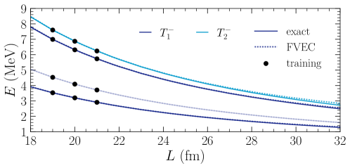
Figure 2: Negative-parity $S_{z}=1/2$ finite-volume energy spectrum of three neutrons interacting via a separable contact potential fit to reproduce the neutron-neutron scattering length $a_{nn}={-}18.9\leavevmode\nobreak\ \mathrm{fm}$. Solid lines show the exact states calculated in DVR bases with $N\leq 22$, whereas dashed lines indicate FVEC results obtained based on $N=22$ training data at three different box sizes (solid circles). A total number of $3\times 8=24$ training data were used to generate this plot, covering a subset of states from four three-dimensional cubic group multiplets.

Moreover, for truncated bases of plane-wave states as defined in Eq. (5), $S_{L,N}=\{\phi_{j}^{(L)}:j=1,{\cdot\cdot}N\}$, $D_{L,L^{\prime}}$ defines a bijection between $S_{L,N}$ and $S_{L^{\prime},N}$. Therefore, if $\psi$ and $\psi^{\prime}$ are functions expanded upon $S_{L,N}$ and $S_{L^{\prime},N}$, respectively, taking the inner product of their coefficient vectors in $\mathbb{R}^{N}$ is equivalent to considering the inner product on $\mathcal{H}$ as defined in Eq. (16). This observation, which carries over directly to the DVR basis (because that is unitary rotation of the plane-wave basis), provides a straightforward practical implementation.

An application of the method is shown in Fig. 2 for a system of three neutrons interacting via an $n=4$ super-Gaussian separable potential in the (finite-volume analog of the) ${}^{1}S_{0}$ channel, with low-energy constant $C$ is fixed to reproduce the $nn$ scattering length $a_{nn}={-}18.9\leavevmode\nobreak\ \mathrm{fm}$. Using training data from three $N=22$ DVR calculations at $L=19,20,21\leavevmode\nobreak\ \mathrm{fm}$, FVEC accurately extrapolates energy levels of low-lying negative-parity states (falling into two different representations, $T_{1}^{-}$ and $T_{2}^{-}$ of the cubic symmetry group [40]) over a large range of volumes. As emphasized numerical cost of the FVEC extrapolation is greatly reduced compared to exact calculations over the entire range of volumes shown in Fig. 2. Finite-volume eigenvector continuation is therefore an important technological advancenment that will enable the study of larger few-body systems in FV, such as for example searches for a tetraneutron resonance state.

Parts of this work have been presented at the 13th International Spring Seminar on Nuclear Physics, held in Sant’Angelo d’Ischia in May 2022. I would like to thank the organizers of that meeting for hosting a stimulating conference in a beautiful environment, and for giving me the opportunity to contribute. Moreover, I would like to thank my co-authors on the papers that this contribution is based on in part. This work was supported in part by the National Science Foundation under Grant No. PHY–2044632. This material is based upon work supported by the U.S. Department of Energy, Office of Science, Office of Nuclear Physics, under the FRIB Theory Alliance, Award No. DE-SC0013617. Computing resources for the results presented in this work were provided by the Jülich Supercomputing Center and by the Henry2 high-performance computing cluster operated by North Carolina State University.

References

References

- [1] Lüscher M 1986 Comm. Math. Phys. 104 177–206 ISSN 1432-0916
- [2] Lüscher M 1986 Comm. Math. Phys. 105 153–188 ISSN 1432-0916
- [3] Lüscher M 1991 Nucl. Phys. B 354 531–578 ISSN 0550-3213
- [4] Kreuzer S and Hammer H W 2011 Phys. Lett. B 694 424–429 (Preprint 1008.4499)
- [5] Kreuzer S and Grießhammer H W 2012 Eur. Phys. J. A 48 93 (Preprint 1205.0277)
- [6] Polejaeva K and Rusetsky A 2012 Eur. Phys. J. A 48 67 (Preprint 1203.1241)
- [7] Briceno R A and Davoudi Z 2013 Phys. Rev. D 87 094507 (Preprint 1212.3398)
- [8] Kreuzer S and Hammer H W 2013 Proceedings, 5th Asia-Pacific Conference on Few-Body Problems in Physics 2011 (APFB2011): Seoul, Korea, August 22-26, 2011 vol 54 pp 157–164
- [9] Meißner U G, Ríos G and Rusetsky A 2015 Phys. Rev. Lett. 114 091602 [Erratum: Phys. Rev. Lett.117 069902 (2016)] (Preprint 1412.4969)
- [10] Hansen M T and Sharpe S R 2015 Phys. Rev. D 92 114509 (Preprint 1504.04248)
- [11] Hammer H W, Pang J Y and Rusetsky A 2017 Journal of High Energy Physics 2017 109 ISSN 1029-8479
- [12] Hammer H W, Pang J Y and Rusetsky A 2017 Journal of High Energy Physics 2017 115 ISSN 1029-8479
- [13] Mai M and Döring M 2017 Eur. Phys. J. A 53 240 (Preprint 1709.08222)
- [14] Döring M, Hammer H W, Mai M, Pang J Y, Rusetsky A and Wu J 2018 Phys. Rev. D 97 114508 (Preprint 1802.03362)
- [15] Pang J Y, Wu J J, Hammer H W, Meißner U G and Rusetsky A 2019 Phys. Rev. D 99 074513 (Preprint 1902.01111)
- [16] Culver C, Mai M, Brett R, Alexandru A and Döring M 2020 Phys. Rev. D 101 114507 (Preprint 1911.09047)
- [17] Briceño R A, Hansen M T, Sharpe S R and Szczepaniak A P 2019 Phys. Rev. D 100 054508 (Preprint 1905.11188)
- [18] Romero-López F, Sharpe S R, Blanton T D, Briceño R A and Hansen M T 2019 Journal of High Energy Physics 2019 7 ISSN 1029-8479
- [19] Hansen M T, Romero-López F and Sharpe S R 2020 Journal of High Energy Physics 2020 47 ISSN 1029-8479 [Erratum: JHEP 02, 014 (2021)]
- [20] Müller F, Pang J Y, Rusetsky A and Wu J J 2022 Journal of High Energy Physics 2022 158 ISSN 1029-8479
- [21] Barnea N, Contessi L, Gazit D, Pederiva F and van Kolck U 2015 Phys. Rev. Lett. 114 052501 (Preprint 1311.4966)
- [22] Detmold W and Shanahan P E 2021 Phys. Rev. D 103 074503
- [23] Kirscher J, Barnea N, Gazit D, Pederiva F and van Kolck U 2015 Phys. Rev. C 92 054002 (Preprint 1506.09048)
- [24] Yaron R, Bazak B, Schäfer M and Barnea N 2022 Phys. Rev. D 106 014511 (Preprint 2206.04497)
- [25] König S, Lee D and Hammer H W 2011 Phys. Rev. Lett. 107 112001
- [26] König S, Lee D and Hammer H W 2012 Annals Phys. 327 1450–1471 ISSN 0003-4916
- [27] König S and Lee D 2018 Phys. Lett. B 779 9–15
- [28] König S 2020 Few-Body Syst. 61 20 ISSN 1432-5411
- [29] Yu H, Lee D and König S 2022 Volume dependence of charged-particle bound states (in preparation)
- [30] Dietz S, Hammer H W, König S and Schwenk A 2022 Phys. Rev. C 105(6) 064002
- [31] Yapa N and König S 2022 Phys. Rev. C 106 014309 (Preprint 2201.08313)
- [32] Klos P, König S, Hammer H W, Lynn J E and Schwenk A 2018 Phys. Rev. C 98 034004
- [33] Groenenboom G C 2001 The Discrete Variable Represenation www.theochem.kun.nl/ gerritg
- [34] Milakov M Fast integer division github.com/milakov/int_fastdiv
- [35] Elhatisari S, Epelbaum E, Krebs H, Lähde T A, Lee D, Li N, Lu B n, Meißner U G and Rupak G 2017 Phys. Rev. Lett. 119 222505 (Preprint 1702.05177)
- [36] Maschhoff K J and Sorensen D C P_ARPACK: An Efficient Portable Large Scale Eigenvalue Package for Distributed Memory Parallel Architectures www.caam.rice.edu/software/ARPACK/, github.com/opencollab/arpack-ng
- [37] Frame D, He R, Ipsen I, Lee D, Lee D and Rrapaj E 2018 Phys. Rev. Lett. 121 032501
- [38] Bonilla E, Giuliani P, Godbey K and Lee D 2022 (Preprint 2203.05284)
- [39] Melendez J A, Drischler C, Furnstahl R J, Garcia A J and Zhang X 2022 (Preprint 2203.05528)
- [40] Johnson R C 1982 Phys. Lett. B 114 147–151 ISSN 0370-2693