The future is different: Large pre-trained language models fail in prediction tasks

Abstract

Large pre-trained language models (LPLM) have shown spectacular success when fine-tuned on downstream supervised tasks. Yet, it is known that their performance can drastically drop when there is a distribution shift between the data used during training and that used at inference time. In this paper we focus on data distributions that naturally change over time and introduce four new Reddit datasets, namely the Wallstreetbets, AskScience, The Donald, and Politics sub-reddits. First, we empirically demonstrate that LPLM can display average performance drops of about 88$\%$ (in the best case!) when predicting the popularity of future posts from sub-reddits whose topic distribution changes with time. We then introduce a simple methodology that leverages neural variational dynamic topic models and attention mechanisms to infer temporal language model representations for regression tasks. Our models display performance drops of only about 40$\%$ in the worst cases (2$\%$ in the best ones) when predicting the popularity of future posts, while using only about 7$\%$ of the total number of parameters of LPLM and providing interpretable representations that offer insight into real-world events, like the GameStop short squeeze of 2021.

Keywords dynamic topic models  $\cdot$ large pre-trained models  $\cdot$ neural variational inference  $\cdot$ large language models  $\cdot$ opinion dynamics

1 Introduction

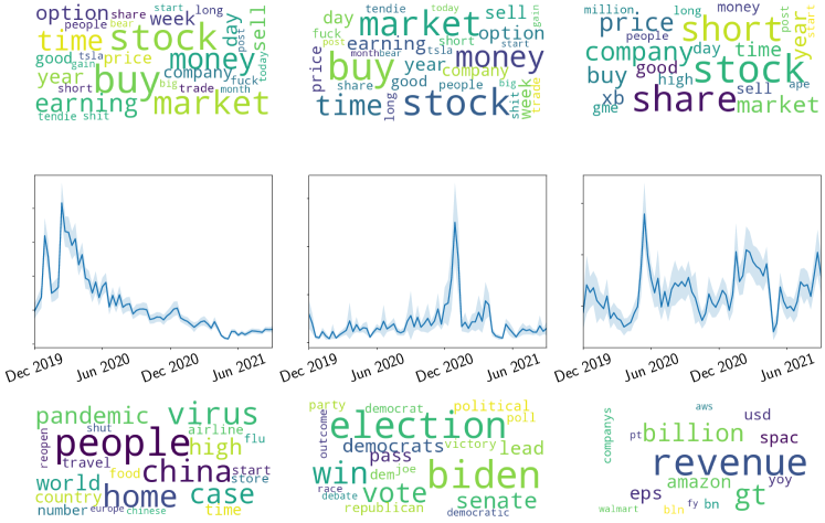
Figure 1: Dynamic features of Wallstreetbets. Top row: 30 most frequent words for all documents collected within the first, middle and last 8-week windows of the Wallstreetbets datasets. Middle row: time evolution of topic proportions from three randomly chosen topics, inferred by a neural DTM. Bottom row: top 30 words associated with each of the topics in the middle row. The figure illustrates that topic representations, as opposite to simple Bag-of-Word representations, capture (some of) the dynamic components of the dataset.

The modern natural language processing (NLP) paradigm leverages massive datasets, data-scalable (deep) attention mechanisms and minimal inductive biases Vaswani et al. (2017) in the form of large pre-trained language models (LPLM) which are subsequently fine-tuned on new learning tasks and datasets Radford et al. (2018, 2019). This approach has proven a tremendous success in supervised learning, where applications include question answering, sentiment analysis, named entity recognition and textual entailment, just to name a few (see e.g. Peters et al. (2018); Devlin et al. (2018); Liu et al. (2019); Lan et al. (2019) and Qiu et al. (2020) for a review). Yet, many recent works have also reported the strong sensitivity of LPLM to distribution shifts between the data used during training and that used at inference time Ma et al. (2019); Hendrycks et al. (2020); Zhou et al. (2021); Chawla et al. (2021). In other words, fine-tuned LPLM are known to suffer significantly at zero-shot when applied to different data domains.

In this work we focus on a particular type of natural distribution shift which arises in documents collected over long periods of time. Indeed, document collections such as magazines, academic journals, news articles and social media content not only feature trends and themes that change with time, but also employ their language differently as time evolves Danescu-Niculescu-Mizil et al. (2013). LPLM fine-tuned on documents collected up to some given time (i.e. on a given observation time window) might therefore perform poorly when evaluated in future documents, if the latter differ enough from the previously observed ones (in either content or language usage). That is, if the dataset of interest evolves in a non-stationary fashion over time. The question is then how to characterize such non-stationary features.

We introduce and study four datasets that we extract from Reddit — the news aggregator, content rating and discussion website. The goal we seek is to predict the popularity of future post, given the history (and content) of past ones. We are thus principally concerned with the two questions, namely (i) do these datasets exhibit strong enough distribution shift across time to affect the performance of LPLM, fine-tuned on the history of past posts? and, if so, (ii) how can we deal with such natural domain change problems? Each of the Reddit datasets consists, as usual, of a single sequence of document collections (i.e. each time point in the sequence consists of an aggregate of documents with a given timestamp). This practical aspect entails, in particular, that the inference of representations capturing their relevant dynamic components (i.e. the non-stationary features from above) — if at all present — should be done via low capacity models. Bayesian generative models for sequences, such as Kalman filters or Gaussian processes, are good examples well suited for such a task, and Figure 1 illustrates this point. In the first row of the figure we report the 30 most frequent words from all documents collected within the first, middle and last 8-week windows of one of our datasets, which spans about one year in total. There is no discernible change between these three time points — in this representation of the data — and one might jump to the conclusion that the dataset shows no dynamics (or that the data distribution is stationary). In the second row, however, we report how the proportions of three randomly chosen topics, inferred via a neural variational variant of Dynamic Topic Models (DTM) Blei and Lafferty (2006), changes as time evolves. Some of the dynamic features of the dataset are now evident in this representation. Note that the last row in the figure shows the top 30 words associated with each of the topics in the second row.

Our first contribution is to (empirically) show that LPLM, the likes of BERT Devlin et al. (2018) and ROBERTA Liu et al. (2019), fine-tuned on histories of past Reddit posts, display average performance drops of about 88$\%$ (in the best case!) when predicting the popularity of future posts. In sharp contrast, we shall observe that LPLM perform very well on test sets extracted from the history of past posts. This result thus responds affirmatively to our first question above.

Our second and main contribution consists of a simple methodology to deal with the kind of temporal distribution shift we observe in Reddit. Indeed, we strive to retain the expressiveness of deep neural language models (NLM) for treating the low-level word statistics composing the posts, while deploying DTM for encoding the kind of high-level document sequence dynamics shown in Figure 1. If one interprets the inferred topics as representing the domains of the dataset, their inferred dynamics can, at least in principle, account for (some aspects of) the temporal domain changes present in the dataset. Note that taking the view of topics as domains to deal with distribution shift problems has also been taken in the past, albeit in static settings Hu et al. (2014); Guo et al. (2009); Oren et al. (2019). A bit more in detail, our approach consists of mainly three components. First, we use neural variational DTM to infer the time- and document-dependent proportions of a set of latent topics that best describe the data collections. We represent this set of topics via learnable topic embeddings. Second, we deploy NLM to encode the word sequences composing the posts into sequences of contextualised word representations. Third, we modify a recently proposed attention mechanism Wang and YANG (2020) to construct temporal post representations sensitive to the temporal domain changes. These depend on both the NLM word representations of the post in question and the history of the dataset, as represented by the latent topics and their time-dependent proportions. The resulting representations can be used to predict the popularity of future posts.

Below we show our approach significantly outperforms LPLM. Indeed, our models display performance drops of only about 40$\%$ in the worst cases (2$\%$ in the best ones) when predicting the popularity of future posts, while using only about 7$\%$ of the total number of parameters of LPLM and providing interpretable representations that offer insight into real-world events, like the GameStop short squeeze of 2021.

2 Related Work

As discussed above, our methodology and the problems we tackle with it merge concepts from (i) dynamic topic models, (ii) neural models that encode both natural language and time information for supervised downstream tasks, and (iii) studies of natural distribution shifts across time and their effect on language models.

Dynamic topic models. The seminal work of Blei and Lafferty (2006) introduced the Dynamic Topic Model (DTM), which uses a state space model on the natural parameters of the distribution representing the topics, thus allowing the latter to change with time. The DTM methodology was first extended by Caron et al. (2007) to a nonparametric setting, via the correlation of Dirichlet process mixture models in time. Later Wang et al. (2012) replaced the discrete state space model of DTM with a Diffusion process, thereby extending the approach to a continuous time setting. Jähnichen et al. (2018) further extended DTM by introducing Gaussian process priors that allowed for a non-Markovian representation of the dynamics. Other recent work on dynamic topic models is that of Hida et al. (2018). Another line of research leverages neural networks to improve the performance of topic models, the so-called neural topic models Miao et al. (2016); Srivastava and Sutton (2017); Zhang et al. (2018); Dieng et al. (2020) which deploy neural variational inference Kingma and Welling (2013) for training. Within this line, the neural model of Dieng et al. (2019) represent topics as dynamic embeddings, and model words via categorical distributions whose parameters are given by the inner product between the static word embeddings and the dynamic topic embeddings. As such, this model corresponds to the dynamic extension of Dieng et al. (2020).

Dynamic language models for supervised downstream tasks. Incorporating temporal information into (neural) models of text is key to capture the constant state of flux typical of streaming text datasets, the likes of news article collections or social media content. Very early in the game, Yogatama et al. (2014) considered using temporal, non-linguistic data to condition $n$-gram language models and predict economics-related content at a given time. More recently Delasalles et al. (2019) learned, via recurrent neural models, hidden variables encoding time information, which are then used both to condition neural language models and in classification tasks. Similarly, Cvejoski et al. (2020) leveraged recurrent neural point process models to infer dynamic representations that help model both content and arrival times of Yelp reviews. Other recent work have also used both temporal and text information, but to predicting review ratings Wu et al. (2016); Cvejoski et al. (2022) instead. Yet another very recent direction involves defining protocols to update the parameters of LPLM when applied to streaming data Amba Hombaiah et al. (2021); Liska et al. (2022), with the work of Liska et al. (2022), in particular, also focusing on temporal distribution shifts.

Different from all these works, we use DTM to infer the dynamic components of our corpora, and attention mechanisms to connect them with neural language models for regression tasks.

Natural distribution shifts across time in NLP. WILDS, the benchmark introduced by Koh et al. (2021), is a very recent dataset collection which explores different types of real-world distribution shifts. Section 8 in Koh et al. (2021) focus particularly on distribution shifts in NLP and we refer the reader to it for additional details and references. Additional to these are the aforementioned works which use topic models in static settings, to tackle domain change problems Hu et al. (2014); Guo et al. (2009); Oren et al. (2019), as well as those works which report performance drops of LPLM under distribution shifts Ma et al. (2019); Hendrycks et al. (2020); Zhou et al. (2021); Chawla et al. (2021). Interestingly enough, WILDS includes in Appendix F a section about temporal distributions shift for review data. Nevertheless, they report only modest performance drops. We do not find these results surprising, for review data typically deals with items (e.g. products, restaurants, etc) whose basic features change moderately with time.

To the best of our knowledge our work is the first to present a NLP dataset displaying temporal distribution shifts on which the perfomance of LPLM drops to a significant degree.

3 Model

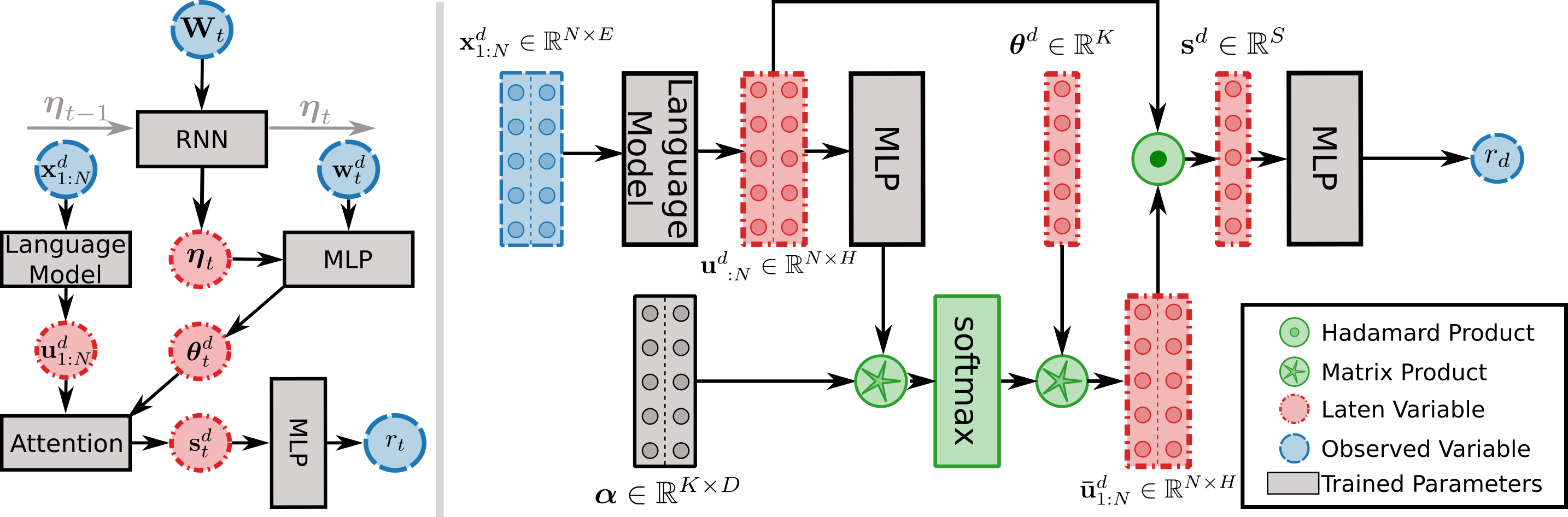
Figure 2: Left: D-TAM-GRU model. The input to the model is the document’s word sequence and BoW representation, the output is a continuous label. The model consists of four components: (i) the DTM, (ii) the NLM encoder, (iii) the attention module and (iv) a regressor module, which takes the output from the attention module and predicts a label. Right: Detailed view of the Attention Module. This module takes as input the document’s word representations from the NLM and the topic proportion from the DTM.

In this section we propose a simple methodology to deal with a class of distribution shift that naturally arises in corpora collected over long periods of time. Suppose we are given an ordered collection of corpora $\mathcal{D}=\{D_{1},D_{2},\dots,D_{T}\}$, so that the $t$th corpus $D_{t}$ is composed of $N_{t}$ documents (Reddit posts), all received within the $t$th time window. Let the $d$th document in $D_{t}$ be defined by the tuple $(\mathbf{w}_{t,d},\mathbf{X}_{t,d},r_{t,d})$, where $\mathbf{w}_{t,d}$ denotes the Bag-of-Words (BoW) representation of the document, $\mathbf{X}_{t,d}=(\mathbf{x}^{t,d}_{1},\dots,\mathbf{x}^{t,d}_{M})$ denotes the sequence of words comprising the document and $r_{t,d}$ labels the document’s rating. Similarly, let $\mathbf{W}_{t}$ denote the BoW representation for the entire document set within $D_{t}$. Given a new document $d^{\prime}$ at time $T+1$ — that is, given $\mathbf{X}_{T+1,d^{\prime}}$, $\mathbf{w}_{T+1,d^{\prime}}$ — the task is to predict the rating $r_{t+1,d^{\prime}}$.

Our approach takes the perspective that latent topics, understood as word aggregates grouped together by means of word co-occurrence information within the corpora, can be understood as representing the domains of the dataset. To allow the distribution of topics within the documents to change with time allows, at least in principle, to model domain changes within the collection as time evolves. We shall use such temporal information to weight the importance of the words composing the new document $\mathbf{X}_{T+1,d^{\prime}}$, with respect to the topic (domain) proportions in that document, at time $T+1$, by means of an attention mechanism.

The model thus requires the introduction of two components, namely (i) a neural variational DTM and (ii) an attention module that leverages the representations obtained by both the DTM and a low-level NLM, to create a temporal Reddit post representation. The resulting representation can then be used by a neural regressor model to predict $r_{t+1,d^{\prime}}$.

In the following we introduce all the different components of the model in detail.

3.1 Neural Variational Dynamic Topic Model

Let us suppose the corpora collection $\mathcal{D}$ is described by a set of $K$ unknown topics (domains). We then assume there is a sequence of global hidden variables $\bm{\mathbf{\eta}}_{1},\dots,\bm{\mathbf{\eta}}_{T}\in\mathbb{R}^{\mbox{dim}(\eta)}$ which encodes how the topic proportions change among the corpora as time evolves (i.e. as one moves from $D_{t}$ to $D_{t+1}$). We also assume there is a local hidden variable $\bm{\mathbf{\zeta}}_{t,d}\in\mathbb{R}^{\mbox{dim}(\zeta)}$, conditioned on $\bm{\mathbf{\eta}}_{t}$, which encodes the content of the $d$th document in $D_{t}$, in terms of the $K$ topics.

Generative model. Let us denote with $\psi$ the set of parameters of our generative model. We generate the $d$th document in $D_{t}$ by first sampling the topic proportions $\bm{\mathbf{\theta}}_{t,d}\in[0,1]^{K}$ as follows

$$\bm{\mathbf{\eta}}_{t} \sim \mathcal{N}\left(\bm{\mu}^{\eta}_{\psi}(\bm{\mathbf{\eta}}_{t-1}),\delta\,\mathbf{I}\right),$$ (1)

$$\bm{\mathbf{\zeta}}_{t,d} \sim \mathcal{N}\left(\mathbf{W}^{\zeta}_{\psi}\,\bm{\mathbf{\eta}}_{t}+\mathbf{c}^{\zeta}_{\psi},\,1\right),$$ (2)

$$\bm{\theta}_{t,d} = \text{softmax}(\mathbf{f}_{\psi}^{\zeta}(\bm{\mathbf{\zeta}}_{t,d})),$$ (3)

where $\mathbf{f}_{\psi}^{\zeta}:\mathbb{R}^{\mbox{dim}(\zeta)}\rightarrow\mathbb{R}^{K}$ is neural network with parameters in $\psi$ and $\mathbf{W}_{\zeta}\in\mathbb{R}^{\mbox{ dim}(\zeta)\times\mbox{ dim}(\eta)},\mathbf{c}_{\xi}\in\mathbb{R}^{\mbox{ dim}(\zeta)}\subset\psi$ are trainable parameters. Furthermore, and just as in Deep Kalman Filters Krishnan et al. (2015), $\bm{\mathbf{\eta}}_{t}$ is Markovian and evolves under a Gaussian noise with mean $\bm{\mu}^{\eta}_{\psi}:\mathbb{R}^{\mbox{dim}(\eta)}\rightarrow\mathbb{R}^{\mbox{dim}(\eta)}$, defined via a neural network with parameters $\psi$, and variance $\delta$. The latter being a hyperparameter of the model. Finally, we choose the prior $\bm{\mathbf{\eta}}_{1}\sim\mathcal{N}(0,1)$.

Once we have $\bm{\mathbf{\theta}}_{t,d}$ we generate the corpora sequence by sampling

$$z_{t,d,n} \sim \mbox{Categorical}(\bm{\theta}_{t,d}),$$ (4)

$$w_{t,d,n} \sim \mbox{Categorical}(\bm{\beta}_{z_{t,d,n}}),$$ (5)

where $z_{t,d,n}$ is the time-dependent topic assignment for $w_{t,d,n}$, which labels the $n$th word in document $d\in D_{t}$, and $\bm{\beta}\in\mathbb{R}^{K\times V}$ is a learnable topic distribution over words. We define the latter as

$$\bm{\beta}=\mbox{softmax}(\bm{\mathbf{\alpha}}\otimes\bm{\mathbf{\rho}}),$$ (6)

with $\bm{\mathbf{\alpha}}\in\mathbb{R}^{K\times E},\bm{\mathbf{\rho}}\in\mathbb{R}^{V\times E}$ learnable topic and word embeddings, respectively, for some embedding dimension $E$, and $\otimes$ denoting tensor product.

Inference model. We approximate the true posterior distribution of the hidden variables with a variational (and structured) posterior of the form

$$q_{\varphi}(\bm{\mathbf{\eta}}_{t},\bm{\mathbf{\zeta}}_{t,d}|\mathbf{w}_{t,d},\mathbf{W}_{1:T})=\prod_{t}^{T}q_{\varphi}(\bm{\mathbf{\eta}}_{t}|\bm{\mathbf{\eta}}_{1:t-1},\mathbf{W}_{1:T})\times\prod_{d}^{N_{t}}q_{\varphi}(\bm{\mathbf{\zeta}}_{t,d}|\mathbf{w}_{t,d},\bm{\mathbf{\eta}}_{t})$$ (7)

where $\mathbf{W}_{1:T}=(\mathbf{W}_{1},\dots,\mathbf{W}_{T})$ is the ordered sequence of BoW representations for the corpus collection and $\varphi$ labels the variational parameters. The posterior distribution over the local variables is chosen to be Gaussian

$$q_{\varphi}(\bm{\mathbf{\zeta}}_{t,d}|\mathbf{w}_{t,d},\bm{\mathbf{\eta}}_{t})=\mathcal{N}(\bm{\mathbf{\mu}}^{\zeta}_{\varphi}[\mathbf{w}_{t,d},\bm{\mathbf{\eta}}_{t}],\bm{\mathbf{\sigma}}^{\zeta}_{\varphi}[\mathbf{w}_{t,d},\bm{\mathbf{\eta}}_{t}]),$$ (8)

with $\bm{\mathbf{\mu}}^{\zeta}_{\varphi}$ and $\bm{\mathbf{\sigma}}^{\zeta}_{\varphi}$ neural networks with parameter $\varphi$. Likewise, the posterior distribution over the global variables is also Gaussian, but now depends not only on the latent variables at time $t-1$, but also on the entire sequence of BoW representations $\mathbf{W}_{1:T}$. Explicitly we write

$$q_{\varphi}(\bm{\mathbf{\eta}}_{t}|\bm{\mathbf{\eta}}_{t-1},\mathbf{W}_{1:T})=\mathcal{N}(\bm{\mathbf{\mu}}^{\eta}_{\varphi}[\bm{\mathbf{\eta}}_{t-1},\mathbf{h}^{\eta}_{T}],\bm{\mathbf{\sigma}}^{\eta}_{\varphi}[\bm{\mathbf{\eta}}_{t-1},\mathbf{h}^{\eta}_{T}]),$$ (9)

where $\bm{\mathbf{\mu}}^{\eta}_{\varphi},\bm{\mathbf{\sigma}}^{\eta}_{\varphi}$ are too given by neural networks and $\mathbf{h}^{\eta}_{t}$ is a recurrent representation encoding the sequence $\mathbf{W}_{1:T}$. Indeed,

$$\mathbf{h}^{\eta}_{t}=g^{\eta}_{\varphi}(\mathbf{W}_{t},\mathbf{h}^{\eta}_{t-1}),$$ (10)

with $g_{\varphi}$ a neural model for sequence processing (like e.g. a GRU Cho et al. (2014)). Figure 2 illustrates the architecture of the complete model.

Training objective. To optimize the DTM parameters $\{\psi,\varphi\}$ we minimize the variational lower bound on the logarithm of the marginal likelihood $p_{\psi}(w_{t,d,n}|\bm{\mathbf{\beta}})$. Following standard methods Bishop (2006), the latter can readily be shown to be

$$\mathcal{L}[\bm{\beta},\psi,\varphi]=\sum_{t=1}^{T}\sum_{d=1}^{N_{t}}\Bigg{(}\mathbb{E}_{\left\{\bm{\mathbf{\zeta}}_{t,d},\bm{\mathbf{\eta}}_{t}\right\}}\Big{\{}\log p_{\psi}(\mathbf{w}_{t,d}|\bm{\beta},\bm{\mathbf{\zeta}}_{t,d},\bm{\mathbf{\eta}}_{t})-\mbox{KL}\left[q_{\varphi}(\bm{\mathbf{\zeta}}_{t,d}|\mathbf{w}_{t,d},\bm{\mathbf{\eta}}_{t});p_{\psi}(\bm{\mathbf{\zeta}}_{t,d}|\bm{\mathbf{\eta}}_{t})\right]\Big{\}}\Bigg{)}\\ -\mbox{KL}\left[q_{\varphi}(\bm{\mathbf{\eta}}_{1}|\mathbf{W}_{1:T});p(\bm{\mathbf{\eta}}_{1})\right]-\sum_{t=2}^{T}\mbox{KL}\left[q_{\varphi}(\bm{\mathbf{\eta}}_{t}|\bm{\mathbf{\eta}}_{1:t-1},\mathbf{W}_{1:T});p_{\psi}(\bm{\mathbf{\eta}}_{t}|\bm{\mathbf{\eta}}_{t-1})\right],$$ (11)

where KL labels the Kullback-Leibler divergence and $\bm{\mathbf{\beta}}$ is given in equation (6).

3.2 Neural Topic Attention Model

Given a document $d$, composed of the word sequence $\mathbf{x}_{1},\dots,\mathbf{x}_{M}$, the task is to predict its rating $r_{d}$. One straightforward approach to this problem is to consider a (deep) neural language model to infer contextualized word representations of the form

$$\mathbf{u}_{1},\mathbf{u}_{2},\dots,\mathbf{u}_{M}=s_{\rho}(\mathbf{x}_{1},\mathbf{x}_{2},\dots,\mathbf{x}_{M}),$$ (12)

where $s_{\rho}$ is any neural sequence processing model (as e.g. a GRU Cho et al. (2014) or BERT model) with parameters $\rho$.

With the representations $\mathbf{u}_{1},\mathbf{u}_{2},\dots,\mathbf{u}_{M}$ at hand one can define a summary representation $\mathbf{s}_{d}$ (by e.g. averaging over the $\mathbf{u}$’s or using the CLS token of BERT-like models) and use it as input to a neural regressor $\mathbf{f}^{r}_{\rho}$ (also with parameters $\rho$) to predict $r_{d}$. Yet, if the document $d$ is received at time $T+1$, i.e. out of the observation window on which the parameter $\rho$ was optimised, and if the dataset in question displays temporal domain changes, we might expect our simple model to underperform.

Here we use the DTM of section 3.1, which is assumed to model the domain changes in the corpora, to define a temporal summary representation sensible to the natural distribution shifts of the dataset. Indeed, we follow Wang and YANG (2020) and use an attention mechanism to construct $\mathbf{s}_{d}$ as follows

$$\mathbf{s}_{t,d}=\sum_{j}^{M}\sum_{i}^{K}(\theta_{t,d}^{i}-\delta)\,\text{softmax}(\text{MLP}(\mathbf{u}_{j})^{T}\cdot\bm{\mathbf{\alpha}}_{i})\,\odot\mathbf{u}_{j},$$ (13)

where the softmax function is taken with respect to the word sequence, the $\bm{\mathbf{\alpha}}_{i}$ label the set of $K$ global topic embeddings and the $\theta_{t,d}$ denote the time- and document-dependent topic proportions, as defined in Eq. 3.

It follows that the proposed document representation is nothing but the sum of the projections of each of the document’s word representations onto topic space, weighted by the time-dependent topic proportions of each dimension. It can also be understood as an attentive representation in which each word is queried by the weighted topics.

In what follows we let $\mathbf{s}_{\rho}$ be modeled by a GRU network Cho et al. (2014) and name the model thus defined D-TAM-GRU. Our proposed framework is shown in Figure 2.

3.3 Training Objective

To optimize the complete set of model parameters $\{\psi,\varphi,\bm{\mathbf{\rho}}\}$ we minimize the objective

$$\mathcal{L}=\mathcal{L}_{TM}[\bm{\beta},\psi,\varphi]+\alpha_{y}\mathcal{L}_{r}[\bm{\rho}],$$ (14)

where $\mathcal{L}_{TM}$ denotes the DTM loss (defined in Eq. 11) and $\mathcal{L}_{r}$ denotes the regression loss. The latter is defined as the root-mean-squared error between the target rating $r_{d}$ and the prediction of a regressor model, that is

$$\mathcal{L}_{r}[\bm{\rho}]=\text{RMSE}(r_{d},\mathbf{f}^{r}_{\rho}\left(\mathbf{s}_{d}\right)),$$ (15)

with $\mathbf{f}^{r}:\mathbb{R}^{\mbox{dim}(s)}\rightarrow\mathbb{R}$ a neural network and $\mathbf{s}_{d}$ defined by Eq. 13.

3.4 Prediction

In order to predict the rating $r_{T+N,d}$ of a new document, $N$ steps into the future, given its word sequence $\mathbf{X}_{T+N,d}$, we rely on the generative process of our model albeit conditioned on the past. Essentially one must generate Monte Carlo samples from the posterior distribution and propagate the global latent representations into the future with the help of the prior transition function Eq,. 1. This procedure is depicted on the conditional predictive distribution (for a single step) of our model

$$p(r_{T+1,d}|\mathcal{D},\mathbf{X}_{T+1,d})=\int p(r_{T+1,d}|\bm{\mathbf{\eta}}_{T+1},\bm{\mathbf{\zeta}}_{T+1,d},\mathbf{X}_{T+1,d})\\ \times p(\bm{\mathbf{\zeta}}_{T+1,d}|\bm{\mathbf{\eta}}_{T+1})p(\bm{\mathbf{\eta}}_{T+1}|\bm{\mathbf{\eta}}_{T})p(\bm{\mathbf{\eta}}_{1:T}|\mathcal{D})d\bm{\mathbf{\eta}}_{1:T+1}d\bm{\mathbf{\zeta}}_{T+1,d},$$ (16)

where $p(\bm{\mathbf{\eta}}_{1:t}|\mathcal{D})$ is the exact posterior over the dynamical global variables, which we approximate with our variational expression Eq. 9, and where

$$p(r_{T+1,d}|\bm{\mathbf{\eta}}_{T+1},\bm{\mathbf{\zeta}}_{T+1,d},\mathbf{X}_{T+1,d})=\delta(r_{T+1,d}-\mathbf{f}_{\rho}^{r}(\mathbf{s}_{T+1,d}[\bm{\mathbf{\eta}}_{T+1},\bm{\mathbf{\zeta}}_{T+1,d},\mathbf{X}_{T+1,d}])),$$ (17)

with $\mathbf{f}_{\rho}^{r}$ the neural regressor, $\mathbf{s}_{T+1,d}$ defined in Eq. equation (13) and $\delta$ the Dirac delta function.

Table 1: In-distribution results (Results in Test set defined in up-to-date data), which violate causality, we use information from the future to predict the past. For each of the number of topics column we underline the best models within and with boldface the best models overall.

	Model	R2$\uparrow$			PPL-DC$\downarrow$
		25	50	100	25	50	100
AskScience	MLP	0.0007
	BERT	0.0712
	RoBERTa	0.0484
	TAM-GRU	0.0053	0.0555	0.0449	1615	1616	1561
	TAM-BERT	0.0103	0.0967	0.0867	1462	1647	1549
	TAM-RoBERTa	-0.0175	-0.0169	0.0295	3290	1770	1612
	D-ST	-0.0175	-0.0138	-0.0175	2147	1745	1691
	D-TAM-GRU	0.0387	0.0386	0.0397	1795	1813	1723
Politics	MLP	0.6278
	BERT	0.6820
	RoBERTa	0.7306
	TAM-GRU	0.7063	0.6918	0.6847	1857	2007	2022
	TAM-BERT	0.7268	0.6639	0.6802	2075	1986	1997
	TAM-RoBERTa	-0.0191	0.6329	0.6305	3548	1998	1976
	D-ST	0.3370	0.3631	0.2372	2157	2147	2014
	D-TAM-GRU	0.6705	0.6892	0.6836	2149	2118	2051
The Donald	MLP	0.4162
	BERT	0.6674
	RoBERTa	0.5290
	TAM-GRU	0.3493	0.3772	0.3195	1887	1873	1893
	TAM-BERT	0.5965	0.6537	0.6659	2138	1895	2009
	TAM-RoBERTa	0.5992	0.4878	0.5906	2195	2066	2073
	D-ST	-0.0014	-0.0015	-0.0012	2162	2121	1986
	D-TAM-GRU	0.4374	0.4342	0.4302	2186	2125	2143
Wallstreetbets	MLP	0.5862
	BERT	0.6850
	RoBERTa	0.5484
	TAM-GRU	0.4961	0.5134	0.5037	1373	1436	1390
	TAM-BERT	0.5253	0.4057	0.8293	1341	1360	1325
	TAM-RoBERTa	-0.0084	0.5994	0.0218	1539	1474	1355
	D-ST	-0.0038	-0.0022	0.1823	1693	1497	1566
	D-TAM-GRU	0.4989	0.5340	0.5066	1993	1466	1541

4 Dataset and Experimental Setup

Table 2: Datasets’ statistics.

	AskScience	Politics	The Donald	Wallstreetbets
maximum doc. size	120	150	200	500
# of time steps train/prediction	25/20 (months)	124/20 (weeks)	93/25 (weeks)	72/25 (weeks)
# of train/test/prediction docs.	11 259/1 408/12 217	25 432/3 179/3 214	37 140/4 643/10 000	28 297/3 538/9 882
vocabulary size - TM/LM	4 968/9 108	5 000/12 473	4 996/22 380	4 998/23 438
start-end train/prediction time	01.01.18-01.01.20/30.09.21	01.01.19-11.05.21/30.09.21	01.01.2018-06.10.19/29.02.20	01.01.20-13.05.21/30.09.21

In this sections we present detailed information about our proposed Reddit dataset for temporal distribution shifts analysis. Next, we describe the experimental setup that we use to train and evaluate the models and introduce the baselines we compare against.

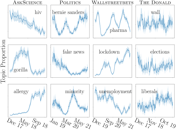
Figure 3: Time evolution of topics’ proportion. The time series are obtained by taking the mean and two standard deviations of the activity $\theta_{k}$ of topic $k$ in all the documents for a given time step $t$. We present three randomly picked topics for each dataset. One could immediately notice that there is almost no dynamics for the The Donald dataset.

4.1 Dataset

In this work we propose a new Reddit dataset for temporal distribution shifts analysis. Reddit is a news aggregator, content rating and discussion website. Users can post content on the site, like images, text links and videos, which are rated and commented by other users. The posts which are called submissions are organized by subject in groups or subreddits. According to Semrush, as of March 2022 Reddit is ranked as the 9th most visited website worldwide. We crawled the posts for the AskScience, Politics, The Donald and the Wallstreetbets subreddits. The AskScience is a subreddit in which science questions are posted and answered. Politics is a subreddit where news and politics in the U.S. are discussed. The Donald was a subreddit where supporters of former U.S. president Donald Trump were initiating discussions. This subreddit was banned in June 2020 for violating Reddit rules. Lastly, the Wallstreetbets is a subreddit where stock trading is discussed. This subreddit played a major role in the GameStop short squeeze that caused losses for some U.S. firms in early 2021.

4.2 Preprocessing

Crawled raw submission are preprocessed as follows. First, we remove all the submissions that are created by the automated system (e.g. when the author’s name is AutoModerator), as well as submissions that have less than 20 words, and submissions containing text different than English. Next, we discretise the time interval into weekly time points (AskScience in monthly time steps) and randomly sub-sample 500 data points for each time point (1000 data points for AskScience). We also use different preprocessing for the NLE and the DTM.

DTM Preprocessing. We remove emojis, urls stop words, punctuation and spaces, and we lemmatize the words. We also remove all the words that appear in less than 5 documents, and we take the first 5000 words (in ascending order wrt. word frequency) as vocabulary, which we then use to create BoW vectors for each document.

NLM Preprocessing. Urls, spaces and other characters like HTML tags are removed and a maximum post length is defined (see Table 2 for details). Also all posts that have more than 50 000 comments are removed, and the target variable (i.e. the rating $r$ or number of comments) is scaled to have values between 0 and 1.

Time Window and Out-of-Distribution Selection. After pre-processing, we first split each of the datasets into the up-to-date and prediction datasets. We create such a distinction to study temporal distribution shifts in the dataset. Specifically, we take the last 20 time points as prediction (Out-of-distribution data) and the rest for the up-to-date posts (In-Distribution data). In this way we ensure that we do not train on documents that come from the future, which is what we actually want to model. That is, we do not violate causality. Likewise we ensure there is a clear distinction between past and future, which will allow us to uncover temporal distribution shifts, if present. Table 2 displays the specific timestamps which define the beginning and end of each dataset slice.

Next, we split the up-to-date submissions randomly into train, validation and test sets (80%, 10%, 10%, respectively). Additionally, to evaluate the DTM on the document completion (i.e. generalization) task, we split the documents of the test set into two halves. The first half is used as input to the topic model; the second half is used to measure the document completion perplexity.

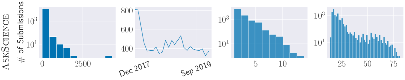
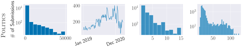
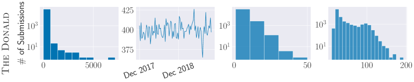
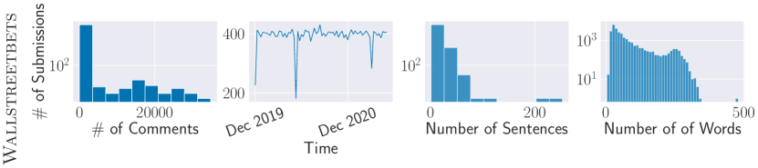
Figure 6: Reddit datasets’ statistics. In the first column are presented the histograms of the number of comments per submission. Next column, contains the number of submission per week (month in the case of AskScience). The last two columns contain the histograms of the number of sentences and number of words per submissions, respectively.

Further statistics about the Reddit dataset (like e.g. histograms of the number of comments per post, etc) can be found in Fig. 6 in the Appendix.

4.3 Baseline Models

The baseline models are introduced in order of increasing complexity. These models are generally composed of two modules, namely (i) an encoder module, which takes as input either the word sequence $\mathbf{X}_{t,d}$ or the BoW $\mathbf{w}_{t,d}$ of the document and outputs a summary representation $\mathbf{s}_{d,t}$; (ii) a regressor module, which takes as input the representation $\mathbf{s}_{d,t}$ and predicts the rating $r_{t,d}$ of the document.

The simplest baseline model we consider defines both encoder and regressor as MLPs, and takes as input the BoW representation $\mathbf{w}_{t,d}$ of the document. We name it MLP. Next we introduce baselines with attention-based models Vaswani et al. (2017) as encoder and MLPs as regressor. We use two attention-based encoder architectures:. BERT Devlin et al. (2018) and RoBERTa Liu et al. (2019). The input to these models is the word sequence $\mathbf{X}_{t,d}$ and we use their CLS embedding as input to the regressor module. The third baseline is TAM, the neural topic attention model for supervised learning proposed by Wang and YANG (2020). TAM combines topic models and NLM to produce the representation $\mathbf{s}_{d,t}$, just as in Eq. 13 above, but with static topic proportions. The original TAM version uses a GRU as NLM. We call this version TAM-GRU. We also extend this model by replacing the GRU with either BERT or RoBERTa. Accordingly we name these baselines TAM-BERT and TAM-RoBERTa, respectively. Finally, we use our DTM from section 3.1 as encoder module, and input the inferred local hidden variable $\bm{\mathbf{\zeta}}_{t,d}$ to the regressor, which here too is defined by an MLP. We name this last baseline D-ST.

4.4 Training and Evaluation Metrics

We use grid search during training to find the best hyper-parameters of each model type. All models are trained on the training subset of the up-to-date submissions, and the validation subset is used for choosing the best hyper-parameters. For all models that rely on a DTM module we use 25, 50 and 100 topics. Details regarding the values of other hyper-parameters can be found in the Appendix A.1.

We quantify the performance of our models on the prediction tasks with the coefficient of determination ($R^{2}$). Additionaly, we also evaluate the performance of the topic models, whenever this are used, by means of the predictive perplexity (PPL-P), the perplexity on document completion (PPL-DC) Rosen-Zvi et al. (2012) and the topic coherence (TC) Lau et al. (2014). Additional details about the metrics can be found in the appendix A.2. We also provide the new proposed Reddit dataset and as well as the Torch Paszke et al. (2019) implementation of the used models and scripts for downloading the data.

5 Results and Discussion

Table 3: prediction: Out-of-Distribution results which respect causality, the information of the past is used to predict the future. For each of the number of topics column we underline the best models within and with boldface the best models overall.

	Model	R2$\uparrow$			PPL-P$\downarrow$			TC$\uparrow$
		25	50	100	25	50	100	25	50	100
Askscience	MLP	0.011$\pm$0.012
	BERT	-1.029$\pm$0.756
	RoBERTa	0.105$\pm$0.158
	TAM-GRU	0.075$\pm$0.096	0.150$\pm$0.118	0.164$\pm$0.141	1525	1609	1502	-0.32	-0.38	-0.35
	TAM-BERT	0.054$\pm$0.103	0.134$\pm$0.171	0.154$\pm$0.170	1370	1257	1348	-0.06	-0.14	-0.23
	TAM-RoBERTa	-0.019$\pm$0.008	-0.019$\pm$0.008	0.092$\pm$0.099	2668	1867	1620	-0.45	-0.36	-0.41
	D-ST	0.008$\pm$0.030	-0.010$\pm$0.010	-0.006$\pm$0.008	1914	1867	2031	-0.34	-0.45	-0.59
	D-TAM-GRU	0.152$\pm$0.105	0.196$\pm$0.175	0.173$\pm$0.161	1904	1844	1752	-0.27	-0.39	-0.50
Politics	MLP	-2.507$\pm$8.977
	BERT	-4.569$\pm$14.48
	RoBERTa	0.087$\pm$0.352
	TAM-GRU	0.194$\pm$0.255	-0.017$\pm$0.017	-0.421$\pm$1.079	1486	1486	1877	-0.52	-0.63	-0.27
	TAM-BERT	-0.031$\pm$0.077	-0.091$\pm$0.047	-0.362$\pm$0.885	2126	1992	1759	-0.58	-0.56	0.07
	TAM-RoBERTa	-0.091$\pm$0.047	0.054$\pm$0.227	0.008$\pm$0.408	3368	2081	2109	-0.36	-0.63	-0.56
	D-ST	-0.072$\pm$0.216	-0.191$\pm$0.127	-0.178$\pm$0.291	2394	2425	2248	-0.26	-0.50	-0.36
	D-TAM-GRU	-0.016$\pm$0.015	0.408$\pm$0.221	0.129$\pm$0.169	2336	2250	2288	0.01	-0.21	-0.31
The Donald	MLP	-0.009$\pm$0.010
	BERT	-0.047$\pm$0.029
	RoBERTa	0.110$\pm$0.258
	TAM-GRU	0.052$\pm$0.226	0.084$\pm$0.250	0.102$\pm$0.281	2199	2061	1608	-0.53	-0.63	0.03
	TAM-BERT	0.079$\pm$0.292	0.094$\pm$0.286	-0.116$\pm$0.072	2048	1594	2263	-0.12	-0.12	0.05
	TAM-RoBERTa	-0.116$\pm$0.072	-0.036$\pm$0.024	-0.032$\pm$0.203	6331	1870	2041	-0.29	-0.34	-0.42
	D-ST	-0.011$\pm$0.011	-0.012$\pm$0.011	-0.011$\pm$0.010	2144	2105	1858	0.03	-0.48	-0.52
	D-TAM-GRU	0.045$\pm$0.181	0.048$\pm$0.209	0.085$\pm$0.251	2131	2183	2064	-0.04	-0.34	-0.29
Wallstreetbets	MLP	0.481$\pm$0.506
	BERT	-2.044$\pm$8.304
	RoBERTa	-0.002$\pm$0.009
	TAM-GRU	0.318$\pm$0.253	-0.017$\pm$0.015	-1.913$\pm$7.801	1486	1657	1271	-0.40	-0.59	-0.29
	TAM-BERT	-0.016$\pm$0.015	0.494$\pm$0.120	0.042$\pm$0.054	1232	1350	1171	0.17	-0.32	0.14
	TAM-RoBERTa	-0.014$\pm$0.025	-0.008$\pm$0.005	-0.280$\pm$1.139	2384	1543	1518	-0.39	-0.57	-0.51
	D-ST	0.510$\pm$0.296	-0.008$\pm$0.006	0.376$\pm$0.165	2491	1782	1576	-0.07	-0.30	-0.44
	D-TAM-GRU	-0.016$\pm$0.015	0.503$\pm$0.291	0.524$\pm$0.199	2160	1700	1583	0.00	-0.33	-0.22

In this section we discuss our results on the task of predicting the popularity of future submissions (posts) on the Reddit platform, by predicting the number of comments the submissions will receive. As explained above, this task is defined by training all models on the up-to-date submission set and evaluating them on the prediction set, which consists of submissions received in the future.

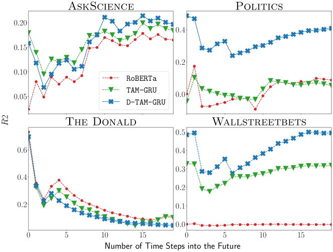
Figure 4: Cumulative average $R2$ score for each time step into the future obtained by using the predictions of the best transformer, the best static TAM and the best dynamic TAM models. Our models perform in all the datasets better than the static ones, except in the The Donald dataset which exhibits more stationary behavior, and in this case our model is not suitable. The rolling window size for calculating the cumulative average is 5 time steps.

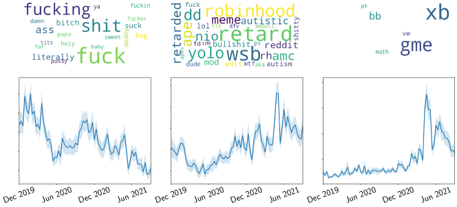
Figure 5: Evolution of topic proportion in the Wallstreetbets dataset. Topics showing community culture (profane jargon) and the behavior of the population during to the "GameStop" short squeeze event.

One of the key takeaways of the present work is to highlight that LPLM, fine-tuned on the up-to-date submissions, fail at predicting the popularity of future posts. Too see this let us first examine the results in Table 1, which show the performance of all models, evaluated on the test subset of the up-to-date submissions set. That is, Table 1 shows the In-distribution results. Note how LPLM provide the best results in all subreddits, yielding $R^{2}$ scores which are 20% to 30% higher than the dynamic models, including our D-TAM-GRU. In contrast, Table 3 shows the Out-of-Distribution results, that is, the results of all models evaluated on the prediction set. Comparing the performance of LPLM on the In-Distribution set against their performance on the Out-of-Distribution set, we observe performance drops of about 88$\%$ (in the best case!). LPLM thus fail at predicting the popularity of future posts, and we understand these findings as being consequence of temporal distributions shifts between the up-to-date and prediction sets.

The second important observation we can make from Table 3 is that, with the exception of those results in The Donald subreddit, D-TAM-GRU not only outperforms all LPLM, but also displays performance drops of only about 40$\%$ in the worst case (2$\%$ in the best ones) when predicting the popularity of future posts. Thus, our simple methodology does in fact help dealing with the temporal distributions shifts of the Reddit dataset.

To understand why D-TAM-GRU performs as it does on The Donald subreddit, we studied the dynamic features inferred by our DTM on all subreddits. Figure 3 displays the time series for the topic proportions of three randomly selected topics from each dataset. Note how the topics exhibit a different range of dynamic behavior, accounting for seasonality, trendiness and bursty as well as simply random behavior. As a whole, the ability of the model to leverage such dynamic information in the prediction task strongly depends on the nature of these dynamical patterns, as well as the overall weight obtained by the topic attention mechanism. Indeed, one requires enough relevant topics with dynamical information. In what can be thought of as a kind of distributed signal-to-noise ratio, we speculate that in order for the prediction capabilities of NLMs to be improved by our approach, the dataset at hand must be such that there are enough topics with non-stationary behavior, i.e. topics that exhibit a distribution change over time, and that such topics are important for the prediction task, above other topics with stationary dynamical behavior (i.e. no change in time). The Donald dataset shows qualitative behavior that is overall stationary, as the topic proportions present mainly noisy behavior, which explains why D-TAM-GRU exhibits performance drops as large as those of the LPLM.

Finally, our ablation study also shows that (static) topic attention models expand the capabilities of LPLM. See Table 3 and Figure 4. These findings comply with results in the literature, which indicate that topic models largely improve model performance under distribution shifts Hu et al. (2014); Guo et al. (2009); Oren et al. (2019).

Interpretability and Wallstreetbets. An added advantage of our model is the interpretable character of the representations inferred by our DTM, as we have seen in Figure 5. The Wallstreetbets subreddit has become a success story when it comes to the power the Web has to impact society, as retail investors organized themselves in the platform to create major shifts in the stock market, thereby playing a major role in short squeeze of the "GameStop" stock (an American video game retailer). This event can be directly observed in Fig. 5-right, where the model inferred a rapid increase in the importance of a topic about “gme" (ticker value of the “GameStop" stock), previous to the sudden increase of the stock price by January 28, 2021. Now, due to the rapid increase of the stock price, some brokerages such as “Robinhood" halted trading. The reaction of the community to this decision can also be observed in the rise of the topic shown in Fig.  5-middle, in which“Robinhood" is paired with derogatory jargon. New insights into the behavior of the population are uncovered by our model too. Fig. 5-left shows how profane-related topic decays in importance with time, which means that the language used by the Wallstreetbets subreddit community is shifting.

Beyond these qualitative results, the ability of our model to predict the popularity of posts, allows us to quantify the impact of several topics in the platform, as well as to predict popularity shifts within the user population. As Wallstreetbets continues to gain ground with retail investors, our methodology opens a window to quantitatively study possible future rises in the popularity of futures stocks in the Reddit platform.

6 Conclusion

In this work we studied the prediction capabilities of large pre-trained language models (LPLM) and showed that, for a newly introduced dataset with rich dynamic behavior, temporal distribution shifts produce a sharp drop in the performance of these LPLM. We introduced a neural variational dynamic topic model with attention that outperforms LPLM and overcomes (some of) the difficulties created by the temporal distribution shifts. Remarkably, our models use only about 7% of the total number of parameters of LPLM and provide interpretable representations that offer insight into real-world events.

Appendix A Experimental Setup

A.1 Model Training Setup

We use grid search during training to find the best hyper-parameters for each model type. All models are trained on the training set and the validation set is used for picking the best hyper-parameters for each model type. Early stopping during training was used, where as metric for improvement is used root-mean-squared error (RMSE). For all the models the representation size that comes out from the encoder is 128, except for the transformer models where the size is 768. The encoder size for all the model is MLP with two hidden layers of size 256 and we use Dropout Srivastava et al. [2014] with probability of 0.3. For the models that combine topic model and transformer as language model we use two optimizer, one for the topic model and regressor and the second one for the transformer. This is done because we use already pre-trained transformers models that only needed to be finetuned with small learning rate. SGD Kiefer and Wolfowitz [1952] was used as first optimizer and AdamW Loshchilov and Hutter [2017] for training the transformers. In the next we will describe for all the models the parameter grid used in the grid search algorithm: (1) MLP: learning rate $[0.001,0.0005]$; batch size $[32,128]$; regressor size [linear layer, two hidden layers of size 256]; max number of epochs is $200$; (2) BERT, ALBERT and RoBERTa: learning rate $[1\mathrm{e}^{-5},1\mathrm{e}^{-6}]$; batch size $[8,16]$; regressor size two hidden layers of size 256; max number of epochs is $20$; (3) TAM-GRU: learning rate $[0.001,0.0005]$; batch size $[32,64,128]$; regressor size two hidden layers of size 256; max number of epochs is $200$; (4) ATM-<TRANSFORMER>: learning rate $[(1\mathrm{e}^{-3},1\mathrm{e}^{-6}),(5\mathrm{e}^{-4},1\mathrm{e}^{-6})]$; batch size $[16,32]$; (5) D-ST and D-TAM-GRU: learning rate $[0.001,0.0005]$; batch size $[32,128]$; for inference of the global variable $\bm{\mathbf{\eta}}_{t}$ (see Equation (9)) we use LSTM Hochreiter and Schmidhuber [1997] with 4 layers with hidden size 400 and dropout 0.3; the transition function of the global variable (see Equation (1)) is MLP with two hidden layers of size 64; the size of the $\bm{\mathbf{\eta}}_{t}$ is equal to the number of topics. All the models that have $\alpha_{y}$ we look in $[1,100,500,1000]$ and values for $\delta$ we take $0.2,0.1,0.005$ for the 25, 50 and 100 topics respectively. Pre-traind GloVE Pennington et al. [2014] word embeddings are used for the word representations $\bm{\mathbf{\rho}}$ in the topic model and as word embeddings in the case when the GRU is used as LM.

A.2 Metrics

In order to quantify the performance of our models, we first focus on two aspects, namely its prediction capabilities and its ability to generalize to unseen data. To test how well our models perform on a prediction task we compute the predictive perplexity (PPL-P). To our knowledge this metric does not appear explicitly in the dynamic topic model literature, therefore we define this metrics as

$$\text{PPL-P}=\text{exp}\Big{\{}\mathbb{E}_{p_{\psi}(\bm{\mathbf{\Gamma}}_{T+1}|\bm{\mathbf{\Gamma}}_{T})}\mathbb{E}_{q_{\varphi}(\bm{\mathbf{\Gamma}}_{1:T}|\mathbf{W}_{1:T})}\Big{\{}\log p_{\psi}(\mathbf{W}_{T+1}|\bm{\mathbf{\Gamma}}_{T+1})\Big{\}}\Big{\}},$$ (18)

where $\bm{\mathbf{\Gamma}}_{t}$ labels the set $\{\bm{\mathbf{\eta}}_{t},\bm{\mathbf{\zeta}}_{t,d}\}$.

In order to test the generalization capabilities we use three metrics namely, perplexity (PPL-DC) on document completion, topic coherence (TC) and coefficient of determination ($R^{2}$). The document completion PPL is calculated on the second half of the documents in the test set, conditioned on their first half Rosen-Zvi et al. [2012]. The TC is calculated by taking the average pointwise mutual information between two words drawn randomly from the same topic Lau et al. [2014] and measures the interpretability of the topic.

A.3 Dataset Statistics

References

- Amba Hombaiah et al. [2021] S. Amba Hombaiah, T. Chen, M. Zhang, M. Bendersky, and M. Najork. Dynamic language models for continuously evolving content. In Proceedings of the 27th ACM SIGKDD Conference on Knowledge Discovery & Data Mining, pages 2514–2524, 2021.
- Bishop [2006] C. M. Bishop. Pattern recognition and machine learning. springer, 2006.
- Blei and Lafferty [2006] D. M. Blei and J. D. Lafferty. Dynamic topic models. In Proceedings of the 23rd international conference on Machine learning, pages 113–120, 2006.
- Caron et al. [2007] F. Caron, M. Davy, and A. Doucet. Generalized polya urn for time-varying dirichlet process mixtures. In Proceedings of the Twenty-Third Conference on Uncertainty in Artificial Intelligence, UAI’07, page 33–40, Arlington, Virginia, USA, 2007. AUAI Press. ISBN 0974903930.
- Chawla et al. [2021] S. Chawla, N. Singh, and I. Drori. Quantifying and alleviating distribution shifts in foundation models on review classification. In NeurIPS 2021 Workshop on Distribution Shifts: Connecting Methods and Applications, 2021. URL https://openreview.net/forum?id=OG78-TuPcvL.
- Cho et al. [2014] K. Cho, B. Van Merriënboer, D. Bahdanau, and Y. Bengio. On the properties of neural machine translation: Encoder-decoder approaches. arXiv preprint arXiv:1409.1259, 2014.
- Cvejoski et al. [2020] K. Cvejoski, R. J. Sánchez, B. Georgiev, C. Bauckhage, and C. Ojeda. Recurrent point review models. In 2020 International Joint Conference on Neural Networks (IJCNN), pages 1–8, 2020. doi: 10.1109/IJCNN48605.2020.9206768.
- Cvejoski et al. [2022] K. Cvejoski, R. J. Sánchez, C. Bauckhage, and C. Ojeda. Dynamic review-based recommenders. In P. Haber, T. J. Lampoltshammer, H. Leopold, and M. Mayr, editors, Data Science – Analytics and Applications, pages 66–71, Wiesbaden, 2022. Springer Fachmedien Wiesbaden.
- Danescu-Niculescu-Mizil et al. [2013] C. Danescu-Niculescu-Mizil, R. West, D. Jurafsky, J. Leskovec, and C. Potts. No country for old members: User lifecycle and linguistic change in online communities. In Proceedings of the 22nd International Conference on World Wide Web, page 307–318, New York, NY, USA, 2013. Association for Computing Machinery. ISBN 9781450320351.
- Delasalles et al. [2019] E. Delasalles, S. Lamprier, and L. Denoyer. Dynamic neural language models. In T. Gedeon, K. W. Wong, and M. Lee, editors, Neural Information Processing, pages 282–294, Cham, 2019. Springer International Publishing.
- Devlin et al. [2018] J. Devlin, M.-W. Chang, K. Lee, and K. Toutanova. Bert: Pre-training of deep bidirectional transformers for language understanding. arXiv preprint arXiv:1810.04805, 2018.
- Dieng et al. [2019] A. B. Dieng, F. J. Ruiz, and D. M. Blei. The dynamic embedded topic model. arXiv preprint arXiv:1907.05545, 2019.
- Dieng et al. [2020] A. B. Dieng, F. J. Ruiz, and D. M. Blei. Topic modeling in embedding spaces. Transactions of the Association for Computational Linguistics, 8:439–453, 2020.
- Guo et al. [2009] H. Guo, H. Zhu, Z. Guo, X. Zhang, X. Wu, and Z. Su. Domain adaptation with latent semantic association for named entity recognition. In Proceedings of Human Language Technologies: The 2009 Annual Conference of the North American Chapter of the Association for Computational Linguistics, pages 281–289, Boulder, Colorado, June 2009. Association for Computational Linguistics. URL https://aclanthology.org/N09-1032.
- Hendrycks et al. [2020] D. Hendrycks, X. Liu, E. Wallace, A. Dziedzic, R. Krishnan, and D. Song. Pretrained transformers improve out-of-distribution robustness. In Proceedings of the 58th Annual Meeting of the Association for Computational Linguistics, pages 2744–2751, Online, July 2020. Association for Computational Linguistics. doi: 10.18653/v1/2020.acl-main.244. URL https://aclanthology.org/2020.acl-main.244.
- Hida et al. [2018] R. Hida, N. Takeishi, T. Yairi, and K. Hori. Dynamic and static topic model for analyzing time-series document collections. CoRR, abs/1805.02203, 2018. URL http://arxiv.org/abs/1805.02203.
- Hochreiter and Schmidhuber [1997] S. Hochreiter and J. Schmidhuber. Long short-term memory. Neural Computation, 9(8):1735–1780, 1997.
- Hu et al. [2014] Y. Hu, K. Zhai, V. Eidelman, and J. Boyd-Graber. Polylingual tree-based topic models for translation domain adaptation. In Proceedings of the 52nd Annual Meeting of the Association for Computational Linguistics (Volume 1: Long Papers), pages 1166–1176, Baltimore, Maryland, June 2014. Association for Computational Linguistics. doi: 10.3115/v1/P14-1110. URL https://aclanthology.org/P14-1110.
- Jähnichen et al. [2018] P. Jähnichen, F. Wenzel, M. Kloft, and S. Mandt. Scalable generalized dynamic topic models. arXiv preprint arXiv:1803.07868, 2018.
- Kiefer and Wolfowitz [1952] J. Kiefer and J. Wolfowitz. Stochastic estimation of the maximum of a regression function. The Annals of Mathematical Statistics, pages 462–466, 1952.
- Kingma and Welling [2013] D. P. Kingma and M. Welling. Auto-encoding variational bayes. arXiv preprint arXiv:1312.6114, 2013.
- Koh et al. [2021] P. W. Koh, S. Sagawa, H. Marklund, S. M. Xie, M. Zhang, A. Balsubramani, W. Hu, M. Yasunaga, R. L. Phillips, I. Gao, T. Lee, E. David, I. Stavness, W. Guo, B. Earnshaw, I. Haque, S. M. Beery, J. Leskovec, A. Kundaje, E. Pierson, S. Levine, C. Finn, and P. Liang. Wilds: A benchmark of in-the-wild distribution shifts. In M. Meila and T. Zhang, editors, Proceedings of the 38th International Conference on Machine Learning, volume 139 of Proceedings of Machine Learning Research, pages 5637–5664. PMLR, 18–24 Jul 2021. URL https://proceedings.mlr.press/v139/koh21a.html.
- Krishnan et al. [2015] R. G. Krishnan, U. Shalit, and D. Sontag. Deep kalman filters, 2015.
- Lan et al. [2019] Z. Lan, M. Chen, S. Goodman, K. Gimpel, P. Sharma, and R. Soricut. Albert: A lite bert for self-supervised learning of language representations. arXiv preprint arXiv:1909.11942, 2019.
- Lau et al. [2014] J. H. Lau, D. Newman, and T. Baldwin. Machine reading tea leaves: Automatically evaluating topic coherence and topic model quality. In Proceedings of the 14th Conference of the European Chapter of the Association for Computational Linguistics, pages 530–539, 2014.
- Liska et al. [2022] A. Liska, T. Kocisky, E. Gribovskaya, T. Terzi, E. Sezener, D. Agrawal, D. Cyprien De Masson, T. Scholtes, M. Zaheer, S. Young, et al. Streamingqa: A benchmark for adaptation to new knowledge over time in question answering models. In International Conference on Machine Learning, pages 13604–13622. PMLR, 2022.
- Liu et al. [2019] Y. Liu, M. Ott, N. Goyal, J. Du, M. Joshi, D. Chen, O. Levy, M. Lewis, L. Zettlemoyer, and V. Stoyanov. Roberta: A robustly optimized bert pretraining approach. arXiv preprint arXiv:1907.11692, 2019.
- Loshchilov and Hutter [2017] I. Loshchilov and F. Hutter. Decoupled weight decay regularization. arXiv preprint arXiv:1711.05101, 2017.
- Ma et al. [2019] X. Ma, P. Xu, Z. Wang, R. Nallapati, and B. Xiang. Domain adaptation with BERT-based domain classification and data selection. In Proceedings of the 2nd Workshop on Deep Learning Approaches for Low-Resource NLP (DeepLo 2019), pages 76–83, Hong Kong, China, Nov. 2019. Association for Computational Linguistics. doi: 10.18653/v1/D19-6109. URL https://aclanthology.org/D19-6109.
- Miao et al. [2016] Y. Miao, L. Yu, and P. Blunsom. Neural variational inference for text processing. In International conference on machine learning, pages 1727–1736, 2016.
- Oren et al. [2019] Y. Oren, S. Sagawa, T. B. Hashimoto, and P. Liang. Distributionally robust language modeling. In Proceedings of the 2019 Conference on Empirical Methods in Natural Language Processing and the 9th International Joint Conference on Natural Language Processing (EMNLP-IJCNLP), pages 4227–4237, Hong Kong, China, Nov. 2019. Association for Computational Linguistics. doi: 10.18653/v1/D19-1432. URL https://aclanthology.org/D19-1432.
- Paszke et al. [2019] A. Paszke, S. Gross, F. Massa, A. Lerer, J. Bradbury, G. Chanan, T. Killeen, Z. Lin, N. Gimelshein, L. Antiga, A. Desmaison, A. Kopf, E. Yang, Z. DeVito, M. Raison, A. Tejani, S. Chilamkurthy, B. Steiner, L. Fang, J. Bai, and S. Chintala. Pytorch: An imperative style, high-performance deep learning library. In Advances in Neural Information Processing Systems 32, pages 8024–8035. Curran Associates, Inc., 2019. URL http://papers.neurips.cc/paper/9015-pytorch-an-imperative-style-high-performance-deep-learning-library.pdf.
- Pennington et al. [2014] J. Pennington, R. Socher, and C. D. Manning. Glove: Global vectors for word representation. In Empirical Methods in Natural Language Processing (EMNLP), pages 1532–1543, 2014. URL http://www.aclweb.org/anthology/D14-1162.
- Peters et al. [2018] M. E. Peters, M. Neumann, M. Iyyer, M. Gardner, C. Clark, K. Lee, and L. Zettlemoyer. Deep contextualized word representations. In Proceedings of the 2018 Conference of the North American Chapter of the Association for Computational Linguistics: Human Language Technologies, Volume 1 (Long Papers), pages 2227–2237, New Orleans, Louisiana, June 2018. Association for Computational Linguistics. doi: 10.18653/v1/N18-1202. URL https://aclanthology.org/N18-1202.
- Qiu et al. [2020] X. Qiu, T. Sun, Y. Xu, Y. Shao, N. Dai, and X. Huang. Pre-trained models for natural language processing: A survey. Science China Technological Sciences, 63(10):1872–1897, 2020.
- Radford et al. [2018] A. Radford, K. Narasimhan, T. Salimans, I. Sutskever, et al. Improving language understanding by generative pre-training. 2018.
- Radford et al. [2019] A. Radford, J. Wu, R. Child, D. Luan, D. Amodei, and I. Sutskever. Language models are unsupervised multitask learners. OpenAI Blog, 1(8):9, 2019.
- Rosen-Zvi et al. [2012] M. Rosen-Zvi, T. Griffiths, M. Steyvers, and P. Smyth. The author-topic model for authors and documents. arXiv preprint arXiv:1207.4169, 2012.
- Srivastava and Sutton [2017] A. Srivastava and C. Sutton. Autoencoding variational inference for topic models. arXiv preprint arXiv:1703.01488, 2017.
- Srivastava et al. [2014] N. Srivastava, G. Hinton, A. Krizhevsky, I. Sutskever, and R. Salakhutdinov. Dropout: a simple way to prevent neural networks from overfitting. The journal of machine learning research, 15(1):1929–1958, 2014.
- Vaswani et al. [2017] A. Vaswani, N. Shazeer, N. Parmar, J. Uszkoreit, L. Jones, A. N. Gomez, Ł. Kaiser, and I. Polosukhin. Attention is all you need. In Advances in neural information processing systems, pages 5998–6008, 2017.
- Wang et al. [2012] C. Wang, D. Blei, and D. Heckerman. Continuous time dynamic topic models. arXiv preprint arXiv:1206.3298, 2012.
- Wang and YANG [2020] X. Wang and Y. YANG. Neural topic model with attention for supervised learning. In S. Chiappa and R. Calandra, editors, Proceedings of the Twenty Third International Conference on Artificial Intelligence and Statistics, volume 108 of Proceedings of Machine Learning Research, pages 1147–1156. PMLR, 26–28 Aug 2020. URL https://proceedings.mlr.press/v108/wang20c.html.
- Wu et al. [2016] C.-Y. Wu, A. Ahmed, A. Beutel, and A. J. Smola. Joint training of ratings and reviews with recurrent recommender networks. 2016.
- Yogatama et al. [2014] D. Yogatama, C. Wang, B. R. Routledge, N. A. Smith, and E. P. Xing. Dynamic language models for streaming text. Transactions of the Association for Computational Linguistics, 2:181–192, 2014. doi: 10.1162/tacl_a_00175. URL https://aclanthology.org/Q14-1015.
- Zhang et al. [2018] H. Zhang, B. Chen, D. Guo, and M. Zhou. WHAI: Weibull hybrid autoencoding inference for deep topic modeling. In International Conference on Learning Representations, 2018. URL https://openreview.net/forum?id=S1cZsf-RW.
- Zhou et al. [2021] W. Zhou, F. Liu, and M. Chen. Contrastive out-of-distribution detection for pretrained transformers. In Proceedings of the 2021 Conference on Empirical Methods in Natural Language Processing, pages 1100–1111, Online and Punta Cana, Dominican Republic, Nov. 2021. Association for Computational Linguistics. doi: 10.18653/v1/2021.emnlp-main.84. URL https://aclanthology.org/2021.emnlp-main.84.