Meta-learning for unsupervised outlier detection with optimal transport

Abstract

Automated machine learning has been widely researched and adopted in the field of supervised classification and regression, but progress in unsupervised settings has been limited. We propose a novel approach to automate outlier detection based on meta-learning from previous datasets with outliers. Our premise is that the selection of the optimal outlier detection technique depends on the inherent properties of the data distribution. We leverage optimal transport in particular, to find the dataset with the most similar underlying distribution, and then apply the outlier detection techniques that proved to work best for that data distribution. We evaluate the robustness of our approach and find that it outperforms the state of the art methods in unsupervised outlier detection. This approach can also be easily generalized to automate other unsupervised settings.

1 Introduction

Outlier detection(OD) is the process of identifying data points that are significantly different from the rest of the data. These data points can be caused by errors in the data collection process, incorrect values, or unusual events. Outlier detection can be used to improve the quality of the data or to find unusual events that could be interesting to different business and scientific domains . The term ”outlier detection” can be interchangeably used with ”anomaly detection”. For consistency, we will use the term ”outlier detection” in this paper. Outlier detection has multiple applications such as medicine  (Chow & keung Tse, 1990; Ma et al., 2021b), chemistry  (Egan & Morgan, 1998) and molecular biology  (Cho & Eo, 2016). Outlier detection has been a particularly hard problem. A number of Outlier detection algorithms have been introduced in the last two decades  (Aggarwal, 2013). Unsupervised outlier detection is a very challenging task with no universally good model which works optimally on every task  (Campos et al., 2015).

AutoML  (Hutter et al., 2019) has shown reliable performance and benefits in model selection and hyperparameter optimization  (Hutter et al., 2019; Feurer et al., 2015; Thornton et al., 2013). The research in Automated machine learning has been highly focused on supervised machine learning where we can focus on the performance on the hold-out dataset to define an optimization metric for the search algorithm which finds the optimal algorithms by iterating over the search space. This setting is very reliable  (Feurer et al., 2015) but the research on unsupervised setting is rather limited. In recent years frameworks like MetaOD  (Zhao et al., 2021) have appeared which attempt to solve automated outlier detection via meta-learning  (Vanschoren, 2018).

In this work we propose an automated framework for unsupervised machine learning tasks LOTUS(Learning to learn with Optimal Transport for Unsupervised Scenarios), which leverages meta-learning  (Vanschoren, 2018) and optimal transport distances  (Peyré & Cuturi, 2019; Scetbon & Cuturi, 2022). In this work we use LOTUS to perform model selection on a given unsupervised outlier detection task. We also develop GAMAOD, an extension to the popular AutoML framework GAMA  (Gijsbers & Vanschoren, 2021) for supervised outlier detection problems. In summary, we make the following 4 contributions:

• A Meta-learner for outlier detection: We propose LOTUS: Learning to learn with Optimal Transport for Unsupervised Scenarios, an optimal transport based meta-learner which recommends an optimal outlier detection algorithm based on a historical collection of datasets and models in a zero-shot learning scenario. Our solution can be used in cold start settings for model selection on unsupervised outlier detection.

• A supervised automated framework for unsupervised outlier detection: We develop GAMAOD which is an extension of an AutoML tool GAMA. GAMAOD can use different search algorithms to find optimal unsupervised outlier detection algorithms for a given dataset when labels are available. We develop GAMAOD to populate the meta-data for model selection.

• Experiments and results: We empirically evaluate LOTUS in combination with existing state of the art methods. We demonstrate the robustness of our approach against existing state of the art meta-learners and learners.

• Open source: We open-source the code for LOTUS and GAMAOD for researchers to use and reproduce our experiments. Our tools can be extended with new datasets and algorithms.

2 Background

This section describes related work regarding Automated Machine learning for unsupervised outlier detection, optimal transport and meta-learning.

2.1 AutoML for Outlier detection

AutoML  (Hutter et al., 2019) for unsupervised outlier detection is an extremely hard problem due lack of an optimization metric to perform algorithm selection. One can argue that the use of internal metrics like Excess-Mass  (Goix, 2016), Mass-Volume  (Goix, 2016) and IREOS  (Marques et al., 2015) can make algorithm selection possible. Ma et al. (2021a) shows in their experiments that these internal metrics are computationally very expensive and do not scale well for large datasets. This makes it unfeasible to use these metrics in AutoML tools for most real world scenarios.

There has been recent research on AutoML for outlier detection. PyODDS and MetaOD  (Li et al., 2020; Zhao et al., 2021) are among the few tools which have been shown to automate outlier detection.

To the best of our knowledge MetaOD  (Zhao et al., 2021) is the current state of the art meta-learner for model selection on outlier detection tasks for tabular data. MetaOD uses meta-learning as a recommendation engine using landmark meta-features and model based meta-features with collaborative filtering  (Stern et al., 2010) to perform model selection for a given task.

2.2 Meta learning

Meta-learning or ”learning to learn” in AutoML  (Vanschoren, 2019) is the study of learning from historical performances of machine learning models on a variety of tasks and using this knowledge to find better models for new tasks. Meta-learning can help to speed up the model selection process and find better architectures. Meta-learning is often proposed as a solution to cold start problem, by initializing the hyperparameters or search space for the AutoML algorithm. This is often called warm-starting for AutoML.

Meta-learning in existing AutoML tools: Different AutoML tools use different meta-learning schemes to solve this cold start problem. AutoSklearn-2.0  (Feurer et al., 2020) learns pipeline portfolios, MetaOD  (Zhao et al., 2021) trains a collaborative filtering based algorithm  (Stern et al., 2010) with landmark-based and model-based metafeatures  (Castiello et al., 2005), FLAML uses in-built meta-learned defaults for warm starting. MetaBu  (Rakotoarison et al., 2022) uses Fused Gromov Wasserstein with proximal gradient method on landmark meta-features for warm-starting AutoSklearn(More discussion about LOTUS vs MetaBu is provided in the section 5.3.2).

2.3 Optimal transport and dataset distances

Optimal transport(OT) theory deals with the problem of finding an optimal transport map between two probability measures, often on different metric spaces. It is closely related to Monge’s problem  (Villani, 2008), in which one searches for the optimal transport map between two given measures.

An Optimal transport problem consists of minimizing the cost of transporting mass from one distribution to another. For cost function(ground metric) between pair of points, we calculate the cost matrix $C$ with dimensionality $n\times m$, the OT problem minimizes the loss function $L_{c}(P):=\langle C,P\rangle$ w.r.t a coupling matrix $P$. Most common approach with practitioners is to use a regularized approach which is computationally more efficient $L_{c}^{\epsilon}(P):=\langle C,P\rangle+\epsilon r(P)$ where r is negative entropy sinkhorn algorithm (Cuturi, 2013) which is computationally more efficient. A discrete OT problem can be defined with two finite pointclouds, $\{x^{(i)}\}^{n}_{i=1}$ ,$\{y^{(j)}\}^{m}_{j=1},x^{(i)},y^{(j)}\in\mathbb{R}^{d}$, which can be described as two empirical distributions: $\mu:=\sum^{n}_{i=1}a_{i}\delta_{x^{(i)}},\nu:=\sum^{m}_{j=1}b_{j}\delta_{y^{(j)}}$. Here $a$ and $b$ are the probability vectors of size $n$ and $m$. In this work we are interested in the the Gromov Wasserstein(GW) distance between these two discrete probability distributions. Gromomv Wasserstein allows us to match points taken within different metric spaces. This problem can be written as a function of $(a,A),(b,B)$ (Villani, 2008; Scetbon et al., 2022):

$$GW((a,A),(b,B))=\min_{P\in\Pi_{a,b}}\mathcal{Q}_{A,B}(P)$$ (1)

Where $\Pi_{a,b}:=\{P\in\mathbb{R}^{n\times m}_{+}|P\mathbf{1}_{m}=a,P^{T}\mathbf{1}_{n}=b\}$

the energy $\mathcal{Q}_{A,B}$ is a quadratic function of $P$ which can be described as

$$\mathcal{Q}_{A,B}(P):=\sum_{i,j,i^{{}^{\prime}},j^{{}^{\prime}}}(A_{i,i^{\prime}}-B_{j,j^{\prime}})^{2}P_{i,j}P_{i^{\prime},j^{\prime}}$$ (2)

In this work we are interested in the Entropic Gromov Wasserstein cost  (Peyré et al., 2016):

$$GW_{\varepsilon}((a,A),(b,B))=\min_{P\in\Pi_{a,b}}\mathcal{Q}_{A,B}(P)-_{\varepsilon}H(P)$$ (3)

where $GW_{\epsilon}$ is the Entropic Gromov Wasserstein cost between our distributions $A$ and $B$, and $\varepsilon H(P)$ is the shannon entropy. The problem with Gromov Wasserstein is that it is NP-hard and the entropic approximation of GW still has cubic complexity. To speed up the computations and use it in a realistic AutoML settings we use the Low-Rank Gromov Wasserstein (GW-LR) approximation  (Scetbon et al., 2021; Scetbon & Cuturi, 2022; Scetbon et al., 2022), which reduces the computational cost from cubic to linear time. Scetbon et al. (2022) consider the GW problem with low-rank couplings, linked by a common marginal $g$. Therefore, the set of possible transport plans is restricted to those adopting the factorization of the form $P_{r}=Qdiag(1/g)R^{T}$. In this form $Q$ and $R$ are thin matrices with dimensionality of $n\times r$, $r\times m$ respectively and $g$ is a $r-$ dimensional probability vector. The GW-LR distance is be described as:

$$\text{GW-LR}^{(r)}((a,A),(b,B)):=\min_{(Q,R,g)\in\mathcal{C}_{a,b,r}}\mathcal{Q}_{A,B}(Qdiag(1/g)R^{T})$$ (4)

Our primary inspiration for LOTUS comes from two different works.

1. Alvarez-Melis & Fusi (2020) proposes optimal transport dataset distance(OTDD) which uses optimal transport to learn a mapping over the joint feature and label spaces. Alvarez-Melis & Fusi (2020) proposed that optimal transport distances can be used as a similarity metric between different datasets from different domains and subdomains.

2. Work of Nies et al. (2021) argues that optimal transport measures can be used as a correlation measure between two random variables via transport dependency.

There have been other studies exploring the space of dataset and task similarity with distance measures. Gao & Chaudhari (2021) proposes “coupled transfer distance” which utilises optimal transport distances as a transfer learning distance metric. Achille et al. (2021) explores connections between Deep Learning, Complexity Theory, and Information Theory through their proposed asymmetric distance on tasks.

3 Methodology (Meta learning for unsupervised outlier detection)

3.1 problem statement

In this section, we formally describe the problem of model selection for unsupervised outlier detection.
Problem Statement: Given a new dataset without any labels, our meta-learner needs to selects an optimal algorithm with associated hyperparameters from a collection of previously evaluated pipeline. In this setting, we cannot optimize the given model for the dataset as there are no given labels. This problem becomes from a Combined model selection and hyperparameter optimization problem to a zero-shot model reccomendation problem.
Given a new input dataset (i.e., detection task) $D_{new}=(X_{new})$ without any labels, Select a model $A^{*}_{\lambda^{*}}\in\mathcal{A}$ to employ on $X_{new}$. Where $A^{*}_{\lambda^{*}}$ is a tuned model for a similar dataset to $X_{new}$.

3.2 LOTUS+GAMAOD: A combined framework for automated unsupervised outlier detection

In this work, we present a meta-learner for outlier detection (LOTUS) and a tool to collect meta-data for automated supervised outlier detection (GAMAOD). We call the training phase of GAMAOD meta-training, where different datasets are supplied to GAMAOD with labels. This meta-data contains two major attributes:

• A collection of $n$ meta datasets $\mathcal{D}_{meta}=\{D_{1},...,D_{n}\}$ with labels, test and train splits such that $D_{i}=(X^{train}_{i},y^{train}),(X^{test},y^{test})$

• A collection of $n$ optimized algorithm(s) with associated hyperparamters for every dataset in $\mathcal{D}_{meta}$; $\mathcal{A}=\{A^{*}_{\lambda^{*}_{1}},...,A^{*}_{\lambda^{*}_{n}}\}$

An overview of our system can be found in Figure 1. We will discuss the building of our meta-data before describing our meta-learning approach.

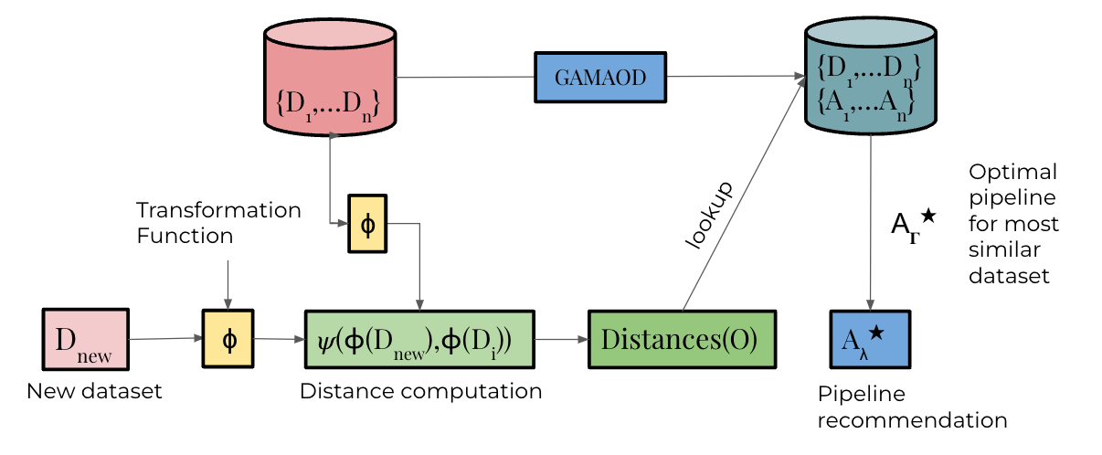
Figure 1: An overview of LOTUS

3.2.1 GAMAOD: Automated supervised learning for outlier detection

Problem Formulation: A Combined model selection and hyperparameter optimization problem  (Thornton et al., 2013) for a supervised learning task is as follows:

$$\begin{split}A^{*}_{\lambda^{*}}=\operatorname*{argmin}_{\begin{subarray}{c}\forall A^{j}\in\bm{A}\\ \forall\lambda\in\bm{\Lambda_{A}}\end{subarray}}\frac{1}{k}\sum_{f=1}^{k}L\left(A^{j}_{\lambda},\big{\{}\bm{X}^{f}_{train},\bm{y}^{f}_{train}\big{\}},\big{\{}\bm{X}^{f}_{val},\bm{y}^{f}_{val}\big{\}}\right)\end{split}$$ (5)

in equation 5, $A_{\lambda^{*}}^{*}$ is an optimal combination of learning algorithm from search space $A$ with associated hyperparameter space $\Lambda_{A}$ over $k$ cross validation folds of dataset $D$ where $D=\{X,y\}$ with training and validation splits. $L$ is our evaluation measure.

The CASH problem from equation 5 relies on the validation split to optimise for the optimal configuration. However, in unsupervised outlier detection scenario the learning algorithm does not have access to labels but the AutoML framework does. We cannot do cross validation folds in the unsupervised outlier model selection setting as the learning algorithms are trained without labels and evaluated with labels. Hence performing k-fold CV is not useful in this setting. Our modified CASH formulation to select the optimal unsupervised algorithm with access to labels is as follows:

$$\begin{split}A^{*}_{\lambda^{*}}=\operatorname*{argmin}_{\begin{subarray}{c}\forall A^{j}\in\bm{A}\\ \forall\lambda\in\bm{\Lambda_{A}}\end{subarray}}L\left(A^{j}_{\lambda},\big{\{}\bm{X}_{train}\}\big{\{}\bm{y}_{train}\big{\}}\right)\end{split}$$ (6)

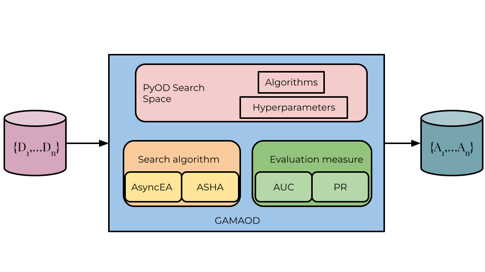
Figure 2: An overview of GAMAOD

GAMAOD: To populate our meta-data we develop an extension on top of GAMA  (Gijsbers & Vanschoren, 2021), we call this extension GAMAOD. GAMAOD’s search space consists of outlier detectors from PyOD  (Zhao et al., 2019), PyOD is a Python library for detecting outlying objects in multivariate data. GAMAOD can use different metrics to optimise for the given task like AUC score and PR.

3.2.2 LOTUS: Learning to learn with optimal transport for unsupervised scenarios

We describe LOTUS approach in algorithm 1. Our meta-learning approach has two components. First, we have a transformation function that is applied to the dataset. Let’s call this function $\phi$, which is applied on given datasets $D_{a}$ and $D_{b}$. In the second phase, we calculate the dataset similarity $\mathcal{O}$ based on some distance metric $\psi$ in equation 7. Because our distributions are lie on different metric spaces we calculate the Low Rank Gromov Wasserstein distance from equation 4 on these transformed distributions in equation 8.

$$\mathcal{O}=\psi(\phi(D_{a})\phi(D_{b}))$$ (7)

$$\mathcal{O}=\text{GW-LR}^{(r)}(\phi(D_{a})\phi(D_{b}))$$ (8)

To find the most similar dataset $\Gamma$, we take the smallest distance from datasets from our distance matrix $\{\mathcal{O}_{1},...,\mathcal{O}_{n}\}$ between a new dataset $D_{new}$ and existing datasets from $\mathcal{D}_{meta}$. which results in:

$$\Gamma=argmin\{\mathcal{O}_{1},...,\mathcal{O}_{n}\}$$ (9)

Our meta-approach for capturing the similarity metric between datasets can be described as:

$$\Gamma_{\Gamma\in\mathcal{D}_{meta}}=argmin(\text{GW-LR}^{(r)}(\phi(D_{new})\iota\{(\phi(D_{D\in\mathcal{D}_{meta}}))\}))$$ (10)

where $\iota$ is the iterator over $\mathcal{D}_{meta}$.
LOTUS then accesses the optimal pipeline from $\mathcal{A}$: $A^{*}_{\lambda^{*}new}=A^{*}_{\lambda^{*}\Gamma}$ Where $A^{*}_{\lambda^{*}new}$ is the optimal pipeline for $D_{new}$.

Algorithm 1 Pseudocode for LOTUS

Inputs: $D_{new},\mathcal{D}_{meta},\mathcal{A}$

while $D_{i}\in\mathcal{D}_{meta}$ do

     $\mathcal{O}_{i}\leftarrow\psi(\phi(D_{new},D_{i}))$ $\triangleright$ Distance calculation

$\Gamma\leftarrow\mathcal{D}_{meta}[argmin\{\mathcal{O}_{1},...,\mathcal{O}_{n}\}]$ $\triangleright$ Retrieval of most similar dataset

$A^{*}_{\lambda^{*}new}\leftarrow A^{*}_{\lambda^{*}\Gamma}$ $\triangleright$ Model Selection

4 experiments on ADBench

For our experiments, we use ADBench  (Han et al., 2022) and retrieve all tabular datasets. This collection consists of 46 datasets. As we do not have access to multiple benchmarks we use the N-1 strategy for the evaluation of our system, i.e., we take one dataset at a time from ADBench and use the other datasets in the meta-data. This ensures independent meta-training on the following datasets. We compare our approach with 7 outlier detection algorithms available in PyOD  (Zhao et al., 2019) and the current state of the art meta-learner for outlier detection MetaOD  (Zhao et al., 2021). From PyOD we compare our approach with the following algorithms: IForest  (Liu et al., 2008), ABOD  (Kriegel et al., 2008), OCSVM  (Schölkopf et al., 1999), LODA  (Pevný, 2015), KNN  (Angiulli & Pizzuti, 2002; Ramaswamy et al., 2000), HBOS  (Goldstein & Dengel, 2012).

For experimental consistency, we use the same search space for GAMAOD pretraining as MetaOD (A.3) to ensure a fair comparison. To populate our meta-data, we run GAMAOD for 2 hours on every ADBench dataset to find the optimal pipeline for a given dataset. We use an asynchronous evolutionary algorithm to iterate over the search space and return the optimal pipeline. GAMAOD uses AUC score as internal metric for model selection.

Implementation details: We use Independent Component Analysis(ICA)  (Hyvärinen & Oja, 2000) from scikit-learn  (Pedregosa et al., 2011) as our transformation function $\phi$. We use OTT-JAX library  (Cuturi et al., 2022) library to implement Low Rank Gromov Wassersstein distance. For this experiment, we set the rank parameter of Low Rank Gromov Wasserstein to 6. The model selection phase of LOTUS in our experiments is as follows: First the datasets are transformed via ICA and then converted into JAX  (Bradbury et al., 2018) pointclouds geometry objects and then we turn these distributions into a quadratic regularized optimal transport problem  (Peyré et al., 2016). We input this quadratic problem to our Gromov Wasserstein Low Rank solver which returns us the distance(cost) between two datasets. When a new dataset is given to LOTUS, the pipeline corresponding to the dataset with the lowest distance(except the new dataset itself) is chosen from the optimal pipeline database.

5 results and discussion

5.1 Experimental results

We use the Bayesian Wilcoxon signed-rank test (or ROPE test,  Benavoli et al. (2017; 2014)) to analyze the results of our experiments. ROPE defines an interval wherein the differences in model performance are considered equivalent to the null value. Using this test allows us to compare model performances in a more practical sense. We set the ROPE value to 1% for our experiments. We use the baycomp library  (Benavoli et al., 2017) to run and visualize the analyses.

LOTUS vs MetaOD: The ROPE test on AUC scores comparing LOTUS and MetaOD are shown in Figure 3. There is a 74.2 % probability that LOTUS is better than MetaOD. LOTUS proves to be more robust than MetaOD, since $p(LOTUS)>p(MetaOD)$. We show the per-dataset performances in Appendix A.1.

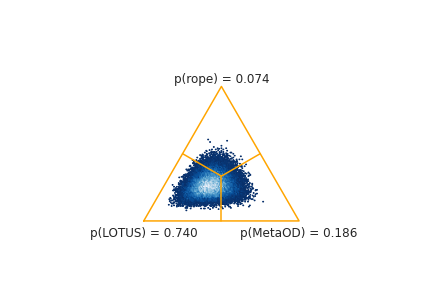
Figure 3: ROPE test LOTUS vs MetaOD.

Results against other estimators: ROPE testing on the results of ROCAUC performance of LOTUS vs other estimators are shown in Table 1. LOTUS proves to be significantly better than other techniques, with default parameters, in PyOD. In this case $P(LOTUS)>>P(PyOD_{estimators})$, Figure 5 shows the simplex plots of MetaOD vs other estimators. We also include a Critical Difference Plot of performances between LOTUS and PyOD estimators (lower is better) in Figure 4. The detailed experimental results are reported in appendix A.1 table 3.

Figure 4: Comparison of average rank (lower is better) of methods w.r.t. performance across datasets in ADBench.

Estimator name	p(LOTUS)	p(rope)	p(Estimator)
IForest	0.99954	0.0	0.00046
ABOD	1.0	0.0	0.0
OCSVM	1.0	0.0	0.0
LODA	1.0	0.0	0.0
KNN	1.0	0.0	0.0
HBOS	0.99982	0.0	0.00018
COF	1.0	0.0	0.0

Table 1: Rope testing results with LOTUS vs PyOD estimators with rope=1%

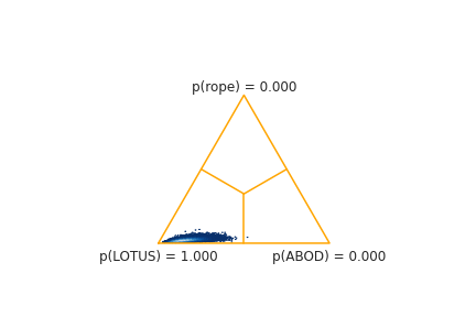
(a) LOTUS vs ABOD

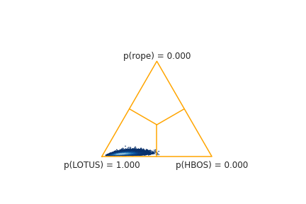
(b) LOTUS vs HBOS

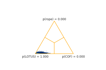
(c) LOTUS vs COF

(d) LOTUS vs IForest

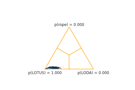
(e) LOTUS vs LODA

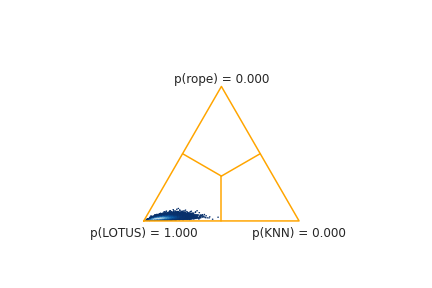
(f) LOTUS vs KNN

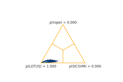
(g) LOTUS vs OCSVM

Figure 5: ROPE test result of LOTUS vs (a) ABOD (b) HBOS (c) COF (d) IForest (e) LODA (f) KNN (g) OCSVM

5.2 Using optimal transport distances as a similarity measure

In our experiments, we show that LOTUS is more robust and better than current state of the art meta-learner MetaOD for unsupervised outlier detection tasks and other outlier detection algorithms in default configuration.

In our method we experimentally show that using optimal transport distances like GW-LR is a feasible approach for dataset similarity and meta-learning. We would like to emphasize that this similarity measure should only be used as a relative similarity measure, for e.g. in our case where we use this similarity measure to find the most similar dataset from a collection of datasets in $\mathcal{D}_{meta}$. To estimate to what degree datasets are similar Nies et al. (2021) proposes optimal transport based correlation measures that can be leveraged. Our approach assumes that Wasserstein distances can capture intrinsic properties of datasets and can capture the similarity between them, Alvarez-Melis & Fusi (2020) also proposes their approach with optimal transport distances to provide some sort of distance between dataset.

5.3 Related Works

In this section we will discuss the difference between closest approaches to LOTUS which are MetaOD and MetaBu.

5.3.1 LOTUS vs MetaOD

LOTUS and MetaOD solve the same problem of model selection problem for unsupervised outlier detection. The major difference in LOTUS and MetaOD is meta-feature generation. LOTUS aims to capture the similarity of the given source and target representations via optimal transport. MetaOD captures similarity with a combination of landmark-features and model-based features and uses a rank-based criteria called discounted cumulative gain for model selection. MetaOD also uses stochastic algorithms such as Isolation Forest and LODA for model-based meta-feature generation which means that the absolute dataset similarity and ranking can differ based on the number of runs. LOTUS on the other hand uses non stochastic methods for distance calculation. Our approach is generalises more than MetaOD as well for different unsupervised tasks as it aims to find similar dataset independent of task, whereas MetaOD’s similarity is highly coupled with the task of outlier detection.

5.3.2 LOTUS vs MetaBu

MetaBu  (Rakotoarison et al., 2022) was proposed as a solution to cold start problem in supervised learning scenario. Rakotoarison et al. (2022) uses Fused-Gromov-Wasserstein distance with multi dimensional scaling  (Cox & Cox, 2008) by first extracting meta-features from the target representation and source representation and proximal gradient method  (Xu et al., 2020). LOTUS on the other hand uses independent component analysis and Low Rank Gromov Wasserstein. LOTUS is much faster than MetaBu simply because of computational complexity differences between Low Rank Gromov Wasserstein($O(n)$) and Fused Gromov Wasserstein($O(n^{3})$). LOTUS is a simpler approach as well as compared to MetaBu(2 phases vs 5 phases). Lastly, LOTUS is a solution for unsupervised setting whereas MetaBu relies on landmark features from PyMFE  (Alcobaça et al., 2020) which are more reliable for datasets with labels. Similar to MetaOD, MetaBu setting is limited to only one task (supervised classification) as it relies on landmark-features which require labels. LOTUS therefore can generalize to more tasks than MetaBu.

5.4 limitations

1. LOTUS: LOTUS depends on the quality of meta-data, i.e. range of datasets and algorithms in our case. In the worst case scenario, if there are no similar datasets in the $\mathcal{D}_{meta}$, LOTUS can recommend a dataset which is not sufficiently similar to new dataset. On the other hand, it is expected to improve as more benchmarks and datasets with different properties become available.

2. OT distance: The computation cost of GW-LR on really large datasets can still be very high. In these cases we recommend using stratified sampling or random sampling depending on the nature of dataset and problem.

3. Parameter tuning: Tuning rank of GW-LR can be tricky. Low rank can result in faster computation but high loss and high rank can result in less efficient algorithm. Scetbon et al. (2022) states an experiment where they study the affect of rank of GW-LR. This rank can also be tuned by minimizing the loss between GW and GW-LR.

6 conclusion and future work

Model selection for unsupervised outlier detection is a challenging task. We do not have efficient internal metrics for evaluating an algorithm without ground truth. In this work, we proposed a new meta-learner: LOTUS, which uses optimal transport distances to capture the similarity between datasets and uses that similarity measure to recommend pipelines from a meta-data. To run these experiments, we also developed another tool GAMAOD which is an extension of GAMA and allows users to find optimal outlier detection algorithms in a supervised setting. Through our experiments, we demonstrate that LOTUS outperforms MetaOD and other built-in estimators in PyOD. The LOTUS approach also enables researchers to use a simplified meta-learning framework as compared to other landmark and model-based meta-features methods where meta-features are highly specialized according to the domain.

We believe that our approach can be easily extended as a meta-learner to perform model selection in other unsupervised machine learning tasks as well. These include clustering, distance metric learning, density estimation and covariance estimation. This approach can also be used as a meta-learner to warm-start neural architecture search(NAS) problems.

7 reproducibilty statement

We opensource both LOTUS and GAMAOD with hyperparameters used for this experiment. We also provide scripts which can be used to perform these experiment for just one dataset without making the meta-data first(not reccomended). We aim to provide modularity to researchers therefore we users them to save and retrieve meta-data in whatever format they want. More information about reproducing our experiments can be found in the README.md of the supplementary code repository. To reproduce LOTUS for other tasks and dataset, users are simply required to change the datasets and algorithms in meta-data. The approach works out of the box for other scenarios. While reproducing the experiments, the results can differ due to stochasticity of few algorithms.

Appendix A Appendix

A.1 Performances

Table 2 contains the performances of LOTUS and MetaOD on 42 datasets, We had to eliminate 4 datasets from this experiment because MetaOD returned invalid models for these datasets(i.e. models with invalid values). Scores are in bold where AUC of LOTUS $>$ MetaOD or differ by less than a %. The dataset names are as they were in ADBench  (Han et al., 2022).

Dataset	LOTUS	MetaOD
19_landsat	0.7902	0.5931
25_musk	0.9895	0.9655
24_mnist	1.0000	1.0000
32_shuttle	0.9216	0.9163
23_mammography	0.6434	0.6477
42_WBC	0.8521	0.8655
15_Hepatitis	0.9353	0.9353
43_WDBC	0.8548	0.9671
12_fault	0.9246	0.9043
10_cover	0.9463	0.9436
34_smtp	0.2744	0.5212
11_donors	0.8064	0.8049
29_Pima	0.8804	0.7197
37_Stamps	0.9275	0.9339
44_Wilt	0.7765	0.5327
40_vowels	0.8491	0.9355
8_celeba	0.9908	0.9906
1_ALOI	0.8954	0.8957
30_satellite	0.8913	0.7890
26_optdigits	0.9996	0.9997
2_annthyroid	0.8472	0.8445
41_Waveform	0.9758	0.9413
28_pendigits	0.8597	0.9265
4_breastw	0.7466	0.7438
21_Lymphography	0.9441	0.9861
20_letter	0.9701	0.9891
39_vertebral	0.7634	0.8424
47_yeast	0.9089	0.9097
3_backdoor	1.0000	1.0000
13_fraud	0.9646	0.8904
45_wine	0.9841	0.9481
22_magic.gamma	0.9322	0.8122
9_census	0.9819	1.0000
7_Cardiotocography	0.9392	0.9378
35_SpamBase	0.9446	0.9015
46_WPBC	0.7811	0.8088
36_speech	1.0000	0.4344
6_cardio	0.9794	0.9793
31_satimage-2	0.9552	0.8100
18_Ionosphere	0.8072	0.8338
27_PageBlocks	0.7164	0.7668
5_campaign	0.9922	0.9996

Table 2: AUC scores of MetaOD vs LOTUS on ADBench

Table 3 reports the auc scores over datasets from ADBench. The bold number shows scores where LOTUS is better than all other estimators in PyOD.

Dataset	IForest	ABOD	OCSVM	LODA	KNN	HBOS	COF	LOTUS
44_Wilt	0.471963	0.568222	0.301310	0.408280	0.472095	0.281412	0.544269	0.7765
6_cardio	0.943738	0.498576	0.939676	0.892753	0.741544	0.865343	0.544550	0.9794
43_WDBC	0.987241	0.987241	0.989655	0.987586	0.960345	0.998966	0.771034	0.8548
4_breastw	0.976321	0.976321	0.778694	0.981964	0.947386	0.969329	0.381366	0.7466
42_WBC	0.993567	0.993567	0.994103	0.995980	0.911954	0.991691	0.754757	0.8521
47_yeast	0.431011	0.417114	0.448353	0.492504	0.413668	0.410032	0.428639	0.9089
45_wine	0.735205	0.735205	0.681612	0.923158	0.471241	0.891757	0.412289	0.9841
5_campaign	0.692549	0.642977	0.645556	0.566477	0.696817	0.771387	0.564588	0.9922
46_WPBC	0.522489	0.522489	0.475911	0.562133	0.419170	0.555259	0.495170	0.7811
7_Cardiotocography	0.752439	0.539423	0.810433	0.785916	0.582569	0.623355	0.572511	0.9392
8_celeba	0.757810	0.757810	0.761861	0.718291	0.632204	0.805965	0.393545	0.9908
9_census	0.598140	0.598140	0.523211	0.325589	0.650628	0.633393	0.413254	0.9819
39_vertebral	0.377788	0.377788	0.427308	0.284423	0.417163	0.282356	0.321923	0.7634
41_Waveform	0.669757	0.698172	0.474443	0.611266	0.782120	0.639714	0.804121	0.9758
38_thyroid	0.979620	0.979620	0.867786	0.699534	0.951152	0.952834	0.871991	0.7910
40_vowels	0.708373	0.956714	0.532701	0.655924	0.971722	0.646130	0.849763	0.8491
3_backdoor	0.734361	0.734361	0.802264	0.708914	0.738679	0.665487	0.728995	1.0000
32_shuttle	0.996250	0.618768	0.987461	0.951075	0.678578	0.994925	0.557606	0.9216
31_satimage-2	0.996844	0.762625	0.983527	0.987126	0.909884	0.985936	0.451384	0.9552
26_optdigits	0.771433	0.525541	0.527237	0.623480	0.398194	0.852822	0.423611	0.9996
1_ALOI	0.501898	0.609567	0.532848	0.549594	0.555634	0.478001	0.635583	0.8954
35_SpamBase	0.657074	0.390792	0.520510	0.273952	0.515358	0.651507	0.416468	0.9446
36_speech	0.469975	0.729473	0.462061	0.448529	0.473192	0.476358	0.553156	1.0000
34_smtp	0.696899	0.670223	0.018006	0.372124	0.744582	0.878626	0.890630	0.2744
22_magic.gamma	0.704407	0.799144	0.594241	0.635940	0.823228	0.681717	0.663549	0.9322
23_mammography	0.859409	0.859409	0.854704	0.814810	0.859614	0.871755	0.792004	0.6434
24_mnist	0.794443	0.750330	0.834765	0.743575	0.828259	0.619057	0.733384	1.0000
20_letter	0.581556	0.880889	0.485185	0.627407	0.867111	0.540593	0.829704	0.9701
30_satellite	0.707795	0.538013	0.605468	0.609243	0.646056	0.768130	0.556999	0.8913
19_landsat	0.495534	0.500057	0.374050	0.382382	0.577134	0.556768	0.542057	0.7902
37_Stamps	0.909527	0.909527	0.878255	0.944582	0.746473	0.928582	0.636364	0.9275
18_Ionosphere	0.867847	0.867847	0.765359	0.858325	0.862297	0.667416	0.850478	0.8072
21_Lymphography	0.997003	0.997003	0.993506	0.667582	0.512862	0.995005	0.934316	0.9441
25_musk	0.999923	0.085936	0.818675	0.959047	0.701124	1.000000	0.400387	0.9895
17_InternetAds	0.700473	0.673305	0.710028	0.580881	0.712320	0.704318	0.693902	1.0000
16_http	1.000000	1.000000	0.995308	0.000000	0.001340	0.994638	0.583110	0.7106
15_Hepatitis	0.742736	0.742736	0.722262	0.772817	0.467871	0.813292	0.425388	0.9353
14_glass	0.818496	0.818496	0.459264	0.632274	0.740799	0.791758	0.882668	0.8374
13_fraud	0.934023	0.941569	0.914391	0.751185	0.916394	0.941169	0.914591	0.9646
11_donors	0.794215	0.794215	0.723436	0.260784	0.829936	0.763981	0.720262	0.8064
12_fault	0.571477	0.676490	0.494426	0.436072	0.713079	0.479224	0.612146	0.9246
2_annthyroid	0.824922	0.824922	0.606069	0.305845	0.730291	0.691522	0.704828	0.8472
27_PageBlocks	0.889696	0.684494	0.892650	0.753280	0.769997	0.788657	0.673234	0.7164
28_pendigits	0.949714	0.673023	0.938642	0.951140	0.705836	0.921169	0.475639	0.8597
29_Pima	0.660016	0.660016	0.580166	0.606169	0.685681	0.713573	0.566752	0.8804
10_cover	0.914310	0.767605	0.886407	0.866889	0.899776	0.795243	0.870260	0.9463

Table 3: AUC Scores: LOTUS vs PyOD estimators with default configuration

A.2 Baslines

The 8 baslines estimators and frameworks are listed below with brief description from PyOD’s  (Zhao et al., 2019) documentation for reference here:

1. MetaOD: MetaOD is the first automated tool for outlier detection. MetaOD use collaborative filtering, landmark and model based meta-features to recommend the model for given task.

2. IForest: IsolationForest ‘isolates’ observations by randomly selecting a feature and then randomly selecting a split value between the maximum and minimum values of the selected feature.

3. LOF:The anomaly score of each sample is called Local Outlier Factor. It measures the local deviation of density of a given sample with respect to its neighbors. It is local in that the anomaly score depends on how isolated the object is with respect to the surrounding neighborhood. More precisely, locality is given by k-nearest neighbors, whose distance is used to estimate the local density. By comparing the local density of a sample to the local densities of its neighbors, one can identify samples that have a substantially lower density than their neighbors. These are considered outliers.

4. ABOD:For an observation, the variance of its weighted cosine scores to all neighbors could be viewed as the outlying score.

5. HBOS: Histogram- based outlier detection assumes the feature independence and calculates the degree of outlier by building histograms.

6. KNN: kNN class for outlier detection. For an observation, its distance to its kth nearest neighbor could be viewed as the outlying score.

7. COF: Connectivity-Based Outlier Factor uses the ratio of average chaining distance of data point and the average of average chaining distance of k nearest neighbor of the data point, as the outlier score for observations.

8. LDOA: Lightweight on-line detector of anomalies detects anomalies in a dataset by computing the likelihood of data points using an ensemble of one-dimensional histograms.

9. OCSVM: One class support vector machines unsupervised outlier Detection. Estimate the support of a high-dimensional distribution.

A.3 LOTUS+GAMAOD search space and MetaOD reproducibility

We implement the same searchspace as MetaOD github repository for a fair comparison. , MetaOD also uses all the existing datasets from ADbench. We believe that we have fairly evaluated MetaOD against out baseline. We believe that our Benchmark setting was more challenging than the one evaluated in Zhao et al. (2021) where it take child and parent datasets.

References

- Achille et al. (2021) Alessandro Achille, Giovanni Paolini, Glen Mbeng, and Stefano Soatto. The information complexity of learning tasks, their structure and their distance. Information and Inference: A Journal of the IMA, 10(1):51–72, 01 2021. ISSN 2049-8772. doi: 10.1093/imaiai/iaaa033. URL https://doi.org/10.1093/imaiai/iaaa033.
- Aggarwal (2013) Charu C. Aggarwal. Outlier analysis. In Springer New York, 2013.
- Alcobaça et al. (2020) Edesio Alcobaça, Felipe Siqueira, Adriano Rivolli, Luís P. F. Garcia, Jefferson T. Oliva, and André C. P. L. F. de Carvalho. Mfe: Towards reproducible meta-feature extraction. Journal of Machine Learning Research, 21(111):1–5, 2020. URL http://jmlr.org/papers/v21/19-348.html.
- Alvarez-Melis & Fusi (2020) David Alvarez-Melis and Nicoló Fusi. Geometric dataset distances via optimal transport. ArXiv, abs/2002.02923, 2020.
- Angiulli & Pizzuti (2002) Fabrizio Angiulli and Clara Pizzuti. Fast outlier detection in high dimensional spaces. In PKDD, 2002.
- Benavoli et al. (2014) Alessio Benavoli, Giorgio Corani, Francesca Mangili, Marco Zaffalon, and Fabrizio Ruggeri. A bayesian wilcoxon signed-rank test based on the dirichlet process. In Eric P. Xing and Tony Jebara (eds.), Proceedings of the 31st International Conference on Machine Learning, volume 32 of Proceedings of Machine Learning Research, pp. 1026–1034, Bejing, China, 22–24 Jun 2014. PMLR. URL https://proceedings.mlr.press/v32/benavoli14.html.
- Benavoli et al. (2017) Alessio Benavoli, Giorgio Corani, Janez Demšar, and Marco Zaffalon. Time for a change: a tutorial for comparing multiple classifiers through bayesian analysis. Journal of Machine Learning Research, 18(77):1–36, 2017. URL http://jmlr.org/papers/v18/16-305.html.
- Bradbury et al. (2018) James Bradbury, Roy Frostig, Peter Hawkins, Matthew James Johnson, Chris Leary, Dougal Maclaurin, George Necula, Adam Paszke, Jake VanderPlas, Skye Wanderman-Milne, and Qiao Zhang. JAX: composable transformations of Python+NumPy programs, 2018. URL http://github.com/google/jax.
- Campos et al. (2015) Guilherme Oliveira Campos, Arthur Zimek, Jörg Sander, Ricardo J. G. B. Campello, Barbora Micenková, Erich Schubert, Ira Assent, and Michael E. Houle. On the evaluation of unsupervised outlier detection: measures, datasets, and an empirical study. Data Mining and Knowledge Discovery, 30:891–927, 2015.
- Castiello et al. (2005) Ciro Castiello, Giovanna Castellano, and Anna Maria Fanelli. Meta-data: Characterization of input features for meta-learning. In Vicenç Torra, Yasuo Narukawa, and Sadaaki Miyamoto (eds.), Modeling Decisions for Artificial Intelligence, pp. 457–468, Berlin, Heidelberg, 2005. Springer Berlin Heidelberg. ISBN 978-3-540-31883-5.
- Cho & Eo (2016) HyungJun Cho and Soo-Heang Eo. Outlier detection for mass spectrometric data. Methods in molecular biology, 1362:91–102, 2016.
- Chow & keung Tse (1990) Shein-Chung Chow and Siu keung Tse. Outlier detection in bioavailability/bioequivalence studies. Statistics in medicine, 9 5:549–58, 1990.
- Cox & Cox (2008) Michael A. A. Cox and Trevor F. Cox. Multidimensional Scaling, pp. 315–347. Springer Berlin Heidelberg, Berlin, Heidelberg, 2008. ISBN 978-3-540-33037-0. doi: 10.1007/978-3-540-33037-0˙14. URL https://doi.org/10.1007/978-3-540-33037-0_14.
- Cuturi (2013) Marco Cuturi. Sinkhorn distances: Lightspeed computation of optimal transport. In NIPS, 2013.
- Cuturi et al. (2022) Marco Cuturi, Laetitia Meng-Papaxanthos, Yingtao Tian, Charlotte Bunne, Geoff Davis, and Olivier Teboul. Optimal transport tools (ott): A jax toolbox for all things wasserstein. ArXiv, abs/2201.12324, 2022.
- Egan & Morgan (1998) William J. Egan and Stephen L. Morgan. Outlier detection in multivariate analytical chemical data. Analytical chemistry, 70 11:2372–9, 1998.
- Feurer et al. (2015) Matthias Feurer, Aaron Klein, Katharina Eggensperger, Jost Springenberg, Manuel Blum, and Frank Hutter. Efficient and robust automated machine learning. In C. Cortes, N. Lawrence, D. Lee, M. Sugiyama, and R. Garnett (eds.), Advances in Neural Information Processing Systems, volume 28. Curran Associates, Inc., 2015. URL https://proceedings.neurips.cc/paper/2015/file/11d0e6287202fced83f79975ec59a3a6-Paper.pdf.
- Feurer et al. (2020) Matthias Feurer, Katharina Eggensperger, Stefan Falkner, Marius Lindauer, and Frank Hutter. Auto-sklearn 2.0: Hands-free automl via meta-learning. arXiv:2007.04074 [cs.LG], 2020.
- Gao & Chaudhari (2021) Yansong Gao and Pratik Chaudhari. An information-geometric distance on the space of tasks. In Marina Meila and Tong Zhang (eds.), Proceedings of the 38th International Conference on Machine Learning, volume 139 of Proceedings of Machine Learning Research, pp. 3553–3563. PMLR, 18–24 Jul 2021. URL https://proceedings.mlr.press/v139/gao21a.html.
- Gijsbers & Vanschoren (2021) Pieter Gijsbers and Joaquin Vanschoren. Gama: A general automated machine learning assistant. In Yuxiao Dong, Georgiana Ifrim, Dunja Mladenić, Craig Saunders, and Sofie Van Hoecke (eds.), Machine Learning and Knowledge Discovery in Databases. Applied Data Science and Demo Track, pp. 560–564, Cham, 2021. Springer International Publishing. ISBN 978-3-030-67670-4.
- Goix (2016) Nicolas Goix. How to evaluate the quality of unsupervised anomaly detection algorithms?, 2016. URL https://arxiv.org/abs/1607.01152.
- Goldstein & Dengel (2012) Markus Goldstein and Andreas R. Dengel. Histogram-based outlier score (hbos): A fast unsupervised anomaly detection algorithm. 2012.
- Han et al. (2022) Songqiao Han, Xiyang Hu, Hailiang Huang, Minqi Jiang, and Yue Zhao. ADBench: Anomaly detection benchmark. In Thirty-sixth Conference on Neural Information Processing Systems Datasets and Benchmarks Track, 2022. URL https://openreview.net/forum?id=foA_SFQ9zo0.
- Hutter et al. (2019) Frank Hutter, Lars Kotthoff, and Joaquin Vanschoren. Automated machine learning: Methods, systems, challenges. Automated Machine Learning, 2019.
- Hyvärinen & Oja (2000) Aapo Hyvärinen and Erkki Oja. Independent component analysis: algorithms and applications. Neural networks : the official journal of the International Neural Network Society, 13 4-5:411–30, 2000.
- Kriegel et al. (2008) Hans-Peter Kriegel, Matthias Schubert, and Arthur Zimek. Angle-based outlier detection in high-dimensional data. In Proceedings of the 14th ACM SIGKDD International Conference on Knowledge Discovery and Data Mining, pp. 444–452, 2008. ISBN 9781605581934. doi: 10.1145/1401890.1401946.
- Li et al. (2020) Yuening Li, Daochen Zha, Na Zou, and Xia Hu. Pyodds: An end-to-end outlier detection system with automated machine learning. Companion Proceedings of the Web Conference 2020, 2020.
- Liu et al. (2008) Fei Tony Liu, Kai Ming Ting, and Zhi-Hua Zhou. Isolation forest. 2008 Eighth IEEE International Conference on Data Mining, pp. 413–422, 2008.
- Ma et al. (2021a) Martin Q. Ma, Yue Zhao, Xiaorong Zhang, and Leman Akoglu. A large-scale study on unsupervised outlier model selection: Do internal strategies suffice? CoRR, abs/2104.01422, 2021a. URL https://arxiv.org/abs/2104.01422.
- Ma et al. (2021b) Zhiwei Ma, Daniel S. Reich, Sarah Dembling, Jeff H. Duyn, and Alan P. Koretsky. Outlier detection in multimodal mri identifies rare individual phenotypes among 20,000 brains. bioRxiv, 2021b.
- Marques et al. (2015) Henrique O. Marques, Ricardo J. G. B. Campello, Arthur Zimek, and Jorg Sander. On the internal evaluation of unsupervised outlier detection. In Proceedings of the 27th International Conference on Scientific and Statistical Database Management, SSDBM ’15, New York, NY, USA, 2015. Association for Computing Machinery. ISBN 9781450337090. doi: 10.1145/2791347.2791352. URL https://doi.org/10.1145/2791347.2791352.
- Nies et al. (2021) Thomas Giacomo Nies, Thomas Staudt, and Axel Munk. Transport dependency: Optimal transport based dependency measures. 2021.
- Pedregosa et al. (2011) F. Pedregosa, G. Varoquaux, A. Gramfort, V. Michel, B. Thirion, O. Grisel, M. Blondel, P. Prettenhofer, R. Weiss, V. Dubourg, J. Vanderplas, A. Passos, D. Cournapeau, M. Brucher, M. Perrot, and E. Duchesnay. Scikit-learn: Machine learning in Python. Journal of Machine Learning Research, 12:2825–2830, 2011.
- Pevný (2015) Tomás Pevný. Loda: Lightweight on-line detector of anomalies. Machine Learning, 102:275–304, 2015.
- Peyré & Cuturi (2019) Gabriel Peyré and Marco Cuturi. Computational optimal transport. Found. Trends Mach. Learn., 11:355–607, 2019.
- Peyré et al. (2016) Gabriel Peyré, Marco Cuturi, and Justin Solomon. Gromov-wasserstein averaging of kernel and distance matrices. In Maria Florina Balcan and Kilian Q. Weinberger (eds.), Proceedings of The 33rd International Conference on Machine Learning, volume 48 of Proceedings of Machine Learning Research, pp. 2664–2672, New York, New York, USA, 20–22 Jun 2016. PMLR. URL https://proceedings.mlr.press/v48/peyre16.html.
- Rakotoarison et al. (2022) Herilalaina Rakotoarison, Louisot Milijaona, Andry RASOANAIVO, Michele Sebag, and Marc Schoenauer. Learning meta-features for autoML. In International Conference on Learning Representations, 2022. URL https://openreview.net/forum?id=DTkEfj0Ygb8.
- Ramaswamy et al. (2000) Sridhar Ramaswamy, Rajeev Rastogi, and Kyuseok Shim. Efficient algorithms for mining outliers from large data sets. SIGMOD Rec., 29(2):427–438, may 2000. ISSN 0163-5808. doi: 10.1145/335191.335437. URL https://doi.org/10.1145/335191.335437.
- Scetbon & Cuturi (2022) Meyer Scetbon and Marco Cuturi. Low-rank optimal transport: Approximation, statistics and debiasing. NeurIPS 2022, abs/2205.12365, 2022.
- Scetbon et al. (2021) Meyer Scetbon, Marco Cuturi, and Gabriel Peyré. Low-rank sinkhorn factorization. In Marina Meila and Tong Zhang (eds.), Proceedings of the 38th International Conference on Machine Learning, volume 139 of Proceedings of Machine Learning Research, pp. 9344–9354. PMLR, 18–24 Jul 2021. URL https://proceedings.mlr.press/v139/scetbon21a.html.
- Scetbon et al. (2022) Meyer Scetbon, Gabriel Peyré, and Marco Cuturi. Linear-time gromov Wasserstein distances using low rank couplings and costs. In Kamalika Chaudhuri, Stefanie Jegelka, Le Song, Csaba Szepesvari, Gang Niu, and Sivan Sabato (eds.), Proceedings of the 39th International Conference on Machine Learning, volume 162 of Proceedings of Machine Learning Research, pp. 19347–19365. PMLR, 17–23 Jul 2022. URL https://proceedings.mlr.press/v162/scetbon22b.html.
- Schölkopf et al. (1999) Bernhard Schölkopf, Robert C. Williamson, Alex Smola, John Shawe-Taylor, and John C. Platt. Support vector method for novelty detection. In NIPS, 1999.
- Stern et al. (2010) David Stern, Ralf Herbrich, Thore Graepel, Horst Samulowitz, Luca Pulina, and Armando Tacchella. Collaborative expert portfolio management. In Proceedings of the Twenty-Fourth AAAI Conference on Artificial Intelligence AAAI-10 (to appear), July 2010. URL https://www.microsoft.com/en-us/research/publication/collaborative-expert-portfolio-management/.
- Thornton et al. (2013) Chris Thornton, Frank Hutter, Holger H. Hoos, and Kevin Leyton-Brown. Auto-WEKA: Combined selection and hyperparameter optimization of classification algorithms. In 19th ACM SIGKDD International Conference on Knowledge Discovery and Data Mining, pp. 847–855, 2013. ISBN 9781450321747. doi: 10.1145/2487575.2487629.
- Vanschoren (2018) Joaquin Vanschoren. Meta-learning: A survey. ArXiv, abs/1810.03548, 2018.
- Vanschoren (2019) Joaquin Vanschoren. Meta-learning. Hutter et al. (2019), pp. 39–68.
- Villani (2008) Cédric Villani. Optimal transport: Old and new. 2008.
- Xu et al. (2020) Hongteng Xu, Dixin Luo, Ricardo Henao, Svati Shah, and Lawrence Carin. Learning autoencoders with relational regularization. In Hal Daumé III and Aarti Singh (eds.), Proceedings of the 37th International Conference on Machine Learning, volume 119 of Proceedings of Machine Learning Research, pp. 10576–10586. PMLR, 13–18 Jul 2020. URL https://proceedings.mlr.press/v119/xu20e.html.
- Zhao et al. (2019) Yue Zhao, Zain Nasrullah, and Zheng Li. Pyod: A python toolbox for scalable outlier detection. J. Mach. Learn. Res., 20:96:1–96:7, 2019.
- Zhao et al. (2021) Yue Zhao, Ryan Rossi, and Leman Akoglu. Automatic unsupervised outlier model selection. In M. Ranzato, A. Beygelzimer, Y. Dauphin, P.S. Liang, and J. Wortman Vaughan (eds.), Advances in Neural Information Processing Systems, volume 34, pp. 4489–4502. Curran Associates, Inc., 2021. URL https://proceedings.neurips.cc/paper/2021/file/23c894276a2c5a16470e6a31f4618d73-Paper.pdf.