One-body dynamical correlation function of Lieb-Liniger model at finite temperature

Abstract

The dynamical correlated properties of one-dimensional (1D) Bose gases provide profound understanding of novel physics emergent from collective excitations, for instance the breakdown of off-diagonal long-range order, and the establishment of Tomonaga-Luttinger liquid (TLL) theory. However, due to the non-perturbative nature of 1D many-body systems, the exact evaluation of correlation functions is notoriously difficult. Here by means of form factor approach based on algebraic Bethe ansatz and numerics, we present a thorough study on the one-body dynamical correlation function (1BDCF) of the Lieb-Liniger model at finite temperature. The influence of thermal fluctuation and dynamical interaction on the behavior of 1BDCF has been demonstrated and analyzed from various perspectives, including the spectral distribution, the line-shape of 1BDCF, and the static correlations etc. The static correlation properties, i.e. the momentum distribution and one body density matrix are shown in good agreement with the TLL prediction.

In the last two decades, a growing interest in low-dimensional quantum many-body systems has stimulated tremendous success in both theoretical and experimental developments of quantum physics [1, 3, 4, 5, 2]. In contrast to Landau’s quasi-particles emergent from condensed matter problems of higher dimensions [6, 7], the bosonic collective excitations [8, 9] take over the main role of low-energy physics for the one-dimensional (1D) strongly correlated systems. Consequently, significantly different phenomena away from the quasi-particle picture occur at low temperature in 1D, such as the absence of true Bose-Einstein condensate (BEC) in homogenous Bose gases [10], fractional spin and holon excitations [11], spin-charge separation [12, 13, 14], breakdown of thermalization in 1D quantum gases [15, 16, 17], etc. The key to understanding such unique physics lies in the correlation functions of either zero or finite temperatures, yet the non-perturbative nature brings with a big challenge on their exact evaluation [9]. In this letter, making use of quantum itegrable theory, we thoroughly study the finite temperature one-body dynamical correlation function (1BDCF) of the Lieb-Liniger model with an arbitrary interaction.

The Lieb-Liniger model describes $N$ spinless bosons confined in a length $L$ via contact interaction [18], and its Hamiltonian reads

$$H=-\sum_{i=1}^{N}\frac{\partial^{2}}{\partial x_{i}^{2}}+2c\sum_{i>j}^{N}\delta\left(x_{i}-x_{j}\right),$$ (1)

where $c>0$ ($c<0$) specifies the interaction strength of repulsion (attraction) and hereafter we only consider the repulsive interaction. The physics of this model is governed by two dimensionless parameters simultaneously, i.e. interaction strength $\gamma=c/n$ and temperature $\tau=T/T_{d}$. Here we denoted the particle density $n=N/L$ and degenerate temperature $T_{d}=\hbar^{2}n^{2}/(2mk_{B})$, respectively. By tuning these parameters the system would vary across several different regimes, quasi-condensate, Tonks-Girardeau (TG) gas, degenerate regime, decoherence regime and quantum criticality etc [19, 20]. In the TG limit $\gamma\rightarrow\infty$, the one-particle density matrix was derived at zero and finite temperatures by the trick of Bose-Fermi map [21, 22, 23], and in the presence of trap potential as well [26, 27, 28, 24, 25]. Away from this limit, on basis of pseudopotential hamiltonian and a combination of generalized Hartree-Fock approximation and random phase approximation, the dynamic structure factor (DSF) in strongly correlated region was obtained up to a correction of $1/\gamma$ order [29]. While with the application of Hellmann-Feynman theorem, the pair correlation function was calculated [30, 19], and a general expression for higher order static correlation function in strongly correlated regime was found through the asymptotic Bethe ansatz solution [31, 32]. Besides, the edge singularity of dynamical correlation functions was predicted by the nonlinear Tomonaga-Luttinger liquid (TLL) theory [33, 3].

Being the simplest quantum integrable system [18], the Lieb-Liniger model has been acting as a major subject of textbook materials for quantum many-body physics [9, 34, 35]. Nevertheless, the study of correlation functions is still notoriously difficult due to complexity of many-body eigenstates [35]. Towards this end, much effort has been devoted to finding the determinant representations of various correlators through the algebraic Bethe ansatz (ABA) technique [36, 37, 38, 39]. These formidable formulas prevent the full access to correlated properties until their combination with numerics come true [40, 41, 43, 42, 44, 45, 46], making form factor approach manifests itself as an answer to the appeal of cutting-edge cold atom experiments [47]. On the other hand, by restricting the number of excitations the DSF and spectral function were obtained for the low density region by utilizing the thermodynamic form factor [48]. The quantum integral technique enables the evaluation of non-universal prefactors present in the bosonization theory as well [49].

Here we present a through study of 1BDCF for the Lieb-Liniger model at zero and finite temperatures with arbitrary interaction strengths, by utilizing form factor approach on basis of ABA and numerics. The spectral distributions, the line-shape of 1BDCF, the momentum distribution, and the one-body density matrix are obtained to reveal a deep insight into the dynamical behaviour of the Lie-Liniger model at finite temperatures.

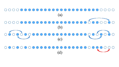
Figure 1: Illustration of quantum numbers: (a) depicts the distribution of QNs for the ground state, an analogy of Fermi sea. For a $N$-particle system, the ground state QNs range consecutively from $-(N-1)/2$ to $(N-1)/2$. (b) shows the QNs of one-pair of particle-hole (p-h) excitation. (c) demonstrates how a thermodynamic eigenstate is achieved by means of multi-pairs of p-h excitation, where the distribution of QNs is obviously symmetric. (d). shows an example of relative ‘excitation’ over the original thermal equilibrium eigenstate, giving birth to states responsible for the secondary peak in Fig. 3.

By virtue of periodical boundary conditions and Bethe wave function, the diagonalization of Hamiltonian in Eq. 1 is equivalent to solving a set of transcendental equations, i.e. Bethe ansatz equations (BAEs) [18]

$$\lambda_{j}+\frac{1}{L}\sum_{k=1}^{N}\theta\left(\lambda_{j}-\lambda_{k}\right)=\frac{2\pi}{L}I_{j},\quad j=1,\dots,N$$ (2)

where $\theta(x)=2\arctan(x/c)$, $\lambda_{j}$ and $I_{j}$ are the pseudomomentum and corresponding quantum number (QN) respectively. A set of $\{I_{j}\}$ uniquely determines a quantum state (represented by a set of $\{\lambda_{j}\}$), vice versa. Those QNs take integer (half-integer) if $N$ is odd (even). The total momentum and energy of the system are expressed in terms of pseudomomenta, $P_{\{\lambda\}}=\sum_{j=1}^{N}\lambda_{j}$ and $E_{\{\lambda\}}=\sum_{j=1}^{N}\lambda_{j}^{2}$. It is convenient to illustrate the eigenstates of system by making use of the distribution for QNs. The ground state is depicted by a Fermi sea-like distribution, over which pairs of particle-hole (p-h) excitations simply generate excited states, see Fig. 1 (a) and (b). This distribution in thermodynamic limit becomes a continuous function of pseudomomentum.

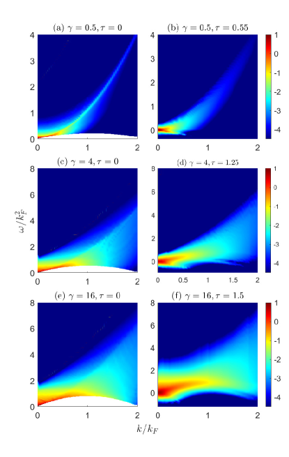
Figure 2: The logarithmic 1BDCF at $k$ - $\omega$ plane with different temperature $\tau$ and interaction $\gamma$ of system size $N=L=60$. The momentum and energy are measured in units of Fermi momentum and Fermi energy respectively. The left panel is for zero temperature and the right for finite temperature. The sum rules of (a)-(f) are respectively 99.99 %, 99.83 %, 99.63 %, 97.63 %, 98.90 % and 98.99 %.

The 1BDCF of our interest is defined by

$$g_{1}(k,\omega)=\int_{0}^{L}\textmd{d}x\int_{-\infty}^{\infty}\textmd{d}t\,e^{\textmd{i}(\omega t-kx)}\langle\Psi^{\dagger}(x,t)\Psi(0,0)\rangle_{T}$$ (3)

where $\Psi(x,t)$ ($\Psi^{\dagger}(x,t)$) is the bosonic field operator of annihilation (creation) and $\langle\cdots\rangle_{T}$ stands for a statistical expectation value at finite temperature $T$. The standard way for evaluation of this ensemble average needs computation of the partition function, which however is extremely hard to compute for a strongly correlated system. It turns out this difficulty can be circumvented by means of quantum integrability. The saddle point state is well described by the thermodynamic Bethe ansatz equation (TBA) [35, 50], which can be solved once particle density and temperature is specified. Utilizing the TBA, we determine the distribution of the QNs, and thus the problem of ensemble expectation can be simplified, similar to the situation for the ground state. After inserting a completeness relation of intermediate states, the 1BDCF is further given by

$$g_{1}\left(k,\omega\right)=2\pi L\sum_{\{\mu\}}\frac{\|\langle\{\mu\}|\Psi(0,0)|\{\lambda\}_{T}\rangle\|^{2}}{\|\{\lambda\}_{T}\|^{2}\|\{\mu\}\|^{2}}\,\delta_{k,P_{\mu,\lambda}}\delta\left(\omega-E_{\mu,\lambda}\right),$$ (4)

where $|\{\lambda\}_{T}\rangle$ is the thermal equilibrium eigenstate. In the above equation, we denoted $O_{\mu,\lambda}\equiv O_{\{\mu\}}-O_{\{\lambda\}}$ with $O=P$ and $E$. $\delta_{m,n}$ and $\delta(x)$ are the Kronecker- and Dirac-delta functions, respectively. $\langle\{\mu\}|\Psi(0,0)|\{\lambda\}_{T}\rangle$ is called form factor and $\|\{\nu\}\|^{2}$ is the norm square of eigenstate, both of which can be numerically calculated through the determinants with entries represented by pseudomomenta [41].

In principle, the sum is taken over the whole Hilbert space, which is however impossible in practice. We therefore incorporate the states with significant contributions to the correlation function as many as possible until a satisfying precision [44]. This navigation of states of course can be fulfilled by generating 1-, 2- , …, and $m$-pairs of p-h excitations over the ground state. Nevertheless, in the situation of finite temperature, this will be a waste of computation resource. Instead, we define a ‘relative’ excitation over the thermodynamic equilibrium state as is shown in Fig. 1 (d), and then count states by manipulating such type of ‘relative’ excitations. This thought comes from a naive observation that the most relevant states should be of similar looking i.e. distribution of QNs. A simple example of how the algorithm works can be found in Supplementary Materials. The saturation is readily checked by following sum rule [41]

$$\sum_{k}n(k)=\frac{N}{L},$$ (5)

where $n(k)=\int_{-\infty}^{\infty}\frac{\textmd{d}\omega}{2\pi L}g_{1}(k,\omega)$ is exactly the momentum distribution.

In the strongly degenerate regime ($\tau\ll 1$), it is reasonable to judge 1BDCF to be similar to its zero temperature situation, merely differing with a temperature-dependent perturbation. In a weakly interacting regime ($\tau\ll\gamma\ll 1$ or $\gamma\ll\tau\ll\sqrt{\gamma}$), the Gross-Pitaevskii equation provides a way to understand the quantum correlation functions. Away from this limit, increasing temperature gradually destroys the phase coherence and thus system eventually arrives at the decoherent regime. Here we focus on the regime $\tau\sim\sqrt{\gamma}$, where the competition between thermal fluctuation and interaction recomposes the correlated properties.

The frequency-momentum resolved 1BDCF is demonstrated in Fig. 2, and without losing generality the particle density is set by $n=1$. The left panel shows that at zero temperature, the spectral weight mostly concentrates on the Lieb-II dispersion relation, and spreads continuously to the Lieb-I dispersion relation, where the former (latter) dispersion corresponds to adding a particle (hole) outside (inside) of the Fermi sea [51]. In the right panel of finite temperature case, immediate differences are observed with the non-vanishing spectral distribution in the half-plane of negative energy. This is easy to understand from the perspective of p-h excitation as being given in Fig. 1. In Fig. 1 (c), the thermal equilibrium eigenstate means a melted Fermi sea, and thus there exists such a type of relative ‘excitation’ that the particles jump inward over the indicated thermal state. A typical example of such an ‘excitation’ is depicted by the red arrow in Fig. 1 (d), which generates the states bearing non-vanishing spectral contribution while possessing lower energy than the original thermal equilibrium eigenstate. In quantum degenerate regime, the thermal equilibrium egienstate contains very few holes lying almost on the Fermi points, which leaves no further room for above inward ‘excitations’. This in consequence suppresses the spectral distribution in negative energy plane. On the other hand, at either zero or finite temperatures. The spectral distribution in the continuum between upper and lower thresholds implies the breakdown of quasi-particle picture with a replacement of collective excitations, manifesting the special role of interaction in 1D.

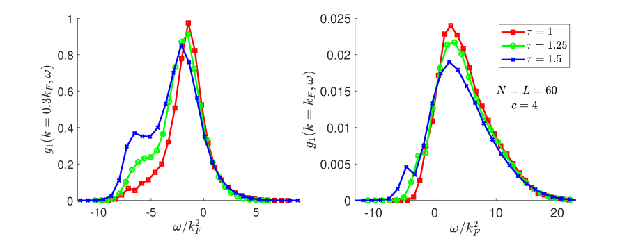
Figure 3: (a) and (b) show the line shape of $g_{1}(k,\omega)$ vs $\omega$ with $k=0.3k_{F}$ and $k=k_{F}$ respectively. The system size is $N=L=60$, and dimensionless interaction is $\gamma=4$. The energy is measured in unit of Fermi energy. The red, green, and blue lines stand for the rescaled temperatures $\tau=1.0,1.25$ and $1.5$ respectively.

In Fig. 3, the line shape of 1BDCF with a given momentum is calculated by taking the case of intermediate interaction strength $\gamma=4$. At zero temperature, there is an analog of Fermi edge singularity lying on the lower spectral threshold [33, 44, 41], which is smeared here by the thermal fluctuation. Moreover, the thermal fluctuation manifests itself by amplifying the relative contribution from the states generated by multi-pairs of p-h excitations, and redistributing the spectral weight along the energy axis, in accordance with Fig. 2. Along with an increase of the temperature, a hump emerges in the plane of negative energy gradually. Like what is discussed before, this emergent peak arises from the states produced by the jump-inward ’excitations’ relative to the original thermal equilibrium state. Besides, the main peak is lowered in this process, whose loss of spectral weight is compensated by this little hump.

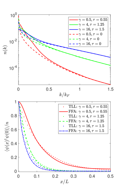
Figure 4: (a). The momentum distributions at different temperature $\tau$ and interaction strength $\gamma$. All data comes from Fig. 2. For the sake of a clear visibility, we take logarithmic momentums. The dotted and solid lines stand for zero and finite temperatures, respectively. (b). The one-body density matrix with different temperature $\tau$ and interaction strength $\gamma$. The solid and dotted lines respectively correspond to the TLL predictions and our results derived from form factor approach (FFA). The parameters of $(\gamma,\tau)$ for red, green and blue lines are $(0.5,0.55),(4,1.25),$ and $(16,1.5)$.

The static correlation function of 1BDCF (i.e. the momentum distribution) is obtained by integrating out the frequency, whose Fourier transformation is the one-body density matrix. In Fig. 4 (a) we compare the momentum distribution at zero and finite temperatures on basis of data from Fig. 2. Despite of no true BEC in the Lieb-Liniger model, the weak interaction still results in a prominent zero-momentum occupation than the larger interactions do. A direct comparison shows obvious discrepancies between the lines of zero and finite temperatures. This is simply a result of disturbance from the thermal fluctuation on particles of small momentum. This is evidenced by observing the height of humps in Fig. 3 (a) and (b) as well. Meanwhile, owing to interaction effect, the weaker is the interaction the larger is the discrepancy. The one-body density matrix is shown in Fig. 4 (b), where the comparison of our results and the TLL prediction [52] is seen in a good agreement. We observe that the validity of TLL theory requires the linearization of low-lying excited spectrum which works well if $k\ll 1$.

Last but not least, we discuss the finite-size effect. Since a general estimation is hard to make, we only can calculate and compare the 1BDCF at a fixed momentum for different system sizes. It is shown in Fig. 5 that the curves of $N=L=60$ and $N=L=80$ agree well with each other, with slight difference from that of $N=L=40$. Hence it is safe to conduct our calculation for a system of $N=L=60$.

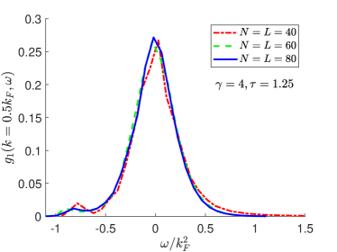
Figure 5: 1BDCF vs $\omega$ at $k=0.5k_{F}$ of different system sizes. The dimensionless interaction strength and rescaled temperature are set as $\gamma=4$ and $\tau=1.25$, respectively. The solid blue, dashed green and dotted red lines denote the cases of $N=L=80,60$ and $40$, respectively.

In conclusion, a detailed study on the finite temperature 1BDCF of the Lieb-Liniger model with arbitrary interaction strengths has been presented by using the form factor approach and numerics. In particular, we have considered the regime far away from the GP and Tonks-Girardeau limit. By comparing situations of zero and finite temperatures, the results of spectral distribution, line-shape of 1BDCF, momentum distribution and one-body density matrix have explicitly shown the competition between thermal fluctuation and dynamical interaction. For the one-particle density matrix, a good agreement between our result and the prediction from the TLL theory is observed. We have discussed the spectral distribution in the half-plane of negative energy which can be regarded as the relative ‘excitation’ over thermal equilibrium eigenstate, leading to the little hump therein. Our research sheds light on quantum many-body dynamical correlation driven by thermal and dynamical interaction, and provides a straightforward application in 1D integrable quantum gases with the cutting-edge cold-atom experiment.

Acknowledgments. SC and YYC contributed equally. SC thanks the hospitality of Institute of Modern Physics in Northwest University where part of this work was completed. This work is supported by National Natural Science Foundation of China Grants Nos. 12088101, 12104372, 12047511, 12047502, 12134015, 11874393 and 12121004. SC and HQL acknowledge the computational resources from the Beijing Computational Science Research Center.

Note Added. After the appearance of this work on arXiv: 2211.00282, recently another paper [45] arXiv: 2301.09224 has come up with improvements on ABACUS [43], and posed the difficulty in evaluating 1BDCF at finite temperatures, which have been overcome by our algorithm presented here and in [44].

References

- [1] M. A. Cazalilla, R. Citro, T. Giamarchi, E. Orignac, and M. Rigol, Rev. Mod. Phys. 83, 1405 (2011).
- [2] M. A. Cazalilla, J. Phys. B. 37, S1 (2004).
- [3] A. Imambekov, T. L. Schmidt and L. I. Glazman, Rev. Mod. Phys. 84, 1253 (2012).
- [4] X.-W. Guan, M. T. Batchelor, and C.-H. Lee, Rev. Mod. Phys. 85, 1633 (2013).
- [5] X.-W. Guan and P. He, Rep. Prog. Phys. 85, 114001 (2022).
- [6] L. D. Landau, JETP 3, 920 (1957).
- [7] P. W. Anderson, Basic Notions of Condensed Matter Physics (Benjamin Cummings, Penlo Park, 1984).
- [8] F. D. M. Haldane, Phys. Rev. Lett. 47, 1840 (1981); J. Phys. C 14, 2585 (1981).
- [9] T. Giamarchi, Quantum Physics in One Dimension (Oxford University Press, Oxford, 2004).
- [10] S. Giorgini, L. P. Pitaevskii and S. Stringari, Rev. Mod. Phys. 80, 1215 (2008).
- [11] F. H. L. Essler, H. Frahm, F. Göhmann, A. Klümper and V. E. Korepin, The One-Dimensional Hubbard Model (Cambridge University Press, Cambridge, 2005).
- [12] T. A. Hilker, G. Salomon, F. Grusdt, A. Omran, M. Boll, E. Demler, I. Bloch, C. Gross, Science 357, 484 (2017).
- [13] J. Vijayan, P. Sompet, G. Salomon, J. Koepsell, S. Hirthe, A. Bohrdt, F. Grusdt, I. Bloch, and C. Gross, Science 367, 186 (2020).
- [14] R. Senaratne, D. Cavazos-Cavazos, S. Wang, F. He, Y.-T. Chang, A. Kafle, H. Pu, X.-W. Guan, and R. G. Hulet, Science 376, 1305 (2022).
- [15] T. Kinoshita, T. Wenger, and D. S. Weiss, Nature 440, 900 (2006).
- [16] T. Langen, S. Erne, R. Geiger, B. Rauer, T. Schweigler, M. Kuhnert, W. Rohringer, I. E. Mazets, T. Gasenzer, and J. Schmiedmayer, Science 348, 207 (2015).
- [17] J. M. Wilson, N. Malvania, Y. Le, Y. Zhang, M. Rigol, D. S. Weiss, Science 367, 1461 (2020).
- [18] E. H. Lieb, and W. Liniger, Phys. Rev. 130, 1605 (1963); E. H. Lieb, ibid. 130, 1616 (1963).
- [19] K. V. Kheruntsyan, D. M. Gangardt, P. D. Drummond, and G. V. Shlyapnikov, Phys. Rev. Lett. 91, 040403 (2003); Phys. Rev. A 71, 053615 (2005).
- [20] X.-W. Guan and M. T. Batchelor, J. Phy. A 44, 102001 (2011).
- [21] M. Girardeau, J. Math. Phys. 1, 516 (1960); Phys. Rev. 139, B500 (1965).
- [22] A. Lenard, J. Math. Phys. 5, 930 (1964); ibid. 7, 1268 (1966).
- [23] H. G. Vaidya, and C. A. Tracy, Phys. Rev. Lett. 42, 3 (1979); J. Math. Phys. 20, 2291 (1979).
- [24] R. Pezer and H. Buljan, Phys. Rev. Lett. 98, 240403 (2007).
- [25] J. Settino, N. Lo Gullo, F. Plastina, and A. Minguzzi, Phys. Rev. Lett. 126, 065301 (2021).
- [26] A. Colcelli, J. Viti, G. Mussardo, and A. Trombettoni, Phys. Rev. A 98, 063633 (2018).
- [27] A. Colcelli, G. Mussardo, and A. Trombettoni, Euro. Phys. Lett. 122, 50006 (2018).
- [28] A. Colcelli, N. Defenu, G. Mussardo, and A. Trombettoni, Phys. Rev. B 102, 184510 (2020).
- [29] J. Brand, and A. Yu. Cherny, Phys. Rev. A 72, 033619 (2005); A. Yu. Cherny and J. Brand, ibid. 73, 023612 (2006).
- [30] D. M. Gangardt and G. V. Shlyapnikov, Phys. Rev. Lett. 90, 010401 (2003).
- [31] D. M. Gangardt and G. V. Shlyapnikov, New. J. Phys. 5, 79 (2003).
- [32] E. J. K. P. Nandani , R. A. Römer, S.-N. Tan, and X.-W. Guan, New. J. Phys. 18, 055014 (2016).
- [33] A. Imambekov, and L. I. Glazman, Phys. Rev. Lett. 100, 206805 (2008); ibid. 102, 126405 (2009).
- [34] F. Franchini, An Introduction to Integrable Techniques for One-Dimensional Quantum Systems (Springer, Cham, 2017)
- [35] V. E. Korepin, N. M. Bogoliubov, and A. G. Izergin, Quantum Inverse Scattering Method and Correlation Functions (Cambridge University Press, Cambridge, 1993).
- [36] V. E. Korepin, Commun. Math. Phys. 86, 391 (1982).
- [37] V. E. Korepin, Commun. Math. Phys. 94, 93 (1984).
- [38] N. A. Slavnov, Teor. Mat. Fiz. 79, 232 (1989); ibid. 82, 389 (1990).
- [39] T. Kojima, V. E. Korepin, and N. A. Slavnov, Commun. Math. Phys. 188, 657 (1997); ibid. 189, 709 (1997).
- [40] J.-S. Caux, and P. Calabrese, Phys. Rev. A 74, 031605(R) (2006).
- [41] J.-S. Caux, P. Calabrese, and N. A. Slavnov, J. Stat. Mech. (2007) P01008.
- [42] M. Panfil, and J.-S. Caux, Phys. Rev. A 89, 033605 (2014).
- [43] J.-S. Caux, J. Math. Phys. 50, 095214 (2009).
- [44] S. Cheng, Y.-Y. Chen, X.-W. Guan, W.-L. Yang, R. Mondaini, and H.-Q. Lin, arXiv:2209.15221v1.
- [45] A. J. J. M. de Klerk, and J.-S. Caux, arXiv: 2301.09224.
- [46] Y.-Y. Chen, S. Cheng and X.-W. Guan, in preparation.
- [47] N. Fabbri, D. Clément, L. Fallani, C. Fort and M. Inguscio, Phys. Rev. A 83, 031604(R) (2011); B. Yang, Y.-Y. Chen, Y.-G. Zheng, H. Sun, H.-N. Dai, X.-W. Guan, Z.-S. Yuan, and J.-W. Pan, Phys. Rev. Lett. 119, 165701 (2017).
- [48] E. Granet and F. H. L. Essler, SciPost. Phys. 9, 082 (2020); E. Granet, J. Phys. A. 54, 154001 (2021).
- [49] A. Shashi, L. I. Glazman, J.-S. Caux, and A. Imambekov, Phys. Rev. B 84, 045408 (2011); A. Shashi, M. Panfil, J.-S. Caux, and A. Imambekov, Phys. Rev. B 85, 155136 (2012).
- [50] C. N. Yang and C. P. Yang, J. Math. Phys. 10, 1115 (1969).
- [51] See Eq. (I.4.29) of Ref. [35] for more explanation.
-
[52]
The TLL prediction comes from following formula cf. Ref. [2],
where is the Luttinger parameter, and is the phase correlation length.