ActGraph: Prioritization of Test Cases Based on Deep Neural Network Activation Graph

Abstract

Widespread applications of deep neural networks (DNNs) benefit from DNN testing to guarantee their quality. In the DNN testing, numerous test cases are fed into the model to explore potential vulnerabilities, but they require expensive manual cost to check the label. Therefore, test case prioritization is proposed to solve the problem of labeling cost, e.g., activation-based and mutation-based prioritization methods. However, most of them suffer from limited scenarios (i.e. high confidence adversarial or false positive cases) and high time complexity. To address these challenges, we propose the concept of the activation graph from the perspective of the spatial relationship of neurons. We observe that the activation graph of cases that triggers the model’s misbehavior significantly differs from that of normal cases. Motivated by it, we design a test case prioritization method based on the activation graph, ActGraph, by extracting the high-order node features of the activation graph for prioritization. ActGraph explains the difference between the test cases to solve the problem of scenario limitation. Without mutation operations, ActGraph is easy to implement, leading to lower time complexity. Extensive experiments on three datasets and four models demonstrate that ActGraph has the following key characteristics. (i) Effectiveness and generalizability: ActGraph shows competitive performance in all of the natural, adversarial and mixed scenarios, especially in RAUC-100 improvement ($\sim\times$1.40). (ii) Efficiency: ActGraph does not use complex mutation operations and runs in less time ($\sim\times$1/50) than the state-of-the-art method.

1 INTRODUCTION

Deep neural networks (DNNs) are widely applied in object recognition [1], image classification [2], natural language processing [3], autonomous vehicles [4], etc. But it is still threatened by uncertain inputs. For example, a car in autopilot mode recognized a white truck as a cloud in the sky and caused a serious traffic accident [5]. Therefore, it is crucial to test the DNN to find vulnerabilities before deployment.

In the testing phase, numerous diverse test cases are fed into the DNN in order to evaluate the reliability of the model. These test cases require expensive manual labeling and verification. To reduce the cost of labeling, a feasible solution is to prioritize test cases to find more vulnerabilities. These test cases are more likely to expose DNN vulnerabilities are marked in advance, improving the efficiency of DNN testing.

Some test case prioritization methods have been proposed to address the labeling cost problem. They can be divided into three categories, including Neuron Coverage (NC)-based [6, 7, 8, 9, 10], model activation-based [11, 12, 13, 14] and mutation-based [15] test case prioritization methods. NC-based methods draw on the concept of test coverage [16, 17, 18] from the traditional software testing to measure the adequacy of test cases. But some studies [19, 20, 21] have pointed out that it isn’t strongly correlated between NC and misclassified inputs, so NC cannot be effectively applied to prioritization.

Model activation-based prioritization methods can be divided into confidence-based and embedding-based test case prioritization methods. Confidence-based methods [11, 12] extract the probability distribution of test cases in the DNN confidence layer. They believe that the correctly classified cases should output higher probabilities, but misclassified cases should output multiple similar probabilities. This assumption limits their application scenarios. For example, Carlini-Wagner (C&W) [22] adversarial cases can cause the DNN to output high confidence in the wrong class, so the effect of confidence-based methods will be significantly reduced. On the other hand, embedding-based prioritization methods [13, 14] generally extract the hidden layer outputs of test cases. They prioritize test cases with inconsistencies based on the differences between adversarial and normal cases. However, they cannot effectively prioritize false positive (FP) cases, because the confusion of hidden layer features directly leads to the misclassification of the model.

Mutation-based test case prioritization, i.e., PRioritizing test inputs via Intelligent Mutation Analysis (PRIMA), is the state-of-the-art (SOTA) method, which uses mutation operations to make test cases as different as possible to produce different prediction results, arguing that it is easier to reveal the DNN vulnerabilities. The time complexity of PRIMA is $O\left(nm_{1}+nm_{2}N_{\theta}\right)$, where $n$ is the total number of test cases, $m_{1}$ is the number of sample mutations, $m_{2}$ is the number of model mutations and $N_{\theta}$ is the number of parameters in the model mutation. Since $m_{1}$, $m_{2}$ and $N_{\theta}$ are usually very large, PRIMA has to take higher time complexity than activation-based methods ($O(n\log{n})$).

Based on the above analysis, the existing test case prioritization methods show limitations in two aspects: (i) Limited Scenarios. Model activation-based prioritization methods have limited application scenarios. Specifically, confidence-based prioritization methods consider that misclassified cases have multiple similar probabilities, thus they are less effective for adversarial cases with high confidence. On the other hand, embedding-based prioritization methods are less effective for FP cases, due to that the embedding features of FP cases are confused with the wrong classes. (ii) High Complexity. Mutation-based prioritization has a high time complexity since most of them require numerous mutations, memory read and write, and mutation query operations. Therefore, its time complexity is higher than activation-based methods.

Therefore, to address the prioritization challenges, we explore the in-depth relationship between the test cases and the model’s dynamic features. Although the existing model activation-based prioritization methods have extracted features in the hidden layer or the confidence layer, but they overlook some more fine-grained features, such as the neuron’s activation. Therefore, we propose graph-level neuron activation features for test cases, to extract the activation graph between DNN layers. The activation graph is defined as the connection relationship of neurons. We study the differences in the activation graph for test cases. An illustration is carried out shown in Fig. 1. The activation graphs for the normal, FP, and C&W adversarial test cases are shown. It is a LeNet-5 [23] trained on MNIST [23]. Fig. 1 (a) and (b) are normal test cases with class labels 9 and 7, respectively. Fig. 1 (c) and (d) are misclassified as 9, which are FP and adversarial cases, respectively. We only show weighted edge values greater than 0.4, in order to show the activation graph clearly. The size of the node is determined by its node feature value. We observe the distribution differences in activation graphs for the test cases. Specifically, the edges of the last layer of the activation graph of the normal cases are only connected to the correct node, as shown in Fig. 1 (a) and (b). On the contrary, the misclassified cases will connect not only the correct node but also the wrong node in the last layer of the activation graph, as shown in Fig. 1 (c) and (d). Comparing the activation graph of normal case (Fig. 1 (b)) and adversarial case (Fig. 1 (d)), we observe that the similar distribution of edges in shallow layers (L1, L2), but the differences distribution of edges gradually increase in deeper layers (L3, L4 and L5).

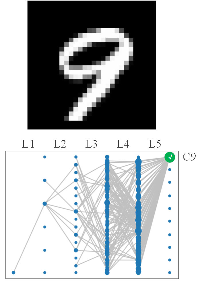
(a) Normal case “9”

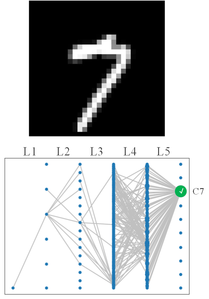
(b) Normal case “7”

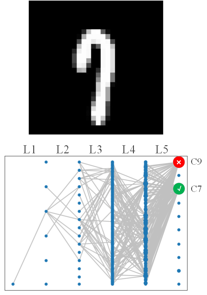
(c) FP case “9”

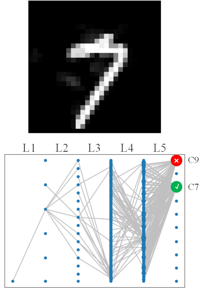
(d) Adversarial case “9”

Figure 1: The activation graphs of three type cases. (a) Activation graph of the normal digital 9. (b) Activation graph of the normal digital 7. (c) Activation graph of the false positive digital 7, but misclassified as 9. (d) Activation graph of the C&W digital 7, but misclassified as 9.

Therefore, we propose a model activation graph-based test case prioritization, namely ActGraph. ActGraph regards the neurons of DNN as nodes, and the adjacency matrix as the connection relationship between nodes. Then, the node features and the adjacency matrix are aggregated by message passing [24], the aggregated node features will contain the features of neighbor nodes and the structural information between nodes, which can be effectively used for test case prioritization. ActGraph has the following two key characteristics.

(i) Effectiveness and generalizability. ActGraph extracts the finer-grained activation features of the test cases on the model, and converts the model activations into the spatial relationship of neurons, which can solve the limitation problem of the scene based on the model activation method. ActGraph can prioritize multiple types of test cases by learning one type of cases, which is more general than model activation-based methods.

(ii) Efficiency. ActGraph uses the graph to extract high-level node features instead of mutation operations, which is much more efficient than the mutation-based approaches.

In addition, ActGraph builds a ranking model using Learning-to-Rank (L2R) [25], which can effectively prioritize test cases by learning the node features of test cases. According to the priority results of the ActGraph, the test cases that trigger the vulnerability can be marked earlier, thereby greatly improving the efficiency of DNN testing and effectively saving development time.

The main contributions are summarized as follows.

• By identifying the limitations of existing prioritization methods, we propose the activation graph, and find that cases that trigger model vulnerabilities and normal cases in the activation graph.

• Motivated by the observation, we propose a novel test case prioritization method, namely ActGraph. It extracts the spatial relationship between neuron nodes, calculates the center node feature in the activation graph, and adopts L2R model to intelligently combine center node feature to achieve efficient test case prioritization.

• Comprehensive experiments have been conducted on three datasets and four models to verify the effectiveness and efficiency of ActGraph. It outperforms the SOTA baselines in both natural and adversarial scenarios, especially in RAUC-100 ($\sim\times$1.40).

The remainder of this paper is organized as follows. We describe the related work in Section 2. In Section 3, we describe the designed ActGraph method in detail. Experimental results are provided in Section 4. Threats to validity are described in Section 5 and conclusions are made in Section 6.

2 RELATED WORKS

2.1 Test Case Prioritization for DNNs

Some DNN test case prioritization methods are proposed to solve the labeling-cost problem. According to the different dynamic features of DNNs for test cases, they can be categorized into: NC-based [6, 7, 8, 9, 10], model activation-based [11, 12, 13, 14] and mutation-based [15] test case prioritization methods.

NC-based test case prioritization. NC borrows the concept of test coverage from traditional software testing to measure the adequacy of test cases, which was first proposed by Pei et al. [6]. They argue that DNNs with higher coverage are more secure and reliable when the input is uncertain. Based on this, Guo et al. [7] continuously mutate the input slightly, with maximizing the NC and the predicted difference between the original and the mutated input to guide the generation of test cases. But some studies [19, 20, 21] have pointed out that NC and misclassified inputs do not have a strong correlation, so cannot be effectively applied to test case prioritization.

Model activation-based test case prioritization. Test case prioritization methods based on model activation can be divided into confidence-based and embedding feature-based. Confidence-based prioritization methods generally obtain the confidence output of the DNN. From a statistical point of view, they assume that correctly classified test cases should have high probability, and misclassified or abnormal test cases have multiple similar probabilities. For example, Feng et al. [11] proposed DeepGini based on the Gini impurity, which can quickly identify test samples that may lead to DNN misclassification. Shen et al. [12] proposed Multiple-Boundary Clustering and Prioritization (MCP) to uniformly select high-priority test cases from all boundary regions by dividing test cases into multiple boundary regions. Embedding feature-based prioritization methods believe that the deep layer of the DNN can better represent the high-level features of the input cases, so the last layer of hidden layer features of the DNN output is generally obtained. Kim et al. [13] proposed Surprise Adequacy (SA) to measure the adequacy of test cases for DNN testing by calculating the difference in hidden layer features between test cases and training data, including Likelihood-based Surprise Adequacy (LSA) and Distance-based Surprise Adequacy (DSA). LSA refers to estimating the density of the embedding features of the test cases on the training data, while DSA defines the Euclidean distance between the embedding features of the test cases and the training data. They show that DSA is more suitable for classification models.

Mutation-based test case prioritization. Wang et al. [15] proposed PRIMA, which prioritizes those test cases that produce different prediction results through fuzzy mutation operations (including input mutation and model mutation), arguing that this is more likely to reveal DNN vulnerabilities.

In addition, some test case sampling methods are proposed to improve the efficiency of DNN testing [26, 27, 28, 29, 30], to estimate the accuracy of DNN by sampling a few test cases. Our work aims to identify more bug-revealing test cases earlier by prioritizing test cases.

2.2 Graph Structure of DNNs

Several studies have constructed DNNs as Graphs (DAG) to explore the performance of DNNs, such as interpretability, generalization and performance analysis. Naitzat et al. [31] demonstrated the superiority of ReLu activation by studying the variation of the Betty number of two classes of DNN. Filan [32] et al. proposed to directly represent the fully connected layer as a weighted undirected graph, where each neuron corresponds to a node. Rieck [33] et al. proposed neural persistence, a measure of the topological complexity of network structures that can give a criterion for early stopping of training. They proposed ”Unroll”, and converting convolutional layers into graphs. Then, Vahedian et al. [34] proposed a “Rolled” graph representation of convolutional layers to solve the DNN performance prediction problem by capturing the early DNN dynamics during the training phase. To maintain the semantic meaning of the convolutional layers, they represent each filter as a node and link the filters in successive layers by weighted edges. Zhao et al. [35] proposed feature entropy to quantitatively identify individual neuron states of a specific class.

In general, most of the existing DAG studies focus on the relationship between the structural parameters of the DNN and the overall behavior of the DNN. ActGraph and the existing DAG mainly have the following differences: i) The methods of constructing the graph are different. The graph of ActGraph uses the DNN structure and multi-layer activation, unlike past works that only consider the DNN structure; ii) The application scenarios are different. ActGraph is used for test case prioritization in DNN testing.

3 APPROACH

3.1 Overview

Existing DAG studies have been able to convert the DNN into the graph, discussing the dynamic properties of the DNN model [32, 33, 34, 35]. They used an undirected weighted graph to treat neurons as nodes and the weights of the model as weighted edges between nodes. But they did not consider expressing the activation information of case to graph. Different from them, we use a directed weighted graph to take the model weights as the skeleton of the graph, and map the activation values to the graph, so that the feature of the test case is expressed on the graph. For convenience, the definitions of symbols used in this paper are listed in Table 1.

Table 1: The definitions of symbols.

Symbol	Definition
$x$	a test case
$n_{i}^{l}$	the $i$-th neuron of the $l$-th layer
$F_{i}^{l}$	the feature map of $n_{i}^{l}$
$\varphi_{i}^{l}$	the average and normalized value of $F_{i}^{l}$
$\theta$	the model weights of the trained DNN
$W$	the average and normalized weights of $\theta$
$D=(V,E)$	the direct weighted graph with sets of nodes and edges
$v_{i}$	the $i$-th node of $D$
$\left\langle v_{j},v_{i}\right\rangle$	the directed edge from $v_{j}$ to $v_{i}$
$\Gamma_{D}^{-}(v_{i})$	the set of predecessors of $v_{i}$
$A$	the adjacency matrix of $D$
$nf$	the node feature
$cnf$	the center node feature
$AGG(\cdot)$	the aggregation function of the message passing
$y$	the flag of whether the $x$ triggers the model vulnerability (0 or 1)
$\Omega(\cdot)$	the regularization function
$T$	the number of trees of xgboost

We propose a novel test case prioritization method based on model activation graph, namely ActGraph. It consists of three stages. i) Test Case Activation: the test cases are fed into the trained DNN, and each layer of the DNN outputs activation values (Section 3.2); ii) Feature Extraction: activation graphs are constructed based on the activations of DNN’s each layer, and the adjacency matrix and node features are extracted on the activation graphs. Finally the center node features are obtained by message passing aggregation (Section 3.3); iii) Ranking Model Building: ActGraph adopts the framework of L2R to build a ranking model, which can utilize the center node features, for prioritizing test cases (Section 3.4). The framework of ActGraph is shown in Fig. 2.

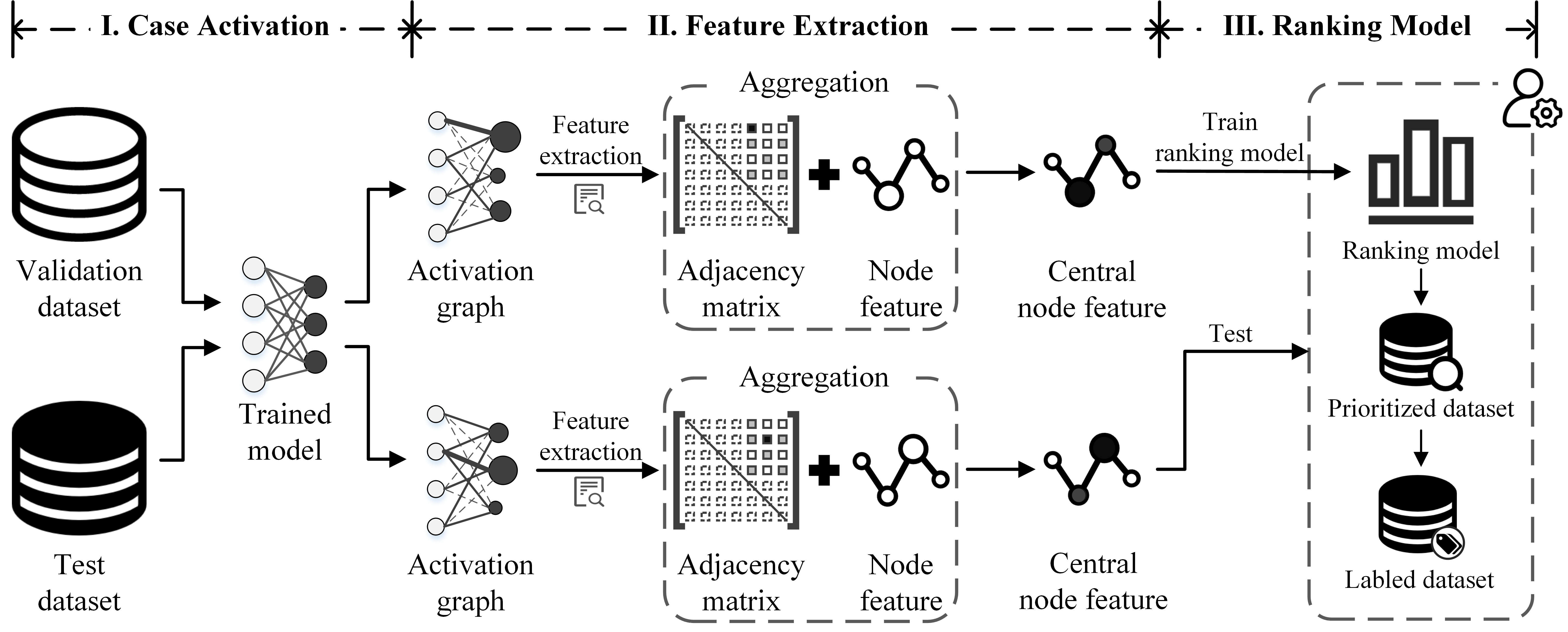
Figure 2: The framework of ActGraph, which be divided into three stages: test case activation, the feature of activation graph extraction and ranking model building.

3.2 Test Case Activation

ActGraph is a model activation-based test case prioritization method that runs during the test phase. Test cases are input to the DNN, and each layer outputs activation values. In order to facilitate the construction of the graph, the weights and activations of each neuron are averaged, and the weights and activations of each layer are normalized.

For a trained DNN and a test case $x$. DNN has $L$ layers, $n_{i}^{l}$ is the $i$-th neuron of the $l$-th layer. The case $x$ is input to the DNN, and get the output of each layer of neurons in the DNN. The activation value $\varphi_{i}^{l}$ of $n_{i}^{l}$ is calculated as:

$$\centering\varphi_{i}^{l}(x)=\frac{1}{Height_{l}\times Width_{l}}\sum_{Height_{l}}\sum_{Width_{l}}F_{i}^{l}(x)\@add@centering$$ (1)

where $F_{i}^{l}(x)\in\mathbb{R}^{Height_{l}\times Width_{l}\times Channel_{l}}$ is the feature map of $n_{i}^{l}$ output when $x$ is input. For the convolutional layer, the output dimension is $Height_{l}\times Width_{l}$, and the dimension of the fully connected layer is $1\times 1$.

The neuron activation value $\varphi^{l}(x)$ of each layer performs the max-min normalization, which normalizes $\varphi^{l}(x)$ to the [0,1] range, is calculated as:

$$\centering\varphi^{l}(x)=\frac{\varphi^{l}(x)-min(\varphi^{l}(x))}{max(\varphi^{l}(x))-min(\varphi^{l}(x))}\@add@centering$$ (2)

For the neuron $n_{i}^{l}$, its neuron weight is calculated as:

$$\centering w_{j,i}^{l-1,l}=\frac{1}{Height_{l}^{\theta}\times Width_{l}^{\theta}}\sum_{Height_{l}^{\theta}}\sum_{Width_{l}^{\theta}}\theta_{j,i}^{l-1,l}\@add@centering$$ (3)

where $\theta_{j,i}^{l-1,l}\in\mathbb{R}^{Height_{l}^{\theta}\times Width_{l}^{\theta}}$ represents the weight parameter between the neuron $n_{j}^{l-1}$ and the neuron $n_{i}^{l}$. The dimension of the neuron weight of the convolutional layer of the $l$-th layer is $Height_{l}^{\theta}\times Width_{l}^{\theta}$, and the dimension of the weight of the fully connected layer is $1\times 1$.

Normalize the neuron weight $w^{l-1,l}$ of each layer, and convert $w^{l-1,l}$ of each layer to the range of [0,1], is calculated as:

$$\centering w^{l-1,l}=\frac{w^{l-1,l}-min(w^{l-1,l})}{max(w^{l-1,l})-min(w^{l-1,l})}\@add@centering$$ (4)

To reduce the computational cost, ActGraph only obtains the neuron activations and their weights of the last $K$ layers of the DNN.

3.3 Feature Extraction

ActGraph adopts the L2R framework, and builds a ranking model for each DNN model. Since L2R requires a set of features like other supervised machine learning [25]. ActGraph extracts a set of features from the activation values of the test cases and the structural information of the model. In this section, we propose the steps of feature extraction for test cases in ActGraph.

As shown in Fig. 1, the weighted edges can significantly represent the differences of distribution between different test cases, but cannot clearly express the characteristics of neurons. Therefore, we would like to extract more effective node features from the activation graph for prioritization. The message passing of Graph Neural Network (GNN) can aggregate the features of the current node and neighbor nodes, which is similar to the data flow of DNN, that is, the activation values of the previous layer are passed to the next layer. Specifically, we use a directed activation graph, and extract the weighted in-degrees of nodes as node features. The weighted in-degrees are low-order node features that represent the importance of the nodes. Further, we aggregate node features and the adjacency matrix to obtain higher-order node features by message passing, namely center node feature. For the explanation of its effectiveness, we describe it in detail in Section 4.4.

Because the activation values of the DNN have the data flow, we construct the DNN as a directed weighted graph. Let $D=(V,E)$ be a directed weighted graph whose node set is $V$ and its edge set is $E$, where $V$ is the neuron set of DNN, and $E$ is the set of the directed weighted edges, as follows:

$$A_{j,i}=\left\{\begin{matrix}w_{j,i}\times\varphi_{i}&,v_{j}\in\Gamma_{D}^{-}(v_{i})\\ 0&,v_{j}\notin\Gamma_{D}^{-}(v_{i})\end{matrix}\right.$$ (5)

where $A$ is the adjacency matrix of $D$, $v_{i}$ is the $i$-th node of $D$, $w_{j,i}$ is the weight between $v_{j}$ and $v_{i}$, and $\Gamma_{D}^{-}(v_{i})=\left\{v_{j}\mid v_{j}\in V(D)\wedge\left\langle v_{j},v_{i}\right\rangle\in E(D)\wedge v_{j}\neq v_{i}\right\}$ is the set of predecessors of $v_{i}$.

We use weighted in-degree as node features ($nf$). Degree is the simplest and most effective feature for nodes, which captures the connectivity of nodes. The $v_{i}$’s weight is the sum of the weights of adjacent input edges, calculated as follows:

$$nf_{i}=\begin{matrix}\sum_{j}A_{j,i}&,v_{j}\in\Gamma_{D}^{-}(v_{i})\end{matrix}$$ (6)

where $nf_{i}$ is the node feature value of $v_{i}$. Weighted in-degree is a low-order node feature. Therefore, we use the message passing of GNN to aggregate the adjacency matrix and node features of the activation graph to obtain the center node feature (cnf), which is calculated as follows:

$$cnf=\begin{matrix}AGG(A,nf)\end{matrix}$$ (7)

where the aggregation function $AGG()$ can use $Sum()$, $Max()$, and $Average()$. We use the $Sum()$ function.

After calculating the cnf of all nodes, ActGraph only takes the cnf of the last two layers. Because we believe that the deeper activation of the model can fully express the high-dimensional characteristics of test cases. The two-layer cnf needs at least four layers of weight and activation, so we set $K$=4. The reason is described in Section 3.5.

3.4 Ranking Model Building

ActGraph adopts the XGBoost algorithm [36], which is an optimized distributed gradient reinforcement learning algorithm, and establishes an L2R-based ranking model.

The cnf of the validation set obtained by Eq. (7) is used as the training set of the ranking model, and according to the DNN’s prediction of the sample, it is labeled as 0 (prediction is correct) or 1 (prediction is wrong). The loss function for training the ranking model is as follows:

$$obj(cnf,y)=l(y,\hat{y})+\sum_{t=1}^{T}\Omega(f_{t})$$ (8)

where $\hat{y}=\sum_{t=1}^{T}f_{t}(cnf)$, $f_{t}(cnf)$ is the predicted value of the $t$-th tree, $y$ is 0 or 1, $T$ is the number of trees, and $\Omega$ is regularization. In summary, the process of training ranking model is shown in Algorithm 1.

0:  A DNN $f_{1}$ to be tested; The last $K$ layers selected; Validation dataset $x_{c}\in X=\{x_{1},x_{2},...\}$; The set of center node feature $cnf$.

0:  A ranking model $f_{2}$.

1:  for $l$ in $K$ do

2:     Obtain neuron weight $w^{l-1,l}$ by Eq. (3).

3:     Normalize the neuron weight $w^{l-1,l}$ by Eq. (4).

4:  end for

5:  $cnf=\left\{\emptyset\right\}$.

6:  for $x_{c}$ in $X$ do

7:     for $l$ in $K$ do

8:        Obtain neuron activation $\varphi^{l}(x_{c})$ by Eq. (1).

9:        Normalize the neuron activation $\varphi^{l}(x_{c})$ by Eq. (2).

10:     end for

11:     Initialize directed weighted graph $D_{c}$.

12:     Extract Adjacency matrix $A_{c}$ by Eq. (5).

13:     Calculate node feature $nf_{c}$ by Eq. (6).

14:     Aggregate center node feature $cnf_{c}$ by Eq. (7).

15:     $cnf\leftarrow cnf\cup cnf_{c}$.

16:  end for

17:  Train the ranking model $f_{2}$ by Eq. (8).

18:  return  $f_{2}$.

Algorithm 1 ActGraph

3.5 Utility Analysis of Center Node Feature

In this section, we analyze the utility of cnf and explain how the $K$ value of ActGraph is determined. Let a DNN with $N$ neurons. Its output value of each layer is activated by a case $x$. The activation value $\varphi$ and the weight $W$ can be expressed as:

$$\varphi=\begin{bmatrix}\varphi_{0}(x)&\varphi_{1}(x)&...&\varphi_{N-1}(x)\end{bmatrix}_{1\times N}$$ (9)

$$W=\begin{bmatrix}w_{0,0}&w_{0,1}&...&w_{0,N-1}\\ w_{1,0}&w_{1,1}&...&w_{1,N-1}\\ ...&...&...&...\\ w_{N-1,0}&w_{N-1,1}&...&w_{N-1,N-1}\end{bmatrix}_{N\times N}$$ (10)

where $\varphi$ and $W$ are layer normalized by Eq. (2) and Eq. (4). Then the adjacency matrix $A$ is calculated by Eq. (5) as:

$$\small A=\begin{bmatrix}\varphi_{0}\cdot w_{0,0}&\varphi_{1}\cdot w_{0,1}&...&\varphi_{N-1}\cdot w_{0,N-1}\\ \varphi_{0}\cdot w_{1,0}&\varphi_{1}\cdot w_{1,1}&...&\varphi_{N-1}\cdot w_{1,N-1}\\ ...&...&...&...\\ \varphi_{0}\cdot w_{N-1,0}&\varphi_{1}\cdot w_{N-1,1}&...&\varphi_{N-1}\cdot w_{N-1,N-1}\end{bmatrix}_{N\times N}$$ (11)

Then the node feature $nf$ is calculated by Eq. (6) as:

$$nf=\begin{bmatrix}\varphi_{0}\sum^{j}w_{j,0}&...&\varphi_{N-1}\sum^{j}w_{j,N-1}\end{bmatrix}_{1\times N}$$ (12)

where $nf$ is the in-degree of the activation graph. A node feature $nf_{i}$ is $\varphi_{i}\sum^{j}w_{j,i}$, which indicates that the $nf_{i}$ value is obtained by aggregating the activation value and input edges of $v_{i}$. Finally, the center node feature cnf is calculated by computing $A$ and $nf$ by Eq. (7) as:

$$cnf=\begin{bmatrix}\sum^{z}\varphi_{z}w_{z,0}nf_{z}&...&\sum^{z}\varphi_{z}w_{z,N-1}nf_{z}\end{bmatrix}_{1\times N}$$ (13)

where the $cnf_{i}$ of $v_{i}$ is $\sum^{z}\varphi_{z}w_{z,i}nf_{z}$. Intuitively, $cnf_{i}$ is aggregated by the activation values and the $nf$ value of neurons in the upper layer of $v_{i}$.

Therefore, ActGraph requires at least three layers of network to aggregate so that the cnf of the last layer is valid (not zero). In the experiment, we use the last four layers of DNN, i.e. $K$=4, to obtain the effective cnf of the last two layers.

4 EXPERIMENT

We evaluate ActGraph through answering the following five research questions (RQs).

• RQ1: Does ActGraph show the SOTA prioritization performance in both natural and adversarial scenarios?

• RQ2: Does ActGraph show the competitive generalizability in mixed scenarios?

• RQ3: How to interpret ActGraph’s utility by t-SNE and heatmap visualization?

• RQ4: How is the stability of ActGraph under different hyperparameters (i.e. trainset size and training parameters of ActGraph)?

• RQ5: Does ActGraph efficient in time complexity?

4.1 Setup

Platform. The experiments were conducted on a server equipped with Intel XEON 6240 2.6GHz X 18C (CPU), Tesla V100 32GiB (GPU), 16GiB DDR4-RECC 2666MHz (Memory), Ubuntu 16.04 (OS), Python 3.6, Keras-2.2.4, Tensorflow-gpu-1.9.0, Xgboost-1.5.2.

Datasets. We conduct experiment on MNIST [23], CIFAR-10 [37] and CIFAR-100 [37]. MNIST contains 60,000 28$\times$28 gray-scale images, and each image is marked with numbers from 0 to 9. CIFAR-10 includes 60,000 32$\times$32 three-channel RGB-color images, which are divided into ten classes equally. CIFAR-100 includes 60,000 32$\times$32 three-channel RGB-color images, which are divided into one hundred classes equally. For each dataset, 40,000 are used for training, 10,000 for validation and 10,000 for testing.

Models. For MNIST, we use LeNet-5 [23] for prioritization. On CIFAR-10, VGG16 [38] and ResNet18 [39] are adopted. On even larger dataset CIFAR-100, we adopt VGG19 [38] model. The datasets and models configurations are shown in Table 2.

Table 2: Dataset and model configurations.

Datasets	Categories	Training data	Validation data	Models	Params	Testing acc
MNIST	10	40,000	10,000	LeNet-5	107,786	99.20%
CIFAR-10	10	40,000	10,000	VGG16	134,326,366	92.04%
				ResNet18	273,066	92.56%
CIFAR-100	100	40,000	10,000	VGG19	139,638,622	70.08%

Data Preparation. To verify that ActGraph is able to prioritize various test cases that trigger model bugs. We use a variety of data operations for data generation, and generate a variety of different types of datasets to make the DNN misclassify, including adversarial and natural noise cases. The natural operations include image rotation, translation and flipping, collectively referred to as Rotate. And the adversarial operations include C&W [22] and Jacobian-based Saliency Map Attacks (JSMA) [40]. C&W attack leads the model to output false label with high confidence. JSMA can change only a few pixels to implement the attack, so the power of the disturbance is small.

We construct the Testset to prioritize and the Trainset for training the ranking model. For Original, Testset comes from the testset of the original dataset, and Trainset comes from the validation set of the original dataset. However, the DNN has high accuracy and only a few misclassified samples in Trainset. Therefore, these samples need to be repeatedly sampled until the balance of positive and negative samples reaches 5,000 to 5,000, and Testset remains unchanged. For other types of data (Rotate, JSMA, C&W and Mix), the ratio of Trainset is 5,000 to 5,000, that is, it consists of 5,000 normally classified samples and 5,000 manipulated misclassified samples, and the ratio of Testset is 8,000 to 2,000. Mix is randomly sampled from four types of sets.

Baselines. We adopt the model activation-based and mutation-based prioritization algorithms as the baselines in our experiment, including DeepGini [11], MCP [12], DSA [13] and PRIMA [15]. The parameters for these algorithms are configured following their settings reported in the respective papers. In addition, in order to explore the impact of ActGraph extracted graph-level features on test case prioritization, we extracted and concatenated the confidence output and the last hidden output as our baseline, namely Act.

Metrics. We use RAUC [15] as the evaluation metric for prioritization. RAUC is calculated as the ratio of the area under the curve for the test input prioritization approach to the area under the curve of the ideal prioritization, as follows:

$$\centering RAUC=\frac{AUC(rank)}{AUC(ideal\_rank)}\times 100\%\@add@centering$$ (14)

RAUC-n is the RAUC for the first $n$ test cases, as follows:

$$\centering RAUC(n)=\frac{AUC(rank,n)}{AUC(ideal\_rank,n)}\times 100\%\@add@centering$$ (15)

The value range is [0, 1], and 1 indicates the best ranking result. RAUC-100, RAUC-500, RAUC-1000 and RAUC-ALL are used in the experiments.

Implementation Details. Our experiments have the following settings: (1) For XGBoost ranking algorithm in ActGraph, we set $Learning\_rate$ to be 0.1, $Colsample\_bytree$ to be 0.3, and $Max\_depth$ to be 5; (2) In order to reduce the computational cost, we set $K$ as 4 and take the cnf of the last two layers; (3) For all image data, we normalize the range of each pixel to [0, 1].

4.2 Effectiveness of ActGraph

In the section, we find the answer to RQ1, by comparing ActGraph with 5 baseline algorithms to verify the effectiveness of ActGraph in natural and adversarial scenarios.

Implementation details. (1) Each model and dataset is set with two natural scenarios (Original and Rotate) and two adversarial scenarios (C&W and JSMA). (2) The training type is the same as the test type. (3) The size of trainset of ranking model is 2,000, which contains 1,000 positive samples and 1,000 negative samples.

Results and analysis. The results are shown in Table 3. The bold indicates the optimal results of different methods under the same type scenario and the same metric. In the total 64 results, ActGraph performs the best with 42 best results (65.63%), followed by DeepGini with 13 best results (20.31%) and PRIMA with 7 best results (10.94%). Then, we average the four metrics, in which ActGraph is the best, followed by PRIMA. Specifically, the average results of ActGraph are 0.865$\sim$0.939, which are 0.80%$\sim$5.96% higher than PRIMA, 2.06%$\sim$13.19% higher than DeepGini, 8.53%$\sim$13.50% higher than Act, 18.78%$\sim$21.28% higher than MCP, and 11.14%$\sim$24.58% higher than DSA. In the 32 results of natural scenarios, ActGraph gets 17 best results, DeepGini gets 13 best results, and PRIMA gets 2 best results. In the 32 results of adversarial scenarios, ActGraph gets 25 best results, PRIMA gets 5 best results, MCP gets 1 best results and DSA gets 1 best results.

Because the time and cost of prioritization is limited, the number of test cases that can be labeled is often small. This also means that RAUC-100 is more important than RAUC-ALL for the test case prioritization approaches. In RAUC-100, the average result of ActGraph is 0.871, 13.19% higher than DeepGini, 5.96% higher than PRIMA, 20.20% higher than MCP, 24.36% higher than DSA, and 13.50% higher than Act. These results show that DeepGini has better effects than PRIMA in natural scenarios, PRIMA has better effects than DeepGini in adversarial scenarios, and the average results of PRIMA are better than DeepGini. ActGraph shows the SOTA effect in both adversarial and natural scenarios, especially in RAUC-100.

Table 3: The results of prioritization in adversarial and natural scenarios.

Datasets		MNIST				CIFAR-10								CIFAR-100				Average
Models		LeNet-5				VGG16				ResNet18				VGG19
Type		Original	Rotate	JSMA	CW	Original	Rotate	JSMA	CW	Original	Rotate	JSMA	CW	Original	Rotate	JSMA	CW
R-100	DeepGini	0.535	0.967	0.954	0.906	0.653	0.794	0.869	0.639	0.586	0.845	0.888	0.559	0.828	0.822	0.551	0.430	0.739
	PRIMA	0.386	0.943	1.000	0.984	0.530	0.765	0.892	0.983	0.415	0.739	0.889	0.989	0.886	0.864	0.766	0.948	0.811
	MCP	0.279	0.945	0.870	0.844	0.369	0.793	0.931	0.963	0.489	0.800	0.917	0.923	0.400	0.432	0.379	0.371	0.669
	DSA	0.160	0.877	0.854	0.926	0.428	0.582	0.712	0.582	0.262	0.495	0.684	0.664	0.586	0.536	0.834	0.854	0.627
	Act	0.216	0.945	0.944	0.891	0.369	0.830	0.893	0.944	0.526	0.929	0.862	0.671	0.700	0.724	0.599	0.731	0.736
	ActGraph	0.623	0.991	1.000	1.000	0.519	0.915	0.957	1.000	0.574	0.956	0.927	0.954	0.885	0.933	0.746	0.955	0.871
R-500	DeepGini	0.672	0.978	0.977	0.946	0.604	0.827	0.879	0.828	0.550	0.878	0.924	0.760	0.852	0.858	0.636	0.544	0.795
	PRIMA	0.634	0.943	0.994	0.991	0.481	0.763	0.893	0.976	0.450	0.691	0.921	0.972	0.855	0.857	0.863	0.938	0.826
	MCP	0.542	0.907	0.870	0.807	0.451	0.774	0.927	0.905	0.471	0.734	0.908	0.862	0.435	0.400	0.397	0.377	0.673
	DSA	0.287	0.913	0.869	0.880	0.403	0.647	0.717	0.652	0.222	0.475	0.615	0.626	0.651	0.501	0.720	0.722	0.619
	Act	0.293	0.954	0.942	0.912	0.451	0.778	0.896	0.903	0.456	0.934	0.826	0.621	0.807	0.784	0.673	0.662	0.743
	ActGraph	0.673	0.975	0.999	1.000	0.528	0.852	0.956	0.990	0.477	0.976	0.926	0.970	0.847	0.865	0.852	0.946	0.865
R-1000	DeepGini	0.786	0.960	0.978	0.966	0.561	0.810	0.905	0.893	0.510	0.830	0.914	0.849	0.847	0.832	0.661	0.582	0.805
	PRIMA	0.744	0.942	0.994	0.998	0.487	0.767	0.487	0.973	0.452	0.690	0.919	0.976	0.842	0.824	0.859	0.933	0.805
	MCP	0.691	0.874	0.821	0.768	0.441	0.733	0.901	0.862	0.418	0.666	0.929	0.795	0.440	0.374	0.368	0.348	0.652
	DSA	0.436	0.897	0.870	0.856	0.379	0.643	0.740	0.694	0.213	0.482	0.574	0.592	0.644	0.516	0.694	0.683	0.619
	Act	0.428	0.964	0.933	0.901	0.441	0.753	0.893	0.904	0.416	0.916	0.768	0.613	0.813	0.797	0.664	0.620	0.739
	ActGraph	0.769	0.971	0.996	0.992	0.521	0.857	0.943	0.984	0.458	0.962	0.916	0.977	0.835	0.818	0.882	0.952	0.865
R-ALL	DeepGini	0.972	0.924	0.997	0.997	0.867	0.877	0.984	0.979	0.866	0.889	0.974	0.976	0.830	0.849	0.865	0.853	0.919
	PRIMA	0.963	0.920	0.999	0.999	0.854	0.884	0.976	0.992	0.857	0.888	0.980	0.995	0.824	0.857	0.933	0.981	0.931
	MCP	0.955	0.842	0.873	0.878	0.802	0.752	0.888	0.859	0.737	0.713	0.900	0.832	0.515	0.508	0.491	0.478	0.752
	DSA	0.877	0.936	0.940	0.928	0.796	0.832	0.936	0.937	0.650	0.746	0.741	0.737	0.751	0.779	0.834	0.826	0.828
	Act	0.872	0.957	0.959	0.948	0.476	0.874	0.962	0.968	0.803	0.937	0.861	0.819	0.812	0.853	0.794	0.770	0.854
	ActGraph	0.962	0.958	0.999	0.999	0.869	0.886	0.985	0.993	0.858	0.952	0.980	0.995	0.826	0.861	0.918	0.988	0.939
R-N denotes RAUC-N.

Specifically, confidence-based methods perform better on FP cases, and embedding-based methods perform better on adversarial cases. In Original, DeepGini performs best with 11 best results. But in C&W scenario, ActGraph has 13 best results. Especially in RAUC-100, ActGraph is 9.41%$\sim$52.51% higher than DeepGini. On the contrary, DSA is an embedding-based method, which performs better in adversarial scenarios than in natural scenarios. These results also confirm the previous hypothesis that the confidence-based methods work well for natural scenarios and the embedding-based methods work well for adversarial scenarios.

Then, ActGraph outperforms Act, which illustrates that cnf is more effective than model activation feature. Because cnf not only has the information of neuron activation characteristics, but also the node connection relationship between neurons. In particular, we show that ActGraph also outperforms Act in generalizability in Section 4.3.

Answer to RQ1: ActGraph outperforms the baseline methods (i.e., DeepGini, PRIMA, MCP, DSA and Act) in natural and adversarial scenarios. ActGraph gets 78.13% best results in the adversarial scenarios and 53.13% best results in the natural scenarios. In RAUC-100, the average results of ActGraph are 5.96%$\sim$24.36% higher than the baseline methods.

4.3 Generalizability of ActGraph

In the section, we find the answer to RQ2, validating the performance of ActGraph for prioritization of multiple types of test cases, especially with limited training knowledge. Limited training knowledge means that the trainset of the ranking model contains only one type of cases, which can trigger DNN vulnerabilities, but multiple types of test cases need to be prioritized in the testing phase.

Implementation details. (1) Five training types are set up to explore the generalizability of ActGraph to Mix testset. (2) The size of trainset of ranking model is 2,000, which contains 1,000 positive cases and 1,000 negative cases. (3) RAUC-100 and RAUC-500 are evaluated in the experiment, since the time and cost of prioritization is limited.

Results and analysis. The results are shown in Table 4. Since DeepGini and MCP are unsupervised methods, their prioritization results are not affected by the type of testset. In the total 40 results, ActGraph shows 29 best results (72.5%), followed by PRIMA with 8 best results (20%), MCP with 2 best results and DeepGini with zero best results. Then, we average the 4 metrics, and ActGraph performs the best, followed by PRIMA. The average results of ActGraph are 0.878$\sim$0.898, which are 3.58%$\sim$4.65% higher than PRIMA, 9.02%$\sim$11.08% higher than DeepGini, 6.46%$\sim$6.49% higher than Act, 22.70%$\sim$23.54% higher than DSA, and 10.90%$\sim$16.09% higher than MCP. Especially, ActGraph performs better in RAUC-100, is 4.65%$\sim$22.70% higher than the other baseline methods.

Table 4: The results of prioritization in mixed test case scenarios.

Datasets		MNIST					CIFAR-10										CIFAR-100					Average
Models		LeNet-5					VGG16					ResNet18					VGG19
Train type		Original	Rotate	JSMA	CW	Mix	Original	Rotate	JSMA	CW	Mix	Original	Rotate	JSMA	CW	Mix	Original	Rotate	JSMA	CW	Mix
R-100	DeepGini	0.899	0.899	0.899	0.899	0.899	0.738	0.738	0.738	0.738	0.738	0.828	0.828	0.828	0.828	0.828	0.682	0.682	0.682	0.682	0.682	0.787
	PRIMA	0.944	0.933	0.984	0.997	0.957	0.750	0.745	0.780	0.912	0.890	0.736	0.751	0.839	0.968	0.897	0.807	0.776	0.848	0.852	0.659	0.851
	MCP	0.964	0.964	0.964	0.964	0.964	0.858	0.858	0.858	0.858	0.858	0.853	0.853	0.853	0.853	0.853	0.479	0.479	0.479	0.479	0.479	0.789
	DSA	0.930	0.772	0.789	0.925	0.833	0.728	0.508	0.511	0.662	0.475	0.376	0.665	0.629	0.432	0.457	0.541	0.761	0.781	0.837	0.802	0.671
	Act	0.892	0.856	0.960	0.940	0.899	0.864	0.785	0.864	0.944	0.900	0.770	0.568	0.854	0.921	0.841	0.751	0.742	0.764	0.747	0.796	0.833
	ActGraph	0.967	0.979	1.000	1.000	0.985	1.000	0.838	0.905	0.898	0.970	0.867	0.853	0.857	0.978	0.861	0.849	0.837	0.765	0.727	0.818	0.898
R-500	DeepGini	0.908	0.908	0.908	0.908	0.908	0.798	0.798	0.798	0.798	0.798	0.766	0.766	0.766	0.766	0.766	0.678	0.678	0.678	0.678	0.678	0.788
	PRIMA	0.903	0.906	0.979	0.991	0.929	0.740	0.726	0.794	0.910	0.886	0.744	0.721	0.831	0.968	0.887	0.758	0.779	0.792	0.847	0.748	0.842
	MCP	0.909	0.909	0.909	0.909	0.909	0.773	0.773	0.773	0.773	0.773	0.732	0.732	0.732	0.732	0.732	0.453	0.453	0.453	0.453	0.453	0.717
	DSA	0.850	0.799	0.807	0.839	0.825	0.618	0.508	0.590	0.666	0.532	0.479	0.538	0.515	0.455	0.424	0.615	0.678	0.701	0.689	0.722	0.642
	Act	0.905	0.878	0.963	0.958	0.857	0.856	0.717	0.878	0.935	0.889	0.706	0.670	0.756	0.785	0.793	0.750	0.765	0.737	0.724	0.742	0.813
	ActGraph	0.965	0.957	0.986	0.991	0.971	0.984	0.869	0.912	0.944	0.946	0.786	0.783	0.862	0.967	0.852	0.731	0.833	0.720	0.728	0.767	0.878
$\bullet$ R-N denotes RAUC-N.

In the RAUC-100 of VGG16, ResNet18 and VGG19, the variance of PRIMA from 0.0062 to 0.0095, DSA from 0.0123 to 0.0163, Act from 0.0005 to 0.0184. The variance of ActGraph achieve 0.0041, 0.0028 and 0.0027, respectively. As the result, ActGraph performs more consistently than other supervised learning baseline methods. This shows the stable effectiveness of ActGraph for different types of test cases in limited training knowledge. This also shows that, for the DNN model under test, the ranking model of ActGraph does not need to be retrained frequently, because it can perform stably on different types of test cases, which indicates the generalizability of ActGraph.

Answer to RQ2: ActGraph outperforms the baseline methods (i.e., DeepGini, PRIMA, MCP, DSA and Act) in mixed scenarios. ActGraph has 72.5% of the best results, especially in average RAUC-100, which is 4.65%$\sim$22.70% higher than the baseline methods. In addition, ActGraph shows better stability than the baseline methods by calculating the variance of RAUC-100. The variance of the baseline methods are 3.39 to 6.57 times that of ActGraph.

4.4 Interpretability of ActGraph

In the section, we find the answer to RQ3, explaining why ActGraph can be used effectively for prioritization. We show the visualization of test cases with high prioritization, and carry out qualitative analysis and quantitative analysis.

Implementation details. (1) The t-SNE visualization for qualitative analysis and the heat map for quantitative analysis. (2) We use mixed cases to analyze the intra-class and inter-class distances of the features of ActGraph and baseline algorithms.

Test cases visualization. The visualization of test cases with high prioritization is shown in Fig. 3. Intuitively, for the FP and Rotate test cases, they are also difficult to recognize by humans. For example, the images “7” and “5” are incomplete; The image “dog” is too bright, and the hair is too long, which blocks the basic features of dog; The colors of the images “cat”, “flatfish”, “seal” and “horse” are similar to the environment. In particular, the “tractor” and “camel” are rotated 180 degrees resulting in the blue sky at the bottom of the image, thus identifying them as “lobster” and “shark”. For JSMA and C&W, some images are also broken or blurred, such as “9” and “2” in the first line and “pine tree” in the third line. Most of the images are clear, but adding unobserved adversarial perturbations causes DNN output errors. This shows that ActGraph can pick up weak adversarial perturbations.

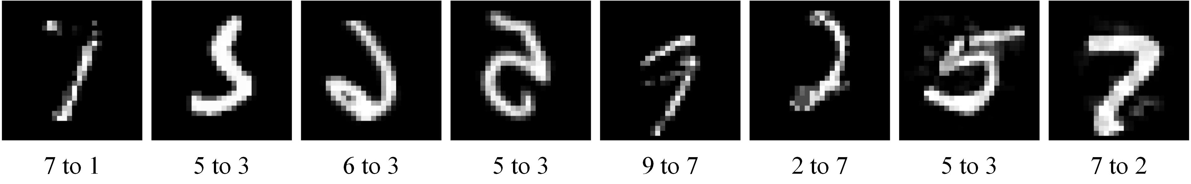
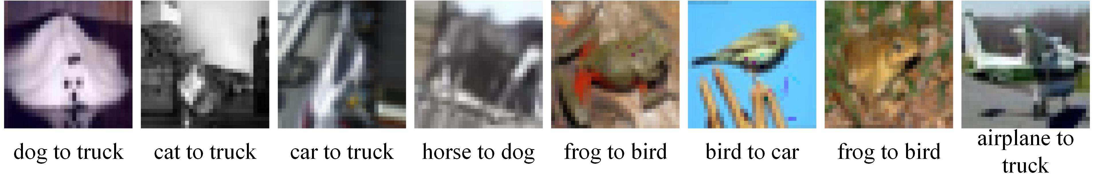
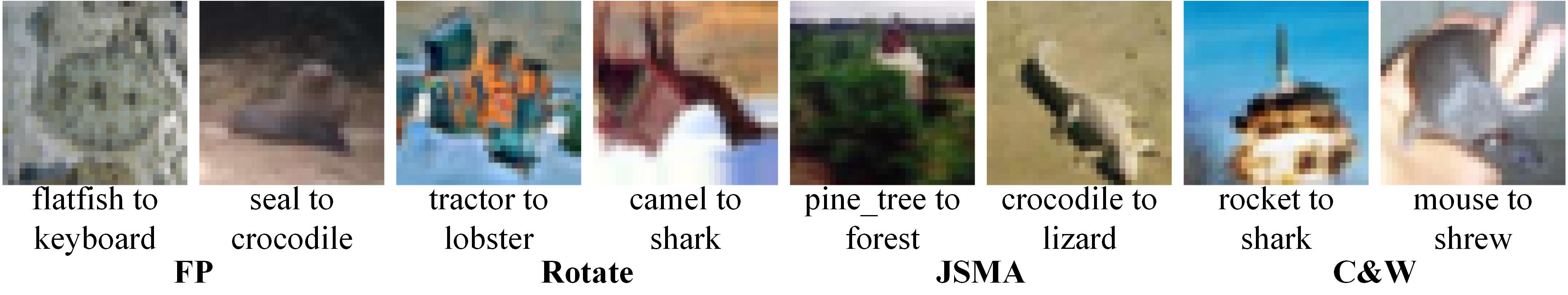
Figure 3: The visualization of test cases with high prioritization (i.e. FP, Rotate, JSMA and C&W). The first row is from MNIST, second row is from CIFAR-10 and third row is from CIFAR-100.

Qualitative analysis. The visualization of t-SNE is the first row of Fig. 4 for qualitative analysis. Intuitively, the features of Confidence and Embedding are confused, and the distances between different types are relatively close. In PRIMA, Clean and FP are close in distance, JSMA and C&W are close in distance, and Rotate is in the middle between natural and adversarial cases. This shows that although PRIMA can distinguish between FP and adversarial cases, it is difficult to distinguish between Clean and FP cases. In ActGraph, Rotate and Clean are distinguished, and most of the FP and Rotate overlap, only a few FP and Clean intersect, and the distance between JSMA and C&W is also farther than PRIMA. This shows that the center node feature of ActGraph not only has better prioritization performance for adversarial cases, but also has better prioritization effect on natural cases and FP cases than existing methods.

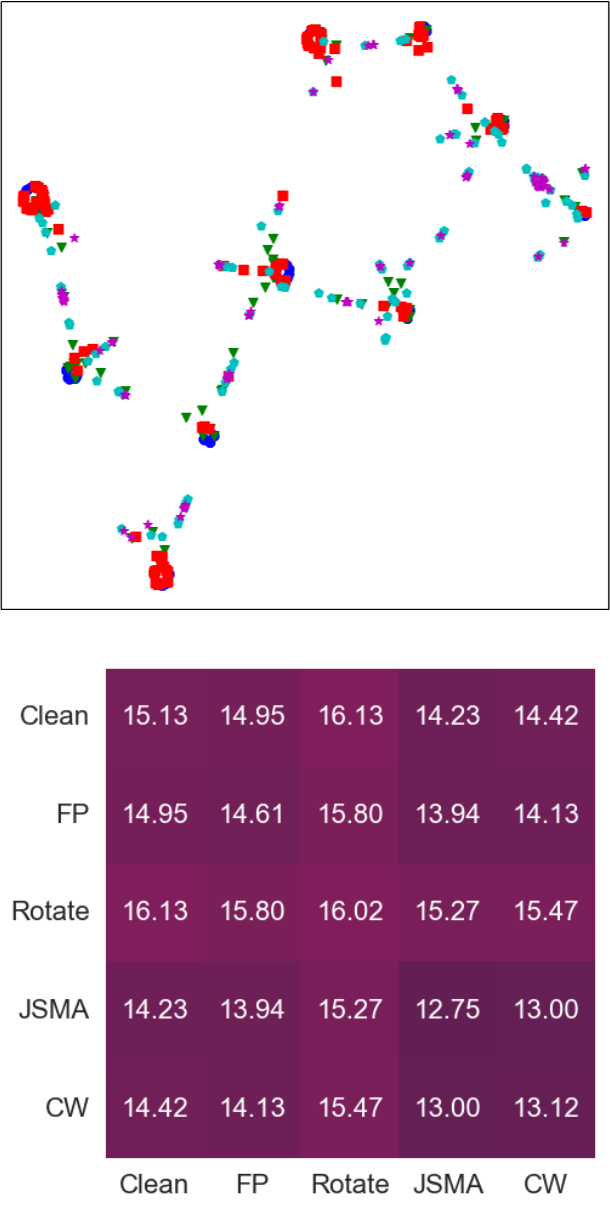
(a) Confidence

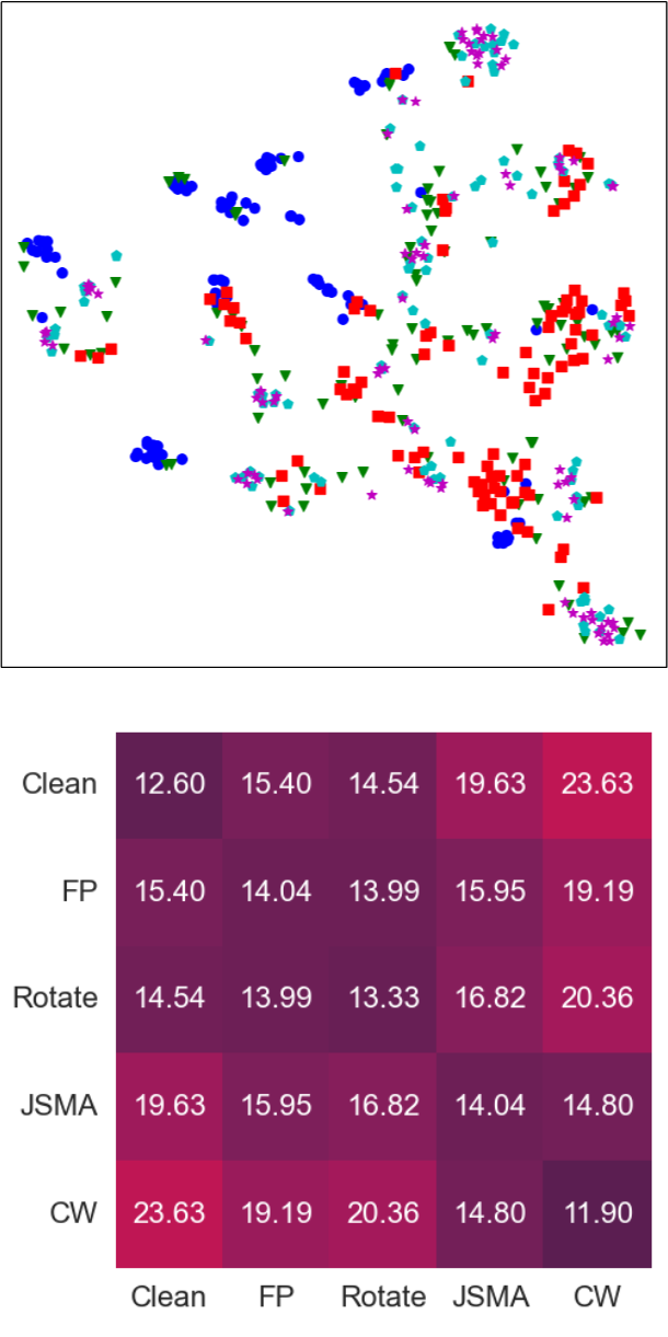
(b) Embedding

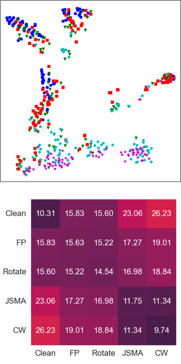
(c) PRIMA

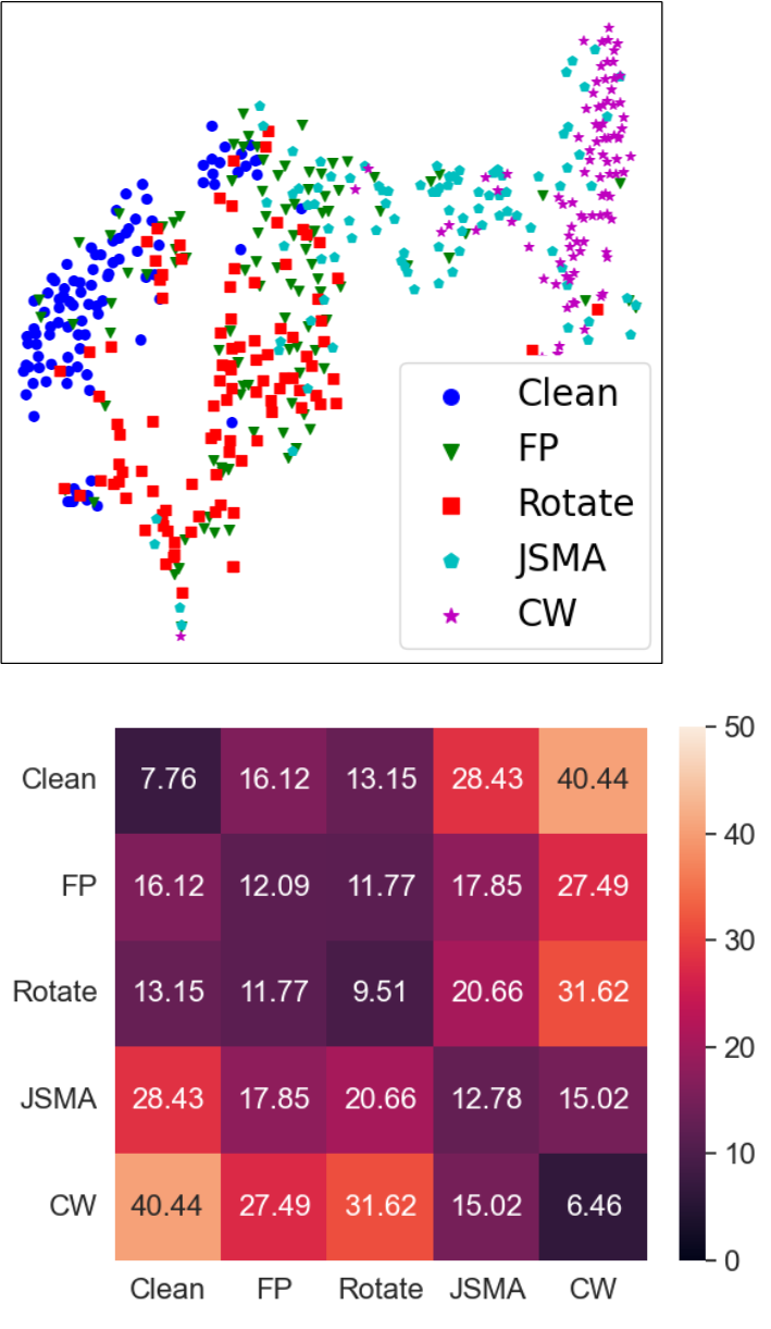
(d) ActGraph

Figure 4: The t-SNE and heatmap visualization. (a) Confidence is the output from the DNN confidence layer. (b) Embedding is the output from the last hidden layer of the DNN. (c) PRIMA represents the mutation feature from the PRIMA method. (d) ActGraph represents the center node feature. The number of cases of each type is 200. It is a VGG16 trained on CIFAR-10.

Quantitative analysis. We calculate intra-class and inter-class distances on the t-SNE for five types of cases, represented by the heatmap, for quantitative analysis, where the distance measure used Euclidean distance. The heat map is the second row of Fig. 4. For intra-class distance, ActGraph is 6.46$\sim$12.78. Except JSMA, the intra-class distance of ActGraph is smaller than other methods. For inter-class distance, intuitively, the distance between natural cases (Clean, FP and Rotate) and adversarial cases (JSMA and C&W) of ActGraph is all the farthest, with the farthest distance being 40.44, which is 1.54$\sim$2.80 times of the other three methods. This shows that ActGraph can distinguish natural samples from adversarial samples better than other methods. In addition, the distance from FP to Clean of ActGraph is 16.12, the distance from FP to Rotate is 11.77, and the difference is 4.35, while the difference of Confidence is -0.85, Embedding is 1.41, and PRIMA is 0.61. This shows that the FP of ActGraph is closer to Rotate and farther from Clean, and the effect of prioritization will be better. Also, ActGraph’s JSMA to C&W distance is farther than other methods.

Answer to RQ3: ActGraph has smaller intra-class distances and larger inter-class distances than the baseline methods. For inter-class distances, the maximum inter-class distance of ActGraph is 1.54$\sim$2.80 times that of the baseline methods, and the average inter-class distance of ActGraph is 1.12$\sim$1.36 times that of the baseline methods. For inter-class distances, the minimum inter-class distance of the baseline methods are 1.52$\sim$2.04 times that of ActGraph and the average inter-class distance are 1.28$\sim$1.47 times that of ActGraph.

4.5 Sensitivity Analysis of Parameters

In this section, we find the answer to RQ4. We analyze the influence of the size of trainset and training parameters of ActGraph.

Implementation details. (1) We set RAUC-100 as the evaluation metric. (2) It is a VGG16 trained on CIFAR-10. (3) The type of trainset and testset are both Mix.

Influence of trainset size. The result shows in Fig. 5. DeepGini and MCP are unsupervised methods, so are not affected by the size of the trainset. In LeNet-5 and VGG (VGG16 and VGG19), ActGraph exhibits the best prioritization performance, and the performance increases with the size of the dataset. In ResNet18, ActGraph performs better than most baseline algorithms. Importantly, ActGraph is less affected by changes in trainset size, while the remaining three baseline algorithms (i.e. PRIMA, DSA and Act) are more affected by changes in trainset size. This shows that ActGraph can learn effective features from a small number of cases.

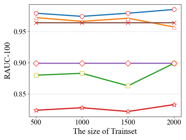
(a) LeNet-5

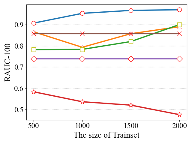
(b) VGG16

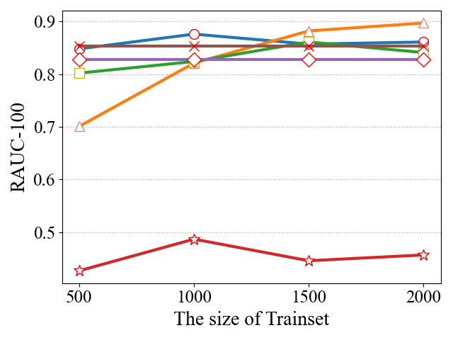
(c) ResNet18

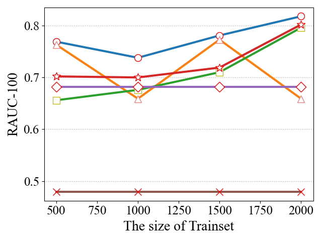
(d) VGG19

Figure 5: Influence of different size of trainset.

Influence of training parameters. We investigate the influence of main parameters in ActGraph, including Max depth (the maximum tree depth for each XGBoost model), Colsample bytree (the sampling ratio of columns of features when constructing each tree) and Learning rate (the boosting learning rate) in the XGBoost ranking algorithm. Fig. 6 shows the effectiveness of ActGraph under different parameter settings in RAUC-100 across the four models. We found that, ActGraph performs stably under different parameter settings and our default settings are proper.

Figure 6: Influence of hyperparameters in ActGraph.

Answer to RQ4: For the trainset size, we set four scenarios ranging from 500 to 2,000. ActGraph has stable performance and increases with the increase of the trainset size. For training hyperparameters, ActGraph is also stable. These results indicate that our previous parameter settings are appropriate.

4.6 Time Complexity

In this section, we find the answer to RQ5, referring to the prioritization time cost.

Implementation details. We measure average running time for ranking 10,000 test cases by ActGraph and baselines. We run each method for 5 times, and the average is identified as the final result.

Results and analysis. Firstly, we theoretically analyze the complexity of ActGraph according to different steps.

The time complexity of ActGraph includes acquiring activation values of multi-layer neurons, calculating $ap$, calculating $nf$ and calculating cnf, so its time complexity is

$$T\sim O(t\times V)+O(t\times E)+O(t\times E)+O(t\times E)\sim O(t\times E)$$ (16)

where $t$ is the number of samples, $V$ is the number of neurons, and $E$ is the number of edges between neurons.

Further, we analyze the efficiency of ActGraph from the real running time. According to the Table 5, the running time of ActGraph is acceptable, the time cost of ActGraph increases due to the increase of the total number of neurons and edges. In general, ActGraph is much faster than PRIMA, but is inferior to other methods. The reason is that we search more layers and neurons. Besides, ActGraph calculates the weighted edges between neurons, and calculates the center node features in the activation graph. PRIMA runs on average 50 times longer than ActGraph.

Table 5: Time (seconds) taken to prioritize 10,000 test cases

Datasets	Models	Methods
		DeepGini	PRIMA	Act	MCP	DSA	ActGraph
MNIST	LeNet-5	0.662	8049.53	0.642	0.626	11.59	103.69
CIFAR-10	VGG16	1.274	10864.19	1.115	1.465	19.09	246.26
	ResNet18	1.843	14516.53	1.735	2.444	37.36	306.44
CIFAR-100	VGG19	1.380	15461.26	1.367	1.705	19.00	291.05

Answer to RQ5: The average running time for ActGraph to prioritize 10,000 cases is about four minutes, which is acceptable.

5 THREATS TO VALIDITY

The depth of the graph. We explain why $K$=4 and take only two layers of cnf in Section 3.5. Too large $K$ value (more than 4) and the layer number of cnf (more than 2) will not only increase the time cost, but also introduce noise from the shallow layer. And the value of $K$ too small to obtain the valid cnf value. Therefore, it is appropriate to set $K$=4, which is also confirmed by the comprehensive experimental results.

Time cost. The time cost of ActGraph may be affected by the neuron number of the DNN. We demonstrate that the ActGraph’s runtime is acceptable by applying three popular DNN models with significant differences in the number of neurons.

Access to DNNs. ActGraph is a white-box method of prioritizing test cases. It needs to access the DNN for model weight parameters and deep activation of test cases. It is widely accepted that DNN testing could have full knowledge of the target model in software engineering.

6 CONCLUSIONS

Aiming at the problems of limited application scenarios and high time cost of existing test case prioritization methods, we propose a test case prioritization method based on the DNN activation graph, named ActGraph. We observe that the activation graphs of cases that trigger model vulnerabilities different from those of normal cases significantly. Motivated by it, ActGraph extracts the node features and adjacency matrix of test cases by building an activation graph, and uses the message passing mechanism to aggregate node features and adjacency matrix to obtain more effective center node features for test case prioritization. Extensive experiments have verified the effectiveness of ActGraph, which outperforms the SOTA method in both natural and adversarial scenarios, especially in RAUC-100 ($\sim\times$1.40). And when the number of test cases is 10,000, the actual running time of the SOTA method is 50 times that of ActGraph. The experiments show that ActGraph has significantly better performance in terms of effectiveness, generalizability, and efficiency.

In the future, we will improve our ActGraph approach and apply it to more popular tasks and models, such as the transformer model for natural language processing and the long short-term memory model for time series forecasting.

References

-
[1]
H. Zhang, X. Ma, Misleading
attention and classification: An adversarial attack to fool object detection
models in the real world, Comput. Secur. 122 (2022) 102876.
doi:10.1016/j.cose.2022.102876.
URL https://doi.org/10.1016/j.cose.2022.102876 -
[2]
Y. Duan, X. Zhou, J. Zou, J. Qiu, J. Zhang, Z. Pan,
Mask-guided noise
restriction adversarial attacks for image classification, Comput. Secur. 100
(2021) 102111.
doi:10.1016/j.cose.2020.102111.
URL https://doi.org/10.1016/j.cose.2020.102111 -
[3]
A. A. Alhogail, A. Alsabih,
Applying machine learning
and natural language processing to detect phishing email, Comput. Secur. 110
(2021) 102414.
doi:10.1016/j.cose.2021.102414.
URL https://doi.org/10.1016/j.cose.2021.102414 -
[4]
K. Kim, J. S. Kim, S. Jeong, J. Park, H. K. Kim,
Cybersecurity for
autonomous vehicles: Review of attacks and defense, Comput. Secur. 103
(2021) 102150.
doi:10.1016/j.cose.2020.102150.
URL https://doi.org/10.1016/j.cose.2020.102150 - [5] D. T. Danny Yadron, Tesla driver dies in first fatal crash while using autopilot mode, https://www.theguardian.com/technology/2016/jun/30/tesla-autopilot-death-self-driving-car-elon-musk, 2016.
-
[6]
K. Pei, Y. Cao, J. Yang, S. Jana,
Deepxplore: Automated whitebox
testing of deep learning systems, in: Proceedings of the 26th Symposium on
Operating Systems Principles, Shanghai, China, October 28-31, 2017, ACM,
2017, pp. 1–18.
doi:10.1145/3132747.3132785.
URL https://doi.org/10.1145/3132747.3132785 -
[7]
J. Guo, Y. Jiang, Y. Zhao, Q. Chen, J. Sun,
Dlfuzz: differential fuzzing
testing of deep learning systems, in: G. T. Leavens, A. Garcia, C. S.
Pasareanu (Eds.), Proceedings of the 2018 ACM Joint Meeting on European
Software Engineering Conference and Symposium on the Foundations of Software
Engineering, ESEC/SIGSOFT FSE 2018, Lake Buena Vista, FL, USA, November
04-09, 2018, ACM, 2018, pp. 739–743.
doi:10.1145/3236024.3264835.
URL https://doi.org/10.1145/3236024.3264835 -
[8]
A. Odena, C. Olsson, D. G. Andersen, I. J. Goodfellow,
Tensorfuzz: Debugging
neural networks with coverage-guided fuzzing, in: K. Chaudhuri,
R. Salakhutdinov (Eds.), Proceedings of the 36th International Conference on
Machine Learning, ICML 2019, 9-15 June 2019, Long Beach, California, USA,
Vol. 97 of Proceedings of Machine Learning Research, PMLR, 2019, pp.
4901–4911.
URL http://proceedings.mlr.press/v97/odena19a.html -
[9]
Y. Tian, K. Pei, S. Jana, B. Ray,
Deeptest: automated testing of
deep-neural-network-driven autonomous cars, in: M. Chaudron, I. Crnkovic,
M. Chechik, M. Harman (Eds.), Proceedings of the 40th International
Conference on Software Engineering, ICSE 2018, Gothenburg, Sweden, May 27 -
June 03, 2018, ACM, 2018, pp. 303–314.
doi:10.1145/3180155.3180220.
URL https://doi.org/10.1145/3180155.3180220 -
[10]
L. Ma, F. Juefei-Xu, F. Zhang, J. Sun, M. Xue, B. Li, C. Chen, T. Su, L. Li,
Y. Liu, J. Zhao, Y. Wang,
Deepgauge: multi-granularity
testing criteria for deep learning systems, in: M. Huchard,
C. Kästner, G. Fraser (Eds.), Proceedings of the 33rd ACM/IEEE
International Conference on Automated Software Engineering, ASE 2018,
Montpellier, France, September 3-7, 2018, ACM, 2018, pp. 120–131.
doi:10.1145/3238147.3238202.
URL https://doi.org/10.1145/3238147.3238202 -
[11]
Y. Feng, Q. Shi, X. Gao, J. Wan, C. Fang, Z. Chen,
Deepgini: prioritizing massive
tests to enhance the robustness of deep neural networks, in: S. Khurshid,
C. S. Pasareanu (Eds.), ISSTA ’20: 29th ACM SIGSOFT International
Symposium on Software Testing and Analysis, Virtual Event, USA, July 18-22,
2020, ACM, 2020, pp. 177–188.
doi:10.1145/3395363.3397357.
URL https://doi.org/10.1145/3395363.3397357 -
[12]
W. Shen, Y. Li, L. Chen, Y. Han, Y. Zhou, B. Xu,
Multiple-boundary clustering
and prioritization to promote neural network retraining, in: 35th IEEE/ACM
International Conference on Automated Software Engineering, ASE 2020,
Melbourne, Australia, September 21-25, 2020, IEEE, 2020, pp. 410–422.
doi:10.1145/3324884.3416621.
URL https://doi.org/10.1145/3324884.3416621 -
[13]
J. Kim, R. Feldt, S. Yoo,
Guiding deep learning system
testing using surprise adequacy, in: J. M. Atlee, T. Bultan, J. Whittle
(Eds.), Proceedings of the 41st International Conference on Software
Engineering, ICSE 2019, Montreal, QC, Canada, May 25-31, 2019, IEEE /
ACM, 2019, pp. 1039–1049.
doi:10.1109/ICSE.2019.00108.
URL https://doi.org/10.1109/ICSE.2019.00108 -
[14]
T. Byun, V. Sharma, A. Vijayakumar, S. Rayadurgam, D. D. Cofer,
Input prioritization for
testing neural networks, in: IEEE International Conference On Artificial
Intelligence Testing, AITest 2019, Newark, CA, USA, April 4-9, 2019, IEEE,
2019, pp. 63–70.
doi:10.1109/AITest.2019.000-6.
URL https://doi.org/10.1109/AITest.2019.000-6 -
[15]
Z. Wang, H. You, J. Chen, Y. Zhang, X. Dong, W. Zhang,
Prioritizing test inputs
for deep neural networks via mutation analysis, in: 43rd IEEE/ACM
International Conference on Software Engineering, ICSE 2021, Madrid, Spain,
22-30 May 2021, IEEE, 2021, pp. 397–409.
doi:10.1109/ICSE43902.2021.00046.
URL https://doi.org/10.1109/ICSE43902.2021.00046 -
[16]
H. Zhu, P. A. V. Hall, J. H. R. May,
Software unit test coverage and
adequacy, ACM Comput. Surv. 29 (4) (1997) 366–427.
doi:10.1145/267580.267590.
URL https://doi.org/10.1145/267580.267590 -
[17]
Y. K. Malaiya, M. N. Li, J. M. Bieman, R. Karcich,
Software reliability growth
with test coverage, IEEE Trans. Reliab. 51 (4) (2002) 420–426.
doi:10.1109/TR.2002.804489.
URL https://doi.org/10.1109/TR.2002.804489 -
[18]
C. Cadar, D. Dunbar, D. R. Engler,
KLEE:
unassisted and automatic generation of high-coverage tests for complex
systems programs, in: R. Draves, R. van Renesse (Eds.), 8th USENIX
Symposium on Operating Systems Design and Implementation, OSDI 2008,
December 8-10, 2008, San Diego, California, USA, Proceedings, USENIX
Association, 2008, pp. 209–224.
URL http://www.usenix.org/events/osdi08/tech/full_papers/cadar/cadar.pdf -
[19]
Z. Li, X. Ma, C. Xu, C. Cao,
Structural coverage
criteria for neural networks could be misleading, in: A. Sarma, L. Murta
(Eds.), Proceedings of the 41st International Conference on Software
Engineering: New Ideas and Emerging Results, ICSE (NIER) 2019, Montreal,
QC, Canada, May 29-31, 2019, IEEE / ACM, 2019, pp. 89–92.
doi:10.1109/ICSE-NIER.2019.00031.
URL https://doi.org/10.1109/ICSE-NIER.2019.00031 -
[20]
F. Harel-Canada, L. Wang, M. A. Gulzar, Q. Gu, M. Kim,
Is neuron coverage a
meaningful measure for testing deep neural networks?, in: P. Devanbu, M. B.
Cohen, T. Zimmermann (Eds.), ESEC/FSE ’20: 28th ACM Joint European
Software Engineering Conference and Symposium on the Foundations of Software
Engineering, Virtual Event, USA, November 8-13, 2020, ACM, 2020, pp.
851–862.
doi:10.1145/3368089.3409754.
URL https://doi.org/10.1145/3368089.3409754 -
[21]
Y. Dong, P. Zhang, J. Wang, S. Liu, J. Sun, J. Hao, X. Wang, L. Wang, J. S.
Dong, D. Ting, There is limited
correlation between coverage and robustness for deep neural networks, CoRR
abs/1911.05904.
arXiv:1911.05904.
URL http://arxiv.org/abs/1911.05904 -
[22]
N. Carlini, D. A. Wagner, Towards
evaluating the robustness of neural networks, in: 2017 IEEE Symposium on
Security and Privacy, SP 2017, San Jose, CA, USA, May 22-26, 2017, IEEE
Computer Society, 2017, pp. 39–57.
doi:10.1109/SP.2017.49.
URL https://doi.org/10.1109/SP.2017.49 -
[23]
Y. LeCun, L. Bottou, Y. Bengio, P. Haffner,
Gradient-based learning applied to
document recognition, Proc. IEEE 86 (11) (1998) 2278–2324.
doi:10.1109/5.726791.
URL https://doi.org/10.1109/5.726791 -
[24]
J. Gilmer, S. S. Schoenholz, P. F. Riley, O. Vinyals, G. E. Dahl,
Neural message passing
for quantum chemistry, in: D. Precup, Y. W. Teh (Eds.), Proceedings of the
34th International Conference on Machine Learning, ICML 2017, Sydney, NSW,
Australia, 6-11 August 2017, Vol. 70 of Proceedings of Machine Learning
Research, PMLR, 2017, pp. 1263–1272.
URL http://proceedings.mlr.press/v70/gilmer17a.html -
[25]
T. Liu, Learning to rank for
information retrieval, in: F. Crestani, S. Marchand-Maillet, H. Chen,
E. N. Efthimiadis, J. Savoy (Eds.), Proceeding of the 33rd International
ACM SIGIR Conference on Research and Development in Information
Retrieval, SIGIR 2010, Geneva, Switzerland, July 19-23, 2010, ACM, 2010,
p. 904.
doi:10.1145/1835449.1835676.
URL https://doi.org/10.1145/1835449.1835676 -
[26]
Z. Li, X. Ma, C. Xu, C. Cao, J. Xu, J. Lü,
Boosting operational DNN
testing efficiency through conditioning, in: M. Dumas, D. Pfahl, S. Apel,
A. Russo (Eds.), Proceedings of the ACM Joint Meeting on European Software
Engineering Conference and Symposium on the Foundations of Software
Engineering, ESEC/SIGSOFT FSE 2019, Tallinn, Estonia, August 26-30, 2019,
ACM, 2019, pp. 499–509.
doi:10.1145/3338906.3338930.
URL https://doi.org/10.1145/3338906.3338930 -
[27]
J. Chen, Z. Wu, Z. Wang, H. You, L. Zhang, M. Yan,
Practical accuracy estimation for
efficient deep neural network testing, ACM Trans. Softw. Eng. Methodol.
29 (4) (2020) 30:1–30:35.
doi:10.1145/3394112.
URL https://doi.org/10.1145/3394112 -
[28]
W. Ma, M. Papadakis, A. Tsakmalis, M. Cordy, Y. L. Traon,
Test selection for deep learning
systems, ACM Trans. Softw. Eng. Methodol. 30 (2) (2021) 13:1–13:22.
doi:10.1145/3417330.
URL https://doi.org/10.1145/3417330 -
[29]
Y. Chen, Z. Wang, D. Wang, Y. Yao, Z. Chen,
Behavior pattern-driven test
case selection for deep neural networks, in: IEEE International Conference
On Artificial Intelligence Testing, AITest 2019, Newark, CA, USA, April 4-9,
2019, IEEE, 2019, pp. 89–90.
doi:10.1109/AITest.2019.000-2.
URL https://doi.org/10.1109/AITest.2019.000-2 -
[30]
Z. Li, X. Ma, C. Xu, J. Xu, C. Cao, J. Lu,
Operational calibration:
debugging confidence errors for dnns in the field, in: P. Devanbu, M. B.
Cohen, T. Zimmermann (Eds.), ESEC/FSE ’20: 28th ACM Joint European
Software Engineering Conference and Symposium on the Foundations of Software
Engineering, Virtual Event, USA, November 8-13, 2020, ACM, 2020, pp.
901–913.
doi:10.1145/3368089.3409696.
URL https://doi.org/10.1145/3368089.3409696 -
[31]
G. Naitzat, A. Zhitnikov, L. Lim,
Topology of deep neural
networks, J. Mach. Learn. Res. 21 (2020) 184:1–184:40.
URL http://jmlr.org/papers/v21/20-345.html -
[32]
D. Filan, S. Casper, S. Hod, C. Wild, A. Critch, S. Russell,
Clusterability in neural networks,
CoRR abs/2103.03386.
arXiv:2103.03386.
URL https://arxiv.org/abs/2103.03386 -
[33]
B. Rieck, M. Togninalli, C. Bock, M. Moor, M. Horn, T. Gumbsch, K. M.
Borgwardt, Neural
persistence: A complexity measure for deep neural networks using algebraic
topology, in: 7th International Conference on Learning Representations,
ICLR 2019, New Orleans, LA, USA, May 6-9, 2019, OpenReview.net, 2019.
URL https://openreview.net/forum?id=ByxkijC5FQ -
[34]
F. Vahedian, R. Li, P. Trivedi, D. Jin, D. Koutra,
Convolutional neural network
dynamics: A graph perspective, CoRR abs/2111.05410.
arXiv:2111.05410.
URL https://arxiv.org/abs/2111.05410 -
[35]
Y. Zhao, H. Zhang,
Quantitative performance
assessment of CNN units via topological entropy calculation, in: The Tenth
International Conference on Learning Representations, ICLR 2022, Virtual
Event, April 25-29, 2022, OpenReview.net, 2022.
URL https://openreview.net/forum?id=xFOyMwWPkz -
[36]
T. Chen, C. Guestrin, Xgboost:
A scalable tree boosting system, in: B. Krishnapuram, M. Shah, A. J.
Smola, C. C. Aggarwal, D. Shen, R. Rastogi (Eds.), Proceedings of the 22nd
ACM SIGKDD International Conference on Knowledge Discovery and Data
Mining, San Francisco, CA, USA, August 13-17, 2016, ACM, 2016, pp.
785–794.
doi:10.1145/2939672.2939785.
URL https://doi.org/10.1145/2939672.2939785 - [37] A. Krizhevsky, Learning multiple layers of features from tiny images, Master’s thesis, University of Tront.
-
[38]
K. Simonyan, A. Zisserman, Very deep
convolutional networks for large-scale image recognition, in: Y. Bengio,
Y. LeCun (Eds.), 3rd International Conference on Learning Representations,
ICLR 2015, San Diego, CA, USA, May 7-9, 2015, Conference Track Proceedings,
2015.
URL http://arxiv.org/abs/1409.1556 -
[39]
K. He, X. Zhang, S. Ren, J. Sun,
Deep residual learning for image
recognition, in: 2016 IEEE Conference on Computer Vision and Pattern
Recognition, CVPR 2016, Las Vegas, NV, USA, June 27-30, 2016, IEEE
Computer Society, 2016, pp. 770–778.
doi:10.1109/CVPR.2016.90.
URL https://doi.org/10.1109/CVPR.2016.90 -
[40]
N. Papernot, P. D. McDaniel, S. Jha, M. Fredrikson, Z. B. Celik, A. Swami,
The limitations of deep
learning in adversarial settings, in: IEEE European Symposium on Security
and Privacy, EuroS&P 2016, Saarbrücken, Germany, March 21-24, 2016,
IEEE, 2016, pp. 372–387.
doi:10.1109/EuroSP.2016.36.
URL https://doi.org/10.1109/EuroSP.2016.36