Entanglement and non-classical states of light in a strong-laser driven solid-state system

Abstract

The development of sources delivering non-classical states of light is one of the main needs for applications of optical quantum information science. Here, we demonstrate the generation of non-classical states of light using strong-laser fields driving a solid-state system, by using the process of high-order harmonic generation, where an electron tunnels out of the parent site and, later on, recombines on it emitting high-order harmonic radiation, at the expense of affecting the driving laser field. Since in solid-state systems the recombination of the electron can be delocalized along the material, the final state of the electron determines how the electromagnetic field gets affected because of the laser-matter interaction, leading to the generation of entanglement between the electron and the field. These features can be enhanced by applying conditioning operations, i.e., quantum operations based on the measurement of high-harmonic radiation. We study non-classical features present in the final quantum optical state, and characterize the amount of entanglement between the light and the electrons in the solid. The work sets the foundation for the development of compact solid-state-based non-classical light sources using strong-field physics.

Quantum optics stands as one of the most promising natural platforms for the development of practical applications of quantum information science [1, 2, 3], light being the main carrier of information. To pursue such developments, non-classical states of light are needed, i.e. those which are necessarily described by quantum electrodynamical tools [4]. Many of the currently available non-classical light sources rely on nonlinear interactions between light and matter [5]. Among the most striking examples of nonlinear interactions, is the process of high-order harmonic generation (HHG) [6, 7, 8, 9]. Here, a pulsed and strong-laser field interacts with matter leading to the generation of radiation, emitted as a periodic series of ultrashort comb of harmonics of the driving laser that spans dozens, hundreds or even thousands of harmonic orders [10]. Because of these features, HHG has found numerous applications in attosecond science (cf. [11, 12, 13]), nonlinear XUV optics (cf. [14, 15, 16, 17, 18, 19, 20, 21]), and high-resolution spectroscopy (cf. [22, 23]). In these, a semiclassical theoretical description of HHG, where light is treated classically while the matter system quantum mechanically [24, 12], is enough to reproduce the experimental results, although leaving unexploited the potential of strong-field physics towards quantum optics [25]. Recently, atomic-HHG processes were studied under a quantum optical framework, proving theoretically and experimentally the generation of non-classical states of light [26, 27, 28, 29] spanning from the infrared (IR) up to the extreme ultraviolet (XUV) [30]. The essential ingredient behind the findings of Refs. [26, 27, 28, 30, 31] was the conditioning operation, i.e., restricting measurements of the outgoing radiation to instances in which harmonics were generated.

In this work, we extend the techniques that have been developed so far for generating non-classical states of light with atomic-HHG processes, to solid-state systems. In atoms, the process behind HHG is resumed in the so-called three-step model [32, 33, 34, 24], in which an electron (i) is extracted from the atom, (ii) accelerates in the continuum driven by the laser field, and (iii) recollides with the parent ion releasing the gained kinetic energy in form of coherent high-frequency radiation. For solids [11, 35, 36, 37], the process underlying the generation of harmonic radiation becomes more complex [38, 39]. Besides the transitions between valence and conduction bands (interband transitions), which find their analogy in gaseous-HHG with the ionization and recombination steps, the electron undergoes excitations within the same band (intraband transitions). This increases the delocalization of the electron, allowing it to recombine, in the emission step later on, with a different site from the one in which it had initially started the dynamics. These additional processes, previously studied under a semiclassical framework [38, 40, 41], leave their fingerprints in the final quantum optical state even in the regime of weak delocalization, which we consider here. Specifically, the recombination of the electron with a different site from which it was promoted to the conduction band, affects differently the optical state compared to the on-site recombination, leading to electron position-light entanglement. This non-classical effect occurs without any need for conditioning, which might augment the non-classical features, and lead to the generation of coherent state superpositions, as those found in Refs. [26, 27, 30, 28]. In Ref. [42], the authors studied, from a quantum optical perspective, the effect of intraband transitions within the conduction band on the final quantum optical state, revealing the presence of non-classical states of light after the measurement of harmonic radiation. Finally, if valence intraband dynamics are very fast, such that recombination may occur anywhere in the solid with a random phase associated, they lead to decoherence of harmonics and hinders the phase matching efficiency, as discussed recently in Ref. [43].

RESULTS

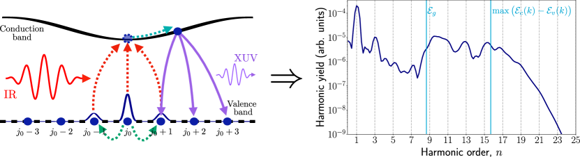
Figure 1: Pictorial representation of the high-order harmonic generation process in solid-state systems. An electron, initially placed at site $j_{0}$, which can perform intraband transitions to other Wannier sites (green dotted curves), gets excited to the conduction band (red dotted curves). Driven by the input field, the electron accelerates in the conduction band (blue dotted curve) and eventually recombines with a given Wannier site of the valence band (purple solid curves). The energy acquired during its acceleration along the conduction band is emitted in the form of high-harmonic photons, whose spectral distribution is typically characterized by a plateau region ranging from the bandgap energy $\mathcal{E}_{g}$, up to the maximum energy difference between valence and conduction bands, i.e. $\max(\mathcal{E}_{c}(k)-\mathcal{E}_{v}(k))$, as shown in the plot located at the right hand side of the figure.

Quantum optical framework. In typical experimental realizations of intense laser-matter interactions with solid-state systems, a driving laser field of wavelength belonging to the mid-infrared (MIR) regime ($\lambda\sim 3-8$ $\mu$m), hits the target perpendicularly and generates harmonic radiation along the transmission path [44, 45]. Before the dynamics start, we describe the input electromagnetic field mode with a coherent state $\ket{\alpha_{L}}$, while all harmonic modes with a vacuum state $\ket{0_{\text{HH}}}=\bigotimes_{q=2}\ket{0_{q}}$ where $q\in\mathbbm{N}$ denotes the harmonic order. Regarding the solid, we assume it to be in its ground state, corresponding to a completely filled Fermi sea. However, we first solve the time-dependent Schrödinger equation for a single electron, and then phenomenologically treat the many-electron case. Thus, we characterize the initial state of our electron in the Wannier basis as $\ket{w_{v,j_{0}}}$ (such that $\innerproduct{w_{v,i}}{w_{v,j}}=\delta_{i,j}$), where the subscript $v$ denotes the band in which it is located (valence) and $j_{0}$ its initial site. It can be shown (Methods) that the evolution of the quantum optical state of the system projected onto a Wannier state $\ket{w_{v,j}}$, and neglecting the contributions coming from the conduction band, is given by

$$i\hbar\partialderivative{\ket{\Phi_{i}(t)}}{t}=\sum_{j}\mathbf{M}_{i,j}(t)\cdot\hat{\mathbf{E}}(t)\ket{\Phi_{j}(t)}\ \forall i\in\mathbbm{Z}.$$ (1)

Here, $\hbar$ is Planck’s constant, $\ket{\Phi_{i}(t)}$ is the quantum optical state when projected into Wannier state $\ket{w_{v,i}}$, $\mathbf{M}_{i,j}(t)$ are the matrix elements of the time-dependent dipole moment with respect to $\ket{w_{v,i}}$ and $\ket{w_{v,j}}$, and $\hat{\mathbf{E}}(t)$ is the time-dependent electric field operator. Considering solids for which the HHG process is localized, such that the electron occasionally ends the dynamics in, at most, its nearest-neighboring sites, we can write the solution to Eq. (1), up to first-order perturbation theory, as (Methods)

$$\ket{\Phi_{j_{0}}(t)}=e^{i\varphi(t)}\hat{D}_{1}(\alpha_{L})\hat{\mathcal{D}}\big{(}\bm{\chi}(t,t_{0})\big{)}\bigotimes_{q=1}\ket{0_{q}},$$ (2)

when $i=j_{0}$ in Eq. (1), and

$$\ket{\Phi_{\text{NN}}(t)} =-\dfrac{i}{\hbar}e^{i\varphi(t)}\hat{D}_{1}(\alpha_{L})\hat{\mathcal{D}}\big{(}\bm{\chi}(t,t_{0})\big{)}$$ (3)

$$\quad\times\int^{t}_{t_{0}}\differential t^{\prime}e^{-i\theta(t^{\prime})}\hat{\mathcal{D}}^{\dagger}\big{(}\bm{\chi}(t^{\prime},t_{0})\big{)}$$

$$\hskip 34.14322pt\times\big{(}\mathbf{M}_{i,j_{0}}(t^{\prime})\cdot\hat{\mathbf{E}}(t^{\prime})\big{)}\hat{\mathcal{D}}\big{(}\bm{\chi}(t^{\prime},t_{0})\big{)}\bigotimes_{q=1}\ket{0_{q}},$$

when $i=j_{0}\pm 1$ in 1D, or generally “nearest neighbors”, denoted NN. In Eqs. (2) and (3), $\varphi(t)$ and $\theta(t)$ are some phase factors (Methods), $\hat{D}_{q}(\cdot)$ is the displacement operator acting on mode $q$ [46, 47], $\hat{\mathcal{D}}(\bm{\chi}(t,t_{0}))=\prod_{q}\hat{D}_{q}(\chi_{q}(t,t_{0}))$ and $\chi_{q}(t,t_{0})$ is given by

$$\chi_{q}(t,t_{0})=-\dfrac{1}{\hbar}\int^{t}_{t_{0}}\differential t^{\prime}e^{iq\omega_{L}t^{\prime}}\mathbf{g}(\omega_{L})\cdot\mathbf{M}_{i,i}(t^{\prime}),$$ (4)

where we have taken into account that all Wannier sites are equivalent and, therefore, $\chi_{q}(t,t_{0})$ is independent of the Wannier site $i$. In these expressions, $\mathbf{g}(\omega_{L})$ arises from the expansion of the electric field operator into the quantized modes.

Electron position-light entanglement. The most important difference between the results for solids and atoms regarding the HHG process, is that in solids we encounter the possibility of electron position-light entanglement without the need for conditioning operations. We observe that the final Wannier site in which the electron ends up its dynamics, is crucial in determining the final quantum optical state. When valence intraband dynamics are slow on the time scale of the laser pulse duration, both initial and final sites are equal, and results are analogous to those found in atoms [26, 27, 28]: the different field modes get displaced a quantity $\chi_{q}(t,t_{0})$, corresponding to the Fourier transform of the time-dependent dipole moment averaged over $\ket{w_{v,j_{0}}}$, that determines the HHG spectrum (Fig. 1). When the electron is found in a different site from $j_{0}$, the quantum optical state of the system gets affected because of this extra interaction, accounted by $\mathbf{M}_{i,j_{0}}(t^{\prime})\cdot\hat{\mathbf{E}}(t^{\prime})$, describing a transition from the initial site $j_{0}$ to the final site $i$ (in our case $i=j_{0}\pm 1$) happening at time $t^{\prime}$. The dynamics at the new site lead to an extra displacement $\chi_{q}(t,t^{\prime})$ in each of the modes, indistinguishable from the one we get when recombination happens at site $j_{0}$, due to the equivalence between different Wannier sites. We note that the electron could potentially hop to other sites, although for the regime considered here, these contributions would be smaller than the ones already introduced, and can be treated with higher-order terms in a perturbation theory-based approach. When valence intraband dynamics are fast enough such that electrons can recombine at any site with a random phase, we get decoherence of HHG radiation and impossibility of efficient phase matching [43].

For a 1D lattice, the joint state of the system can be written as

$$\ket{\psi(t)}=\ket{w_{v,j_{0}}}\ket{\Phi_{j_{0}}(t)}+\sqrt{2}\ket{w_{v,\text{NN}}}\ket{\Phi_{\text{NN}}(t)},$$ (5)

where we defined $\ket{w_{v,\text{NN}}}=(1/\sqrt{2})(\ket{w_{v,j_{0}+1}}+\ket{w_{v,j_{0}-1}})$, and took into account that the quantum optical state $\ket{\Phi_{\text{NN}}(t)}$ is independent of the electron hopping to site $j_{0}+1$ or $j_{0}-1$ under the regime of weak delocalization.

If we denote by $f_{\rm c}$ the coordinate number of the lattice (i.e. $f_{\rm c}=2d$ in hypercubic lattices in $d$-dimensions, $f_{\rm c}=3$ for honeycomb lattice in 2D, $f_{\rm c}=6$ for triangular lattice in 2D), in arbitrary dimension we get

$$\ket{\psi(t)}=\ket{w_{v,j_{0}}}\ket{\Phi_{j_{0}}(t)}+\sqrt{f_{\rm c}}\ket{w_{v,\text{NN}}}\ket{\Phi_{\text{NN}}(t)},$$ (6)

where now $\ket{w_{v,\text{NN}}}=(1/\sqrt{f_{\rm c}})(\sum_{j\in\text{NN}}\ket{w_{v,j_{0}+j}})$.

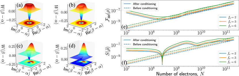
Figure 2: Wigner function representation, fidelity and entanglement for the many-electron case. In (a) to (d), we show the Wigner function distribution of the state after the conditioning for different values of $N$, specifically (a) $N=1\times 10^{7}$, (b) $N=1\times 10^{8}$, (c) $N=5\times 10^{8}$ and (d) $N=1\times 10^{9}$. We have used the terminology presented in Ref. [48], such that $\real(\beta-\alpha)=x$ and $\imaginary(\beta-\alpha)=p$ with $x$ and $p$ are the mean value of the quadrature operators $\hat{p}=(\hat{a}-\hat{a}^{\dagger})/(i\sqrt{2})$ and $\hat{x}=(\hat{a}+\hat{a}^{\dagger})/\sqrt{2}$. In (e) and (f) we show, respectively, the fidelity of the state in Eq. (7) with respect to the state $\big{\lvert}w_{v,\overline{\text{NN}}}\big{\rangle}$, and the entropy of entanglement $S(\tilde{\rho})$, with $\tilde{\rho}=\tr_{\text{field}}(\outerproduct{\psi(t)}{\psi(t)})$ for the dashed curves and $\tilde{\rho}=\tr_{\text{field}}(\outerproduct{\Psi_{\text{cond}}(t)}{\Psi_{\text{cond}}(t)})$ for the solid curves, when considering different coordinate numbers $f_{c}$, which correspond to a 1D lattice ($f_{c}=2$ in blue), a honeycomb lattice in 2D ($f_{c}=3$ in orange) and a triangular lattice in 2D ($f_{c}=6$ in green). In both plots, we consider the state before and after the conditioning operation is applied, which are respectively shown with the dashed and solid curves, respectively.

Phenomenological many-electron theory. Hitherto, we have only considered the single-electron dynamics. Under the assumption of having localized HHG processes, we can extend the solution given in Eq. (5) to the regime of $N$ independent and phase-matched electrons contributing to the process as (Methods)

$$\ket{\Psi(t)}=\ket{w_{v,\bm{j_{0}}}}\ket{\Phi_{\bm{j_{0}}}(t)}+\sqrt{f_{c}N}\big{\lvert}w_{v,\overline{\text{NN}}}\big{\rangle}\ket{\Phi_{\overline{\text{NN}}}(t)},$$ (7)

where $|\Phi_{\bm{j_{0}}}(t)\rangle$ and $|\Phi_{\overline{\text{NN}}}(t)\rangle$ differ from Eqs. (2) and (3) in that the displacement is given as $N\bm{\chi}(t,t_{0})$. In Eq. (7), $\bm{j_{0}}$ is an $N$-dimensional vector describing the initial Wannier site of the electrons, and $\big{\lvert}w_{v,\overline{\text{NN}}}\big{\rangle}=(1/\sqrt{f_{c}N})\sum_{\bm{j}\in\overline{\text{NN}}}\ket{w_{v,\bm{i}}}$ where $\overline{\text{NN}}:=\{\bm{j}:\bm{j_{0}}\pm(0_{1},\cdots,1_{i},\cdots,0_{N})\ \forall i\}$. The state presented in Eq. (7) has the structure of an entangled state, as recombination in different Wannier sites leads to different quantum optical components.

Conditioning on HHG. Current experimental implementations showed that, quantum operations relying on correlation measurements between the harmonics and part of the fundamental mode [49, 50, 26, 27, 30, 28], allow for the generation of non-classical states of light [26, 27, 30, 31, 28]. Mathematically, this operation can be written by means of the projective operator $\hat{P}_{\text{HHG}}=\mathbbm{1}-\outerproduct{\alpha}{\alpha}\otimes\outerproduct{0_{\text{HH}}}{0_{\text{HH}}}$, which we refer to as conditioning on HHG operation [30, 31]. Applying it onto Eq. (7), and further projecting with respect to the coherent state $\ket{\bm{\gamma}}=\bigotimes_{q\geq 2}\ket{\gamma_{q}}$ in which the harmonics are measured, leads

$$\ket{\Psi_{\text{cond}}(t)}=\innerproduct{\bm{\gamma}}{\Psi(t)}-\xi(\bm{\gamma},t)\ket{\alpha_{L}},$$ (8)

with $\xi(\bm{\gamma},t)=\innerproduct{\alpha,0_{\text{HH}}}{\Psi(t)}\innerproduct{\bm{\gamma}}{0_{\text{HH}}}$. Hereupon, we set $\gamma_{q}=\chi_{q}(t,t_{0})$.

In general, we have no knowledge about what site has the electron recombined in, and therefore the quantum optical state of the system is given as the mixed state $\hat{\rho}_{\text{field}}(t)=\tr_{\text{elec}}(\outerproduct{\Psi_{\text{cond}}(t)}{\Psi_{\text{cond}}(t)})$. In the following, we characterize two non-exclusive indications of non-classical behaviors: the presence of Wigner function negativities in $\hat{\rho}_{\text{field}}(t)$, and the presence of entanglement in $\ket{\Psi(t)}$ and $\ket{\Psi_{\text{cond}}(t)}$.

Non-classical properties in the many-electron regime. In the many-electron regime, we consider the case where intraband transitions within the valence band are either negligible, or weak. For HHG processes, it was shown that interband phenomena dominate in the HHG spectrum [51], which we consider in the computation of $\mathbf{M}_{i,j}(t)$ (Methods). We use ZnO as a solid system, for which the harmonic emission shows a weaker dependence with the field’s ellipticity compared to atoms [45], suggesting a small influence of delocalized recombination. We excite it with a linearly polarized laser along the $\Gamma-A$ direction, a sin²-shaped envelope, central wavelength $\lambda_{L}=3.25\ \mu\text{m}$, peak intensity $I_{0}=5\times 10^{11}\ \text{W/cm}^{2}$ and $\sim\!40\ \text{fs}$ of duration.

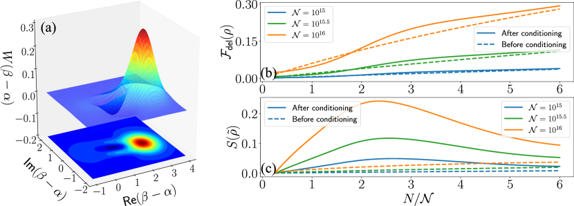
Figure 3: Wigner function representation, fidelity and entanglement for the many-electron case when reducing |$\bm{\chi(t,t_{0})}$|. In (a), we show the Wigner function distribution of the state after the conditioning for $N=4\times 10^{16}$. In (b) and (c) we show, respectively, the fidelity of the state in Eq. (7) with respect to the state $\big{\lvert}w_{v,\overline{\text{NN}}}\big{\rangle}$, and the entropy of entanglement. Here, the $x$ axis represents the number of electrons divided by a quantity $\mathcal{N}$, representing the order of magnitude in the number of electrons. In both plots we consider the state before and after the conditioning operation is applied, which are respectively shown with the dashed and solid curves, respectively.

Quantum state of the fundamental after conditioning on HHG. We study how the Wigner distribution of the quantum optical state in Eq. (8), varies when modifying the number of electrons $N$. First, we present the results obtained directly from the numerical evaluations, shown in Fig. 2 (a)-(d), where $N\in[1\times 10^{7},1\times 10^{9}]$ and $\absolutevalue{\bm{\chi}(t,t_{0})}\sim 10^{-3}-10^{-1}$. Similarly to atoms [26, 27, 30], the obtained Wigner distribution shifts from a displaced Fock state (Fig. 2 (a)), to an unbalanced superposition between two close coherent states (Fig. 2 (b) and (c)) until reaching a regime where one of the coherent states in the superposition dominates (Fig. 2 (d)). The Wigner distribution does not present striking differences with respect to those found for atomic systems. This is a consequence of the regime under which we are working, i.e., the dynamics within the valence band are practically negligible. However, note that the properties of $\bm{\chi}(t,t_{0})$ depend on factors such as the nature of the material, the direction along which gets excited, and the characteristics of the field (ellipticity, field intensity and frequency). Thus, if we consider the case where $N=4\times 10^{16}$, but where $\absolutevalue{\bm{\chi}(t,t_{0})}$ is drastically reduced, we get Wigner distributions as the one shown in Fig. 3 (a). Here, we distinguish two contributions: a big peak around $\text{Re}(\beta-\alpha)\simeq 2.8$, and a very small trough around the origin. While the former corresponds to the shifted part of the state (as in Fig. 2 (d)), the other contribution gets highlighted, as recombinations ending up in the nearest neighbor sites increase with $N$, introducing a small (but non-negligible) vacuum component. Between both, we get Wigner negativities arising from the quantum superposition of these two components.

Electron position-light entanglement. Here, we study the light-matter entanglement as a function of $N$ by computing the entropy of entanglement $S(\tilde{\rho}):=-\tr_{\text{elec}}(\tilde{\rho}\log_{2}(\tilde{\rho}))$, where $\tilde{\rho}(t)$ either represents $\tr_{\text{field}}(\outerproduct{\psi(t)}{\psi(t)})$ or $\tr_{\text{field}}(\outerproduct{\Psi_{\text{cond}}(t)}{\Psi_{\text{cond}}(t)})$, depending on whether it is computed before or after the conditioning. We compare the features of this entanglement measure with the ones obtained for the fidelity of $\ket{\psi(t)}$ and $\ket{\Psi_{\text{cond}}(t)}$ with respect to $|w_{v,\overline{\text{NN}}}\rangle$, i.e. $\mathcal{F}_{\text{del}}(\rho)=\text{tr}_{\text{field}}(\langle w_{v,\overline{\text{NN}}}|\hat{\rho}|w_{v,\overline{\text{NN}}}\rangle)$ with $\hat{\rho}=\outerproduct{\psi(t)}{\psi(t)}$ or $\hat{\rho}=\outerproduct{\Psi_{\text{cond}}(t)}{\Psi_{\text{cond}}(t)}$ depending on whether it is computed before or after the conditioning. The results for ZnO are shown in Fig. 2 (b) and (c) for $\mathcal{F}_{\text{del}}(\rho)$ and $S(\tilde{\rho})$, respectively. We observe that both quantities present very small values, as a consequence of the localized regime under which we are working. However, even in this range, there are some features to highlight. First, for $N\lesssim 2\times 10^{8}$ both the fidelity and the entanglement after the conditioning (solid curves) are bigger than before the conditioning (dashed curves). Here, $\absolutevalue{\bm{\chi}(t,t_{0})}$ is a small quantity ($\sim 10^{-2}$), allowing the conditioning to highlight contributions of the electron recombining in the nearest-neighbors (shown by the increase in fidelity compared to the situation without conditioning), increasing the value of $S(\tilde{\rho})$. At $N\simeq 2.5\times 10^{8}$, we observe an abrupt drop in $S(\tilde{\rho})$ after the conditioning, which is absent for $\mathcal{F}_{\text{del}}(\rho)$. Here, the quantum optical contributions arising from the $\lvert w_{\overline{\text{NN}}}\rangle$ term of Eq. (8), i.e. $\innerproduct{\bm{\gamma}}{\Phi_{\overline{\text{NN}}}(t)}-\xi(\bm{\gamma},t)\ket{\alpha_{L}}$, cancel each other, leaving the separable on-site contribution, and the observed drop in $S(\tilde{\rho})$. As $N$ grows, $\xi(\bm{\gamma},t)$ becomes smaller as $\absolutevalue{\bm{\chi}(t,t_{0})}$ gets bigger, since the overlap with the initial state is very small. In this regime, where conditioning does nothing, $\mathcal{F}_{\text{del}}(\rho)$ and $S(\tilde{\rho})$ for the state before and after the conditioning coincide. Note that these two quantities become bigger as the coordinate number $f_{c}$ increases. If the same analysis is done for the case where $N$ is increased to the order of $10^{16}$ while $\absolutevalue{\bm{\chi}(t,t_{0})}$ is drastically reduced, $S(\tilde{\rho})$ and $\mathcal{F}_{\text{del}}(\rho)$ get enhanced (Fig. 3 (b) and (c)). When $\absolutevalue{\bm{\chi}(t,t_{0})}\sim 10^{-1}$, we observe that $S(\tilde{\rho})\simeq 0.2$ for $N\simeq 2.2\times 10^{16}$, while $\mathcal{F}_{\text{del}}(\rho)\simeq 0.15$. For other values of $N$, we observe the same behaviour as presented in Figs. 2 (e) and (f): for $N<2.2\times 10^{16}$, $S(\tilde{\rho})$ drops to zero, which identifies with the huge dip observed in Fig. 2 (f), while below this value a small enhancement is observed, although not shown in this plot; for $N>2.2\times 10^{16}$, both $S(\tilde{\rho})$ and $\mathcal{F}_{\text{del}}(\rho)$ before and after the conditioning converge.

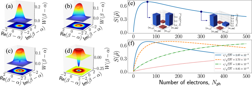
Figure 4: Wigner function representation and many-electron entanglement for the few-electron case. In (a) to (d), we show the Wigner function representation of the state after the conditioning for different values of $N$, specifically (a) $N=10$, (b) $N=40$, (c) $N=60$ and (d) $N=300$, while in all cases we have set $\epsilon/\sqrt{2N}=2.97\times 10^{-3}$, where we have considered a 1D lattice such that $f_{c}=1$. In (e) and (f) we show the entropy of entanglement as a function of the number of electrons. While in (e) we have set $\epsilon/\sqrt{2N}=2.97\times 10^{-3}$, in (f) we have considered different values of $\epsilon$ satisfying $\epsilon\sqrt{2N}\leq 0.3$. The histograms shown in the inset of (e) present the norm of the matrix elements $\lvert\matrixelement{w_{v,m}}{\tilde{\rho}}{w_{v,n}}\rvert$, with $\tilde{\rho}$ the state of the system once the partial trace with respect to the quantum optical degrees of freedom has been done.

Non-classical properties in the few-electron regime. Here, we consider the few-electron regime and, in counterpart, we increase the intraband dynamics within the valence band by defining a perturbation parameter $\epsilon$ (Methods) satisfying $\epsilon\sqrt{f_{c}N}<0.3$. We note that an increase of the valence band dynamics corresponds to an enhancement of the hopping potential between sites $I_{v}$, which is related with the curvature of the valence band (Methods). Therefore, the localized regime corresponds to solids for which the valence band is essentially flat, i.e. $I_{v}\lesssim 10^{-2}$, when excited with pulses of $\sim 40\ \text{fs}$ of duration.

Fig. 4 (a)-(d) shows the Wigner function after the conditioning, respectively for $N=10,40,60,300$, for which $\absolutevalue{\bm{\chi}(t,t_{0})}\sim 10^{-8}-10^{-6}$, while setting $\epsilon/\sqrt{2N}=2.97\times 10^{-3}$. Unlike in the many-electron regime and atomic systems, for small values of $N$ we get a Gaussian distribution centered at $\beta=\alpha$ (Fig. 4 (a)). As mentioned, when decreasing the value of $N$, the conditioning operation highlights the contributions coming from the delocalized part of the state. However, here we also increase the contribution of delocalized processes, so their contribution is still significant after conditioning within the considered range of $N$. For small values of $N$ the most important contribution comes from the $\lvert w_{\overline{\text{NN}}}\rangle$ term in Eq. (8), and the Wigner function corresponds to a Gaussian. By increasing $N$, this situation reverses, and the Wigner function presents a small minimum at the center, which becomes deeper for bigger $N$ (Figs. 4 (b) and  (c)). When $N$ becomes sufficiently large, the $\lvert w_{\bm{j_{0}}}\rangle$ contribution dominates and we recover the Wigner function of a displaced Fock state, with a huge negative minimum at the center (Fig. 4 (d)).

This transition where the delocalized contribution becomes less important, has striking consequences on $S(\tilde{\rho})$, shown in Figs. 4 (e) and (f) for different values of $\epsilon$. We observe that for $N\approx 60$ and $\epsilon/\sqrt{2N}=2.97\times 10^{-3}$, $S(\tilde{\rho})\simeq 0.7$ (Fig. 4 (e)), when the localized and delocalized terms contribute equally to the quantum state of the system (inset plot at the left of Fig. 4 (e)). For increasing $N$, the amount of entanglement decays as the localized contribution to the state becomes more important (inset at the right of Fig. 4 (e)). For increasing values of $\epsilon$, i.e. as more important delocalization processes become, the maximum of the entanglement entropy shifts to bigger $N$ (Fig. 4 (f)). Thus, the stronger the electrons interact in the material, the higher the correlations established with the field become.

DISCUSSION

This work extends the formalism and techniques that allow generating non-classical states of light in atomic systems that undergo HHG processes, to solid-state targets. In these, and within the regime considered along the work, the electron not only recombines with the site from which it got promoted to the conduction band, but also with its nearest neighbors. This leads to the generation of entangled states between the electron’s final position and the light. In the case where the recombination is highly localized, the amount of generated entanglement is almost negligible, although the performance of conditioning operations, which allows generating non-classical states of light [26, 27, 30, 31, 28], enhances these characteristics. We also considered two ways of increasing these features: one in which the number of electrons participating in the process is huge, but the generated light shift (depending on the material, direction along which it has been excited and field parameters) is drastically reduced; the other, in which the number of electrons gets reduced, but in counterpart the interaction between the electrons in the valence band increases (in the regime where the valence band is almost flat).

Generating quantum correlations between different parties, is a key aspect for applications of quantum information science such as quantum communication [2, 52, 53, 54] and quantum computation [55, 56, 57]. Strong-field physics could extend these to unprecedented time and energy scales [30]. We have seen that the use of solid-state systems could allow for establishing correlations between electrons and light. We have studied this in the case where the interaction between electrons is weak, although non-vanishing. A potential extension to this work could consider the case where the electrons strongly interact with their surroundings, leading to a highly delocalized recombination which might greatly affect the final quantum optical state. Furthermore, in a different direction, Ref. [29] recently showed that introducing quantum correlations in the initial state of an atomic ensemble, could lead to non-classical states of light after HHG processes, and to correlations between the harmonic modes. Thus, as a more general scope, these works aim at connecting quantum optics with attosecond science with the purpose of realizing sources for investigations on quantum information processing [25], working at atomic native time and energy scales.

METHODS

Solving the time-dependent Schrödinger equation

The Hamiltonian characterizing the dynamics of the total system is given, under the dipole approximation and within the length gauge [28], by

$$\hat{H}=\hat{H}_{\text{cr}}+e\hat{\mathbf{R}}\cdot\hat{\mathbf{E}}(t)+H_{\text{f}},$$ (9)

where $e$ is the electron’s charge, $\hat{H}_{\text{cr}}$ is the crystal Hamiltonian, $\mathbf{\hat{R}}$ is the electron’s position operator, $\hat{\mathbf{E}}=-i\sum_{q}\mathbf{g}(\omega_{q})(\hat{a}^{\dagger}_{q}-\hat{a}_{q})$ is the field operator with $\hat{a}_{q}$ ($\hat{a}^{\dagger}_{q}$) the annihilation (creation) operator acting over the $q$th mode ($q\in\mathbbm{N}$), $\mathbf{g}(\omega_{q})$ is a factor arising from the expansion of the electric field operator into the quantized modes, and $\hat{H}_{\text{f}}=\sum_{q}\hbar\omega_{q}\hat{a}^{\dagger}_{q}\hat{a}_{q}$ is the free-field Hamiltonian.

For the numerical analysis, we consider a two-band model under the tight-binding approximation, and describe the energy dispersion relations for the valence and conduction bands, respectively, as [58]

$$\mathcal{E}_{v}(k)=-2I_{v}\cos(k\mathsf{a}),$$ (10)

$$\mathcal{E}_{c}(k)=\mathcal{E}_{c}^{\prime}-2I_{c}\cos(k\mathsf{a}),$$ (11)

where $k$ is the crystal momentum, $\mathsf{a}$ is the lattice constant, $I_{v}<0$ and $I_{c}>0$ are the hopping parameters in the valence and conduction bands, respectively, and $\mathcal{E}_{c}^{\prime}=\mathcal{E}_{g}+2I_{c}-2I_{v}$, with $\mathcal{E}_{g}$ the band-gap energy.

In order to solve the Schrödinger equation in (9), we first perform some unitary transformations that simplify the analysis. First, we move to the interaction picture with respect to the free-field term, i.e. $\ket{\psi(t)}=e^{iH_{\text{f}}t}\ket{\psi^{\prime}(t)}$ which leads to a time dependence in the electric field operator ($\hat{a}_{q}^{\dagger}\to\hat{a}_{q}^{\dagger}e^{i\omega_{q}t}$). Secondly, we work in a displaced frame $\ket{\psi^{\prime}(t)}=D(\alpha_{L})\ket{\psi^{\prime\prime}(t)}$ such that the electric field operator splits into a classical part $\mathbf{E}_{\text{cl}}(t)=\matrixelement{\alpha_{L},0_{\text{HH}}}{\hat{\mathbf{E}}(t)}{\alpha_{L},0_{\text{HH}}}$, with $\ket{0_{\text{HH}}}=\bigotimes_{q=2}\ket{0_{q}}$, and another term $\hat{\mathbf{E}}(t)$ describing the quantum fluctuations. Thus, at this level the Hamiltonian reads

$$\hat{H}^{\prime\prime}(t)=\hat{H}_{\text{cr}}+e\hat{\mathbf{R}}\cdot\mathbf{E}_{\text{cl}}(t)+e\hat{\mathbf{R}}\cdot\hat{\mathbf{E}}(t),$$ (12)

and the initial state of the system is $\ket{\psi^{\prime\prime}(t_{0})}=\ket{w_{v,j_{0}}}\bigotimes_{q=1}\ket{0_{q}}$. Finally, we work in the interaction picture with respect to the semiclassical Hamiltonian $\hat{H}_{\text{sc}}(t)=\hat{H}_{\text{cr}}+e\hat{\mathbf{R}}\cdot\mathbf{E}_{\text{cl}}(t)$, i.e. $\ket{\Psi^{\prime\prime}(t)}=U_{\text{sc}}(t)\big{\lvert}\tilde{\psi}(t)\big{\rangle}$ with $U_{\text{sc}}(t)=\mathcal{T}\exp[-\tfrac{i}{\hbar}\int^{t}_{t_{0}}\differential t^{\prime}\hat{H}_{\text{sc}}(t^{\prime})]$, such that the Schrödinger equation reads

$$i\hbar\derivative{\big{\lvert}\tilde{\psi}(t)\big{\rangle}}{t}=e\hat{\mathbf{R}}(t)\cdot\hat{\mathbf{E}}(t)\big{\lvert}\tilde{\psi}(t)\big{\rangle},$$ (13)

where $e\hat{\mathbf{R}}(t)=eU^{\dagger}_{\text{sc}}(t)\hat{\mathbf{R}}U_{\text{sc}}(t)$ is the time-dependent dipole operator.

At this point, we introduce the identity under a Wannier-Bloch mixed representation [40], where we consider Wannier states $\ket{w_{v,j}}$ for the valence band and Bloch states for the conduction band

$$\mathbbm{1}=\sum_{j}\outerproduct{w_{v,j}}{w_{v,j}}+\int\differential k\outerproduct{\phi_{c,k}}{\phi_{c,k}},$$ (14)

and in a similar approach as those in Refs. [26, 27, 30, 31], we neglect the contributions of the conduction band terms to the dynamics. Although these studies are based in atomic systems, we expect this approximation to hold in solid state systems as well, as the frequency of the applied pulse is much smaller than the bandgap energy of the solid [40], and therefore the conduction band gets hardly populated at the end of the pulse. Moreover, in solids we have decoherence effects which make the excited electron to eventually return to the valence band, decreasing even further the probability of finding an excited electron in the valence band [43, 59]. However, we remark that decoherence effects are not taken into account in our equations. Thus, under this approximation, we have

$$i\hbar\derivative{\big{\lvert}\tilde{\psi}(t)\big{\rangle}}{t}\approx e\sum_{j}\hat{\mathbf{R}}(t)\cdot\hat{\mathbf{E}}(t)\big{\langle}w_{v,j}\big{\lvert}\tilde{\psi}(t)\big{\rangle}\ket{w_{v,j}}.$$ (15)

By projecting this equation onto the set of Wannier states $\{\ket{w_{j}}:j\in\mathbbm{Z}\}$, we get the following system of differential equations

$$i\hbar\derivative{\ket{\Phi_{i}(t)}}{t}=\sum_{j}\mathbf{M}_{i,j}(t)\cdot\hat{\mathbf{E}}(t)\ket{\Phi_{j}(t)}\ \forall i\in\mathbbm{Z},$$ (16)

where we have defined $\ket{\Phi_{i}(t)}=\big{\langle}w_{v,i}\big{\lvert}\tilde{\psi}(t)\big{\rangle}$ and $\mathbf{M}_{i,j}(t)=e\matrixelement{w_{v,i}}{\hat{\mathbf{R}}(t)}{w_{v,j}}$. Thus, we encapsulate the electron dynamics in $\mathbf{M}(t)$. In systems where the electron does not interact with its surroundings, and for which the initial and final state after HHG is the same, $\mathbf{M}(t)$ would be a diagonal matrix. However, in solid-state systems, this is in general not the case, and we thus get non-vanishing values for the off-diagonal elements in $\mathbf{M}(t)$. For instance, solid ZnO presents a much weaker dependence of the high-harmonic yield with the driving field ellipticity compared to what is found in atomic systems [45], a signature that suggests the presence of delocalized processes in solid-HHG, i.e. the final state of the electron does not need to be the same as the starting one.

Here, we investigate the quantum optical features of the final HHG state under the assumption that the HHG process is weakly delocalized, i.e., $\absolutevalue{\mathbf{M}_{i,j}(t)}\ll\absolutevalue{\mathbf{M}_{i,i}(t)}$ with $i\neq j$. Specifically, under this regime we note that the matrix elements $\absolutevalue{\mathbf{M}_{i,j}(t)}$ are smaller the bigger the distance $\absolutevalue{i-j}$ is. Here, we only consider nearest-neighbor contributions, i.e. $j=i\pm 1$, and treat them as a perturbation parameter $\epsilon$. Thus, we consider a perturbation theory expansion of $\ket{\Phi_{i}(t)}$ up to first order in $\epsilon$

$$\ket{\Phi_{i}(t)}\approx\ket{\Phi^{(0)}_{i}(t)}+\ket{\Phi_{i}^{(1)}(t)},$$ (17)

such that the zeroth order term satisfies

$$i\hbar\derivative{\ket{\Phi^{(0)}_{i}(t)}}{t}=\mathbf{M}_{i,i}(t)\cdot\hat{\mathbf{E}}(t)\ket{\Phi^{(0)}_{i}(t)},$$ (18)

and whose solution can be written as [26, 27, 28]

$$\ket{\Phi^{(0)}_{i}(t)} =\hat{\mathcal{D}}\big{(}\bm{\chi}_{i,i}(t,t_{0})\big{)}\ket{\Phi_{i}^{(0)}(t_{0})}$$ (19)

$$\equiv\prod_{q}e^{i\varphi^{(q)}_{i,i}(t,t_{0})}\hat{D}_{q}\big{(}\chi^{(q)}_{i,i}(t,t_{0})\big{)}\ket{\Phi_{i}^{(0)}(t_{0})}$$

where $\hat{D}_{q}(\alpha)=\exp[\alpha\hat{a}_{q}^{\dagger}-\alpha^{*}\hat{a}_{q}]$ is the displacement operator acting on mode $q$ [46, 47], $\varphi^{(q)}_{i,i}(t)$ is a prefactor arising from applying the BCH relation (see Refs. [26, 27, 28] for details), and $\chi^{(q)}_{i,i}(t,t_{0})$ is a coherent state amplitude given by

$$\chi^{(q)}_{i,i}(t,t_{0})=-\dfrac{1}{\hbar}\int^{t}_{t_{0}}\differential\tau e^{i\omega_{q}\tau}\mathbf{g}(\omega_{q})\cdot\mathbf{M}_{i,i}(\tau).$$ (20)

Note that, unlike the main text, here we have explicitly added the dependence of $\chi^{(q)}_{i,i}(t,t_{0})$ with the Wannier site along which the dynamics take place, in this case, the $i$th site. However, we note that dynamics in all the sites are equivalent, and therefore they lead to the same high-harmonic spectra, allowing us to drop the $i$ index in $\chi^{(q)}_{i,i}(t,t_{0})$. However, for the sake of completeness, we keep this notation in the following.

On the other hand, for the first-order term we get the following differential equation

$$i\hbar\derivative{\ket{\Phi^{(1)}_{i}(t)}}{t} =\mathbf{M}_{i,i}(t)\cdot\hat{\mathbf{E}}(t)\ket{\Phi^{(1)}_{i}(t)}$$ (21)

$$\quad+\sum_{j\in\{i\pm 1\}}\mathbf{M}_{i,j}(t)\cdot\hat{\mathbf{E}}(t)\ket{\Phi^{(0)}_{j}(t)},$$

and whose solution is, in general, given by

$$\ket{\Phi^{(1)}_{i}(t)} =\hat{\mathcal{D}}\big{(}\bm{\chi}_{i,i}(t,t_{0})\big{)}\ket{\Phi_{i}^{(1)}(t_{0})}$$ (22)

$$\quad-\dfrac{i}{\hbar}\sum_{j\in\{i\pm 1\}}\int^{t}_{t_{0}}\differential t^{\prime}\hat{\mathcal{D}}\big{(}\bm{\chi}_{i,i}(t,t^{\prime})\big{)}\mathbf{M}_{i,j}(t^{\prime})\cdot\hat{\mathbf{E}}(t^{\prime})$$

$$\hskip 71.13188pt\times\hat{\mathcal{D}}\big{(}\bm{\chi}_{j,j}(t^{\prime},t_{0})\big{)}\ket{\Phi^{(0)}_{j}(t_{0})}.$$

Thus, and taking into account the initial conditions, we find two kinds of contributions depending on the final site $j$ where the electron ends up in:

• If the electron ends up the dynamics in the initial Wannier site $j_{0}$, then the final state reads

  $$\ket{\Phi_{j_{0}}(t)}=\hat{\mathcal{D}}\big{(}\bm{\chi}_{i,i}(t,t_{0})\big{)}\bigotimes_{q}\ket{0_{q}};$$ (23)

• If the electron ends up the dynamics in a different Wannier site $j$ from which it started, then the final state becomes

  $$\ket{\Phi_{j}(t)}=-\dfrac{i}{\hbar}\int^{t}_{t_{0}}\differential t^{\prime} \hat{\mathcal{D}}\big{(}\bm{\chi}_{j,j}(t,t^{\prime})\big{)}\mathbf{M}_{j,j_{0}}(t^{\prime})\cdot\hat{\mathbf{E}}(t^{\prime})$$ (24)

  $$\times\hat{\mathcal{D}}\big{(}\bm{\chi}_{j_{0},j_{0}}(t^{\prime},t_{0})\big{)}\bigotimes_{q}\ket{0_{q}}.$$

Note that, by taking into account that $\chi^{(q)}_{i,i}(t)=\chi^{(q)}_{j,j}(t)=\chi_{q}(t)$, the latter given in the main text, we can rewrite Eq. (24) as

$$\ket{\Phi_{j}(t)} =-\dfrac{i}{\hbar}e^{i\varphi(t)}\hat{\mathcal{D}}\big{(}\bm{\chi}(t,t_{0})\big{)}$$ (25)

$$\quad\times\int^{t}_{t_{0}}\differential t^{\prime}e^{-i\theta(t^{\prime})}\hat{\mathcal{D}}^{\dagger}\big{(}\bm{\chi}(t^{\prime},t_{0})\big{)}$$

$$\hskip 34.14322pt\times\big{(}\mathbf{M}_{j,j_{0}}(t^{\prime})\cdot\hat{\mathbf{E}}(t^{\prime})\big{)}\hat{\mathcal{D}}\big{(}\bm{\chi}(t^{\prime},t_{0})\big{)}\bigotimes_{q=1}\ket{0_{q}},$$

where we have defined $\theta(t^{\prime})=\sum_{q}\Im{\chi_{q}(t,t_{0})\chi_{q}^{*}(t^{\prime},t_{0})}$. Furthermore, we find that for the regime of weak delocalization, under which only the nearest-neighbor sites get populated, the integrals appearing in the expression above are equal up to the fifth significant decimal (in the worst-case scenario for which we enhance the intraband transitions) when $j=\pm 1$.

Semiclassical approach under a Wannier-Bloch picture

Along the main text, we characterize the valence band states via a Wannier representation. As a consequence, the final quantum optical state gets affected by how the dynamics of the electron behave in this picture, via the matrix elements of $\mathbf{M}(t)$ given by

$$\mathbf{M}_{i,j}(t)=\matrixelement{w_{v,i}}{U_{\text{sc}}^{\dagger}(t,t_{0})\hat{\mathbf{R}}U_{\text{sc}}(t,t_{0})}{w_{v,j}}.$$ (26)

Here, we are going to present the main expressions obtained in Ref. [40] (further investigated in Ref. [41]), where a semiclassical study of solid-HHG is performed under a Wannier-Bloch approach, that allows us to later compute the matrix elements in Eq. (26). Assuming a one-dimensional system, and that the electron begins the dynamics in site $j_{0}$, according to Ref. [40] at time $t$ we get for the time-evolved quantum state

$$\ket{\psi(t)}=\sum_{j}a_{j,j_{0}}(t)\ket{w_{v,j}}+\int_{\text{BZ}}\differential k\ a_{c}(k,t)\ket{\phi_{c,k}},$$ (27)

where $a_{j,j_{0}}(t)$ is the probability amplitude of an electron being in site $j$ at time $t$ given that was initially at site $j_{0}$, and $a_{c}(k,t)$ is the probability amplitude of being in the valence band with crystal momentum $k$. The expression for these probability amplitudes, under the tight-binding approximation and for nearest-neighbor interactions, become

$$a_{j,j_{0}}(t)=\sum_{q} e^{iq(j-j_{0})}$$ (28)

$$\times\exp[2\dfrac{i}{\hbar}I_{v}\cos(q+\dfrac{e\mathrm{a}}{\hbar c}A(t)-\dfrac{e\mathrm{a}}{\hbar c}A(\tau))],$$

and

$$a_{c}(p,t)=-\dfrac{i}{\hbar}\sum_{j}\int^{t}_{t_{0}} \differential t^{\prime}\int_{\widetilde{\text{BZ}}}\differential pE_{\text{cl}}(t^{\prime})a_{j,j_{0}}(t^{\prime})$$ (29)

$$\times d^{*}_{jc}\Big{(}p-\dfrac{e}{c}A(t^{\prime})\Big{)}$$

$$\times\exp[-\dfrac{i}{\hbar}\int^{t}_{t^{\prime}}\differential\tau\mathcal{E}_{c}\big{(}p-\tfrac{e}{c}A(\tau)\big{)}],$$

where in this last expression $p=k+\tfrac{e}{c}A(t)$ is the canonical momentum and $\widetilde{\text{BZ}}=\text{BZ}+\tfrac{e}{c}A(t)$ is the shifted Brillouin zone. Furthermore, we have defined $d_{j,c}(k)=e\matrixelement{w_{v,j}}{\hat{X}}{\phi_{c,k}}$.

By combining Eqs. (26) and (27), we find that the matrix elements of the transition matrix $M(t)$ are given by

$$M_{i,j}(t) =\sum_{m,n}a^{*}_{m,i}(t)a_{n,j}(t)\matrixelement{w_{v,m}}{\hat{X}}{w_{v,n}}$$ (30)

$$\quad+e\sum_{m}\int_{\text{BZ}}\differential ka^{*}_{m,i}(t)a_{c}(k,t)\matrixelement{w_{v,m}}{\hat{X}}{\phi_{c,k}}$$

$$\quad+e\sum_{n}\int_{\text{BZ}}\differential ka^{*}_{c}(k,t)a_{n,j}(t)\matrixelement{\phi_{c,k}}{\hat{X}}{w_{v,n}}$$

$$\quad+e\int_{\text{BZ}}\differential k\int_{\text{BZ}}\differential k^{\prime}a^{*}_{c}(k^{\prime},t)a_{c}(k,t)\matrixelement{\phi_{c,k^{\prime}}}{\hat{X}}{\phi_{c,k}},$$

where we note that $M_{i,j}(t)=M^{*}_{j,i}(t)$. Each of the contributions to the matrix elements describe different processes. The first term describes an intraband transition between two Wannier sites in the valence band; the second and third terms, describe an interband transition between the valence band and a given site of the conduction band; finally, the fourth term describes an intraband transition within the conduction band. Additionally, we note that at $t=t_{0}$ the matrix is diagonal, i.e. $M_{i,j}(t)\propto\delta_{i,j}$. For $t>t_{0}$ we may get additional off-diagonal contributions depending on the characteristics of the considered solid.

We note that, for $i=j$ and in the limit of weak-delocalization, the first term in (30) remains almost constant as for 1D systems one has $\matrixelement{w_{v,i}}{\hat{X}}{w_{v,j}}=x_{j}\delta_{i,j}$ (see Supplementary Material), and therefore can be written as $\sum_{m}x_{m}\absolutevalue{a_{m,j}(t)}^{2}$. On the other hand, for $i\neq j$ we get instead $\sum_{m}x_{m}a_{m,j}(t)a^{*}_{m,i}(t)$, such that at $t=t_{0}$ the $i=j$ contribution survives while the $i\neq j$ does not. For the many-electron regime, we neglect this contribution at all times, arguing that the delocalization effects due to intraband dynamics in the valence band are very small. Instead, in the few-electron regime we considered this quantity to be small (in agreement with the perturbation approach that we have developed) but non-negligible. Thus, we labeled this term as $\epsilon$ (see Fig. 4), and increased it in the numerical analysis, in an equivalent way as if we were considering solids for which the valence band is essentially flat. Specifically, this is valid for valence band hopping parameter $I_{v}<10^{-2}$ when considering laser pulses of $\sim 40$ fs of duration, or lower. Of course, if laser pulses of greater duration are employed, then the electron could potentially end up in other Wannier sites different from the nearest neighbor ones, but we do not contemplate this case in our calculations.

.1 Solving the Schrödinger equation for the many-electron scenario

As mentioned in the main text, in the many-electron scenario we have that the initial state of the system corresponds to a completely filled Fermi sea, i.e., all Wannier sites are occupied. However, we work under the assumption that different electrons barely interact with each other, such that they can be treated independently. Thus, after introducing the corresponding unitary transformations as done in the single-electron analysis, and neglecting the contributions of the conduction band, the Schrödinger equation reads

$$i\hbar\derivative{\big{\lvert}\tilde{\Psi}(t)\big{\rangle}}{t}\approx e\sum_{\mathbf{m}}\tilde{\mathbf{R}}(t)\cdot\hat{\mathbf{E}}(t)\big{\langle}w_{v,\mathbf{m}}\big{\lvert}\tilde{\Psi}(t)\big{\rangle}\ket{w_{v,\mathbf{m}}},$$ (31)

where $\ket{w_{v,\mathbf{m}}}\equiv\ket{w_{v,m_{0}}}\otimes\ket{w_{v,m_{1}}}\otimes\cdots\otimes\lvert w_{v,m_{N}}\rangle$; and $\tilde{\mathbf{R}}=\sum_{j=0}^{N-1}\hat{\mathbf{R}}_{j}$, with $N$ the number of electrons that contribute in a phase-matched way to the HHG process.

Similarly to what we did in the single-electron analysis, we consider solid systems for which the HHG process is not much delocalized, such that the single-electron wavepacket does not spread too much over different Wannier sites. Thus, we split the $\tilde{X}(t)$ contribution in diagonal and off-diagonal elements such that the latter can be treated using perturbation theory. Thus, by projecting our equation with respect to $\ket{w_{v,\mathbf{i}}}$, we get

$$i\hbar\derivative{\ket{\Phi_{\mathbf{i}}(t)}}{t}=e\sum_{\mathbf{m}}\matrixelement{w_{v,\mathbf{i}}}{\tilde{\mathbf{R}}(t)}{w_{v,\mathbf{m}}}\cdot\hat{\mathbf{E}}(t)\ket{\Phi_{\mathbf{m}}(t)},$$ (32)

where we have defined $\ket{\Phi_{\mathbf{i}}(t)}=\big{\langle}w_{v,\mathbf{i}}\big{\lvert}\tilde{\Psi}(t)\big{\rangle}$, and where the matrix elements of $\tilde{\mathbf{R}}(t)$ are given by

$$\matrixelement{w_{v,\mathbf{i}}}{\tilde{\mathbf{R}}(t)}{w_{v,\mathbf{m}}}=\sum_{j=0}^{N_{\text{ph}}-1}\matrixelement{w_{i_{j}}}{\hat{\mathbf{R}}_{j}}{w_{m_{j}}}\prod_{n\in\mathcal{O}_{j}}\delta_{i_{n},m_{n}},$$ (33)

where in the previous expression $\mathcal{O}_{j}:=\{n:n\in\mathbbm{N}-\{j\}\}$.

Up to the first order in perturbation theory, the equations we get are identical to the ones found in the single-electron regime. Thus, taking into account the initial conditions, we find two kinds of contributions depending on the final sites $j$ where the electrons end up in:

• If the electrons end up the dynamics in the initial Wannier sites where they were initially located, then the final state reads

  $$\ket{\Phi_{\mathbf{i}}(t)}=\hat{\mathcal{D}}\big{(}N\bm{\chi}(t,t_{0})\big{)}\bigotimes_{q}\ket{0_{q}};$$ (34)

• If one of the electrons ends up the dynamics in a different Wannier site $j$ from which it initially started the dynamics, then the final state reads

  $$\ket{\Phi_{\mathbf{i}}(t)} =-\dfrac{i}{\hbar}\hat{\mathcal{D}}\big{(}N\bm{\chi}(t,t_{0})\big{)}$$

  $$\quad\times\int^{t}_{t_{0}}\differential t^{\prime}e^{-i\theta(t,t^{\prime},t_{0})}\mathbf{M}_{i_{n},i_{n,0}}(t^{\prime})$$

  $$\hskip 28.45274pt\times\hat{\mathcal{D}}^{\dagger}\big{(}N\bm{\chi}(t^{\prime},t_{0})\big{)}\hat{E}(t^{\prime})\hat{\mathcal{D}}\big{(}N\bm{\chi}(t^{\prime},t_{0})\big{)}$$

  $$\hskip 28.45274pt\bigotimes_{q}\ket{0_{q}},$$ (35)

where we have considered that one of the electrons has transitioned from its initial site $i_{n,0}$ to site $i_{n}$. Note that the first-order perturbation theory term describes events where only one of the electrons ends up in a different Wannier site from which it initially started the dynamics. In order to consider events where we find $n$ transitions, we then have to perform a perturbation theory expansion up to the $n$th order. However, in the many-electron scenario, we restrict ourselves to solids for which the HHG process is highly localized, as it happens for instance with solid argon [60]. In consequence, for the many-electron regime analysis we neglect the effect of intraband transitions along the valence band, and study them in the few-electron analysis.

References

- O’Brien et al. [2009] J. L. O’Brien, A. Furusawa, and J. Vučković, Photonic quantum technologies, Nature Photonics 3, 687 (2009).
- Gisin and Thew [2007] N. Gisin and R. Thew, Quantum communication, Nature Photonics 1, 165 (2007).
- Gilchrist et al. [2004] A. Gilchrist, K. Nemoto, W. J. Munro, T. C. Ralph, S. Glancy, S. L. Braunstein, and G. J. Milburn, Schrödinger cats and their power for quantum information processing, Journal of Optics B: Quantum and Semiclassical Optics 6, S828 (2004).
- Strekalov and Leuchs [2019] D. V. Strekalov and G. Leuchs, Nonlinear Interactions and Non-classical Light, in Quantum Photonics: Pioneering Advances and Emerging Applications, Springer Series in Optical Sciences, edited by R. W. Boyd, S. G. Lukishova, and V. N. Zadkov (Springer International Publishing, Cham, 2019) pp. 51–101.
- Kwiat et al. [1995] P. G. Kwiat, K. Mattle, H. Weinfurter, A. Zeilinger, A. V. Sergienko, and Y. Shih, New High-Intensity Source of Polarization-Entangled Photon Pairs, Physical Review Letters 75, 4337 (1995).
- Ferray et al. [1988] M. Ferray, A. L’Huillier, X. F. Li, L. A. Lompre, G. Mainfray, and C. Manus, Multiple-harmonic conversion of 1064 nm radiation in rare gases, Journal of Physics B: Atomic, Molecular and Optical Physics 21, L31 (1988).
- McPherson et al. [1987] A. McPherson, G. Gibson, H. Jara, U. Johann, T. S. Luk, I. A. McIntyre, K. Boyer, and C. K. Rhodes, Studies of multiphoton production of vacuum-ultraviolet radiation in the rare gases, JOSA B 4, 595 (1987).
- Lewenstein and L’Huillier [2008] M. Lewenstein and A. L’Huillier, Principles of single atom physics: High-order harmonic generation, above-threshold ionization and non-sequential ionization, in Strong Field Laser Physics, Vol. 137, edited by T. Bravec (Springer, Berlin, 2008) Chap. 7, pp. 147–183.
- Villeneuve [2018] D. M. Villeneuve, Attosecond science, Contemporary Physics 59, 47 (2018).
- Popmintchev et al. [2012] T. Popmintchev, M.-C. Chen, D. Popmintchev, P. Arpin, S. Brown, S. Ališauskas, G. Andriukaitis, T. Balčiunas, O. D. Mücke, A. Pugzlys, A. Baltuška, B. Shim, S. E. Schrauth, A. Gaeta, C. Hernández-García, L. Plaja, A. Becker, A. Jaron-Becker, M. M. Murnane, and H. C. Kapteyn, Bright Coherent Ultrahigh Harmonics in the keV X-ray Regime from Mid-Infrared Femtosecond Lasers, Science 336, 1287 (2012).
- Ciappina et al. [2017] M. F. Ciappina, J. A. Pérez-Hernández, A. S. Landsman, W. A. Okell, S. Zherebtsov, B. Förg, J. Schötz, L. Seiffert, T. Fennel, T. Shaaran, T. Zimmermann, A. Chacón, R. Guichard, A. Zaïr, J. W. G. Tisch, J. P. Marangos, T. Witting, A. Braun, S. A. Maier, L. Roso, M. Krüger, P. Hommelhoff, M. F. Kling, F. Krausz, and M. Lewenstein, Attosecond physics at the nanoscale, Reports on Progress in Physics 80, 054401 (2017).
- Amini et al. [2019] K. Amini, J. Biegert, F. Calegari, A. Chacón, M. F. Ciappina, A. Dauphin, D. K. Efimov, C. F. d. M. Faria, K. Giergiel, P. Gniewek, A. S. Landsman, M. Lesiuk, M. Mandrysz, A. S. Maxwell, R. Moszyński, L. Ortmann, J. A. Pérez-Hernández, A. Picón, E. Pisanty, J. Prauzner-Bechcicki, K. Sacha, N. Suárez, A. Zaïr, J. Zakrzewski, and M. Lewenstein, Symphony on strong field approximation, Reports on Progress in Physics 82, 116001 (2019).
- Krausz and Ivanov [2009] F. Krausz and M. Ivanov, Attosecond physics, Reviews of Modern Physics 81, 163 (2009).
- Kobayashi et al. [1998] Y. Kobayashi, T. Sekikawa, Y. Nabekawa, and S. Watanabe, 27-fs extreme ultraviolet pulse generation by high-order harmonics, Optics Letters 23, 64 (1998).
- Midorikawa et al. [2008] K. Midorikawa, Y. Nabekawa, and A. Suda, XUV multiphoton processes with intense high-order harmonics, Progress in Quantum Electronics 32, 43 (2008).
- Tsatrafyllis et al. [2016] N. Tsatrafyllis, B. Bergues, H. Schröder, L. Veisz, E. Skantzakis, D. Gray, B. Bodi, S. Kuhn, G. D. Tsakiris, D. Charalambidis, and P. Tzallas, The ion microscope as a tool for quantitative measurements in the extreme ultraviolet, Scientific Reports 6, 21556 (2016).
- Chatziathanasiou et al. [2017] S. Chatziathanasiou, S. Kahaly, E. Skantzakis, G. Sansone, R. Lopez-Martens, S. Haessler, K. Varju, G. D. Tsakiris, D. Charalambidis, and P. Tzallas, Generation of Attosecond Light Pulses from Gas and Solid State Media, Photonics 4, 26 (2017).
- Bergues et al. [2018] B. Bergues, D. E. Rivas, M. Weidman, A. A. Muschet, W. Helml, A. Guggenmos, V. Pervak, U. Kleineberg, G. Marcus, R. Kienberger, D. Charalambidis, P. Tzallas, H. Schröder, F. Krausz, and L. Veisz, Tabletop nonlinear optics in the 100-eV spectral region, Optica 5, 237 (2018).
- Nayak et al. [2018] A. Nayak, I. Orfanos, I. Makos, M. Dumergue, S. Kühn, E. Skantzakis, B. Bodi, K. Varju, C. Kalpouzos, H. I. B. Banks, A. Emmanouilidou, D. Charalambidis, and P. Tzallas, Multiple ionization of argon via multi-XUV-photon absorption induced by 20-GW high-order harmonic laser pulses, Physical Review A 98, 023426 (2018).
- Senfftleben et al. [2020] B. Senfftleben, M. Kretschmar, A. Hoffmann, M. Sauppe, J. Tümmler, I. Will, T. Nagy, M. J. J. Vrakking, D. Rupp, and B. Schütte, Highly non-linear ionization of atoms induced by intense high-harmonic pulses, Journal of Physics: Photonics 2, 034001 (2020).
- Orfanos et al. [2020] I. Orfanos, I. Makos, I. Liontos, E. Skantzakis, B. Major, A. Nayak, M. Dumergue, S. Kühn, S. Kahaly, K. Varju, G. Sansone, B. Witzel, C. Kalpouzos, L. A. A. Nikolopoulos, P. Tzallas, and D. Charalambidis, Non-linear processes in the extreme ultraviolet, Journal of Physics: Photonics 2, 042003 (2020).
- Gohle et al. [2005] C. Gohle, T. Udem, M. Herrmann, J. Rauschenberger, R. Holzwarth, H. A. Schuessler, F. Krausz, and T. W. Hänsch, A frequency comb in the extreme ultraviolet, Nature 436, 234 (2005).
- Cingöz et al. [2012] A. Cingöz, D. C. Yost, T. K. Allison, A. Ruehl, M. E. Fermann, I. Hartl, and J. Ye, Direct frequency comb spectroscopy in the extreme ultraviolet, Nature 482, 68 (2012).
- Lewenstein et al. [1994] M. Lewenstein, P. Balcou, M. Y. Ivanov, A. L’Huillier, and P. B. Corkum, Theory of high-harmonic generation by low-frequency laser fields, Physical Review A 49, 2117 (1994).
- Lewenstein et al. [2022] M. Lewenstein, N. Baldelli, U. Bhattacharya, J. Biegert, M. F. Ciappina, U. Elu, T. Grass, P. T. Grochowski, A. Johnson, T. Lamprou, A. S. Maxwell, A. Ordóñez, E. Pisanty, J. Rivera-Dean, P. Stammer, I. Tyulnev, and P. Tzallas, Attosecond Physics and Quantum Information Science (2022), arXiv:2208.14769 [physics, physics:quant-ph].
- Lewenstein et al. [2021] M. Lewenstein, M. F. Ciappina, E. Pisanty, J. Rivera-Dean, P. Stammer, T. Lamprou, and P. Tzallas, Generation of optical Schrödinger cat states in intense laser–matter interactions, Nature Physics 17, 10.1038/s41567-021-01317-w (2021).
- Rivera-Dean et al. [2022] J. Rivera-Dean, T. Lamprou, E. Pisanty, P. Stammer, A. F. Ordóñez, A. S. Maxwell, M. F. Ciappina, M. Lewenstein, and P. Tzallas, Strong laser fields and their power to generate controllable high-photon-number coherent-state superpositions, Physical Review A 105, 033714 (2022).
- Stammer et al. [2023] P. Stammer, J. Rivera-Dean, A. Maxwell, T. Lamprou, A. Ordóñez, M. F. Ciappina, P. Tzallas, and M. Lewenstein, Quantum Electrodynamics of Intense Laser-Matter Interactions: A Tool for Quantum State Engineering, PRX Quantum 4, 010201 (2023).
- Pizzi et al. [2023] A. Pizzi, A. Gorlach, N. Rivera, A. Nunnenkamp, and I. Kaminer, Light emission from strongly driven many-body systems, Nature Physics , 1 (2023), publisher: Nature Publishing Group.
- Stammer et al. [2022] P. Stammer, J. Rivera-Dean, T. Lamprou, E. Pisanty, M. F. Ciappina, P. Tzallas, and M. Lewenstein, High Photon Number Entangled States and Coherent State Superposition from the Extreme Ultraviolet to the Far Infrared, Physical Review Letters 128, 123603 (2022).
- Stammer [2022] P. Stammer, Theory of entanglement and measurement in high-order harmonic generation, Physical Review A 106, L050402 (2022).
- Krause et al. [1992] J. L. Krause, K. J. Schafer, and K. C. Kulander, High-order harmonic generation from atoms and ions in the high intensity regime, Physical Review Letters 68, 3535 (1992).
- Corkum [1993] P. B. Corkum, Plasma perspective on strong field multiphoton ionization, Physical Review Letters 71, 1994 (1993).
- Kulander et al. [1993] K. C. Kulander, K. J. Schafer, and J. L. Krause, Dynamics of short-pulse excitation, ionization and harmonic conversion, in Super-Intense Laser Atom Physics, NATO Advanced Studies Institute Series B: Physics, Vol. 316, edited by B. Piraux, A. L’Huillier, and K. Rzążewski (Plenum, New York, 1993) pp. 95–110.
- Kruchinin et al. [2018] S. Y. Kruchinin, F. Krausz, and V. S. Yakovlev, Colloquium: Strong-field phenomena in periodic systems, Reviews of Modern Physics 90, 021002 (2018).
- Ghimire and Reis [2019] S. Ghimire and D. A. Reis, High-harmonic generation from solids, Nature Physics 15, 10 (2019).
- Park et al. [2022] J. Park, A. Subramani, S. Kim, and M. F. Ciappina, Recent trends in high-order harmonic generation in solids, Advances in Physics: X 7, 2003244 (2022).
- Vampa et al. [2014] G. Vampa, C. McDonald, G. Orlando, D. Klug, P. Corkum, and T. Brabec, Theoretical Analysis of High-Harmonic Generation in Solids, Physical Review Letters 113, 073901 (2014).
- Vampa et al. [2015a] G. Vampa, C. R. McDonald, G. Orlando, P. B. Corkum, and T. Brabec, Semiclassical analysis of high harmonic generation in bulk crystals, Physical Review B 91, 064302 (2015a).
- Osika et al. [2017] E. N. Osika, A. Chacón, L. Ortmann, N. Suárez, J. A. Pérez-Hernández, B. Szafran, M. F. Ciappina, F. Sols, A. S. Landsman, and M. Lewenstein, Wannier-Bloch Approach to Localization in High-Harmonics Generation in Solids, Physical Review X 7, 021017 (2017).
- Parks et al. [2020] A. M. Parks, G. Ernotte, A. Thorpe, C. R. McDonald, P. B. Corkum, M. Taucer, and T. Brabec, Wannier quasi-classical approach to high harmonic generation in semiconductors, Optica 7, 1764 (2020).
- Gonoskov et al. [2022] I. Gonoskov, R. Sondenheimer, C. Hünecke, D. Kartashov, U. Peschel, and S. Gräfe, Nonclassical light generation and control from laser-driven semiconductor intraband excitations (2022), arXiv:2211.06177 [quant-ph].
- Brown et al. [2022] G. G. Brown, A. Jiménez-Galán, R. E. F. Silva, and M. Ivanov, A Real-Space Perspective on Dephasing in Solid-State High Harmonic Generation (2022), arXiv:2210.16889 [cond-mat, physics:physics].
- Chin et al. [2001] A. H. Chin, O. G. Calderón, and J. Kono, Extreme Midinfrared Nonlinear Optics in Semiconductors, Physical Review Letters 86, 3292 (2001).
- Ghimire et al. [2011] S. Ghimire, A. D. DiChiara, E. Sistrunk, P. Agostini, L. F. DiMauro, and D. A. Reis, Observation of high-order harmonic generation in a bulk crystal, Nature Physics 7, 138 (2011).
- Scully and Zubairy [2001] M. O. Scully and M. S. Zubairy, Quantum optics (Cambridge University Press, Cambridge, 2001).
- Gerry and Knight [2005] C. Gerry and P. Knight, Introductory Quantum Optics (Cambridge University Press, Cambridge, UK, 2005).
- Royer [1977] A. Royer, Wigner function as the expectation value of a parity operator, Physical Review A 15, 449 (1977).
- Tsatrafyllis et al. [2017] N. Tsatrafyllis, I. K. Kominis, I. A. Gonoskov, and P. Tzallas, High-order harmonics measured by the photon statistics of the infrared driving-field exiting the atomic medium, Nature Communications 8, 15170 (2017).
- Tsatrafyllis et al. [2019] N. Tsatrafyllis, S. Kühn, M. Dumergue, P. Foldi, S. Kahaly, E. Cormier, I. Gonoskov, B. Kiss, K. Varju, S. Varro, and P. Tzallas, Quantum Optical Signatures in a Strong Laser Pulse after Interaction with Semiconductors, Physical Review Letters 122, 193602 (2019).
- Vampa et al. [2015b] G. Vampa, C. McDonald, A. Fraser, and T. Brabec, High-Harmonic Generation in Solids: Bridging the Gap Between Attosecond Science and Condensed Matter Physics, IEEE Journal of Selected Topics in Quantum Electronics 21, 1 (2015b).
- Brunner et al. [2014] N. Brunner, D. Cavalcanti, S. Pironio, V. Scarani, and S. Wehner, Bell nonlocality, Reviews of Modern Physics 86, 419 (2014).
- Nadlinger et al. [2022] D. P. Nadlinger, P. Drmota, B. C. Nichol, G. Araneda, D. Main, R. Srinivas, D. M. Lucas, C. J. Ballance, K. Ivanov, E. Y.-Z. Tan, P. Sekatski, R. L. Urbanke, R. Renner, N. Sangouard, and J.-D. Bancal, Experimental quantum key distribution certified by Bell’s theorem, Nature 607, 682 (2022).
- Zhang et al. [2022] W. Zhang, T. van Leent, K. Redeker, R. Garthoff, R. Schwonnek, F. Fertig, S. Eppelt, W. Rosenfeld, V. Scarani, C. C.-W. Lim, and H. Weinfurter, A device-independent quantum key distribution system for distant users, Nature 607, 687 (2022).
- Cirac and Zoller [1995] J. I. Cirac and P. Zoller, Quantum Computations with Cold Trapped Ions, Physical Review Letters 74, 4091 (1995).
- Knill et al. [2001] E. Knill, R. Laflamme, and G. J. Milburn, A scheme for efficient quantum computation with linear optics, Nature 409, 46 (2001).
- Clarke and Wilhelm [2008] J. Clarke and F. K. Wilhelm, Superconducting quantum bits, Nature 453, 1031 (2008).
- Haug and Koch [2004] H. Haug and S. W. Koch, Periodic Lattice of Atoms, in Quantum Theory of the Optical and Electronic Properties of Semiconductors (World Scientific Publishing Co. Pte. Ltd., 2004) Chap. 3, pp. 41–44.
- Wang and Du [2021] G. Wang and T.-Y. Du, Quantum decoherence in high-order harmonic generation from solids, Physical Review A 103, 063109 (2021).
- Ndabashimiye et al. [2016] G. Ndabashimiye, S. Ghimire, M. Wu, D. A. Browne, K. J. Schafer, M. B. Gaarde, and D. A. Reis, Solid-state harmonics beyond the atomic limit, Nature 534, 520 (2016).