Bayesian analysis of neutron-star properties with parameterized equations of state: the role of the likelihood functions

Abstract

We have investigated the systematic differences introduced when performing a Bayesian-inference analysis of the equation of state of neutron stars employing either variable- or constant-likelihood functions. The former have the advantage that it retains the full information on the distributions of the measurements, making an exhaustive usage of the data. The latter, on the other hand, have the advantage of a much simpler implementation and reduced computational costs. In both approaches, the EOSs have identical priors and have been built using the sound-speed parameterization method so as to satisfy the constraints from X-ray and gravitational-waves observations, as well as those from Chiral Effective Theory and perturbative QCD. In all cases, the two approaches lead to very similar results and the $90\%$-confidence levels are essentially overlapping. Some differences do appear, but in regions where the probability density is extremely small and are mostly due to the sharp cutoff set on the binary tidal deformability $\tilde{\Lambda}\leq 720$ employed in the constant-likelihood analysis. Our analysis has also produced two additional results. First, a clear inverse correlation between the normalized central number density of a maximally massive star, $n_{\rm c,TOV}/n_{s}$, and the radius of a maximally massive star, $R_{\rm TOV}$. Second, and most importantly, it has confirmed the relation between the chirp mass $\mathcal{M}_{\rm chirp}$ and the binary tidal deformability $\tilde{\Lambda}$. The importance of this result is that it relates a quantity that is measured very accurately, $\mathcal{M}_{\rm chirp}$, with a quantity that contains important information on the micro-physics, $\tilde{\Lambda}$. Hence, once $\mathcal{M}_{\rm chirp}$ is measured in future detections, our relation has the potential of setting tight constraints on $\tilde{\Lambda}$.

1 Introduction

Gravity compresses matter inside neutron stars (NSs) to densities several times larger than the saturation number density of atomic nuclei $n_{\rm s}=0.16\,{\rm fm}^{-3}$. This makes NSs the densest known material objects in the Universe. The existence of NSs has been conjectured shortly after the experimental discovery of the neutron in the early 20th century. Since then their existence has been confirmed by pulsar observations and more recently by the direct detection of gravitational waves from binary NS mergers by the LIGO/Virgo collaboration. Even after several decades of extensive theoretical and observational efforts, our knowledge about the interior composition and of such basic properties as the mass-radius relation and the maximum mass of NSs is still limited. The main reason for this is that first-principle calculations of the properties of the equation of state (EOS) are currently not reliable at the largest densities reached in NSs, although there are two limits – either at very-low or very-high densities – where our knowledge is on firmer grounds (see, e.g.,  Dexheimer et al., 2019, for an overview).

Indeed, at densities below and close to $n_{\rm s}$ Chiral Effective Theory (CET) calculations (Hebeler et al., 2013; Gandolfi et al., 2019; Keller et al., 2021; Drischler et al., 2020) provide controlled predictions for the EOS. In the opposite limit, i.e., at densities beyond $\sim 40\,n_{\rm s}$, which are much larger than those reached even in the most massive NSs, the EOS of Quantum Chromodynamics (QCD) becomes accessible via perturbative methods (Freedman & McLerran, 1977; Vuorinen, 2003; Gorda et al., 2021a, b). However, at densities a few times larger than $n_{\rm s}$, which are those realized inside NS cores, one either needs to rely on model building (see, e.g.,  Beloin et al., 2019; Bastian, 2021; Traversi et al., 2020; Jie Li et al., 2021; Demircik et al., 2021; Ivanytskyi & Blaschke, 2022, for some recent attempts) or on agnostic approaches that are not based on microscopic models and that are similar in spirit what done when modeling agnostic gravitational waveforms from binary mergers (see, e.g.,  Bose et al., 2018). What the two different approaches to model the EOS have in common is that both have to satisfy the constraints provided by CET and perturbative QCD (pQCD), as well as by the observational data of heavy pulsars and binary NS mergers.

Model-agnostic approaches to model the EOS have been employed extensively in recent years and roughly fall into two categories, namely: parameterized and non-parameterized methods. Non-parameterized approaches include, for example, Gaussian processes to infer the EOS (Landry & Essick, 2019; Gorda et al., 2022; Brandes et al., 2022; Legred et al., 2022), machine learning (Morawski & Bejger, 2020; Fujimoto et al., 2021; Soma et al., 2022; Han et al., 2022b) and non-parametric extensions of spectral expansion method (Han et al., 2021, 2022a). On the other hand, there exist various parameterized approaches that model the EOS by piecewise polytropes (Read et al., 2009; Most et al., 2018; Zhao & Lattimer, 2018; O’Boyle et al., 2020), or via a spectral-method representation of the EOS (Lindblom, 2010, 2018), as well as some hybrids of these (Jiang et al., 2020; Tang et al., 2021; Huth et al., 2021; Ferreira & Providência, 2021).

In addition to the various EOS parameterization methods, there are different ways to impose constraints from theory and astrophysical measurements including their uncertainties that are typically provided in form of confidence intervals. Arguably, the most popular way of imposing constraints from observational data is the so-called Bayesian analysis with variable likelihood functions (see, e.g.,  Greif et al., 2019; Jiang et al., 2020; Dietrich et al., 2020; Tang et al., 2021; Raaijmakers et al., 2021; Al-Mamun et al., 2021, for some recent works), which builds a probabilistic model that accounts for the measurement uncertainty in each of the constraints imposed. A similar, but somewhat simpler approach, is to use instead what we will refer to as sharp-cutoff method (see, e.g.,  Annala et al., 2020, 2022; Altiparmak et al., 2022; Ecker & Rezzolla, 2022, 2022a, for some recent works), which makes no specific assumption about how uncertainties are distributed, but imposes the constraints by simply rejecting EOS models according to sharp-cutoff values that are, for example, provided by the boundaries of some confidence interval. The latter approach can be seen as equivalent to a Bayesian analysis in which constant likelihood functions for the constraints are used.

Both approaches have their advantages and disadvantages. The advantage of a Bayesian analysis with variable likelihood functions is that – when such information is available – it can fully account for uncertainties in the measurements, even in the cases of bimodal distributions, which is not possible in an analysis with constant likelihood functions. A constant likelihood analysis, on the other hand, has the advantage of being simpler to implement, more flexible in EOS modelling, and numerically less expensive, while variable likelihood analysis can quickly become numerically unfeasible, especially for models with many parameters and many different constraints.

It is still unclear whether a full Bayesian analysis with a limited parameter space using currently available observational data is able to produce more accurate predictions than the simpler cutoff method. Hence, the goal of this work is to investigate whether or not the two choices for the likelihood can lead to significantly different results for the EOS and hence for the NS properties. To enable a direct comparison of the two approaches, we employ in both cases the sound-speed parameterization method (Annala et al., 2020; Altiparmak et al., 2022; Ecker & Rezzolla, 2022b) with identical priors for the initial EOS ensemble. For simplicity, we restrict our comparison to observational constraints only, meaning that the prior ensembles in both cases are built by imposing the CET and perturbative QCD constraints in a fixed-cutoff manner. Hence, the likelihood functions of the CET and perturbative QCD constraints are constant, while that of the observational constraints is suitably variable.

This paper is structured as follows. In Sec. 2 we introduce the two data-analysis approaches employed in this work. In Sec. 3 we present the results of this comparison and identify various relations that are independent of the analysis scheme. In Sec. 4 we summarise and conclude. Finally, in Appendix A we compare our results to a recent mass-radius measurement of a light compact object in HESS J1731-347. Throughout the manuscript we use units in which the speed of light and the Newton’s gravitational constant are all set to unity, i.e., $c=1$ and $G=1$.

2 Methods

2.1 Equation of State Parametrization

The EOS models we construct are a patchwork of several different components, which we briefly summarize below and that follows a procedure that is similar to the one discussed in Ref. Altiparmak et al. (2022), to which we refer the reader for details. At densities below $0.5\,n_{s}$, we use the Baym-Pethick-Sutherland (BPS) prescription (Baym et al., 1971). Such prescription for the EOS we then extend in the range $n/n_{s}\in[0.5-1.1]$ with a single but random polytrope of the form $p=Kn^{\Gamma}$ (Rezzolla & Zanotti, 2013), where $\Gamma$ is uniformly sampled in $[1.77,3.23]$, such that the pressure resides entirely between the soft and stiff model of Ref. Hebeler et al. (2013), while the polytropic constant $K$ is fixed by matching to the BPS EOS at $0.5~{}n_{s}$.

At densities between $1.1\,n_{s}$ and $\approx 40\,n_{s}$ we use a continuous array of piecewise-linear segments for the sound speed as function of the chemical potential as starting point to construct thermodynamic quantities. Throughout this work we use $N=11$ segments of the following sound speed form

$$c_{s}^{2}(\mu)=\frac{\left(\mu_{i+1}-\mu\right)c_{s,i}^{2}+\left(\mu-\mu_{i}\right)c_{s,i+1}^{2}{}}{\mu_{i+1}-\mu_{i}}\,,$$ (1)

where the values of the chemical potential $\mu_{0}$ and the sound speed at the first matching point, $c_{s,0}^{2}$, are determined by the corresponding polytrope; the values of $\mu_{N}=2.6\,\rm GeV$, as well as $c_{s,N}^{2}$ are determined by the perturbative QCD boundary conditions discussed below. In our previous work (Altiparmak et al., 2022) we randomly sample the remaining values of $c_{s,i}^{2}$ and $\mu_{i}$. But in this work we fix the chemical potentials that are not determined by boundary conditions to be log-equidistantly separated at

$$\mu_{i}=1.02\left(\frac{2.6}{1.02}\right)^{{i}/{N}}\,{\rm GeV\,\quad for}\quad i=1,...,N-1\,,$$ (2)

and only sample the corresponding $c_{s,i}^{2}$ uniformly in the range $[0,1]$ set by thermodynamic stability and causality. We not that the factor $1.02\,\rm GeV$ appearing in Eq. (2) is determined by the largest chemical potential reached by the polytrope at $n=1.1\,n_{s}$. Using a relatively large number of $N=11$ segments with log-equidistant chemical potentials allows us to ensure sufficient resolution at densities relevant for the NS interior. Keeping the matching chemical potentials at constant values allows us to reduce the number of free parameters in the Bayesian analysis and make it numerically feasible for the large number of segments we use.

Finally, at chemical potential $\mu=2.6\,\rm GeV$, corresponding to a number density of $\approx 40\,n_{s}$, we impose the parameterized next-to-next-to leading order (2NLO) perturbative QCD result of Fraga et al. (2014) for the pressure of cold quark matter

$$p_{\rm QCD}(\mu,X)=\frac{3}{4\pi^{2}}\frac{\mu^{4}}{3^{4}}\left[c_{1}-\frac{d_{1}X^{-\nu_{1}}}{(\mu/\text{GeV})-d_{2}X^{-\nu_{2}}}\right]\,,$$ (3)

where $c_{1}=0.9008$, $d_{1}=0.5034$, $d_{2}=1.452$, $\nu_{1}=0.3553$, $\nu_{2}=0.9101$, and the effective renormalization scale parameter $X$ is chosen in the range $[1,4]$.

There has been recent progress in extending Eq. (3) to partial 3NLO (Gorda et al., 2021b, a) resulting in a small correction to which our analysis is however not sensitive. Naively one could expect that imposing the constraint (3) at $\lesssim 40\,n_{s}$ has little impact on the EOS at NS densities that are $\lesssim 7\,n_{s}$. However, a number of recent studies have shown that high-density QCD is indeed constraining, not only for the EOS (Komoltsev & Kurkela, 2022; Gorda et al., 2022; Somasundaram et al., 2022), but also for related quantities, such as the sound speed and the conformal anomaly inside massive NSs (Ecker & Rezzolla, 2022a).

2.2 Observational Constraints

In addition to theoretical constraints, there exists a growing amount of astrophysical data that further constrain the dense matter EOS and in consequence the predictions for NS properties. Arguably the largest impact have direct mass measurements from Shapiro delay of binary systems that have massive radio pulsars like PSR J0740+6620 ($M=2.08^{+0.07}_{-0.07}\,M_{\odot}$) by Fonseca et al. (2021), PSR J0348+0432 ($M=2.01^{+0.04}_{-0.04}\,M_{\odot}$) by Antoniadis et al. (2013) and PSR J1614-2230 ($M=1.908^{+0.016}_{-0.016}\,M_{\odot}$) by Arzoumanian et al. (2018). These measurements set lower limits on the maximum mass $M_{\rm TOV}$ of static NSs. We will therefore refer to them collectively as TOV constraints from here on.

In addition, the NICER experiment has provided combined mass and radius measurements from the X-ray pulse-profile modelling of PSR J0030+0451 by Miller et al. (2019) ($M=1.44^{+0.15}_{-0.14}~{}M_{\odot},~{}R=13.02^{+1.24}_{-1.06}~{}{\rm km}$) and by Riley et al. (2019) ($M=1.34^{+0.15}_{-0.16}~{}M_{\odot},~{}R=12.71^{+1.14}_{-1.19}~{}{\rm km}$), and of PSR J0740+6620 by Miller et al. (2021) ($M=2.08^{+0.07}_{-0.07}~{}M_{\odot},~{}R=13.7^{+2.6}_{-1.5}~{}{\rm km}$) and by Riley et al. (2021) ($M=2.072^{+0.067}_{-0.066}~{}M_{\odot},~{}R=12.39^{+1.30}_{-0.98}~{}{\rm km}$). These measurements offer bounds for the minimum and maximum radii of typical ($M\approx 1.4\,M_{\odot}$) and massive ($M\approx 2\,M_{\odot}$) NSs. We will refer to these collectively as NICER constraints.

There also exist constraints on the tidal deformability of NSs in binary systems that have been obtained from the direct gravitational-wave (GW) detection by the LIGO/Virgo Collaboration from the merger event GW170817 (The LIGO Scientific Collaboration & The Virgo Collaboration, 2017). From this measurement, upper bounds on the tidal deformability $\Lambda_{1.4}\leq 580$ (Abbott et al., 2018) of individual NS with $M=1.4\,M_{\odot}$, as well as for the binary tidal deformability parameter $\tilde{\Lambda}_{1.186}\leq 720$ (The LIGO Scientific Collaboration et al., 2019) and for the chirp mass

$$\mathcal{M}_{\rm chirp}:=(M_{1}M_{2})^{3/5}(M_{1}+M_{2})^{-1/5}=1.186^{+0.001}_{-0.001}\,M_{\odot}\,,$$ (4)

have been derived. We will then refer to these constraints obtained from GW170817 as the GW constraints.

Finally, there are other constraints that could be used but will not be imposed here, either because they are theoretical constraints and hence with model-dependent uncertainties (see, e.g.,  Bauswein et al., 2017; Koeppel et al., 2019; Tootle et al., 2021, for some constraints on the minimum radii derived from prompt collapse of the binary to a black hole), or because the measurement uncertainties are excessively large. In particular, there exist predictions for the maximum mass by a number of groups on the basis of the GW170817 event and the corresponding gamma-ray burst event GRB170817A, namely $M_{\rm TOV}\lesssim 2.16^{+0.17}_{-0.15}\,M_{\odot}$ (Margalit & Metzger, 2017; Rezzolla et al., 2018; Ruiz et al., 2018; Shibata et al., 2019). However, such upper bounds on $M_{\rm TOV}$ also require a number of assumptions about the collapse to a black hole of the merged object and about the ejected mass leading to the kilonova signal of AT 2017gfo (see, e.g.,  Nathanail et al., 2021).

We also note several recent NS-mass measurements have triggered considerable interest. For example, observations of the black-widow pulsar PSR J0952-0607 has lead to an estimated mass of $M=2.35\pm 0.17~{}M_{\odot}$ (Romani et al., 2022), which exceeds any previous measurements, including that of PSR J2215+5135 ($M=2.27^{+0.17}_{-0.15}\,M_{\odot}$) by Linares et al. (2018). Similarly, the recent discovery of a light central compact object with a mass of $M=0.77^{+0.20}_{-0.17}~{}M_{\odot}$ within the supernova remnant HESS J1731-347 (Doroshenko et al., 2022) has been interpreted as the lightest NS known or a “strange star”; the associated radius has been estimated to be $R=10.4^{+0.86}_{-0.78}~{}\,{\rm km}$. In Appendix A we will contrast this estimate with the one that can be inferred from our Bayesian analysis.

In the following we will discuss how we implement the TOV, NICER, and GW constraints in our Bayesian analysis, starting with the traditional way that uses variable likelihood functions, followed by the simpler sharp-cutoff method that uses constant step functions for the likelihoods. We will refer to the former as the Variable Likelihood (VL) analysis and to the latter as the Constant Likelihood (CL) analysis. In each case, we employ more than $1.5\times 10^{5}$ causal and thermodynamically consistent posterior EOSs that satisfy the nuclear theory and perturbative QCD boundary conditions, as well as the observational constraints from pulsars and GW measurements.

2.3 Bayesian Analysis

Bayesian analysis has been extensively used to infer the probability distribution of unknown parameters by exploiting the knowledge of some measured variables. This is accomplished by constructing likelihood functions that correlate unknown parameters and measured variables. In this approach, the probability of a certain set of parameters is given by the posterior probability

$$P(\vec{\theta}|\boldsymbol{d})=\frac{L(\boldsymbol{d}|\vec{\theta})\,\pi(\vec{\theta})}{Z}\,,$$ (5)

where the vector $\vec{\theta}$ collects all the free parameters, $\boldsymbol{d}$ denotes the imposed measurement data, $\pi(\vec{\theta})$ is the so-called “prior”, and the normalization constant $Z$ is also called the “evidence”. In our case, the likelihood $L$ can be written as the product of the likelihoods of the three constraints we impose

$$L(\boldsymbol{d}|\vec{\theta})=\mathcal{L}^{\rm TOV}(\vec{\theta}_{\rm EOS})\,\mathcal{L}^{\rm NICER}(\vec{\theta})\,\mathcal{L}^{\rm GW}(\vec{\theta})\,,$$ (6)

where the individual likelihood functions $\mathcal{L}^{\rm TOV},\mathcal{L}^{\rm NICER}$, and $\mathcal{L}^{\rm GW}$ will be defined in detail below and the free-parameters vectors are given by

$$\vec{\theta}:=\vec{\theta}_{\rm EOS}\cup\{\mu^{\ell}_{c}|\,\ell=1,2,3,4\}\,,$$ (7)

and

$$\vec{\theta}_{\rm EOS}:=\{c^{2}_{{\rm s},i}|\,i=1,2,...,N-1\}\cup\Gamma\,.$$ (8)

The four chemical potentials $\mu^{\ell}_{c}$ refer to the values at the center of the NSs, two of which refer to pulsars with simultaneous mass-radius measurements, while the other two to the two NSs composing the GW170817 event. The three types of parameters in this construction, i.e., $c^{2}_{{\rm s}},\Gamma$, and $\mu^{\ell}_{c}$, are uniformly distributed in the following ranges

$$c^{2}_{{\rm s},i}\in[0,1],\quad\Gamma\in[1.77,3.23],\quad\mu^{\ell}_{c}\in[1,2.1]~{}\rm GeV\,.$$ (9)

For the parameter sampling we use the Pymultinest (Buchner, 2016) algorithm implemented in Bilby (Ashton et al., 2019).

2.4 Variable-Likelihoods Analysis

For simplicity, to approximate the mass measurements of PSR J0740+6620, PSR J0348+0432, and PSR J1614-2230, we use Gaussian distributions and the Cumulative Density Function (CDF) of each Gaussian is then used to build the likelihood contribution of the corresponding pulsar, namely

$$\mathcal{L}^{\rm TOV}_{\rm i}(\vec{\theta}_{\rm EOS})=\frac{1}{2}\left[1+\text{erf}\left(\frac{M_{\rm TOV}(\vec{\theta}_{\rm EOS})-\bar{M}_{i}}{\sqrt{2}\sigma_{i}}\right)\right]\,,$$ (10)

where

$$\text{erf}(x):=\frac{2}{\sqrt{\pi}}\int_{0}^{x}e^{-t^{2}}dt\,,$$ (11)

is the error function, while $\bar{M}_{i}$ and $\sigma_{i}$ ($i=1,2,3$) are the mean and the standard deviation of the $i$-th mass measurement, respectively. The total likelihood for the TOV constraints is then given by the product of the individual likelihoods of these three pulsars

$$\mathcal{L}^{\rm TOV}(\vec{\theta}_{\rm EOS}):=\prod^{3}_{i=1}\mathcal{L}^{\rm TOV}_{\rm i}(\vec{\theta}_{\rm EOS}).$$ (12)

The probability distribution function of mass and radius of PSR J0030+0451 and PSR J0740+6620 are all estimated by the Kernel Density Estimation (KDE) (Scott, 1992) with a Gaussian kernel using the released posterior $(M,R)$ samples $\boldsymbol{S}_{k}$. The likelihood of NICER constraints can then be represented as the product of the KDE of each pulsar, namely

$$\mathcal{L}^{\rm NICER}(\vec{\theta}):=\prod^{2}_{k=1}\text{KDE}_{k}\left(M(\vec{\theta}_{\rm EOS},\mu^{k}_{c}),R(\vec{\theta}_{\rm EOS},\mu^{k}_{c})|\boldsymbol{S}_{k}\right)\,,$$ (13)

where $\vec{\theta}_{\rm EOS}\cup\{\mu^{k}_{c}|\,k=1,2\}$ are parameters needed to construct this likelihood and they constitute subset of $\vec{\theta}$ , while the mass $M$ and the radius $R$ of the $k$-th pulsar are functions of the sampled EOS parameters $\vec{\theta}_{\rm EOS}$ and of the central chemical potential parameters $\mu^{k}_{c}$.

When imposing a measurement of a single GW event, the corresponding likelihood can be expressed as (Abbott et al., 2020)

$$\mathcal{L}^{\rm GW}(\boldsymbol{d}|\vec{\theta}_{\rm GW},\boldsymbol{W})\propto\\ \prod_{i}^{N_{d}}\exp{\left[-2\int_{0}^{\infty}\frac{|\tilde{d}_{i}(f)-\tilde{h}_{i}(f;\vec{\theta}_{\rm GW},\boldsymbol{W})|^{2}}{S^{i}_{n}(f)}\,df\right]}\,,$$ (14)

where $\boldsymbol{W}$ represents the waveform model, $i$ and $N_{d}$ denote the $i$-th and total number of GW detectors that have detected this event respectively, while $S^{i}_{n}$, $\tilde{d}_{i}$ and $\tilde{h}_{i}$ represent the power spectral density of the detector noise, the detected strain signal, and the expected strain from the waveform model, respectively.

The vector $\vec{\theta}_{\rm GW}$ includes parameters that are particularly useful to infer EOS properties, namely

$$\vec{\theta}^{\rm EOS}_{\rm GW}:=\{M^{1}_{d},M^{2}_{d},\Lambda_{1},\Lambda_{2}\}\,,$$ (15)

where $M^{j}_{d}$ ($j=1,2$) are the individual masses in the detector frame, while the tidal deformabilities of the two NSs are computed as

$$\Lambda_{j}:=\frac{2}{3}k_{2}\left(\frac{R_{j}}{M^{j}_{s}}\right)^{5}=\Lambda_{j}(\mu^{j}_{c},\vec{\theta}_{\rm EOS})\,.$$ (16)

In the expression above, $R_{j}$ is the radius of the $j$-th NS in the binary, $k_{2}$ is the second tidal Love number, $M^{j}_{s}$ is the mass in the source frame, and $\mu^{j}_{c}$ denotes the central chemical potential. The relation between the masses in the two frames is simply mediated by the cosmological redshift $z$, namely

$$M^{j}_{d} =(1+z)M^{j}_{s}(\mu^{j}_{c},\vec{\theta}_{\rm EOS})\,,$$ (17)

where $z=0.0099$ for the GW170817 event (The LIGO Scientific Collaboration et al., 2019). To this scope, we use the interpolated likelihood function for GW170817 that is implemented in Toast (Hernandez Vivanco et al., 2020) and that is marginalized over all the “nuisance parameters” $\vec{\theta}^{\rm nui}_{\rm GW}:=\vec{\theta}_{\rm GW}\setminus\vec{\theta}^{\rm EOS}_{\rm GW}$ in Eq. (14) to construct the likelihood for the GW constraint. These nuisance parameters consist of a dozen of additional parameters that are useful when performing a Bayesian analysis on GW-emitting binaries but that are not relevant for our EOS inference. Including these parameters would significantly slow down the sampling process and hence we use the likelihood of Toast that marginalizes over these parameters.

2.5 Constant-Likelihoods Analysis

In the CL analysis we use the same set of astrophysical data as in the VL analysis, but the corresponding likelihood functions are constructed differently. More specifically, the likelihood functions are implemented as Heaviside step-functions of the form

$$H_{\pm} =H_{\pm}\left(x_{i}(\vec{\theta}_{\rm EOS})-x_{i}^{\rm cut}\right)$$

$$=\begin{cases}1,&\qquad{\rm for}~{}\pm\left[x_{i}(\vec{\theta}_{\rm EOS})-x_{i}^{\rm cut}\right]\geq 0\,,\\ 0,&\qquad{\rm else}\,,\end{cases}$$ (18)

where $x_{i}(\vec{\theta}_{\rm EOS})$ is a quantity constructed from the prior of EOS parameters $\vec{\theta}_{\rm EOS}$ and is either constrained from above ($-$) or from below ($+$) by some sharp-cutoff value $x_{i}^{\rm cut}$ obtained from the $i$-th measurement of this quantity. In the following, in order to construct the CL functions, we will use the same sharp-cutoff values $x_{i}^{\rm cut}$ for the astrophysical constraints employed by Altiparmak et al. (2022), which we will discuss in detail below. On the other hand, for the EOS parameterization, the priors of the EOS parameters and the theoretical constraints from pQCD and CET will be the same as those in the VL analysis discussed in the previous section.

For the TOV constraints, we choose a single lower bound of $M_{\rm TOV}\geq 2.01\,M_{\odot}$, that is motivated by the mass measurements of PSR J0740+6620 and PSR J0348+0432. The likelihood function that implements this constraint is then simply given by

$$\mathcal{L}^{\rm TOV}(\vec{\theta}_{\rm EOS})=H_{+}\left(M_{\rm TOV}(\vec{\theta}_{\rm EOS})-2.01\,M_{\odot}\right)\,.$$ (19)

For the NICER constraints, most relevant are the lower bounds on the NS radii since the upper bounds are typically set by the binary tidal deformability for the GW170817 event

$$\tilde{\Lambda}:=\frac{16}{13}\frac{\left(12M_{2}+M_{1}\right)M_{1}^{4}\Lambda_{1}+\left(12M_{1}+M_{2}\right)M_{2}^{4}\Lambda_{2}}{\left(M_{1}+M_{2}\right)^{5}}\,.$$ (20)

as these are effectively more constraining. It is also important to note that measurement of NS masses $\gtrsim 2.2\,M_{\odot}$ make the minimum-radius bounds obtained by NICER essentially ineffective, as recently shown in Ecker & Rezzolla (2022a). In practice, we choose a lower bound of $R>10.8\,\rm km$ at $M=1.1\,M_{\odot}$ and a lower bound of $R>10.75\,\rm km$ at $M=2.0\,M_{\odot}$ to approximate the radius measurements of PSR J0030+0451 and PSR J0740+6620, respectively. The corresponding likelihood function can then be written as

$$\mathcal{L}^{\rm NICER}(\vec{\theta}_{\rm EOS})=H_{+}\left(R_{2.0}(\vec{\theta}_{\rm EOS})-10.75\,{\rm km}\right)\\ \times H_{+}\left(R_{1.1}(\vec{\theta}_{\rm EOS})-10.8\,{\rm km}\right)\,.$$ (21)

Finally, as GW constraint, we impose the upper bound $\tilde{\Lambda}\leq 720$ derived from GW170817 only for a low-spin prior. The likelihood can be expressed as

$$\mathcal{L}^{\rm GW}(\vec{\theta}_{\rm EOS})=H_{-}\left(\tilde{\Lambda}_{1.186}(\vec{\theta}_{\rm EOS})-720\right)\,,$$ (22)

which has to be evaluated at a fixed chirp mass $\mathcal{M}_{\rm chirp}=1.186\,M_{\odot}$ and mass ratios $q:={M_{1}}/{M_{2}}\in[0.7,1]$, as imposed by the GW170817 detection.

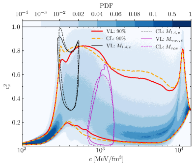
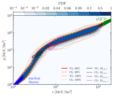
Figure 1: Left panel: PDF of the square of the sound speed shown as a function of the energy density. Red-solid (orange-dashed) lines mark the $90\%$-confidence levels of the PDF, while the solid and dashed black (purple) lines are the $90\%$ confidence levels of the PDFs relative to the centers of NSs with $M=1.4~{}M_{\odot}$ (or maximally massive, with $M=M_{\rm TOV}$) for the VL and the CL approaches, respectively. Right panel: the same as in the left panel but for the PDF of the pressure as a function of the energy density. In addition, marked by the red-dotted (orange-dotted) line is the $100\%$-confidence level for the VL (CL) method, while the uncertainties in CET (Hebeler et al., 2013) and pQCD (Fraga et al., 2014) are shown as blue and green areas, respectively.

3 Results

We next present the results of our Bayesian analyses focusing our attention on the comparison between the VL and CL approaches. In particular, we will concentrate on the EOS properties in Sec. 3.1 and on the NS properties in Sec. 3.2. The comparison will be based on contrasting the $90\%$-confidence intervals and the medians of the probability density functions (PDFs) obtained from the two analyses. For each quantity, we approximate the PDFs by counting the number of curves that cross each cell of equally spaced grids and then normalize them by the maximum count on the whole grid. Also, for readability of the figures, we only display with colormaps the PDFs for the VL analysis, referring the reader to Altiparmak et al. (2022) and to Ecker & Rezzolla (2022b) for the corresponding PDFs in the case of the CL analysis.

3.1 EOS Properties

In this section we first analyze the EOS properties that can be inferred from our two Bayesian setups. We first show in the left panel of Fig. 1 the PDFs of the sound speed that we computed using the VL approach. The PDFs show a structure very similar to the ones computed by Altiparmak et al. (2022) and Marczenko et al. (2022), that were obtained making use of the CL approach. In particular, it is possible to note that the sound speed rises rapidly till energy densities $e\approx 600~{}{\rm MeV}/{\rm fm}^{3}$, where it significantly exceeds the conformal limit $c_{\rm CFT}^{2}=1/3$. This is a well-known feature that is necessary to explain maximum-mass measurements $M\approx 2~{}M_{\odot}$ (see discussion by Bedaque & Steiner, 2015; Hoyos et al., 2016; Moustakidis et al., 2017; Kanakis-Pegios et al., 2020; Gorda et al., 2022; Brandes et al., 2022) that require a large sound speed at moderate densities, and is further enhanced if larger maximum-mass constraints are imposed, namely if $M_{\rm TOV}>2~{}M_{\odot}$ (see Ecker & Rezzolla, 2022a).

The decrease of the sound speed after the maximum at higher densities is a consequence of the perturbative-QCD constraint imposed at very large energy densities, as well as of the tidal-deformability constraint from GW170817, that disfavors stiff models with too large sound speed. Overall, when comparing the $90\%$-confidence level contours for the VL and CL approaches (red-solid and orange-dashed lines, respectively), it is apparent that not only the qualitative behavior is remarkably similar, but also the quantitative ones. These differences become more pronounced when comparing the $100\%$-confidence level contours (red-dotted and orange-dotted lines, respectively) as it is in the tails of the likelihood functions that the largest differences are imprinted in the two methods. More importantly, the statistical relevance of these stellar models is commensurate to the very low probability with which they appear.

We should note that there are also two artificial features in the PDF that are due to the parameterization method. One is the local minimum in the upper bound of the $90\%$-confidence level at $c^{2}_{s}\approx 0.7$ and $e\approx 350~{}{\rm MeV}/{\rm fm}^{3}$, which is an artifact of fixing the chemical potentials at constant values and which vanishes when sampling the chemical potentials randomly. The second one is the pronounced maximum at large densities, close to where the perturbative QCD boundary conditions are imposed. This maximum is caused by cases in which the pressure at large densities is relatively low, but where it is still possible to reach the allowed interval for $p_{\rm QCD}$ in a causal way with strongly varying sound speed slightly below $\mu=2.6\,\rm GeV$ (see also Altiparmak et al., 2022, where this is discussed in more detail).

Table 1: Neutron-star and EOS properties ($90\%$-confidence levels) from the variable likelihood (VL) and the constant likelihood (CL) methods. Listed are the radii $R$ of NSs with mass $M=1.4,2.0\,M_{\odot}$, with maximum mass $M=M_{\rm TOV}$, the corresponding tidal deformabilities $\Lambda_{1.4}$ and $\Lambda_{\rm TOV}$, as well as the number density $n_{\rm c}$, the pressure $p_{\rm c}$ and the sound speed $c^{2}_{s,c}$ at the center of typical ($M=1.4\,M_{\odot}$) and maximally massive ($M=M_{\rm TOV}$) NSs.

Method	$R_{\rm 1.4}$	$R_{\rm 2.0}$	$R_{\rm TOV}$	$\Lambda_{\rm 1.4}$	$\Lambda_{\rm TOV}$	${n_{\rm c,1.4}}$	${n_{\rm c,TOV}}$	$p_{\rm c,1.4}$	$p_{\rm c,TOV}$	$(c^{2}_{s,c})_{1.4}$	$(c^{2}_{s,c})_{\rm TOV}$
	$[{\rm km}]$	$[{\rm km}]$	$[{\rm km}]$			$[{n_{s}}]$	$[{n_{s}}]$	$[{\rm MeV}/{\rm fm}^{3}]$	$[{\rm MeV}/{\rm fm}^{3}]$
VL	$12.2_{-0.9}^{+0.9}$	$12.4_{-1.1}^{+1.0}$	$11.8_{-1.0}^{+1.3}$	$450_{-190}^{+230}$	$11_{-5}^{+18}$	$2.4_{-0.5}^{+0.7}$	$5.5_{-1.2}^{+1.2}$	$60_{-20}^{+30}$	$350_{-170}^{+210}$	$0.60_{-0.22}^{+0.23}$	$0.23_{-0.17}^{+0.38}$
CL	$12.4_{-1.0}^{+0.5}$	$12.6_{-1.4}^{+0.7}$	$12.1_{-1.3}^{+1.1}$	$490_{-220}^{+130}$	$13_{-7}^{+26}$	$2.3_{-0.4}^{+0.8}$	$5.2_{-1.1}^{+1.5}$	$50_{-10}^{+30}$	$310_{-150}^{+220}$	$0.63_{-0.25}^{+0.23}$	$0.20_{-0.16}^{+0.38}$

Also shown in the left panel of Fig. 1, respectively with solid and dashed black (purple) lines are the $90\%$ confidence levels of the PDFs relative to the centers of NSs with $M=1.4~{}M_{\odot}$ (or maximally massive, with $M=M_{\rm TOV}$) for the VL and the CL approaches, respectively. Also in this case, it is possible to note that the differences between the two evaluations of the likelihood functions are very small. More specifically, we find that in the VL (CL) approach the median value of the sound speed at the center of the NSs is $(c_{s,\,c})^{2}_{1.4}=0.60~{}(0.63)$ for the typical mass $M=1.4\,M_{\odot}$ and that $97\%$ of the EOSs have central sound speeds $c_{s,\,c}^{2}>1/3$. Similarly, we find that at the center of maximally massive NSs with $M=M_{\rm TOV}$, the sound speed are $(c_{s,\,c})^{2}_{\rm TOV}=0.23~{}(0.20)$, in agreement with the results of Ecker & Rezzolla (2022a), while only $28~{}(24)\%$ of the EOSs have central sound speeds $c_{s,\,c}^{2}>1/3$; a detailed description of the results in Fig. 1 can be found in Table 1.

In full similarity, we show in the right panel of Fig. 1 the two PDFs relative to the EOSs. Also in this case, the features of the PDF of the VL approach is very similar to that obtained previously via the CL method (Altiparmak et al., 2022). As remarked in several previous studies, a most interesting feature is the clear change of slope (also referred to as a “kink”) of the PDF at energy densities $e\approx 600~{}{\rm MeV}/{\rm fm}^{3}$. Annala et al. (2020) have interpreted this feature as a sign for the appearance of deconfinement phase transition from dense baryonic matter to quark matter (see also Motta et al. (2021) for an alternative interpretation in terms of hyperons). The $90\%$-confidence intervals of the two approaches are again shown by red-solid and orange-dashed lines and they agree remarkably well. Again, deviations can be appreciated when comparing the $100\%$-confidence intervals, marked by red and orange dotted lines, which exhibit differences at energy densities $e\approx 300~{}{\rm MeV}/{\rm fm}^{3}$. The origin of these differences is reasonably well understood. In particular, the difference in the upper bound of these contours is due to the diverse treatment of the GW constraint: the VL approach allows for larger variations than the CL method since in the latter the binary tidal deformability is assumed to be strictly $\tilde{\Lambda}<720$. As a result, the VL approach allows for EOSs that can have radii for stars $M\approx 1.4~{}M_{\odot}$ that are larger than those in the CL method (this point will be discussed also in the next section).

Finally, the right panel of Fig. 1 also reported by black (purple) solid and dashed lines the values of the pressure and energy density reached at the center of typical (maximally massive) NSs with $M=1.4~{}M_{\odot}$ ($M_{\rm TOV}$) for the VL and the CL method, respectively. Also in this case, the two sets of curves are almost identical. These contours are useful to determine the median values of the energy density and pressure at the center of representative stars. More specifically, within the VL (CL) approach we find $e_{\rm c}=390~{}(380)~{}\rm MeV/fm^{3}$ and $p_{\rm c}=60~{}(50)~{}\rm MeV/fm^{3}$ for typical mass ($M=1.4\,M_{\odot}$) NSs, while $e_{\rm c}=1100~{}(1030)~{}\rm MeV/fm^{3}$ and $p_{\rm c}=350~{}(310)~{}\rm MeV/fm^{3}$ inside maximally massive NSs ($M=M_{\rm TOV}$) (see also Table 1).

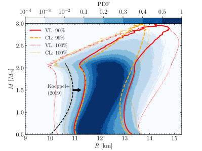
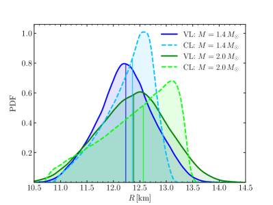
Figure 2: Left panel: the same as in the right panel of Fig. 1 but for the PDF of the stellar radius shown as a function of the stellar mass. In addition, marked by a black-dashed line is the lower bound for the radii as computed from considerations on the threshold mass (Koeppel et al., 2019). Right panel: One-dimensional PDF slices at fixed NS mass. The blue and green solid (light blue and light-green dashed) lines report the PDF cuts for the radii of a NS with $M=1.4\,M_{\odot}$ and $M=2.0\,M_{\odot}$ for the VL (CL) analysis, respectively. The vertical thin solid lines mark the corresponding median radii for the four PDFs.

3.2 Neutron-Star Properties

We next move on to the NS properties obtained from the VL and the CL approaches. As in the previous section we show for clarity only the PDFs for VL, but the confidence intervals for both VL and CL. Let us start with a discussion of the mass-radius relation shown in Fig. 2. Overall, the PDFs from the VL and CL analyses are very similar and centered around $R\approx 12\,{\rm km}$ for NSs with masses $M\lesssim 2.0\,M_{\odot}$, while they start to differ for more massive stars, where the VL approach allows for NSs with $R\sim 14\,{\rm km}$ although with rather small probability. The slightly wider PDF in the VL approach can be explained by the fact that the NICER and the GW constraints are imposed with distributions that have some support also beyond the sharp-cutoff values that are employed in the CL approach. This can be seen more clearly by comparing the outer contours ($100\%$ intervals) shown as red (VL) and orange (CL) dotted lines. As a result, the VL PDF yields upper and lower bounds for the NS radii that are less restrictive than those of the CL approach. On the other hand, when comparing the $90\%$-confidence intervals of the two approaches (solid and dashed lines) it is possible to conclude that they are essentially identical, thus underlying that the methodological differences in the use of the likelihood functions two approaches do not result in significant changes in the PDFs. Furthermore, both $90\%$-confidence levels are in good agreement with the analytic lower bound $R/{\rm km}\gtrsim 8.91+2.66\,(M/M_{\odot})-0.88\,(M/M_{\odot})^{2}$ (black-dashed line) derived when using the detection of GW170817 and the estimates on the threshold mass to prompt collapse (Koeppel et al., 2019; Tootle et al., 2021).

Also shown in the right panel of Fig. 2 are the one-dimensional PDF slices obtained in the two approaches for NSs with fixed masses $M=1.4\,M_{\odot}$ and $M=2.0\,M_{\odot}$, together with the corresponding median estimates (vertical solid lines) for their radii. These cuts show more explicitly that the VL approach results in distributions that are wider and less skewed than those for the CL case, but also that the resulting median values differ only by $\approx 200~{}{\rm m}$ (see Table 1 for details); overall, the differences between the two approaches are clearly much smaller than the current observational uncertainties.

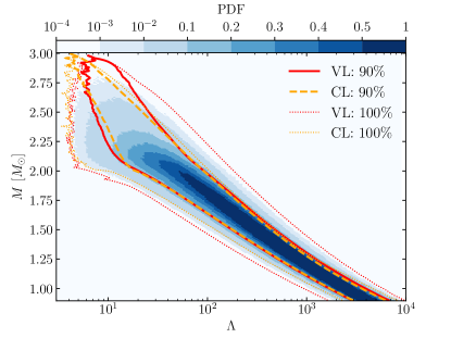
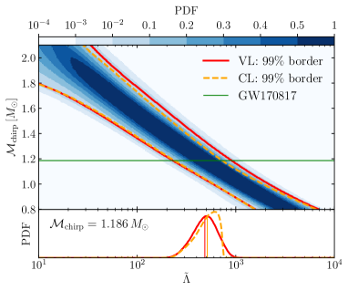
Figure 3: Left panel: PDF of the tidal deformability $\Lambda$ of isolated NSs shown as a function of the mass (the color coding is the same as that in the previous figures). Right panel: PDF of the binary tidal deformability $\tilde{\Lambda}$ of binary NS systems as a function of their chirp mass $\mathcal{M}_{\rm chirp}$. Indicated with a horizontal green line is the chirp mass of the GW170817 event, $\mathcal{M}_{\rm chirp}=1.186M_{\odot}$. The bottom part of the panel shows the corresponding one-dimensional PDF slices at $\mathcal{M}_{\rm chirp}=1.186M_{\odot}$, where the median values are marked by vertical thin lines.

We next discuss the PDFs for the tidal deformabilities of isolated and binary NSs that are plotted in Fig. 3. More specifically, in the left panel we show how the PDFs of the tidal deformability $\Lambda$ of isolated NSs depends on the gravitational mass $M$ in these two Bayesian analysis. There is a simple explanation for the overall trend of the PDF: for generic EOSs that are viable, the relative change in the NS radius is $\lesssim 6\%$ in the relevant mass range $M\approx 1-2\,M_{\odot}$, so that the tidal deformability is [see Eq. (16)] $\Lambda\sim k_{2}{M}^{-5}\sim{M}^{-p}$, with $p\gtrsim 5$. Comparing the confidence intervals of the VL and CL approaches leads to conclusions that are very similar to those drawn for the mass-radius relation in Fig. 2. More specifically, while the $100\%$ confidence interval of the VL approach is significantly wider than that of the CL method, the $90$% contours are again almost identical, so that the differences between the two methods affects mostly the less probable and therefore less important regions of the PDFs.

In the right panel of Fig. 3 we show instead the dependence of the binary tidal deformability parameter $\tilde{\Lambda}$ on the chirp mass $\mathcal{M}_{\rm chirp}$. The PDF is based on more than $9.0\times 10^{6}$ binary models with uniformly distributed mass ratios $q\in[0.4,1.0]$, i.e., a range that is reasonable according the mass ratios in binary NS systems detected so far. Analogous results from the CL approach have been shown by Altiparmak et al. (2022) and were later generalized to large-mass constraints by Ecker & Rezzolla (2022a) (see also Zhao & Lattimer, 2018, for similar studies but where no PDF is computed). Note that, in contrast to previous plots, the red-solid and orange-dashed lines show here the $99\%$-confidence levels of the PDFs. As discussed by (Ecker & Rezzolla, 2022b), these bounds – and in the particular the lower one – are of great importance to constrain the tidal deformability (and hence the EOS) using accurate measurements of the chirp mass of future GW detections of binary NS mergers. Interestingly, the lower bounds of these intervals are again almost identical, but the upper bounds differ. The reason for this is that the upper bound is directly set by the GW constraint of GW170817, while the lower bound mostly depends on the TOV constraint (Ecker & Rezzolla, 2022a).

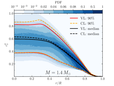
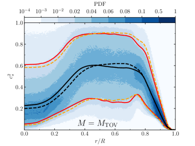
Figure 4: PDFs of the square of the sound speed as a function of normalized radial coordinate $r/R$ for NSs of mass $M=1.4\,M_{\odot}$ (left panel) and $M=M_{\rm TOV}$ (right panel). The color coding is the same as that in the previous figures, but the black-solid (black-dashed) report here the median for the VL (CL) approach.

In particular, the sharp cutoff on $\tilde{\Lambda}$ at $\mathcal{M}_{\rm chirp}=1.186\,M_{\odot}$ employed in the CL approach strongly skews the distribution towards the larger values of $\tilde{\Lambda}$. This is clearly visible in the bottom part of the right panel in Fig. 3, where we report cuts of the binary tidal deformability at $\mathcal{M}_{\rm chirp}=1.186M_{\odot}$ for the two approaches; clearly, the CL cut has a rapid fall-off for $\tilde{\Lambda}\simeq 750$, while the VL cut is almost Gaussian with a longer tail up to $\tilde{\Lambda}\simeq 1000$. As a result, the CL approach slightly underestimates the upper bound on $\tilde{\Lambda}$, while the VL approach gives a more conservative estimate. Following Altiparmak et al. (2022), we have calculated an analytic fitting function that approximate these bounds and is given by

$$\tilde{\Lambda}_{\rm min(max)}=a+b\mathcal{M}_{\rm chirp}^{c}\,,$$ (23)

where $a=-16,~{}b=560$ and $c=-5.1$ for the lower bound in both VL and CL analyses, while $a=-19~{}(0.4),~{}b=2200~{}(1900)$, and $c=-5.1~{}(-5.5)$ for the upper bound in the VL (CL) analysis.

Notwithstanding these small differences, the median values (thin vertical lines) for the case of the GW170817 event, whose chirp mass was $\mathcal{M}_{\rm chirp}=1.186M_{\odot}$, are quite similar: $\tilde{\Lambda}_{1.186}=480^{+260}_{-190}$ (VL) versus $510^{+180}_{-210}$ (CL). Furthermore, the $\tilde{\Lambda}(\mathcal{M}_{\rm chirp})$ relation can also be used the other way around. When in the future the EOS will be better constrained, it will be then possible to constrain the source-frame chirp mass. Our results can be combined with the detector frame chirp mass from the waveform matched-filter to find the redshift of the luminosity distance and thus constrain cosmological models (see, e.g.,  Messenger et al., 2014).

We next switch our attention to the PDFs of the sound speed $c_{s}^{2}(r/R)$ in the two approaches. This is presented in the left and right panels of Fig. 4, where we report the spatial dependence (i.e., as a function of the normalized radial coordinate $r/R$) of the PDFs of the sound speed inside typical ($M=1.4\,M_{\odot}$) and maximally massive ($M=M_{\rm TOV}$) NSs.

The overall behavior of the PDF for the VL approach shown here is similar to the one from the CL method presented by Ecker & Rezzolla (2022a, b). In particular, it is interesting to note that in typical NSs the sound speed rises monotonically from the surface towards the center, where it reaches values $(c^{2}_{s,\,c})_{1.4}\approx 0.6$ that are significantly larger than the conformal limit. On the other hand, in maximally massive NSs the sound speed is non-monotonic and has a local maximum with $c_{s,\rm max}^{2}>1/3$ in the outer layers (i.e., $r/R\sim 0.6$) and a local minimum at the center with $(c^{2}_{s,\,c})_{\rm TOV}\lesssim 1/3$ (see Table 1 for details). The confidence intervals and median values from VL and CL approaches are remarkably similar, even quantitatively. More specifically, for NSs with mass $M=1.4~{}M_{\odot}$ (left panel) the VL prediction for the central sound-speed, $(c^{2}_{s,\,c})_{1.4}=0.60_{-0.22}^{+0.23}$, is slightly lower than the one by CL, $(c^{2}_{s,\,c})_{1.4}=0.63_{-0.25}^{+0.23}$. Note that also in this case, the major differences are in the upper $90\%$-confidence levels, where the sharp cutoff on $\tilde{\Lambda}$ employed in the CL analysis indirectly causes a slight overestimate of the maximum possible values of the sound speed. Instead, for maximally massive NSs with $M=M_{\rm TOV}$ (right panel), an opposite behavior is observed: the central sound speed $(c^{2}_{s,\,c})_{\rm TOV}=0.23_{-0.17}^{+0.38}$, from the VL approach is slightly larger than the one from the CL method, $(c^{2}_{s,\,c})_{\rm TOV}=0.20_{-0.16}^{+0.38}$. This is due to the pQCD constraint, which introduces an anti-correlation between the sound-speed parameters at low and high densities, namely: the large values of $c_{s}^{2}$ in the low-density regions need to be compensated by lower values in the high-density region.

Finally, we show in Fig. 5 the correlation between the radius $R_{\rm TOV}$ and the central number density $n_{\rm c,TOV}$ for an NS at the maximum mass $M_{\rm TOV}$. Here again, red-solid and orange-dashed ellipses enclose the $90\%$-confidence levels obtained from the VL and the CL approach, respectively. These intervals are essentially identical, hence the relation between $R_{\rm TOV}$ and $n_{\rm c,TOV}$ is largely independent from the choice of the likelihood functions. In addition, we show results for a number of micro-physical multi-purpose EOS models of pure nuclear matter (“Nucleons”), with hyperons (“Hyperons”), with quark matter (“Quark Matter”) and models derived from holographic QCD. All EOSs are taken from the public database CompOSE (Typel et al., 2015) and correspond to beta-equilibrium slices at the lowest available temperature with electrons. Some of the corresponding properties are listed in Table 2.

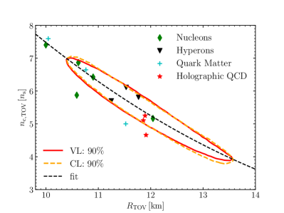
Figure 5: Relation between the normalized central number density of a maximally massive star, $n_{\rm c,TOV}/n_{s}$, and the corresponding radius, $R_{\rm TOV}$ (the color coding is the same as that in the previous figures). Also shown with various symbols are the corresponding values for EOSs of pure nuclear matter (green diamonds), with hyperons (black triangles), with quark matter (blue crosses) and models derived from holographic QCD (red stars). Shown instead with a black-dashed line is the quadratic fit given by Eq. (24).

As a concluding remark we note that the correlation between $R_{\rm TOV}$ and a normalized number density $n_{\rm c,TOV}/n_{s}$ is described by a second-order polynomial

$$\frac{n_{c,\,{\rm TOV}}}{n_{s}}=d_{0}~{}\left[1-\left(\frac{R_{\rm TOV}}{10\,\rm km}\right)\right]+d_{1}~{}\left(\frac{R_{\rm TOV}}{10\,\rm km}\right)^{2}\,,$$ (24)

where the coefficients are given by $d_{0}=27.6$ and $d_{1}=7.5$. The relative residuals are well described by a Gaussian distribution centered on zero and have a standard deviation of $3.7\%$. The importance of Eq. (24) is that it allows to estimate the maximum central density from future radius measurements of very massive NSs. We have found that a relation similar to Eq. (24) holds also when considering the radii of NSs with $M=1.4\,M_{\odot}$. In this case, the coefficients are given by $d_{0}=26.6$ and $d_{1}=7.6$, but the scatter is four times larger, reaching deviations of $\simeq 30\%$; although larger than in the case of maximally massive stars, these deviations are much smaller than the uncertainty in ${n_{c,\,{\rm TOV}}}/{n_{s}}\simeq 3.7-7.0$.

4 Conclusions

We have here investigated the systematic differences that are introduced when performing a Bayesian-inference analysis of the EOS of neutron stars employing either a variable (VL) or a constant (CL) likelihood. The former is routinely adopted in Bayesian analyses as it allows to introduce suitably variable likelihood functions for the set of constraints in the model. The latter, on the other hand, mimics the approach frequently used in those analyses where the data are used as sharp cutoffs and uniform likelihoods. The advantages of the VL method are therefore that it retains the full information on the distributions of the measurements, thus making an exhaustive usage of the data; its disadvantages are that it is more complex to implement and computationally more expensive. The advantages of the CL method, on the other hand, are to be found that the simplicity of its implementation and the comparatively smaller computational costs; its disadvantages are however that it does not fully exploit all the information from the measurements and is not adequate when the measurement results exhibit a bimodal or multi-modal behavior (a case not considered here).

In both approaches, the EOSs have been built using the sound-speed parameterization method (Annala et al., 2020; Altiparmak et al., 2022; Ecker & Rezzolla, 2022b), with identical priors for the initial EOS ensemble. For simplicity, we have restricted our comparison to observational constraints only, meaning that the prior ensembles in both cases are built by imposing the CET and perturbative QCD constraints in a fixed-cutoff manner. As a result, the likelihood functions of the CET and perturbative QCD constraints are constant, while that of the observational constraints are suitably variable. Overall, the statistics are performed making use of more than $1.5\times 10^{5}$ causal and thermodynamically consistent posterior EOSs that satisfy the nuclear theory and perturbative QCD boundary conditions, as well as the observational constraints from pulsars and GW measurements.

In our analysis we have considered how the two inferences differ when considering either the properties of the EOS (e.g., sound speed, pressure behavior as a function of the energy density, and sound-speed variation within the stellar interior) or of the NSs (masses, radii, and tidal deformabilities). In all cases, we have found that the two approaches lead to very similar results and that the $90\%$-confidence levels are essentially overlapping. Some differences do appear when comparing the $100\%$-confidence levels, but these differences concern regions of the PDFs where the probability is extremely small, thus leading to the conclusion that the role played by the functional form of the likelihood function in our Bayesian inference is small.

When concentrating on what are the main sources of difference we note that these can almost always be attributed to the sharp cutoff on $\tilde{\Lambda}$ (i.e., $\tilde{\Lambda}\leq 720$) employed in the CL analysis, which indirectly causes a slight overestimate of the maximum possible values of the sound speed in a range of energy densities inside that allowed for plausible stellar models, but also a slight underestimate of the maximum possible values of the stellar radii for all masses. Finally, the sharp cutoff on ${\tilde{\Lambda}}$ also leads to a smaller upper bound on $\tilde{\Lambda}$ with a consequent underestimate of the binary tidal deformability using measured chirp mass.

In addition to the comparison between the two inference approaches and the assessment of the role of the likelihood functions, our analysis has also produced two noteworthy results. Firstly, a clear inverse correlation between the normalized central number density of a maximally massive star, $n_{\rm c,TOV}/n_{s}$, and the radius of either a typical $M=1.4\,M_{\odot}$ NS or of the corresponding maximally massive star, $R_{\rm TOV}$. Once a reliable measurement of one of these radii is accomplished, the relation will provide a rather stringent estimate of the number density that needs to be matched by studies building EOSs from nuclear theory. Secondly, and most importantly, it has confirmed the relation found between the chirp mass $\mathcal{M}_{\rm chirp}$ and the binary tidal deformability $\tilde{\Lambda}$. We need to underline that the importance of this result is that it relates a quantity that is directly measurable – and is very accurately measured – from gravitational-wave observations, $\mathcal{M}_{\rm chirp}$, with a quantity that contains important information on the micro-physics $\tilde{\Lambda}$. For example, when considering the case of the GW170817 event, whose chirp mass is $\mathcal{M}_{\rm chirp}=1.186M_{\odot}$, the bounds obtained in the case of the VL approach are $\tilde{\Lambda}_{1.186}=480^{+260}_{-190}$.

Appendix A Comparison to HESS J1731-347

As mentioned in the main text, Doroshenko et al. (2022) have recently reported the combined mass-radius measurement of a very light compact object within the supernova remnant HESS J1731-347 having a mass $M=0.77^{+0.20}_{-0.17}~{}M_{\odot}$ and radius $R=10.4^{+0.86}_{-0.78}~{}\,{\rm km}$. Because of the untypically small values of mass and radius, that were deduced from combining distance estimates from Gaia observations with X-ray spectrum modelling, the nature and composition of this object is currently unclear. Indeed, the compact star is speculated to be either the lightest (and smallest) NS known or a “strange star” composed of more exotic constituents than just nucleonic matter.

Assuming that HESS J1731-347 is composed of standard nuclear matter and maintaining the same uncertainties in the mass measurement as those reported by Doroshenko et al. (2022), we can use the results of our Bayesian analysis with VL to infer the distribution of stellar radii compatible with our posterior PDFs. In particular, we show in the left panel of Fig. 6 the $68.3\%$ and $95.4\%$ confidence levels of the PDFs for the mass and radius of NSs as obtained in our analysis (thick and thin red solid lines, respectively) together with the corresponding levels provided by Doroshenko et al. (2022) (thick and thin light-blue solid lines, respectively) obtained from the fitting of the X-ray data alone using a single-temperature carbon atmosphere model and Gaia parallax priors. Already a crude comparison reveals that our analysis tends to predict systematically larger radii within the mass of interest, with a difference of about one kilometer. It is a matter of concern that a good portion of the allowed space for the mass and radius suggested by Doroshenko et al. (2022) violates the lower-limits on the radius set by threshold mass by Koeppel et al. (2019) (see also the estimate of Bauswein et al., 2017, which requires $R_{1.6}\geq 10.30\,{\rm km}$), although it is fair to recognise that such lower limits have been deduced for larger masses.

Our tendency to have larger radii can be seen more clearly in the right panel of Fig. 6, where we compare the corresponding one-dimensional PDF slices at $M=0.77~{}M_{\odot}$ from the analysis of Doroshenko et al. (2022) (light-blue solid line) and from our inference (red solid line). Clearly, the corresponding median values can be seen to differ by $\approx 1.5~{}\,{\rm km}$. Combining the two PDF slices and properly normalizing leads to PDF shown with the blue dashed line, which suggests a radius $R=11.43^{+0.64}_{-0.60}~{}\,{\rm km}$ in $90\%$ interval and therefore about one kilometer larger than that deduced by Doroshenko et al. (2022). It will be interesting to see if this difference persists when the present (crude) comparison is further refined by imposing in our Bayesian analysis the constraints coming from the measurements of Doroshenko et al. (2022) and by lower limits set by Koeppel et al. (2019); we postpone this investigation to future work.

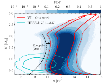
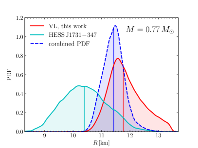
Figure 6: Left panel: Comparison of the mass-radius data for HESS J1731-347 and the mass-radius distribution of our VL analysis. Thin (thick) red lines represent the $95.4\%$ ($68.3\%$) confidence level, while light-blue contours mark the $95.4\%$ ($68.3\%$) measurement posterior samples of HESS J1731-347. Right panel: One-dimensional PDF slices at constant mass $M=0.77\,M_{\odot}$ using the same color convention as in the left panel. The blue-dashed line combines the two PDFs and provides our new estimate for the radius of HESS J1731-347.

Appendix B EOSs employed in Figure 5

For completeness, we provide here the basic properties of the EOSs used as symbols in Fig. 5. These properties are listed in Table 2 and we provide information on the NS radii ($R_{\rm 1.4},~{}R_{\rm 2.0}$ at $M=1.4,~{}2.0~{}M_{\odot}$ and ${R_{\rm TOV}}$ at $M=M_{\rm TOV}$), on the maximum mass $M_{\rm TOV}$ and on the binary tidal deformability $\tilde{\Lambda}_{1.186}$ of GW170817-like binaries with chirp mass $\mathcal{M}_{c}=1.186~{}M_{\odot}$ when considering two different mass ratios, i.e., $q=1,0.7$.

Table 2: Properties of the EOS models used in Fig. 5. The properties listed are the corresponding NS radii $R_{\rm 1.4},~{}R_{\rm 2.0}$ and ${R_{\rm TOV}}$ at $M=1.4,~{}2.0~{}M_{\odot}$ and the maximum mass $M_{\rm TOV}$, respectively, as well as the binary tidal deformability parameter $\tilde{\Lambda}_{1.186}$ of GW170817 like binaries with chirp mass $\mathcal{M}_{c}=1.186~{}M_{\odot}$ for two different mass ratios $q=1,0.7$.

Type	EOS	${R_{\rm 1.4}}$	${R_{\rm 2.0}}$	${R_{\rm TOV}}$	${M_{\rm TOV}}$	$\tilde{\Lambda}^{\rm q=1~{}(0.7)}_{1.186}$	Ref.
		$[{\rm km}]$	$[{\rm km}]$	$[{\rm km}]$	$[{M_{\odot}}]$
Nucleons	DD2	$13.76$	$13.45$	$12.04$	$2.42$	$816~{}(784)$	Hempel & Schaffner-Bielich (2010)
	LS220	$12.66$	$11.34$	$10.62$	$2.04$	$574~{}(569)$	Schneider et al. (2017)
	SFHx	$12.4$	$11.78$	$10.9$	$2.13$	$464~{}(451)$	Steiner et al. (2013)
	SLy4	$11.73$	$10.67$	$10.0$	$2.05$	$313~{}(309)$	Schneider et al. (2017)
	KOST2	$11.58$	$11.21$	$10.2$	$2.22$	$358~{}(352)$	Togashi et al. (2017)
Hyperons	DD2$\Lambda\phi$	$13.75$	$12.84$	$11.77$	$2.1$	$813~{}(772)$	Banik et al. (2014)
	DD2Y	$13.75$	$12.33$	$11.53$	$2.04$	$814~{}(767)$	Marques et al. (2017)
	DD2Y$\Delta$ 1.1-1.1	$13.47$	$12.22$	$10.63$	$2.17$	$698~{}(687)$	Raduta et al. (2020)
Quark Matter	RDF1.6	$12.46$	$10.31$	$10.04$	$2.01$	$509~{}(501)$	Bastian (2021)
	RDF1.7	$12.46$	$11.44$	$10.76$	$2.11$	$508~{}(506)$	Bastian (2021)
	TM1B145	$12.92$	$12.25$	$10.57$	$2.27$	$625~{}(612)$	Sagert et al. (2010)
	V-QCD soft	$12.42$	$12.01$	$11.91$	$2.02$	$537~{}(517)$	Demircik et al. (2021)
	V-QCD interm	$12.51$	$12.4$	$11.86$	$2.14$	$565~{}(543)$	Demircik et al. (2021)
	V-QCD stiff	$12.65$	$12.85$	$11.89$	$2.34$	$617~{}(591)$	Demircik et al. (2021)

References

- Abbott et al. (2018) Abbott, B. P., Abbott, R., Abbott, T. D., et al. 2018, Physical Review Letters, 121, 161101, doi: 10.1103/PhysRevLett.121.161101
- Abbott et al. (2020) —. 2020, Classical and Quantum Gravity, 37, 055002, doi: 10.1088/1361-6382/ab685e
- Al-Mamun et al. (2021) Al-Mamun, M., Steiner, A. W., Nättilä, J., et al. 2021, Phys. Rev. Lett., 126, 061101, doi: 10.1103/PhysRevLett.126.061101
- Altiparmak et al. (2022) Altiparmak, S., Ecker, C., & Rezzolla, L. 2022, ApJL, in press, arXiv:2203.14974. https://arxiv.org/abs/2203.14974
- Annala et al. (2022) Annala, E., Gorda, T., Katerini, E., et al. 2022, Physical Review X, 12, 011058, doi: 10.1103/PhysRevX.12.011058
- Annala et al. (2020) Annala, E., Gorda, T., Kurkela, A., Nättilä, J., & Vuorinen, A. 2020, Nature Physics, 16, 907, doi: 10.1038/s41567-020-0914-9
- Antoniadis et al. (2013) Antoniadis, J., Freire, P. C. C., Wex, N., et al. 2013, Science, 340, 448, doi: 10.1126/science.1233232
- Arzoumanian et al. (2018) Arzoumanian, Z., Brazier, A., Burke-Spolaor, S., et al. 2018, Astrophys. J., Supp., 235, 37, doi: 10.3847/1538-4365/aab5b0
- Ashton et al. (2019) Ashton, G., Hübner, M., Lasky, P. D., et al. 2019, Bilby: Bayesian inference library. http://ascl.net/1901.011
- Banik et al. (2014) Banik, S., Hempel, M., & Bandyopadhyay, D. 2014, Astrohys. J. Suppl., 214, 22, doi: 10.1088/0067-0049/214/2/22
- Bastian (2021) Bastian, N.-U. F. 2021, Phys. Rev. D, 103, 023001, doi: 10.1103/PhysRevD.103.023001
- Bauswein et al. (2017) Bauswein, A., Just, O., Janka, H.-T., & Stergioulas, N. 2017, Astrophys. J. Lett., 850, L34, doi: 10.3847/2041-8213/aa9994
- Baym et al. (1971) Baym, G., Pethick, C., & Sutherland, P. 1971, Astrophys. J., 170, 299, doi: 10.1086/151216
- Bedaque & Steiner (2015) Bedaque, P., & Steiner, A. W. 2015, Physical Review Letters, 114, 031103, doi: 10.1103/PhysRevLett.114.031103
- Beloin et al. (2019) Beloin, S., Han, S., Steiner, A. W., & Odbadrakh, K. 2019, Phys. Rev. C, 100, 055801, doi: 10.1103/PhysRevC.100.055801
- Bose et al. (2018) Bose, S., Chakravarti, K., Rezzolla, L., Sathyaprakash, B. S., & Takami, K. 2018, Phys. Rev. Lett., 120, 031102, doi: 10.1103/PhysRevLett.120.031102
- Brandes et al. (2022) Brandes, L., Weise, W., & Kaiser, N. 2022. https://arxiv.org/abs/2208.03026
- Buchner (2016) Buchner, J. 2016, PyMultiNest: Python interface for MultiNest. http://ascl.net/1606.005
- Demircik et al. (2021) Demircik, T., Ecker, C., & Järvinen, M. 2021, arXiv e-prints, arXiv:2112.12157. https://arxiv.org/abs/2112.12157
- Dexheimer et al. (2019) Dexheimer, V., Constantinou, C., Most, E. R., et al. 2019, Universe, 5, 129, doi: 10.3390/universe5050129
- Dietrich et al. (2020) Dietrich, T., Coughlin, M. W., Pang, P. T. H., et al. 2020, Science, 370, 1450, doi: 10.1126/science.abb4317
- Doroshenko et al. (2022) Doroshenko, V., Suleimanov, V., Pühlhofer, G., & Santangelo, A. 2022, Nature Astronomy, 1, doi: 10.1038/s41550-022-01800-1
- Drischler et al. (2020) Drischler, C., Melendez, J. A., Furnstahl, R. J., & Phillips, D. R. 2020, Phys. Rev. C, 102, 054315, doi: 10.1103/PhysRevC.102.054315
- Ecker & Rezzolla (2022) Ecker, C., & Rezzolla, L. 2022, ApJL, in press, arXiv:2207.04417. https://arxiv.org/abs/2207.04417
- Ecker & Rezzolla (2022a) Ecker, C., & Rezzolla, L. 2022a. https://arxiv.org/abs/2209.08101
- Ecker & Rezzolla (2022b) —. 2022b. https://arxiv.org/abs/2207.04417
- Ferreira & Providência (2021) Ferreira, M., & Providência, C. 2021, J. Cosmology Astropart. Phys, 2021, 011, doi: 10.1088/1475-7516/2021/07/011
- Fonseca et al. (2021) Fonseca, E., Cromartie, H. T., Pennucci, T. T., et al. 2021, Astrophys. J. Lett., 915, L12, doi: 10.3847/2041-8213/ac03b8
- Fraga et al. (2014) Fraga, E. S., Kurkela, A., & Vuorinen, A. 2014, Astrophys. J. Lett., 781, L25, doi: 10.1088/2041-8205/781/2/L25
- Freedman & McLerran (1977) Freedman, B. A., & McLerran, L. D. 1977, Phys. Rev. D, 16, 1169, doi: 10.1103/PhysRevD.16.1169
- Fujimoto et al. (2021) Fujimoto, Y., Fukushima, K., & Murase, K. 2021, arXiv e-prints, arXiv:2101.08156. https://arxiv.org/abs/2101.08156
- Gandolfi et al. (2019) Gandolfi, S., Lippuner, J., Steiner, A. W., et al. 2019, arXiv e-prints, arXiv:1903.06730. https://arxiv.org/abs/1903.06730
- Gorda et al. (2022) Gorda, T., Komoltsev, O., & Kurkela, A. 2022. https://arxiv.org/abs/2204.11877
- Gorda et al. (2022) Gorda, T., Komoltsev, O., & Kurkela, A. 2022, arXiv e-prints, arXiv:2204.11877. https://arxiv.org/abs/2204.11877
- Gorda et al. (2021a) Gorda, T., Kurkela, A., Paatelainen, R., Säppi, S., & Vuorinen, A. 2021a, Phys. Rev. D, 104, 074015, doi: 10.1103/PhysRevD.104.074015
- Gorda et al. (2021b) —. 2021b, Phys. Rev. Lett., 127, 162003, doi: 10.1103/PhysRevLett.127.162003
- Greif et al. (2019) Greif, S. K., Raaijmakers, G., Hebeler, K., Schwenk, A., & Watts, A. L. 2019, Mon. Not. R. Astron. Soc., 485, 5363, doi: 10.1093/mnras/stz654
- Han et al. (2022a) Han, M.-Z., Huang, Y.-J., Tang, S.-P., & Fan, Y.-Z. 2022a, arXiv e-prints, arXiv:2207.13613. https://arxiv.org/abs/2207.13613
- Han et al. (2021) Han, M.-Z., Jiang, J.-L., Tang, S.-P., & Fan, Y.-Z. 2021, ApJ, 919, 11, doi: 10.3847/1538-4357/ac11f8
- Han et al. (2022b) Han, M.-Z., Tang, S.-P., & Fan, Y.-Z. 2022b, arXiv e-prints, arXiv:2205.03855. https://arxiv.org/abs/2205.03855
- Hebeler et al. (2013) Hebeler, K., Lattimer, J. M., Pethick, C. J., & Schwenk, A. 2013, Astrophys. J., 773, 11, doi: 10.1088/0004-637X/773/1/11
- Hebeler et al. (2013) Hebeler, K., Lattimer, J. M., Pethick, C. J., & Schwenk, A. 2013, Astrophys. J., 773, 11, doi: 10.1088/0004-637X/773/1/11
- Hempel & Schaffner-Bielich (2010) Hempel, M., & Schaffner-Bielich, J. 2010, Nucl. Phys., A837, 210, doi: 10.1016/j.nuclphysa.2010.02.010
- Hernandez Vivanco et al. (2020) Hernandez Vivanco, F., Smith, R., Thrane, E., & Lasky, P. D. 2020, MNRAS, 499, 5972, doi: 10.1093/mnras/staa3243
- Hoyos et al. (2016) Hoyos, C., Jokela, N., Rodríguez Fernández, D., & Vuorinen, A. 2016, Phys. Rev. D, 94, 106008, doi: 10.1103/PhysRevD.94.106008
- Huth et al. (2021) Huth, S., et al. 2021. https://arxiv.org/abs/2107.06229
- Ivanytskyi & Blaschke (2022) Ivanytskyi, O., & Blaschke, D. 2022, Eur. Phys. J. A, 58, 152, doi: 10.1140/epja/s10050-022-00808-5
- Jiang et al. (2020) Jiang, J.-L., Tang, S.-P., Wang, Y.-Z., Fan, Y.-Z., & Wei, D.-M. 2020, ApJ, 892, 55, doi: 10.3847/1538-4357/ab77cf
- Jie Li et al. (2021) Jie Li, J., Sedrakian, A., & Alford, M. 2021, arXiv e-prints, arXiv:2108.13071. https://arxiv.org/abs/2108.13071
- Kanakis-Pegios et al. (2020) Kanakis-Pegios, A., Koliogiannis, P. S., & Moustakidis, C. C. 2020, Phys. Rev. C, 102, 055801, doi: 10.1103/PhysRevC.102.055801
- Keller et al. (2021) Keller, J., Wellenhofer, C., Hebeler, K., & Schwenk, A. 2021, Phys. Rev. C, 103, 055806, doi: 10.1103/PhysRevC.103.055806
- Koeppel et al. (2019) Koeppel, S., Bovard, L., & Rezzolla, L. 2019, Astrophys. J. Lett., 872, L16, doi: 10.3847/2041-8213/ab0210
- Komoltsev & Kurkela (2022) Komoltsev, O., & Kurkela, A. 2022, Phys. Rev. Lett., 128, 202701, doi: 10.1103/PhysRevLett.128.202701
- Landry & Essick (2019) Landry, P., & Essick, R. 2019, Phys. Rev. D, 99, 084049, doi: 10.1103/PhysRevD.99.084049
- Legred et al. (2022) Legred, I., Chatziioannou, K., Essick, R., & Landry, P. 2022, Phys. Rev. D, 105, 043016, doi: 10.1103/PhysRevD.105.043016
- Linares et al. (2018) Linares, M., Shahbaz, T., & Casares, J. 2018, ApJ, 859, 54, doi: 10.3847/1538-4357/aabde6
- Lindblom (2010) Lindblom, L. 2010, Phys. Rev. D, 82, 103011, doi: 10.1103/PhysRevD.82.103011
- Lindblom (2018) —. 2018, Phys. Rev. D, 97, 123019, doi: 10.1103/PhysRevD.97.123019
- Marczenko et al. (2022) Marczenko, M., McLerran, L., Redlich, K., & Sasaki, C. 2022, arXiv e-prints, arXiv:2207.13059. https://arxiv.org/abs/2207.13059
- Margalit & Metzger (2017) Margalit, B., & Metzger, B. D. 2017, Astrophys. J. Lett., 850, L19, doi: 10.3847/2041-8213/aa991c
- Marques et al. (2017) Marques, M., Oertel, M., Hempel, M., & Novak, J. 2017, Phys. Rev. C, 96, 045806, doi: 10.1103/PhysRevC.96.045806
- Messenger et al. (2014) Messenger, C., Takami, K., Gossan, S., Rezzolla, L., & Sathyaprakash, B. S. 2014, Physical Review X, 4, 041004, doi: 10.1103/PhysRevX.4.041004
- Miller et al. (2019) Miller, M. C., Lamb, F. K., Dittmann, A. J., et al. 2019, Astrophys. J. Lett., 887, L24, doi: 10.3847/2041-8213/ab50c5
- Miller et al. (2021) —. 2021, Astrophys. J. Lett., 918, L28, doi: 10.3847/2041-8213/ac089b
- Morawski & Bejger (2020) Morawski, F., & Bejger, M. 2020, A&A, 642, A78, doi: 10.1051/0004-6361/202038130
- Most et al. (2020) Most, E. R., Weih, L. R., & Rezzolla, L. 2020, Mon. Not. R. Astron. Soc., 496, L16, doi: 10.1093/mnrasl/slaa079
- Most et al. (2018) Most, E. R., Weih, L. R., Rezzolla, L., & Schaffner-Bielich, J. 2018, Phys. Rev. Lett., 120, 261103, doi: 10.1103/PhysRevLett.120.261103
- Motta et al. (2021) Motta, T. F., Guichon, P. A. M., & Thomas, A. W. 2021, Nucl. Phys. A, 1009, 122157, doi: 10.1016/j.nuclphysa.2021.122157
- Moustakidis et al. (2017) Moustakidis, C. C., Gaitanos, T., Margaritis, C., & Lalazissis, G. A. 2017, Physical Review C, 95, 045801, doi: 10.1103/PhysRevC.95.045801
- Nathanail et al. (2021) Nathanail, A., Most, E. R., & Rezzolla, L. 2021, Astrophys. J. Lett., 908, L28, doi: 10.3847/2041-8213/abdfc6
- O’Boyle et al. (2020) O’Boyle, M. F., Markakis, C., Stergioulas, N., & Read, J. S. 2020, Phys. Rev. D, 102, 083027, doi: 10.1103/PhysRevD.102.083027
- Raaijmakers et al. (2021) Raaijmakers, G., Greif, S. K., Hebeler, K., et al. 2021, Astrophys. J. Lett., 918, L29, doi: 10.3847/2041-8213/ac089a
- Raduta et al. (2020) Raduta, A. R., Oertel, M., & Sedrakian, A. 2020, MNRAS, 499, 914, doi: 10.1093/mnras/staa2491
- Read et al. (2009) Read, J. S., Lackey, B. D., Owen, B. J., & Friedman, J. L. 2009, Phys. Rev. D, 79, 124032, doi: 10.1103/PhysRevD.79.124032
- Rezzolla et al. (2018) Rezzolla, L., Most, E. R., & Weih, L. R. 2018, Astrophys. J. Lett., 852, L25, doi: 10.3847/2041-8213/aaa401
- Rezzolla & Zanotti (2013) Rezzolla, L., & Zanotti, O. 2013, Relativistic Hydrodynamics (Oxford, UK: Oxford University Press), doi: 10.1093/acprof:oso/9780198528906.001.0001
- Riley et al. (2019) Riley, T. E., Watts, A. L., Bogdanov, S., et al. 2019, Astrophys. J. Lett., 887, L21, doi: 10.3847/2041-8213/ab481c
- Riley et al. (2021) Riley, T. E., Watts, A. L., Ray, P. S., et al. 2021, Astrophys. J. Lett., 918, L27, doi: 10.3847/2041-8213/ac0a81
- Romani et al. (2022) Romani, R. W., Kandel, D., Filippenko, A. V., Brink, T. G., & Zheng, W. 2022, Astrophys. J. Lett., 934, L18, doi: 10.3847/2041-8213/ac8007
- Ruiz et al. (2018) Ruiz, M., Shapiro, S. L., & Tsokaros, A. 2018, Phys. Rev. D, 97, 021501, doi: 10.1103/PhysRevD.97.021501
- Sagert et al. (2010) Sagert, I., Fischer, T., Hempel, M., et al. 2010, Journal of Physics G Nuclear Physics, 37, 094064, doi: 10.1088/0954-3899/37/9/094064
- Schneider et al. (2017) Schneider, A. S., Roberts, L. F., & Ott, C. D. 2017, Phys. Rev. C, 96, 065802, doi: 10.1103/PhysRevC.96.065802
- Scott (1992) Scott, D. 1992, Multivariate Density Estimation: Theory, Practice and Visualization (New York, USA: John Wiley & Sons, Inc.), doi: 10.1002/9780470316849
- Shibata et al. (2019) Shibata, M., Zhou, E., Kiuchi, K., & Fujibayashi, S. 2019, Phys. Rev. D, 100, 023015, doi: 10.1103/PhysRevD.100.023015
- Soma et al. (2022) Soma, S., Wang, L., Shi, S., Stöcker, H., & Zhou, K. 2022, arXiv e-prints, arXiv:2209.08883. https://arxiv.org/abs/2209.08883
- Somasundaram et al. (2022) Somasundaram, R., Tews, I., & Margueron, J. 2022, arXiv e-prints, arXiv:2204.14039. https://arxiv.org/abs/2204.14039
- Steiner et al. (2013) Steiner, A. W., Hempel, M., & Fischer, T. 2013, Astrophys. J., 774, 17, doi: 10.1088/0004-637X/774/1/17
- Tang et al. (2021) Tang, S.-P., Jiang, J.-L., Han, M.-Z., Fan, Y.-Z., & Wei, D.-M. 2021, Phys. Rev. D, 104, 063032, doi: 10.1103/PhysRevD.104.063032
- The LIGO Scientific Collaboration & The Virgo Collaboration (2017) The LIGO Scientific Collaboration, & The Virgo Collaboration. 2017, Phys. Rev. Lett., 119, 161101, doi: 10.1103/PhysRevLett.119.161101
- The LIGO Scientific Collaboration et al. (2019) The LIGO Scientific Collaboration, the Virgo Collaboration, Abbott, B. P., et al. 2019, Physical Review X, 9, 011001, doi: 10.1103/PhysRevX.9.011001
- Togashi et al. (2017) Togashi, H., Nakazato, K., Takehara, Y., et al. 2017, Nucl. Phys., A961, 78, doi: 10.1016/j.nuclphysa.2017.02.010
- Tootle et al. (2021) Tootle, S. D., Papenfort, L. J., Most, E. R., & Rezzolla, L. 2021, Astrophys. J. Lett., 922, L19, doi: 10.3847/2041-8213/ac350d
- Traversi et al. (2020) Traversi, S., Char, P., & Pagliara, G. 2020, ApJ, 897, 165, doi: 10.3847/1538-4357/ab99c1
- Typel et al. (2015) Typel, S., Oertel, M., & Klähn, T. 2015, Physics of Particles and Nuclei, 46, 633, doi: 10.1134/S1063779615040061
- Vuorinen (2003) Vuorinen, A. 2003, Phys. Rev. D, 68, 054017, doi: 10.1103/PhysRevD.68.054017
- Zhao & Lattimer (2018) Zhao, T., & Lattimer, J. M. 2018, Phys. Rev. D, 98, 063020, doi: 10.1103/PhysRevD.98.063020