P3H–22–102, TTP22–061, KEK–TH–2468

Chasing the two-Higgs doublet model
in the di-Higgs production

Syuhei Iguro,${}^{{\includegraphics[height=6.72003pt]{logo/TTP_logo.pdf}},{\includegraphics[height=6.72003pt]{logo/IAP.pdf}}}$ Teppei Kitahara,${}^{{\includegraphics[height=6.72003pt]{logo/IAR_logo.pdf}},{\includegraphics[height=6.72003pt]{logo/KMI_logo.pdf}},{\includegraphics[height=6.72003pt]{logo/KEK_logo.pdf}},{\includegraphics[height=6.72003pt]{logo/ITP_logo.pdf}}}$ Yuji Omura,${}^{{\includegraphics[height=6.72003pt]{logo/kindai_logo.pdf}}}$
and Hantian Zhang${}^{{\includegraphics[height=6.72003pt]{logo/TTP_logo.pdf}}}$

	Institute for Theoretical Particle Physics (TTP), Karlsruhe Institute of Technology (KIT),
	Engesserstraße 7, 76131 Karlsruhe, Germany
	Institute for Astroparticle Physics (IAP), KIT, Hermann-von-Helmholtz-Platz 1,
	76344 Eggenstein-Leopoldshafen, Germany
	Institute for Advanced Research, Nagoya University, Nagoya 464–8601, Japan
	Kobayashi-Maskawa Institute for the Origin of Particles and the Universe,
	Nagoya University, Nagoya 464–8602, Japan
	KEK Theory Center, IPNS, KEK, Tsukuba 305–0801, Japan
	CAS Key Laboratory of Theoretical Physics, Institute of Theoretical Physics,
	Chinese Academy of Sciences, Beijing 100190, China
	Department of Physics, Kindai University, Higashi-Osaka, Osaka 577–8502, Japan
	E-mail: igurosyuhei@gmail.com, teppeik@kmi.nagoya-u.ac.jp,
yomura@phys.kindai.ac.jp, hantian.zhang@kit.edu

We investigate the di-Higgs production at the Large Hadron Collider in the two-Higgs doublet model (2HDM). In particular, we study the production of an extra neutral Higgs boson $\phi$ in association with the Standard Model (SM) Higgs boson $h$ in the Higgs alignment limit. We analyze two scenarios where the additional Higgs $\phi$ is CP-even or -odd state with a large top-Yukawa interaction. The leading contribution of this production comes from the top-quark loop-induced gluon-fusion channel $gg\to h\phi$. The measurement of the $h\phi$ production can probe the quartic couplings in the Higgs potential as well as the top-Yukawa couplings. Imposing both theoretical constraints (from the perturbative unitarity and the vacuum stability bounds) and experimental bounds (from the SM Higgs and flavor physics measurements) on the 2HDM parameter space, we calculate the production cross-section of $gg\to h\phi$. Furthermore, we scrutinize these processes in the parameter spaces where the CMS di-tau and di-photon excesses around 100 GeV, and/or the muon $g-2$ anomaly can be accommodated.

Keywords: Multi-Higgs Models, Di-Higgs Production, Large Hadron Collider

 

 

1 Introduction

The spontaneous symmetry breaking of $SU(2)_{L}\times U(1)_{Y}$ is caused by a Higgs field in the Standard Model (SM) [1, 2], where the Higgs potential is given by a negative mass squared term and a quartic coupling, and the Higgs obtains non-vanishing vacuum expectation value (VEV). Through the couplings between the Higgs and the other SM fields, fermions obtain their masses and the $SU(2)_{L}$ gauge bosons acquire the masses by absorbing the Nambu–Goldstone (NG) bosons [3, 4, 5]. This picture is very successful in explaining experimental results; however, the origin of the negative mass squared term is unknown. Therefore it motivates the further understanding of the Higgs sector. There may be multiple Higgs fields and the scalar potential may be more complicated than the one in the SM.

One promising way to reveal the vacuum structure given by the scalar potential is to test signals involving (extra) scalars in the final state at the Large Hadron Collider (LHC). The Higgs boson pair production, for instance, gives information about the triple-Higgs coupling [6, 7]. Precise calculations of the dominant contribution $gg\to hh$ within the SM have been performed at next-to-leading order (NLO) QCD accuracy [8, 9, 10, 11, 12, 13, 14, 15, 16, 17, 18]. Its frontier has been pushing up to next-to-next-to-next-to-leading order (N³LO) QCD [19, 20, 21, 22, 23, 24, 25, 26, 27, 28, 29] and NLO electroweak (EW) [30, 31, 32] in various approximations. Currently, it has been still difficult to test the scalar potential parameters directly at the LHC due to the small Higgs-pair production cross section compared to the huge QCD background [33, 34]. Nevertheless, thanks to the accumulating luminosity at the LHC and improvements in the flavor-tagging algorithm [35, 36], the measurement of the Higgs-pair production has provided profound information on the triple-Higgs coupling and thus the shape of the Higgs potential [37, 38, 39, 40, 41, 42, 43, 44, 45, 46, 47, 48]. The future prospects are discussed in Refs. [7, 49].

Multi-Higgs doublet models often appear as low-energy effective field theories: the supersymmetric standard model [50, 51], left-right symmetric model [52], and so on. Therefore, it is interesting to investigate the new physics models with extra Higgs doublets. After the SM Higgs discovery in 2012 [53, 54], it has turned out that its interactions are well consistent with the SM predictions within the current experimental and theoretical uncertainties [55, 56]. This fact may imply that the additional scalars live in the considerably high energy region which leads to the decoupling feature, or they are hidden from the measurements by the Higgs alignment feature where the additional Higgs doublets do not mix with the SM-like Higgs doublet. In this paper, we pursue the latter possibility, and propose a novel way to probe a relatively light neutral scalar through the di-Higgs production channel at the LHC.

We consider the two-Higgs doublet model (2HDM) as a working example of new physics, and assume the existence of a light additional neutral Higgs boson. There are many motivations for the light additional scalar. For example, it is known that the CP violation of the SM, namely the complex phase of the CKM matrix, is not large enough to generate the observed baryon asymmetry of the Universe (BAU) [57]. In addition, the observed 125 GeV Higgs mass is too heavy for the strong first-order phase transition (SFOPT), which is required for a viable explanation of the BAU. For a successful SFOPT, the modification of the SM Higgs potential is necessary and hence extensions of the Higgs sector are well motivated [58, 59, 60, 61]. It is shown that an additional scalar with $\mathcal{O}(1)$ top-Yukawa coupling can provide the large CP violation and explain the observed BAU [62]. A joint explanation of the BAU and the radiative neutrino mass with light scalars is also discussed [63, 64, 65].

Moreover, a light (pseudo) scalar would explain the discrepancy in the muon anomalous magnetic moment (muon $g-2$) [66, 67, 68, 69], whose SM expectation value is based on the $e^{+}e^{-}\to$ hadrons data. Note that the recent evaluations of a window observable for the hadronic vacuum polarization based on lattice QCD simulation [70] are shown in Refs. [71, 72, 73, 74, 75, 76], and a large discrepancy with the $e^{+}e^{-}\to\pi^{+}\pi^{-}$ data has been reported in Refs. [77, 78, 79]. In the flavor-conserving 2HDM where only flavor-diagonal Yukawa interactions are introduced, an additional light scalar could explain the muon $g-2$ anomaly via the two-loop Barr-Zee diagram [80]. Here, note that a large mass gap between the lightest neutral scalar and the charged scalar is necessary to avoid collider constraints.

In recent years, not significant enough but mild excesses around 95 GeV have been reported in $\tau\bar{\tau}$[81] and $\gamma\gamma$ [82] resonance searches by the CMS collaboration, and in $b\bar{b}$ mode by the LEP experiment [83]. In Ref. [84], it is shown that an additional CP-odd pseudo-scalar $\phi$ with a large $\phi\bar{t}\gamma_{5}{t}$ interaction can still provide a viable solution to the $\tau\bar{\tau}$ excess reported by the CMS, while the CP-even scalar explanation is shown to be difficult. In the light CP-odd scalar scenario, the production cross-section of $pp\to t\bar{t}+\tau\bar{\tau}$ is suppressed because of the cancellation among diagrams. We will show that the measurement of the di-Higgs production, $pp\to h\phi$, can provide a powerful test for this light CP-odd scenario.

In this paper, motivated by the aforementioned points, we investigate the impact of $h\phi$ production at the current and high luminosity (HL) LHC, where $\phi=H$ and $A$ are CP-even and -odd additional neutral scalars, respectively. We show the production cross-sections in a plane of relevant model parameters, and discuss the phenomenological impact and relevance to those excesses. Calculations of various types of Higgs-pair production cross-sections in the relevant beyond SM scenarios are addressed Refs. [85, 86, 87, 88, 89, 90, 91, 92, 93, 94, 95]. In particular, a comprehensive study in the gluon-fusion channel has been done based on the benchmark model parameters [93].

The outline of the paper is given as follows. In Section 2, we introduce the 2HDM and summarize the needed model parameters for our analysis. In Section 3, we investigate the $h\phi$ production, whose phenomenological impact is given along with relevant constraints from flavor physics and Higgs precision measurements, as well as the theoretical constraints from the Higgs potential analysis. The section 4 is devoted to the conclusion.

2 Two-Higgs doublet model (2HDM)

We consider the 2HDM where an additional scalar doublet is introduced to the SM. The general scalar potential of the model is given as

$$\begin{aligned} V=&M_{11}^{2}H_{1}^{\dagger}H_{1}+M_{22}^{2}H_{2}^{\dagger}H_{2}-\left(M_{12}^{2}H_{1}^{\dagger}H_{2}+{\rm h.c.}\right)\\ &+\frac{\lambda_{1}}{2}(H_{1}^{\dagger}H_{1})^{2}+\frac{\lambda_{2}}{2}(H_{2}^{\dagger}H_{2})^{2}+\lambda_{3}(H_{1}^{\dagger}H_{1})(H_{2}^{\dagger}H_{2})+\lambda_{4}(H_{1}^{\dagger}H_{2})(H_{2}^{\dagger}H_{1})\\ &+\left\{\frac{\lambda_{5}}{2}(H_{1}^{\dagger}H_{2})^{2}+\left[\lambda_{6}(H_{1}^{\dagger}H_{1})+\lambda_{7}(H_{2}^{\dagger}H_{2})\right](H_{1}^{\dagger}H_{2})+{\rm h.c.}\right\}\,.\end{aligned}$$ (1)

Here, we work in the Higgs basis where only one doublet takes a VEV [96, 97, 98] at the renormalization scale $\mu=m_{W}$:

$$H_{1}=\begin{pmatrix}G^{+}\\ \frac{1}{\sqrt{2}}(v+h+iG^{0})\end{pmatrix}\,,\quad H_{2}=\begin{pmatrix}H^{+}\\ \frac{1}{\sqrt{2}}(H+iA)\end{pmatrix}\,,$$ (2)

where $v\simeq 246\,$GeV and $G$ denotes the NG bosons. The stationary conditions for Eq. (2) are

$$M_{11}^{2}=-\frac{\lambda_{1}}{2}v^{2}\,,\quad M_{12}^{2}=\frac{\lambda_{6}}{2}v^{2}\,.$$ (3)

For simplicity, we further assume the CP-conserving scalar potential, so that one can define the CP-even and -odd scalar mass eigenstates. The SM-like Higgs is $h$ and the charged scalar is $H^{+}$, while $H$ and $A$ correspond to additional the CP-even and -odd neutral scalars.

It is noted that $h$-$H$ mixing in their mass basis is suppressed as far as $\lambda_{6}$ is negligible, and then all $h$ interactions become the same as the SM Higgs boson at the renormalization scale $\mu=m_{W}$. This condition is known as the Higgs alignment limit [99, 100, 101, 102]. In the following analysis, we assume $\lambda_{6}=0$ and consider the phenomenology of the scalar bosons in the Higgs alignment limit. In addition, $\lambda_{7}$ leads to only trilinear couplings of the extra scalars as far as $\lambda_{6}$ is vanishing, so that $hH/hA$ production we investigate is independent of the value of $\lambda_{7}$.

In the Higgs alignment limit ($\lambda_{6}\to 0$), scalar masses are related as

$$\begin{aligned} m_{h}^{2}&=\lambda_{1}v^{2}\,,\\ m_{H^{\pm}}^{2}&=M_{22}^{2}+\frac{\lambda_{3}}{2}v^{2}\,,\\ m_{H}^{2}&=M_{22}^{2}+\frac{\lambda_{hHH}}{2}v^{2}\,,\\ m_{A}^{2}&=M_{22}^{2}+\frac{\lambda_{hAA}}{2}v^{2}\,,\end{aligned}$$ (4)

and the first equation requires $\lambda_{1}\simeq 0.26$ to obtain the observed Higgs mass. For the latter convenience, we also define

$$\lambda_{hHH}=\lambda_{3}+\lambda_{4}+\lambda_{5}\,,\quad\lambda_{hAA}=\lambda_{3}+\lambda_{4}-\lambda_{5}\,.$$ (5)

Note that the equations above hold regardless of whether the softly-broken $\mathbbm{Z}_{2}$ symmetry is imposed or not.

The breakdown of the custodial symmetry is stringently constrained by the measurements of the oblique parameters [103, 104, 105]. The constraints require $m_{H}\simeq m_{H^{\pm}}$ or $m_{A}\simeq m_{H^{\pm}}$ for the model to be consistent with the data [106]. This condition is equivalent to $\lambda_{4}\simeq-\lambda_{5}$ or $\lambda_{4}\simeq\lambda_{5}$, respectively, in the Higgs alignment limit. It can be seen from Eq. (5) that the $hHH$ and $hAA$ couplings are controlled by $\lambda_{3}$, $\lambda_{4}$ and $\lambda_{5}$. The important point here is the sign in front of $\lambda_{5}$. Since the $\lambda_{5}$ term in the potential is proportional to $(H_{1}^{\dagger}H_{2})^{2}+{\rm h.c.}$, there is sign difference between the $hHH$ and $hAA$ couplings. It is also noted that the $hH^{+}H^{-}$ interaction is controlled only by $\lambda_{3}$ in the Higgs alignment limit.

We are interested in the di-Higgs production in the Higgs alignment limit. We define the Yukawa couplings involving extra scalars as follows [98]:

$$-\mathcal{L}_{H_{2}\text{-Yukawa}}=\overline{Q}^{i}\left(V_{\rm CKM}^{\dagger}\right)^{ij}\widetilde{H}_{2}\rho_{jk}^{u}u_{R}^{k}+\overline{Q}^{i}H_{2}\rho_{ij}^{d}d_{R}^{j}+\text{h.c.}\,,$$ (6)

with $\widetilde{H}_{2}=i\tau_{2}H_{2}^{\ast}$, and particularly the $\rho_{tt}^{u}\equiv\rho_{tt}^{\phi}$ interaction is given as

$$-\mathcal{L}_{\rm Yukawa}^{t}=\frac{\rho_{tt}^{\phi}}{\sqrt{2}}\,\bar{t}Ht-i\frac{\rho_{tt}^{\phi}}{\sqrt{2}}\,\bar{t}A\gamma_{5}t-\left[\rho_{tt}^{\phi}\overline{t}_{R}H^{+}\left(V_{\rm CKM}d_{L}\right)_{3}+\text{h.c.}\right]\,.$$ (7)

We work on the basis where the left-handed quarks are represented as $Q^{T}=\begin{pmatrix}V_{\rm CKM}^{\dagger}u_{L}\,,&d_{L}\end{pmatrix}$ with the mass eigenstates $u_{L}$ and $d_{L}$. Other Yukawa couplings, for example the tau-Yukawa coupling, will be introduced in the next section. The large additional top-Yukawa coupling can be realized in many types of 2HDMs; for example, the type-II 2HDM and a flavor-aligned 2HDM. The decay models of extra scalars depend on the setup. In this paper, we are interested in $hH/hA$ productions where the extra scalars dominantly decay to $\tau\tau$, so that we consider a 2HDM with a large $\rho_{tt}^{\phi}$ and a sizable $\tau\tau$ coupling, $(\rho_{\tau\tau}^{\phi}/\sqrt{2})\,\bar{\tau}H\tau+i(\rho_{\tau\tau}^{\phi}/\sqrt{2})\,\bar{\tau}A\gamma_{5}\tau$. The other Yukawa couplings are assumed to be vanishing or relatively small to avoid the constraints from, especially, flavor physics.

In general $\rho_{tt}^{\phi}$ can be a complex value, whereas the collider phenomenology that we are interested in does not change in the presence of the complex phase in the Higgs alignment limit. In this paper, we take $\rho_{tt}^{\phi}$ to be real for simplicity. It is noted that if the additional bottom-Yukawa coupling is sizable, the chirality-enhanced amplitude significantly affects $b\to s\gamma$, and this scenario would be excluded easily. In the following, we label the additional lighter and heavier neutral scalars as $\phi_{l}$ and $\phi_{h}$, respectively.

3 Phenomenology

In this section, we consider the $h\phi_{l}$ production at the LHC. We evaluate the production cross section in Sec. 3.1 and discuss the phenomenological constraint on the relevant top-Yukawa coupling in Sec. 3.2. The phenomenological impacts on the excesses are investigated in Sec. 3.3.

3.1 $h\phi_{l}$ production

In the SM, it is known that there is a partial cancellation among the diagrams in the Higgs pair production in the gluon-fusion processes [6, 7]. At the leading order, there are two types of diagrams: one is the top box diagram and the other is the top triangle diagram with the triple Higgs coupling. Therefore, the modified triple Higgs coupling can be probed in this channel, and this process has eagerly been studied to test the structure of the Higgs potential.

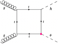
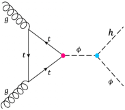
Figure 1: The representative Feynman diagrams for $h\phi$ production in the Higgs alignment limit, where $\phi=H\,{\rm{or}}\,A$ is the additional scalar.

In this work, we extend this strategy to the $h\phi_{l}$ production. The representative Feynman diagrams for the scalar productions are shown in Fig. 1. The left and right diagrams show the top box and triangle-induced contributions, respectively. The magenta vertex in the diagram corresponds to the additional top-Yukawa coupling in Eq. (7), and the cyan one denotes the triple Higgs couplings. The previous experimental data were not enough to probe the new physics scenarios via this production when the additional scalar boson is heavy. However, the expected data at the current and future LHC can shed light on this production as we will show. Note that in the general 2HDM parameter space, for the $h\phi$ production there is another relevant diagram which comes from the $Z$-boson exchange Drell-Yan process. Although it is generated by the EW interaction, thanks to its tree-level nature, its contribution can be potentially much larger than the gluon-fusion process in Fig. 1 according to [91]. Nevertheless, it is important to notice that such EW production is significantly suppressed in the Higgs alignment limit, while the top-loop induced productions are not suppressed.

As a demonstration, we consider a case of $\phi_{l}=A$ and $\phi_{h}=H$. We note that the CP-conserving scalar potential does not allow the $hA$ production through $gg\to h$ or $H\to hA$. Furthermore, the Higgs alignment limit ensures that $gg\to h\to hH$ process vanishes but leaves a non-vanishing triple-Higgs couplings $\lambda_{hAA}$ and $\lambda_{hHH}$; hence $gg\to A\to hA$ and $gg\to H\to hH$ processes are irreducible in the Higgs alignment limit. The representative diagrams are shown in Fig. 1.

In this study, there are four relevant free parameters to the $h\phi_{l}$ production: (1) the produced lighter scalar mass $m_{\phi_{l}}$, (2) the heavier scalar mass $m_{\phi_{h}}$, (3) the triple Higgs coupling $\lambda_{hAA}$ ($\lambda_{hHH}$) for $hA$ ($hH$) production, and (4) the additional top-Yukawa coupling $\rho_{tt}^{\phi}$. In our analysis, we fix $m_{\phi_{l}}$ and $\rho_{tt}^{\phi}$ and vary $m_{\phi_{h}}$ and $\lambda_{3}$ coupling by assuming $m_{H^{\pm}}=m_{\phi_{h}}$ to avoid the experimental bound from the oblique parameter. We numerically calculate the production cross section by MadGraph5_aMC@NLO [107] for a given set of $A$ and $H$ masses and $\lambda_{3}$. For each benchmark parameter point, ten thousand events are generated. It is noted that the matrix elements of one-loop-induced $gg\to hA$ process have been validated against an independent implementation of 2HDM model in OpenLoops2 [109].

In Fig. 2, by fixing $m_{\phi_{l}}=100$ GeV, we show the $h\phi_{l}$ production cross section in the unit of fb and the $\lambda_{h\phi_{l}\phi_{l}}$ in red and blue contours, respectively. The result for $m_{\phi_{l}}=50,\,150,\,200,\,250,\,300\,,400\,$GeV can be found in Appendix A. The vertical and horizontal axes correspond to $\lambda_{3}$ and $m_{\phi_{h}}$. We set $\rho_{tt}^{\phi}=1$ for simplicity since both the amplitudes corresponding to diagrams in Fig. 1 are linearly proportional to $\rho_{tt}^{\phi}$. The cross section is proportional to $|\rho_{tt}^{\phi}|^{2}$, thus it is easy to rescale the cross section.

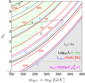
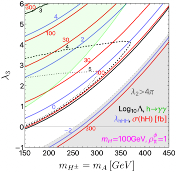
Figure 2: The $h\phi_{l}$ production cross section is shown in red contours on the heavier scalar mass and $\lambda_{3}$ plane. The lighter scalar mass is fixed as $m_{A}=100\,$GeV (left) and $m_{H}=100\,$GeV (right). The figures with other masses are found in Appendix A. Blue contours denote $\lambda_{hAA}$ and $\lambda_{hHH}$ at the additional scalar scale. The light green region and gray regions are excluded by the $h\to\gamma\gamma$ constraint and the vacuum stability condition, respectively. The black contours show the cutoff scale in Log${}_{10}(\Lambda$/GeV).

The relevant constraints on $\rho_{tt}^{\phi}$, which depends on the scalar mass spectrum, are discussed in Sec. 3.2. Combining those constraints and production cross section in Figs. 2, 4 and 5, the realistic production cross section can be obtained. We observed that the SM-like destructive interference among the diagrams in Fig. 1 exists in the $hA$ as well as the $hH$ production modes. Especially for the $hA$ production, the additional $\gamma_{5}$ insertions play a similar role in the Dirac algebra of loop numerators in the box and triangle diagrams, hence the destructive interference is expected. Our numerical analysis explicitly shows the destructive behavior in the parameter regions with $\lambda_{h\phi_{l}\phi_{l}}>0$. It is observed that the production cross section can be $\mathcal{O}(100)$ fb for $m_{\phi_{l}}=100\,$GeV with $\rho_{tt}^{\phi}=1$. For $m_{\phi_{l}}=400\,$GeV the cross section can be $\mathcal{O}(10)$ fb. We see that the cancellation occurs when $\lambda_{h\phi_{l}\phi_{l}}$ is of $\mathcal{O}(1)$.

Given the similarity between $h\phi$ production and the SM $hh$ production at the leading order and the fact that higher-order QCD corrections do not introduce additional $\gamma_{5}$ insertions, we further expect that a SM-like NLO QCD $K$-factor is around 2 for the loop-induced $gg\to h\phi$ cross sections as well. This $K$-factor $\simeq 2$ is partially confirmed in Ref. [93] in the heavy top-mass limit, and it is important to confirm this expectation in the future by exact calculations which are out of the scope of this paper.

Furthermore, the Higgs precision data can constrain the parameter space. While most of the Higgs signal strengths approach the SM Higgs predictions in the Higgs alignment limit, the signal strength for $\gamma\gamma$ does not. It is because the one-loop induced charged scalar contribution modifies $h\to\gamma\gamma$ rate, which has been measured with LHC Run 2 full data [110]. The light green region in Fig. 2 is excluded at the $2\sigma$ level. This constraint is especially relevant for the low-mass $H^{\pm}$ region with large coupling $\lambda_{3}$. On the other hand, one could also consider the $pp\to\phi_{l}\to\gamma\gamma$ search. However, the value of BR$(\phi_{l}\to\gamma\gamma)$ significantly depends on the Yukawa couplings $\rho_{tt}^{\phi}$, $\rho_{\tau\tau}^{\phi}$ and also $\rho_{bb}^{\phi}$. So, we conclude that the constraint from the $pp\to\phi_{l}\to\gamma\gamma$ search is reducible in Fig. 2. Note that when one chooses the appropriate size of Yukawa couplings, the CMS di-photon excess [82] can be explained by $pp\to\phi_{l}\to\gamma\gamma$ [84].

If the trilinear scalar couplings are too large, they eventually blow up at high energies due to the renormalization group evolution. We consider a perturbative unitarity bound [111, 112, 113] where the renormalization group evolution effect is considered based on Refs. [114, 115]. Here, we set $\lambda_{7}=0$ as a reference value. When one takes $\lambda_{7}=\mathcal{O}(1)$ which is an irrelevant parameter to $h\phi_{l}$ production, the unitarity bound becomes more severe. The black solid, dashed and dotted lines in Fig. 2 corresponds to the cutoff scale of $\Lambda=10^{3},10^{4}$ and $10^{5}\,{\rm{GeV}}$, respectively. If one requires the model to be perturbative up to $10$ TeV, then the region outside the black dashed line will be excluded.

Another theoretical constraint on the quartic couplings comes from the vacuum stability of the scalar potential. In this paper, we impose the tree-level bounded-from-below condition for the scalar potential [116, 117],

$$\lambda_{1},\lambda_{2}>0\,,\quad\sqrt{\lambda_{1}\lambda_{2}}+\lambda_{3}>0\,,\quad\sqrt{\lambda_{1}\lambda_{2}}+\lambda_{3}+\lambda_{4}-|\lambda_{5}|>0\,.$$ (8)

In order to produce a large mass difference between $\phi_{l}$ and $\phi_{h}$, $\lambda_{4}$ must be largely negative value at the EW scale. Therefore, to satisfy the last condition in Eq. (8), $\lambda_{2}$ must be largely positive, though it does not change the phenomenology discussed in this paper. The gray region in Fig. 2 is excluded since there $\lambda_{2}$ becomes too large ($\lambda_{2}>4\pi$) to respect the bounded-from-bellow condition [118]. We see that various constraints are very complementary on this plane.

3.2 Constraints on $\rho_{tt}^{\phi}$

In this section, we discuss the relevant flavor and collider constraints on the top-Yukawa couplings. First of all, we summarize the constraints from the direct searches at the LHC. The $tb$ resonance search is relevant for the additional charged scalar $H^{\pm}$, and the $t\overline{t}$ resonance search is relevant for the extra neutral scalars $H$ and $A$ when $\rho_{tt}^{\phi}$ is dominant among the interactions. On the other hand, since a bound from the $\tau\overline{\tau}$ resonance search strongly depends on whether the scalar has other decay modes or not, we consider only the case where $\rho_{tt}^{\phi}$ is dominant compared to other couplings for simplicity.

In Fig. 3, we derive the upper limit on $\rho_{tt}^{\phi}$ as a function of $m_{H^{\pm}}\,(=m_{\phi_{h}})$. The orange region is excluded by the $pp\to tbH^{\pm}\to\bar{t}bt\bar{b}$ process based on the LHC Run 2 full data [119] assuming $\text{BR}(H^{\pm}\to tb)=1$. It is noted that the experimental data is available in the region of $m_{H^{\pm}}\geq 200\,$GeV. In fact, there is also a decay mode where the scalar decays into gauge bosons $H^{\pm}\to W^{\pm}\phi_{l}$, and the $\bar{t}b$ branching fraction is diluted for $m_{H^{\pm}}-m_{\phi_{l}}>m_{W}$. For instance, we obtain $\text{BR}(H^{\pm}\to tb)=0.6$ for $\rho_{tt}^{\phi}=1$ with $m_{H^{\pm}}=350$ GeV and $m_{\phi_{l}}=100$ GeV. Notice that the dilution of the bound significantly depends on $m_{\phi_{l}}$.

Another collider constraint for a light $H^{\pm}$ scenario comes from the exotic top decay which is available in the range of $m_{H^{\pm}}\leq 160\,$GeV. If the couplings other than $\rho_{tt}^{\phi}$ are negligible for $m_{H^{\pm}}\leq m_{t}$, then $H^{\pm}\to cb$ will be the dominant decay mode via $\rho^{d}_{bb}$ or $\rho^{u}_{tc}$ interactions in Eq. (6). Both ATLAS and CMS collaborations have searched for $H^{\pm}\to cb$ channel via a top quark decay [120, 121], and they set the upper limit on the product of $\text{BR}(t\to bH^{\pm})\times\text{BR}(H^{\pm}\to bc)$ as a function of $m_{H^{\pm}}$. Assuming $\text{BR}(H^{\pm}\to cb)=1$, we can set the upper limit on $\rho_{tt}^{\phi}$ which is shown by the blue region in Fig. 3. Similarly, if $H^{\pm}\to\tau\nu$ is the dominant decay mode via scalar-tau Yukawa interaction, we can set the upper limit on $\rho_{tt}^{\phi}$ which is shown by the purple region in Fig. 3 [122]. Furthermore, the similar upper limit can be obtained from $H^{\pm}\to cs$ via $\rho^{u}_{cc}$ and $\rho^{d}_{ss}$ [123]. It is noted that $t\overline{t}$ resonance and four-top searches give a weaker constraint [124], and thus they are omitted.

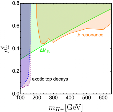
Figure 3: The upper limit on $\rho_{tt}^{\phi}$ as a function of $m_{H^{\pm}}$ at 95$\%$ CL. Orange region is excluded by the $tb$ resonance search. Purple and blue regions surrounded by dotted lines could be disfavored by the $t\to bH^{\pm}\to b\tau\nu$ and $t\to bH^{\pm}\to bbc$ decays, respectively. The light green region is excluded by the $B_{s}$-meson mixing bound.

The large $\rho_{tt}^{\phi}$ also modifies the $B_{(s)}$-meson mixing $\Delta M_{B_{(s)}}$ at one-loop level. We use the analytic formula for the $H^{\pm}$ box contribution ($H^{\pm}$-$W^{\mp}$ and $H^{\pm}$-$H^{\mp}$ boxes) from Refs. [125, 126] and adopt the latest bound [127]. The renormalization group running correction from $\mu=m_{H^{\pm}}$ to $\mu=m_{W}$ is taken into account. Notice that other flavor constraints, for example, the ones from $b\to s\gamma$ and semileptonic decays of kaon, are confirmed to be less stringent [128]. In Fig. 3, the light green region is excluded by the $B_{s}$ mixing constraint. Since the $B_{s}$ mixing constraint does not depend on $m_{\phi_{l}}$ and the decay modes, the bound is the most conservative in Fig. 3. It is observed that the mass gap exists for the LHC bounds around $m_{H^{\pm}}\sim m_{t}$ due to the experimental difficulty. However, the $B_{s}$ mixing constraint is complementary and thus fills the gap.

It is observed that for example, $\rho_{tt}^{\phi}\simeq 0.4$ is allowed for the $m_{H^{\pm}}\gtrsim 200$ GeV scenario. Combining these constraints with Figs. 2, 4 and 5, one can read the maximal production cross section of the $h\phi_{l}$ channels as we will show an example in the next section.

It is worth mentioning that in addition to the $\rho^{\phi}_{tt}$ bound, a severe constraint on $\lambda_{h\phi_{l}\phi_{l}}$ appears for $m_{\phi_{l}}\leq m_{h}/2$ in Fig. 4. In this parameter region, the $h\to\phi_{l}\phi_{l}$ decay is kinematically open and modifies the Higgs total width. The partial decay width is given as

$$\Gamma(h\to\phi_{l}\phi_{l})=\frac{\lambda_{h\phi_{l}\phi_{l}}^{2}v^{2}}{32\pi m_{h}}\sqrt{1-\frac{4m_{\phi_{l}}^{2}}{m_{h}^{2}}}\,.$$ (9)

The current bound [129, 130] corresponds to $\lambda_{h\phi_{l}\phi_{l}}\leq{\mathcal{O}}(10^{-2})$ for $m_{\phi_{l}}\leq m_{h}/2$.

3.3 Comment on solutions of di-tau excess and muon $g-2$

In this subsection, we briefly discuss the phenomenological impacts on the di-tau excess and the muon $g-2$ anomaly explanations in the 2HDMs.

Since the 100 GeV $\tau\bar{\tau}$ excess requires an additional light scalar decaying into di-tau final states, we introduce the following interaction,

$$-\mathcal{L}_{\rm Yukawa}^{\tau}=\frac{\rho_{\tau\tau}^{\phi}}{\sqrt{2}}\,\bar{\tau}H\tau+i\frac{\rho_{\tau\tau}^{\phi}}{\sqrt{2}}\,\bar{\tau}A\gamma_{5}\tau\,.$$ (10)

It is shown in Ref. [84] that the a simultaneous explanation of the di-tau [81] and di-photon excesses [82] favors $m_{\phi_{l}}=m_{A}\simeq 95\text{--}100$ GeV with $\rho_{tt}^{\phi}\simeq 0.4$ and $\rho_{\tau\tau}^{\phi}\simeq 3\times 10^{-3}$, which corresponds to $\text{BR}(A\to\tau\overline{\tau})\simeq 0.3$. As seen from Fig. 3 that $m_{H^{\pm}}\leq$ 200 GeV with $\rho_{tt}^{\phi}\simeq 0.4$ can not satisfy the $\Delta M_{B_{s}}$ bound. Furthermore, we found that $m_{H}\leq 2m_{t}$ is excluded by the di-tau search [131]. For $m_{H}\geq 2m_{t}$, $\text{BR}(H\to\tau\overline{\tau})$ is significantly diluted and the bound becomes weak, thus the explanation is possible.

On the other hand, the current $95\%$ CL upper limits on the signal strengths of the di-Higgs production in $b\overline{b}\tau\overline{\tau}$ decay mode is given as $\mu(hh\to b\overline{b}\tau\overline{\tau})\leq 3.3$ [132]. The NNLO SM prediction is given as $\sigma_{\rm ggF}^{hh}=31.05^{+6\%}_{-23\%}\pm 3\%$ fb with $m_{h}=125\,$GeV [23, 133]. It is noted that the experimental upper limit is a consequence of the combination of gluon fusion (ggF) and vector boson fusion (VBF). Although the VBF cross section is small, $\sigma_{\rm VBF}^{hh}=1.73^{+0.03\%}_{-0.04\%}\pm 2.1\%$ fb at NNLO [133], the unique VBF event topology provides a useful handle to identify signal events and sensitivity. While it is nontrivial to separate the impacts of ggF and VBF determination, the ggF mainly determines the upper limit [132]. With the SM predictions $\text{BR}(h\to b\overline{b})=58.1\%$ and $\text{BR}(h\to\tau\overline{\tau})=6.3\%$, we can estimate a rough sensitivity of $hA$ production at the LHC by only considering the ggF mode, and the current LHC data reaches $7.5\,\rm{fb}$ for the di-Higgs production with $b\overline{b}\tau\overline{\tau}$ final state.

From Fig. 2, we can see that $\sigma(pp\to hA)$ is as large as $200$ fb for $\rho_{tt}^{\phi}=1$ when the cutoff scale $\Lambda>10$ TeV is imposed. For $\rho_{tt}^{\phi}=0.4$, the production cross section is calculated as $\sigma(pp\to hA)=200\times 0.4^{2}\simeq 30$ fb. Therefore the explanation of $\tau\overline{\tau}$ excess with $m_{A}\sim 100$GeV, $\rho_{tt}^{\phi}=0.4$, $\rho_{\tau\tau}^{\phi}=3\times 10^{-3}$ predicts $\sigma(pp\to hA)\times\text{BR}(h\to b\overline{b})\times\text{BR}(A\to\tau\overline{\tau})\simeq 5.6$ fb, which is larger than the SM di-Higgs prediction ($2.3$ fb). If the $K$-factor is about 2 for $\sigma(pp\to hA)$, then the model prediction exceeds the current exclusion for the $hh$ channel. As shown in Ref. [84], unlike the CP-even interpretation, it is challenging to test the CP-odd solution for the $\tau\bar{\tau}$ excess in $t\bar{t}+\tau\bar{\tau}$ final state, whereas the $hA$ production (decaying into $b\overline{b}\tau\overline{\tau}$) allows us probe this solution. In this context, more dedicated sensitivity studies are necessary from both experimental and theoretical sides. It is noted that the single $H$ production process can be relevant for the model parameter space. The CMS collaboration probed $pp\to H\to AZ\to\tau\bar{\tau}+l\bar{l}$ process with the Run 1 data and the $\mathcal{O}(10)$ fb upper limit on $\sigma(pp\to H\to AZ\to\tau\bar{\tau}+l\bar{l})$ has been set. We calculated the signal cross section based on the SusHi [136, 137] and confirmed that the parameter which explains $\tau\tau$ and di-photon excesses simultaneously predicts the smaller signal cross section by roughly a factor of $1/2$. The LHC Run 2 full result would give conclusive evidence.

It is known that a light pseudo scalar is necessary for an explanation of the muon $g-2$ anomaly in the type-X and flavor-aligned (FA-) 2HDMs [80], where the dominant contribution comes from the two-loop Barr-Zee diagram with tau loop. In the type-X 2HDM, the top-Yukawa coupling with the heavy scalar is $\mathcal{O}(0.01)$ for the excess favored region. Therefore, the di-Higgs production cross-section is too small to be observed. We also found that even in the FA-2HDM, the top-Yukawa coupling can not be large due to the constraint from $B_{s}\to\mu\bar{\mu}$ measurement that is enhanced with a light scalar exchange diagram [138]. Furthermore, it would not be easy to reconstruct the additional light scalar in $\tau\bar{\tau}$ final state at the LHC due to several neutrinos. Therefore, we conclude that the di-Higgs production for the solution of the muon $g-2$ anomaly is less relevant.

4 Conclusion

The Higgs field plays a very important role in giving masses to the SM particles. However, there are still open questions, for example, the origins of the negative mass term and also the hierarchy of the fermions. There would be new physics to solve the questions. On the other hand, it is known that the extended Higgs models can be the key to explaining the origins of the neutrino masses, EW baryogenesis, dark matter, and EW vacuum stability. Therefore it is often believed that the study of the Higgs sector is the way to access physics beyond the SM. The 2HDM is one of the simplest extensions of the SM that frequently appears in new physics scenarios. It is known that this model can explain the excesses in the $\tau\bar{\tau}$ and $\gamma\gamma$ resonances data reported by the CMS collaboration as well as the muon $g-2$ anomaly. Those discrepancies require a light neutral scalar which will be within the reach of the LHC. This kind of light scalar is also well motivated by a successful strong first-order EW phase transition and the baryon asymmetry of the Universe.

In order to chase a realistic and still-allowed 2HDM that can resolve the aforementioned puzzles, in this paper, we investigated the $h\phi$ production where $\phi$ is the additional neutral scalar ($\phi=H,\,A$). This process will be interesting in the HL-LHC era. We calculated the cross section of $h\phi$ production from the loop-induced gluon fusion channel at the leading order. We took into account the theoretical bounds from the perturbative unitarity and vacuum stability conditions, and the experimental bounds from the Higgs and flavor precision measurements as well as the direct search at the LHC. It is found that $h\phi$ production cross section could be as large as $\mathcal{O}(30)$ fb if the additional scalar mass is around 100 GeV. One should note that $\phi\phi$ production (would decay into $4\tau$, which is harder to probe than 2$b$2$\tau$ from $h\phi_{l}$ production) can also be a relevant search channel. Although the top-loop box contribution is suppressed by an additional factor of $\rho^{\phi}_{tt}$, $gg\to h\to\phi\phi$ and $gg\to\phi\to\phi\phi$ contributions are not, and the latter depends on the value of $\lambda_{7}$ and also the resonance enhancement is possible.

Furthermore, motivated by the low mass $\tau\bar{\tau}$ and $\gamma\gamma$ resonant excesses reported by the CMS collaboration, we investigated the impact of the $h\phi$ production. It was found that the combined explanation of the excesses predicts $\sigma(pp\to hA\to b\bar{b}\tau\bar{\tau})\simeq 6\,$fb at the QCD leading order. Very interestingly, this leading-order cross section is already larger than the SM Higgs-pair production decaying into $b\overline{b}\tau\overline{\tau}$ by a factor of more than two. Therefore, this mode provides a unique window to probe the possible explanation of the excesses. Lastly, it is clear that more dedicated precise calculations and experimental simulations to evaluate the realistic sensitivity are further needed.

Appendix A Additional figures

In this Appendix, we present figures that are not shown in the main text. Figure 4 shows the production cross sections for $m_{\phi_{l}}=50$ GeV (upper), 150 GeV (middle) and 200 GeV (bottom). Figure 5 shows the results for $m_{\phi_{l}}=250$ GeV (upper), 300 GeV (middle) and 400 GeV (bottom). The color code is the same as Fig. 2 and for the description of the contours see the caption of Fig. 2 and the main text. For $m_{\phi_{l}}=50\,$GeV, the Higgs width bound gives a stringent constraint on $\lambda_{h\phi_{l}\phi_{l}}$ since $h\to\phi_{l}\phi_{l}$ is kinematically open. Therefore, the allowed region from the Higgs width bound must be almost degenerated to the line of $\lambda_{h\phi_{l}\phi_{l}}=0$. It is noted that the constraint from $h\to\gamma\gamma$ does not appear on the plane with $m_{\phi_{l}}=400\,$GeV. As mentioned in Sec. 3.1, these cross-section data are available in [108].

​​​​​​     

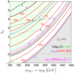
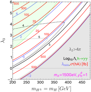
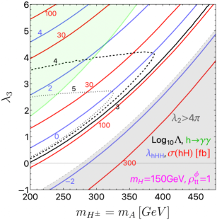
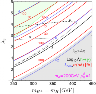
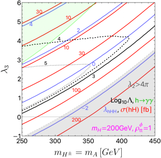
Figure 4: The $h\phi_{l}$ production cross section is shown on the heavier scalar mass vs. $\lambda_{3}$ plane. The left and right figures are for $hA$ and $hH$ productions, respectively. The lighter scalar mass is fixed to be 50 GeV (upper), 150 GeV (middle), 200 GeV (bottom). See, the caption of Fig. 2 for the description of the constraints and other explanations.

​​​​​   

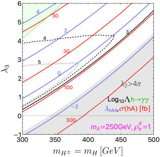
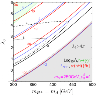
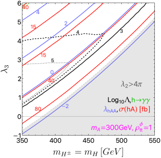
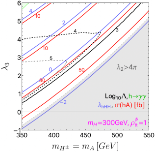
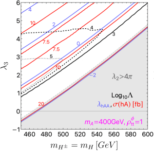
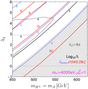
Figure 5: The $h\phi_{l}$ production cross section is shown on the heavier scalar mass vs. $\lambda_{3}$ plane. The left and right figures are for $hA$ and $hH$ productions, respectively. The lighter scalar mass is fixed to be 250 GeV (upper), 300 GeV (middle), 400 GeV (bottom). See, the caption of Fig. 2 for the description of the constraints and other explanations.

Appendix B Parameter relations in the 2HDMs

For the sake of completeness, in this Appendix, we summarize the parameter relations between the general basis and the Higgs basis in the 2HDMs (see, e.g., Refs. [139, 125, 140]).

The most general Higgs potential for the general 2HDM is given by

$$V=~{} m_{11}^{2}\Phi_{1}^{\dagger}\Phi_{1}+m_{22}^{2}\Phi_{2}^{\dagger}\Phi_{2}-\left(m_{12}^{2}\Phi_{1}^{\dagger}\Phi_{2}+\text{h.c.}\right)$$

$$+\frac{1}{2}\lambda_{1}^{G}\left(\Phi_{1}^{\dagger}\Phi_{1}\right)^{2}+\frac{1}{2}\lambda_{2}^{G}\left(\Phi_{2}^{\dagger}\Phi_{2}\right)^{2}+\lambda_{3}^{G}\left(\Phi_{1}^{\dagger}\Phi_{1}\right)\left(\Phi_{2}^{\dagger}\Phi_{2}\right)+\lambda_{4}^{G}\left(\Phi_{1}^{\dagger}\Phi_{2}\right)\left(\Phi_{2}^{\dagger}\Phi_{1}\right)$$

$$+\left\{\frac{1}{2}\lambda_{5}^{G}\left(\Phi_{1}^{\dagger}\Phi_{2}\right)^{2}+\left[\lambda_{6}^{G}\left(\Phi_{1}^{\dagger}\Phi_{1}\right)+\lambda_{7}^{G}\left(\Phi_{2}^{\dagger}\Phi_{2}\right)\right]\left(\Phi_{1}^{\dagger}\Phi_{2}\right)+\text{h.c.}\right\}\,,$$ (11)

with

$$\Phi_{i} =\begin{pmatrix}\omega_{i}^{+}\\ \frac{1}{\sqrt{2}}\left(v_{i}+h_{i}+iz_{i}\right)\end{pmatrix}\,,\quad(i=1,\,2)\,,$$ (12)

where $v_{i}/\sqrt{2}$ is the VEV of $\Phi_{i}^{0}$, satisfying $v=\sqrt{v_{1}^{2}+v_{2}^{2}}=(\sqrt{2}G_{F})^{-1/2}\simeq 246\,\text{GeV}$ and $\tan\beta={v_{2}}/{v_{1}}$. Both $v_{i}$ can be taken to be real and positive values without losing generality. On the other hand, $m_{12}^{2}$ and $\lambda_{5,6,7}^{G}$ are complex values in general. When one imposes the softly-broken $\mathbbm{Z}_{2}$ symmetry ($\Phi_{1}\to\Phi_{1},~{}\Phi_{2}\to-\Phi_{2}$) to prohibit the flavor-changing neutral currents, $\lambda^{G}_{6,7}$ must be set to zero for any renormalization scale.

In the following, we assume the CP conservation for simplicity, and then $m_{12}^{2}$ and $\lambda_{5,6,7}^{G}$ are real. The stationary conditions for the general 2HDM potential are

$$\begin{aligned} m_{11}^{2}-s^{2}_{\beta}M^{2}+\frac{v^{2}}{2}\left(c_{\beta}^{2}\lambda_{1}^{G}+s_{\beta}^{2}\lambda^{G}_{345}+3s_{\beta}c_{\beta}\lambda_{6}^{G}+s^{2}_{\beta}\tan\beta\lambda_{7}^{G}\right)&=0\,,\\ m_{22}^{2}-c^{2}_{\beta}M^{2}+\frac{v^{2}}{2}\left(s_{\beta}^{2}\lambda_{2}^{G}+c_{\beta}^{2}\lambda^{G}_{345}+c_{\beta}^{2}\cot\beta\lambda^{G}_{6}+3s_{\beta}c_{\beta}\lambda^{G}_{7}\right)&=0\,,\end{aligned}$$ (13)

with

$$M^{2}=\frac{m_{12}^{2}}{s_{\beta}c_{\beta}}\,,\quad\lambda^{G}_{345}=\lambda^{G}_{3}+\lambda^{G}_{4}+\lambda^{G}_{5}\,,$$ (14)

where $s_{\beta}=\sin\beta$ and $c_{\beta}=\cos\beta$.

The Higgs basis in Eq. (2) is obtained by

$$\left(\begin{array}[]{l}H_{1}\\ H_{2}\end{array}\right)=\left(\begin{array}[]{cc}c_{\beta}&s_{\beta}\\ -s_{\beta}&c_{\beta}\end{array}\right)\left(\begin{array}[]{l}\Phi_{1}\\ \Phi_{2}\end{array}\right)\,.$$ (21)

By matching the scalar potential in Eq. (11) to the one in the Higgs basis (1), we obtain the following parameter relations:

$$M_{11}^{2} =c^{2}_{\beta}m_{11}^{2}+s^{2}_{\beta}m_{22}^{2}-s_{2\beta}m_{12}^{2}\,,$$ (22)

$$M_{22}^{2} =s^{2}_{\beta}m_{11}^{2}+c^{2}_{\beta}m_{22}^{2}+s_{2\beta}m_{12}^{2}\,,$$ (23)

$$M_{12}^{2} =\frac{1}{2}s_{2\beta}\left(m_{11}^{2}-m^{2}_{22}\right)+c_{2\beta}m_{12}^{2}\,,$$ (24)

$$\lambda_{1} =c^{4}_{\beta}\lambda_{1}^{G}+s^{4}_{\beta}\lambda_{2}^{G}+\frac{1}{2}s^{2}_{2\beta}\lambda^{G}_{345}+2s_{2\beta}\left(c_{\beta}^{2}\lambda_{6}^{G}+s_{\beta}^{2}\lambda_{7}^{G}\right)\,,$$ (25)

$$\lambda_{2} =s^{4}_{\beta}\lambda_{1}^{G}+c^{4}_{\beta}\lambda_{2}^{G}+\frac{1}{2}s^{2}_{2\beta}\lambda_{345}^{G}-2s_{2\beta}\left(s_{\beta}^{2}\lambda_{6}^{G}+c_{\beta}^{2}\lambda_{7}^{G}\right)\,,$$ (26)

$$\lambda_{3} =\frac{1}{4}s^{2}_{2\beta}\left(\lambda_{1}^{G}+\lambda_{2}^{G}-2\lambda_{345}^{G}\right)+\lambda_{3}^{G}-\frac{1}{2}s_{4\beta}\left(\lambda_{6}^{G}-\lambda_{7}^{G}\right)\,,$$ (27)

$$\lambda_{4} =\frac{1}{4}s^{2}_{2\beta}\left(\lambda_{1}^{G}+\lambda_{2}^{G}-2\lambda_{345}^{G}\right)+\lambda_{4}^{G}-\frac{1}{2}s_{4\beta}\left(\lambda_{6}^{G}-\lambda_{7}^{G}\right)\,,$$ (28)

$$\lambda_{5} =\frac{1}{4}s^{2}_{2\beta}\left(\lambda_{1}^{G}+\lambda_{2}^{G}-2\lambda_{345}^{G}\right)+\lambda_{5}^{G}-\frac{1}{2}s_{4\beta}\left(\lambda_{6}^{G}-\lambda_{7}^{G}\right)\,,$$ (29)

$$\lambda_{6} =-\frac{1}{2}s_{2\beta}\left(c^{2}_{\beta}\lambda^{G}_{1}-s^{2}_{\beta}\lambda^{G}_{2}-c_{2\beta}\lambda^{G}_{345}\right)+c_{\beta}^{2}\left(1-4s_{\beta}^{2}\right)\lambda_{6}^{G}+s_{\beta}^{2}\left(-1+4c_{\beta}^{2}\right)\lambda_{7}^{G}\,,$$ (30)

$$\lambda_{7} =-\frac{1}{2}s_{2\beta}\left(s^{2}_{\beta}\lambda_{1}^{G}-c^{2}_{\beta}\lambda_{2}^{G}+c_{2\beta}\lambda_{345}^{G}\right)+s_{\beta}^{2}\left(-1+4c_{\beta}^{2}\right)\lambda_{6}^{G}+c_{\beta}^{2}\left(1-4s_{\beta}^{2}\right)\lambda_{7}^{G}\,.$$ (31)

Using the stationary equations (13), $M_{11}^{2}$ and $M_{12}^{2}$ can be represented as

$$M_{11}^{2} =-\frac{v^{2}}{2}\left(c_{\beta}^{4}\lambda_{1}^{G}+s_{\beta}^{4}\lambda_{2}^{G}+\frac{1}{2}s_{2\beta}^{2}\lambda_{345}^{G}+4c_{\beta}^{3}s_{\beta}\lambda_{6}^{G}+4s_{\beta}^{3}c_{\beta}\lambda_{7}^{G}\right)$$

$$=-\frac{1}{2}\lambda_{1}v^{2}\,,$$ (32)

$$M_{12}^{2} =\frac{v^{2}}{2}\left[-\frac{1}{2}s_{2\beta}\left(c_{\beta}^{2}\lambda_{1}^{G}-s_{\beta}^{2}\lambda_{2}^{G}-c_{2\beta}\lambda_{345}^{G}\right)+c_{\beta}^{2}\left(1-4s_{\beta}^{2}\right)\lambda_{6}^{G}+s_{\beta}^{2}\left(-1+4c_{\beta}^{2}\right)\lambda_{7}^{G}\right]$$

$$=\frac{1}{2}\lambda_{6}v^{2}\,.$$ (33)

When one imposes the approximate Higgs alignment condition ($\lambda_{6}\simeq 0$) in order to avoid the experimental bounds from measurements of the Higgs signal strengths, the scalar potential is given as

$$\begin{aligned} V\simeq&-\frac{1}{2}\lambda_{1}v^{2}H_{1}^{\dagger}H_{1}+M_{22}^{2}H_{2}^{\dagger}H_{2}\\ &+\frac{\lambda_{1}}{2}(H_{1}^{\dagger}H_{1})^{2}+\frac{\lambda_{2}}{2}(H_{2}^{\dagger}H_{2})^{2}+\lambda_{3}(H_{1}^{\dagger}H_{1})(H_{2}^{\dagger}H_{2})+\lambda_{4}(H_{1}^{\dagger}H_{2})(H_{2}^{\dagger}H_{1})\\ &+\left[\frac{\lambda_{5}}{2}(H_{1}^{\dagger}H_{2})^{2}+\lambda_{7}(H_{2}^{\dagger}H_{2})(H_{1}^{\dagger}H_{2})+{\rm h.c.}\right]\,.\end{aligned}$$ (34)

The scalar boson masses are determined as

$$\begin{aligned} m_{h}^{2}&\simeq\lambda_{1}v^{2}\,,\quad&m_{H}^{2}&\simeq M_{22}^{2}+\frac{1}{2}\lambda_{345}v^{2}\,,\\ m_{A}^{2}&=M_{22}^{2}+\frac{1}{2}\left(\lambda_{3}+\lambda_{4}-\lambda_{5}\right)v^{2}\,,\quad&m_{H^{\pm}}^{2}&=M_{22}^{2}+\frac{1}{2}\lambda_{3}v^{2}\,.\end{aligned}$$ (35)

Given four scalar boson masses, the remaining degrees of freedom in this model are three (e.g., $\lambda_{2,3,7}$), and the value of $\lambda_{7}$ is irrelevant to our study except for an indirect effect on the perturbative unitarity bound. As we discussed below Eq. (8), $\lambda_{2}$ gives only a relevant effect on the vacuum stability condition. As a consequence, the production cross-section of $gg\to h\phi_{l}$ can be determined only by $\lambda_{3}$ and the scalar masses.

When one imposes the (softly-broken) $\mathbbm{Z}_{2}$ symmetry, $\lambda_{6,7}^{G}$ are forbidden. This condition provides the following parameter relations in the Higgs basis:

$$\lambda_{6}^{G} =\frac{1}{2}s_{2\beta}\left(c_{\beta}^{2}\lambda_{1}-s_{\beta}^{2}\lambda_{2}-c_{2\beta}\lambda_{345}\right)+c_{\beta}c_{3\beta}\lambda_{6}+s_{\beta}s_{3\beta}\lambda_{7}=0\,,$$ (36)

$$\lambda_{7}^{G} =\frac{1}{2}s_{2\beta}\left(s_{\beta}^{2}\lambda_{1}-c_{\beta}^{2}\lambda_{2}+c_{2\beta}\lambda_{345}\right)+s_{\beta}s_{3\beta}\lambda_{6}+c_{\beta}c_{3\beta}\lambda_{7}=0\,,$$ (37)

which further restrict the parameters. Note that in this paper we do not impose these conditions.

References

- [1] S. L. Glashow, “Partial Symmetries of Weak Interactions,” Nucl. Phys. 22 (1961) 579–588.
- [2] J. Goldstone, A. Salam, and S. Weinberg, “Broken Symmetries,” Phys. Rev. 127 (1962) 965–970.
- [3] P. W. Higgs, “Broken Symmetries and the Masses of Gauge Bosons,” Phys. Rev. Lett. 13 (1964) 508–509.
- [4] F. Englert and R. Brout, “Broken Symmetry and the Mass of Gauge Vector Mesons,” Phys. Rev. Lett. 13 (1964) 321–323.
- [5] G. S. Guralnik, C. R. Hagen, and T. W. B. Kibble, “Global Conservation Laws and Massless Particles,” Phys. Rev. Lett. 13 (1964) 585–587.
- [6] LHC Higgs Cross Section Working Group Collaboration, “Handbook of LHC Higgs Cross Sections: 4. Deciphering the Nature of the Higgs Sector.” arXiv:1610.07922.
- [7] M. Cepeda et al., “Report from Working Group 2: Higgs Physics at the HL-LHC and HE-LHC,” CERN Yellow Rep. Monogr. 7 (2019) 221–584 [arXiv:1902.00134].
- [8] S. Dawson, S. Dittmaier, and M. Spira, “Neutral Higgs boson pair production at hadron colliders: QCD corrections,” Phys. Rev. D 58 (1998) 115012 [hep-ph/9805244].
- [9] J. Grigo, J. Hoff, K. Melnikov, and M. Steinhauser, “On the Higgs boson pair production at the LHC,” Nucl. Phys. B 875 (2013) 1–17 [arXiv:1305.7340].
- [10] S. Borowka, et al., “Higgs Boson Pair Production in Gluon Fusion at Next-to-Leading Order with Full Top-Quark Mass Dependence,” Phys. Rev. Lett. 117 (2016) 012001 [arXiv:1604.06447]. [Erratum: Phys.Rev.Lett. 117, 079901 (2016)].
- [11] S. Borowka, et al., “Full top quark mass dependence in Higgs boson pair production at NLO,” JHEP 10 (2016) 107 [arXiv:1608.04798].
- [12] R. Gröber, A. Maier, and T. Rauh, “Reconstruction of top-quark mass effects in Higgs pair production and other gluon-fusion processes,” JHEP 03 (2018) 020 [arXiv:1709.07799].
- [13] J. Baglio, et al., “Gluon fusion into Higgs pairs at NLO QCD and the top mass scheme,” Eur. Phys. J. C 79 (2019) 459 [arXiv:1811.05692].
- [14] J. Davies, G. Mishima, M. Steinhauser, and D. Wellmann, “Double Higgs boson production at NLO in the high-energy limit: complete analytic results,” JHEP 01 (2019) 176 [arXiv:1811.05489].
- [15] R. Bonciani, G. Degrassi, P. P. Giardino, and R. Gröber, “Analytical Method for Next-to-Leading-Order QCD Corrections to Double-Higgs Production,” Phys. Rev. Lett. 121 (2018) 162003 [arXiv:1806.11564].
- [16] X. Xu and L. L. Yang, “Towards a new approximation for pair-production and associated-production of the Higgs boson,” JHEP 01 (2019) 211 [arXiv:1810.12002].
- [17] J. Davies, et al., “Double Higgs boson production at NLO: combining the exact numerical result and high-energy expansion,” JHEP 11 (2019) 024 [arXiv:1907.06408].
- [18] L. Bellafronte, G. Degrassi, P. P. Giardino, R. Gröber, and M. Vitti, “Gluon fusion production at NLO: merging the transverse momentum and the high-energy expansions,” JHEP 07 (2022) 069 [arXiv:2202.12157].
- [19] D. de Florian and J. Mazzitelli, “Higgs Boson Pair Production at Next-to-Next-to-Leading Order in QCD,” Phys. Rev. Lett. 111 (2013) 201801 [arXiv:1309.6594].
- [20] D. de Florian and J. Mazzitelli, “Two-loop virtual corrections to Higgs pair production,” Phys. Lett. B 724 (2013) 306–309 [arXiv:1305.5206].
- [21] J. Grigo, J. Hoff, and M. Steinhauser, “Higgs boson pair production: top quark mass effects at NLO and NNLO,” Nucl. Phys. B 900 (2015) 412–430 [arXiv:1508.00909].
- [22] M. Spira, “Effective Multi-Higgs Couplings to Gluons,” JHEP 10 (2016) 026 [arXiv:1607.05548].
- [23] M. Grazzini, et al., “Higgs boson pair production at NNLO with top quark mass effects,” JHEP 05 (2018) 059 [arXiv:1803.02463].
- [24] M. Gerlach, F. Herren, and M. Steinhauser, “Wilson coefficients for Higgs boson production and decoupling relations to ,” JHEP 11 (2018) 141 [arXiv:1809.06787].
- [25] P. Banerjee, S. Borowka, P. K. Dhani, T. Gehrmann, and V. Ravindran, “Two-loop massless QCD corrections to the four-point amplitude,” JHEP 11 (2018) 130 [arXiv:1809.05388].
- [26] L.-B. Chen, H. T. Li, H.-S. Shao, and J. Wang, “The gluon-fusion production of Higgs boson pair: N3LO QCD corrections and top-quark mass effects,” JHEP 03 (2020) 072 [arXiv:1912.13001].
- [27] J. Davies, F. Herren, G. Mishima, and M. Steinhauser, “Real-virtual corrections to Higgs boson pair production at NNLO: three closed top quark loops,” JHEP 05 (2019) 157 [arXiv:1904.11998].
- [28] J. Davies, F. Herren, G. Mishima, and M. Steinhauser, “Real corrections to Higgs boson pair production at NNLO in the large top quark mass limit,” JHEP 01 (2022) 049 [arXiv:2110.03697].
- [29] A. H. Ajjath and H.-S. Shao, “N3LO+N3LL QCD improved Higgs pair cross sections,” JHEP 02 (2023) 067 [arXiv:2209.03914].
- [30] S. Borowka, et al., “Probing the scalar potential via double Higgs boson production at hadron colliders,” JHEP 04 (2019) 016 [arXiv:1811.12366].
- [31] J. Davies, G. Mishima, K. Schönwald, M. Steinhauser, and H. Zhang, “Higgs boson contribution to the leading two-loop Yukawa corrections to gg → HH,” JHEP 08 (2022) 259 [arXiv:2207.02587].
- [32] M. Mühlleitner, J. Schlenk, and M. Spira, “Top-Yukawa-induced corrections to Higgs pair production,” JHEP 10 (2022) 185 [arXiv:2207.02524].
- [33] ATLAS Collaboration, “The ATLAS Experiment at the CERN Large Hadron Collider,” JINST 3 (2008) S08003.
- [34] CMS Collaboration, “The CMS Experiment at the CERN LHC,” JINST 3 (2008) S08004.
- [35] CMS Collaboration, “Performance of reconstruction and identification of leptons decaying to hadrons and in pp collisions at 13 TeV,” JINST 13 (2018) P10005 [arXiv:1809.02816].
- [36] ATLAS Collaboration, “ATLAS b-jet identification performance and efficiency measurement with events in pp collisions at TeV,” Eur. Phys. J. C 79 (2019) 970 [arXiv:1907.05120].
- [37] CMS Collaboration, “Search for Higgs boson pair production in events with two bottom quarks and two tau leptons in proton–proton collisions at =13TeV,” Phys. Lett. B 778 (2018) 101–127 [arXiv:1707.02909].
- [38] CMS Collaboration, “Search for resonant and nonresonant Higgs boson pair production in the final state in proton-proton collisions at TeV,” JHEP 01 (2018) 054 [arXiv:1708.04188].
- [39] ATLAS Collaboration, “Search for pair production of Higgs bosons in the final state using proton-proton collisions at TeV with the ATLAS detector,” JHEP 01 (2019) 030 [arXiv:1804.06174].
- [40] ATLAS Collaboration, “Search for Higgs boson pair production in the final state with 13 TeV collision data collected by the ATLAS experiment,” JHEP 11 (2018) 040 [arXiv:1807.04873].
- [41] ATLAS Collaboration, “Search for resonant and non-resonant Higgs boson pair production in the decay channel in collisions at TeV with the ATLAS detector,” Phys. Rev. Lett. 121 (2018) 191801 [arXiv:1808.00336]. [Erratum: Phys.Rev.Lett. 122, 089901 (2019)].
- [42] CMS Collaboration, “Search for nonresonant Higgs boson pair production in the final state at 13 TeV,” JHEP 04 (2019) 112 [arXiv:1810.11854].
- [43] ATLAS Collaboration, “Search for Higgs boson pair production in the decay mode at TeV with the ATLAS detector,” JHEP 04 (2019) 092 [arXiv:1811.04671].
- [44] ATLAS Collaboration, “Search for non-resonant Higgs boson pair production in the final state with the ATLAS detector in collisions at TeV,” Phys. Lett. B 801 (2020) 135145 [arXiv:1908.06765].
- [45] CMS Collaboration, “Search for nonresonant Higgs boson pair production in final states with two bottom quarks and two photons in proton-proton collisions at = 13 TeV,” JHEP 03 (2021) 257 [arXiv:2011.12373].
- [46] ATLAS Collaboration, “Search for Higgs boson pair production in the two bottom quarks plus two photons final state in collisions at TeV with the ATLAS detector,” Phys. Rev. D 106 (2022) 052001 [arXiv:2112.11876].
- [47] CMS Collaboration, “Search for Higgs Boson Pair Production in the Four b Quark Final State in Proton-Proton Collisions at TeV,” Phys. Rev. Lett. 129 (2022) 081802 [arXiv:2202.09617].
- [48] ATLAS Collaboration, “Search for resonant and non-resonant Higgs boson pair production in the decay channel using 13 TeV collision data from the ATLAS detector.” arXiv:2209.10910.
- [49] ATLAS Collaboration, “Measurement prospects of Higgs boson pair production in the final state with the ATLAS experiment at the HL-LHC.”. http://cds.cern.ch/record/2799146.
- [50] S. P. Martin, “A Supersymmetry primer,” Adv. Ser. Direct. High Energy Phys. 18 (1998) 1–98 [hep-ph/9709356].
- [51] G. Degrassi, S. Heinemeyer, W. Hollik, P. Slavich, and G. Weiglein, “Towards high precision predictions for the MSSM Higgs sector,” Eur. Phys. J. C 28 (2003) 133–143 [hep-ph/0212020].
- [52] R. N. Mohapatra and J. C. Pati, “A Natural Left-Right Symmetry,” Phys. Rev. D 11 (1975) 2558.
- [53] ATLAS Collaboration, “Observation of a new particle in the search for the Standard Model Higgs boson with the ATLAS detector at the LHC,” Phys. Lett. B 716 (2012) 1–29 [arXiv:1207.7214].
- [54] CMS Collaboration, “Observation of a New Boson at a Mass of 125 GeV with the CMS Experiment at the LHC,” Phys. Lett. B 716 (2012) 30–61 [arXiv:1207.7235].
- [55] ATLAS, CMS Collaboration, “Measurements of the Higgs boson production and decay rates and constraints on its couplings from a combined ATLAS and CMS analysis of the LHC pp collision data at and 8 TeV,” JHEP 08 (2016) 045 [arXiv:1606.02266].
- [56] ATLAS Collaboration, “A detailed map of Higgs boson interactions by the ATLAS experiment ten years after the discovery,” Nature 607 (2022) 52–59 [arXiv:2207.00092].
- [57] J. M. Cline, “Baryogenesis,” in Les Houches Summer School - Session 86: Particle Physics and Cosmology: The Fabric of Spacetime. 2006. hep-ph/0609145.
- [58] J. M. Cline, K. Kainulainen, and A. P. Vischer, “Dynamics of two Higgs doublet CP violation and baryogenesis at the electroweak phase transition,” Phys. Rev. D 54 (1996) 2451–2472 [hep-ph/9506284].
- [59] N. Turok and J. Zadrozny, “Electroweak baryogenesis in the two doublet model,” Nucl. Phys. B 358 (1991) 471–493.
- [60] N. Turok and J. Zadrozny, “Phase transitions in the two doublet model,” Nucl. Phys. B 369 (1992) 729–742.
- [61] S. Kanemura and M. Tanaka, “Strongly first-order electroweak phase transition by relatively heavy additional Higgs bosons,” Phys. Rev. D 106 (2022) 035012 [arXiv:2201.04791].
- [62] K. Fuyuto, W.-S. Hou, and E. Senaha, “Electroweak baryogenesis driven by extra top Yukawa couplings,” Phys. Lett. B 776 (2018) 402–406 [arXiv:1705.05034].
- [63] E. Ma, “Verifiable radiative seesaw mechanism of neutrino mass and dark matter,” Phys. Rev. D 73 (2006) 077301 [hep-ph/0601225].
- [64] M. Aoki, S. Kanemura, and O. Seto, “Neutrino mass, Dark Matter and Baryon Asymmetry via TeV-Scale Physics without Fine-Tuning,” Phys. Rev. Lett. 102 (2009) 051805 [arXiv:0807.0361].
- [65] A. Ahriche, A. Jueid, and S. Nasri, “Radiative neutrino mass and Majorana dark matter within an inert Higgs doublet model,” Phys. Rev. D 97 (2018) 095012 [arXiv:1710.03824].
- [66] T. Aoyama et al., “The anomalous magnetic moment of the muon in the Standard Model,” Phys. Rept. 887 (2020) 1–166 [arXiv:2006.04822].
- [67] Muon g-2 Collaboration, “Final Report of the Muon E821 Anomalous Magnetic Moment Measurement at BNL,” Phys. Rev. D 73 (2006) 072003 [hep-ex/0602035].
- [68] Muon g-2 Collaboration, “Precise measurement of the positive muon anomalous magnetic moment,” Phys. Rev. Lett. 86 (2001) 2227–2231 [hep-ex/0102017].
- [69] Muon g-2 Collaboration, “Measurement of the Positive Muon Anomalous Magnetic Moment to 0.46 ppm,” Phys. Rev. Lett. 126 (2021) 141801 [arXiv:2104.03281].
- [70] RBC, UKQCD Collaboration, “Calculation of the hadronic vacuum polarization contribution to the muon anomalous magnetic moment,” Phys. Rev. Lett. 121 (2018) 022003 [arXiv:1801.07224].
- [71] S. Borsanyi et al., “Leading hadronic contribution to the muon magnetic moment from lattice QCD,” Nature 593 (2021) 51–55 [arXiv:2002.12347].
- [72] C. Lehner and A. S. Meyer, “Consistency of hadronic vacuum polarization between lattice QCD and the R-ratio,” Phys. Rev. D 101 (2020) 074515 [arXiv:2003.04177].
- [73] chiQCD Collaboration, “Muon g-2 with overlap valence fermions,” Phys. Rev. D 107 (2023) 034513 [arXiv:2204.01280].
- [74] C. Aubin, T. Blum, M. Golterman, and S. Peris, “Muon anomalous magnetic moment with staggered fermions: Is the lattice spacing small enough?” Phys. Rev. D 106 (2022) 054503 [arXiv:2204.12256].
- [75] M. Cè et al., “Window observable for the hadronic vacuum polarization contribution to the muon g-2 from lattice QCD,” Phys. Rev. D 106 (2022) 114502 [arXiv:2206.06582].
- [76] C. Alexandrou et al., “Lattice calculation of the short and intermediate time-distance hadronic vacuum polarization contributions to the muon magnetic moment using twisted-mass fermions.” arXiv:2206.15084.
- [77] A. Crivellin, M. Hoferichter, C. A. Manzari, and M. Montull, “Hadronic Vacuum Polarization: versus Global Electroweak Fits,” Phys. Rev. Lett. 125 (2020) 091801 [arXiv:2003.04886].
- [78] A. Keshavarzi, W. J. Marciano, M. Passera, and A. Sirlin, “Muon and connection,” Phys. Rev. D 102 (2020) 033002 [arXiv:2006.12666].
- [79] G. Colangelo, M. Hoferichter, and P. Stoffer, “Constraints on the two-pion contribution to hadronic vacuum polarization,” Phys. Lett. B 814 (2021) 136073 [arXiv:2010.07943].
- [80] P. M. Ferreira, B. L. Gonçalves, F. R. Joaquim, and M. Sher, “ in the 2HDM and slightly beyond: An updated view,” Phys. Rev. D 104 (2021) 053008 [arXiv:2104.03367].
- [81] CMS Collaboration, “Searches for additional Higgs bosons and for vector leptoquarks in final states in proton-proton collisions at = 13 TeV.” arXiv:2208.02717.
- [82] CMS Collaboration, “Search for a standard model-like Higgs boson in the mass range between 70 and 110 GeV in the diphoton final state in proton-proton collisions at 8 and 13 TeV,” Phys. Lett. B 793 (2019) 320–347 [arXiv:1811.08459].
- [83] LEP Working Group for Higgs boson searches, ALEPH, DELPHI, L3, OPAL Collaboration, “Search for the standard model Higgs boson at LEP,” Phys. Lett. B 565 (2003) 61–75 [hep-ex/0306033].
- [84] S. Iguro, T. Kitahara, and Y. Omura, “Scrutinizing the 95–100 GeV di-tau excess in the top associated process,” Eur. Phys. J. C 82 (2022) 1053 [arXiv:2205.03187].
- [85] T. Plehn, M. Spira, and P. M. Zerwas, “Pair production of neutral Higgs particles in gluon-gluon collisions,” Nucl. Phys. B 479 (1996) 46–64 [hep-ph/9603205]. [Erratum: Nucl.Phys.B 531, 655–655 (1998)].
- [86] A. Djouadi, W. Kilian, M. Muhlleitner, and P. M. Zerwas, “Production of neutral Higgs boson pairs at LHC,” Eur. Phys. J. C 10 (1999) 45–49 [hep-ph/9904287].
- [87] A. Arhrib, R. Benbrik, R. B. Guedes, and R. Santos, “Search for a light fermiophobic Higgs boson produced via gluon fusion at Hadron Colliders,” Phys. Rev. D 78 (2008) 075002 [arXiv:0805.1603].
- [88] A. Arhrib, R. Benbrik, C.-H. Chen, R. Guedes, and R. Santos, “Double Neutral Higgs production in the Two-Higgs doublet model at the LHC,” JHEP 08 (2009) 035 [arXiv:0906.0387].
- [89] M. J. Dolan, C. Englert, and M. Spannowsky, “New Physics in LHC Higgs boson pair production,” Phys. Rev. D 87 (2013) 055002 [arXiv:1210.8166].
- [90] B. Hespel, D. Lopez-Val, and E. Vryonidou, “Higgs pair production via gluon fusion in the Two-Higgs-Doublet Model,” JHEP 09 (2014) 124 [arXiv:1407.0281].
- [91] R. Enberg, W. Klemm, S. Moretti, and S. Munir, “Electroweak production of light scalar–pseudoscalar pairs from extended Higgs sectors,” Phys. Lett. B 764 (2017) 121–125 [arXiv:1605.02498].
- [92] A. Bhattacharya, M. Mahakhud, P. Mathews, and V. Ravindran, “Two loop QCD amplitudes for di-pseudo scalar production in gluon fusion,” JHEP 02 (2020) 121 [arXiv:1909.08993].
- [93] H. Abouabid, et al., “Benchmarking di-Higgs production in various extended Higgs sector models,” JHEP 09 (2022) 011 [arXiv:2112.12515].
- [94] H.-Y. Li, et al., “Scalar-pseudoscalar pair production at the Large Hadron Collider at NLO+NLL accuracy in QCD *,” Chin. Phys. C 45 (2021) 123102 [arXiv:2112.13337].
- [95] H. Bahl, et al., “HiggsTools: BSM scalar phenomenology with new versions of HiggsBounds and HiggsSignals.” arXiv:2210.09332.
- [96] H. Georgi and D. V. Nanopoulos, “Suppression of Flavor Changing Effects From Neutral Spinless Meson Exchange in Gauge Theories,” Phys. Lett. B 82 (1979) 95–96.
- [97] J. F. Donoghue and L. F. Li, “Properties of Charged Higgs Bosons,” Phys. Rev. D 19 (1979) 945.
- [98] S. Davidson and H. E. Haber, “Basis-independent methods for the two-Higgs-doublet model,” Phys. Rev. D 72 (2005) 035004 [hep-ph/0504050]. [Erratum: Phys.Rev.D 72, 099902 (2005)].
- [99] J. F. Gunion and H. E. Haber, “The CP conserving two Higgs doublet model: The Approach to the decoupling limit,” Phys. Rev. D 67 (2003) 075019 [hep-ph/0207010].
- [100] N. Craig, J. Galloway, and S. Thomas, “Searching for Signs of the Second Higgs Doublet.” arXiv:1305.2424.
- [101] M. Carena, I. Low, N. R. Shah, and C. E. M. Wagner, “Impersonating the Standard Model Higgs Boson: Alignment without Decoupling,” JHEP 04 (2014) 015 [arXiv:1310.2248].
- [102] P. S. Bhupal Dev and A. Pilaftsis, “Maximally Symmetric Two Higgs Doublet Model with Natural Standard Model Alignment,” JHEP 12 (2014) 024 [arXiv:1408.3405]. [Erratum: JHEP 11, 147 (2015)].
- [103] M. E. Peskin and T. Takeuchi, “A New constraint on a strongly interacting Higgs sector,” Phys. Rev. Lett. 65 (1990) 964–967.
- [104] M. E. Peskin and T. Takeuchi, “Estimation of oblique electroweak corrections,” Phys. Rev. D 46 (1992) 381–409.
- [105] Particle Data Group Collaboration, “Review of Particle Physics,” PTEP 2022 (2022) 083C01.
- [106] J. M. Gerard and M. Herquet, “A Twisted custodial symmetry in the two-Higgs-doublet model,” Phys. Rev. Lett. 98 (2007) 251802 [hep-ph/0703051].
- [107] J. Alwall, et al., “The automated computation of tree-level and next-to-leading order differential cross sections, and their matching to parton shower simulations,” JHEP 07 (2014) 079 [arXiv:1405.0301].
- [108] The numerical data of the production cross sections as well as the process and parameter cards are available in https://www.ttp.kit.edu/preprints/2022/ttp22-061/.
- [109] F. Buccioni, et al., “OpenLoops 2,” Eur. Phys. J. C 79 (2019) 866 [arXiv:1907.13071].
- [110] ATLAS Collaboration, “Measurement of the properties of Higgs boson production at TeV in the channel using fb-1 of collision data with the ATLAS experiment.” arXiv:2207.00348.
- [111] S. Kanemura, T. Kubota, and E. Takasugi, “Lee-Quigg-Thacker bounds for Higgs boson masses in a two doublet model,” Phys. Lett. B 313 (1993) 155–160 [hep-ph/9303263].
- [112] A. G. Akeroyd, A. Arhrib, and E.-M. Naimi, “Note on tree level unitarity in the general two Higgs doublet model,” Phys. Lett. B 490 (2000) 119–124 [hep-ph/0006035].
- [113] A. Arhrib, “Unitarity constraints on scalar parameters of the standard and two Higgs doublets model,” in Workshop on Noncommutative Geometry, Superstrings and Particle Physics. 2000. hep-ph/0012353.
- [114] A. Goudelis, B. Herrmann, and O. Stål, “Dark matter in the Inert Doublet Model after the discovery of a Higgs-like boson at the LHC,” JHEP 09 (2013) 106 [arXiv:1303.3010].
- [115] S. Iguro, S. Okawa, and Y. Omura, “Light lepton portal dark matter meets the LHC,” JHEP 03 (2023) 010 [arXiv:2208.05487].
- [116] M. Maniatis, A. von Manteuffel, O. Nachtmann, and F. Nagel, “Stability and symmetry breaking in the general two-Higgs-doublet model,” Eur. Phys. J. C 48 (2006) 805–823 [hep-ph/0605184].
- [117] P. M. Ferreira and D. R. T. Jones, “Bounds on scalar masses in two Higgs doublet models,” JHEP 08 (2009) 069 [arXiv:0903.2856].
- [118] N. G. Deshpande and E. Ma, “Pattern of Symmetry Breaking with Two Higgs Doublets,” Phys. Rev. D 18 (1978) 2574.
- [119] ATLAS Collaboration, “Search for charged Higgs bosons decaying into a top quark and a bottom quark at = 13 TeV with the ATLAS detector,” JHEP 06 (2021) 145 [arXiv:2102.10076].
- [120] CMS Collaboration, “Search for a charged Higgs boson decaying to charm and bottom quarks in proton-proton collisions at TeV,” JHEP 11 (2018) 115 [arXiv:1808.06575].
- [121] ATLAS Collaboration, “Search for a light charged Higgs boson in decays, with , in the lepton+jets final state in proton-proton collisions at TeV with the ATLAS detector.”. https://cds.cern.ch/record/2779169.
- [122] ATLAS Collaboration, “Search for charged Higgs bosons decaying via in the +jets and +lepton final states with 36 fb-1 of collision data recorded at TeV with the ATLAS experiment,” JHEP 09 (2018) 139 [arXiv:1807.07915].
- [123] CMS Collaboration, “Search for a light charged Higgs boson in the H± cs channel in proton-proton collisions at 13 TeV,” Phys. Rev. D 102 (2020) 072001 [arXiv:2005.08900].
- [124] CMS Collaboration, “Search for resonant production in proton-proton collisions at TeV,” JHEP 04 (2019) 031 [arXiv:1810.05905].
- [125] S. Iguro and K. Tobe, “ in a general two Higgs doublet model,” Nucl. Phys. B 925 (2017) 560–606 [arXiv:1708.06176].
- [126] S. Iguro and Y. Omura, “Status of the semileptonic decays and muon g-2 in general 2HDMs with right-handed neutrinos,” JHEP 05 (2018) 173 [arXiv:1802.01732].
- [127] L. Di Luzio, M. Kirk, A. Lenz, and T. Rauh, “ theory precision confronts flavour anomalies,” JHEP 12 (2019) 009 [arXiv:1909.11087].
- [128] S. Iguro and Y. Omura, “The direct CP violation in a general two Higgs doublet model,” JHEP 08 (2019) 098 [arXiv:1905.11778].
- [129] ATLAS Collaboration, “Search for invisible Higgs boson decays with vector boson fusion signatures with the ATLAS detector using an integrated luminosity of 139 fb-1.”. https://cds.cern.ch/record/2715447.
- [130] CMS Collaboration, “Search for invisible decays of the Higgs boson produced via vector boson fusion in proton-proton collisions at 13 TeV,” Phys. Rev. D 105 (2022) 092007 [arXiv:2201.11585].
- [131] CMS Collaboration, “Searches for additional Higgs bosons and vector leptoquarks in final states in proton-proton collisions at .”. http://cds.cern.ch/record/2803739.
- [132] CMS Collaboration, “Search for nonresonant Higgs boson pair production in final state with two bottom quarks and two tau leptons in proton-proton collisions at = 13 TeV.” arXiv:2206.09401.
- [133] F. A. Dreyer and A. Karlberg, “Vector-Boson Fusion Higgs Pair Production at N3LO,” Phys. Rev. D 98 (2018) 114016 [arXiv:1811.07906].
- [134] ATLAS Collaboration, “Search for a heavy Higgs boson decaying into a boson and another heavy Higgs boson in the final state in collisions at TeV with the ATLAS detector,” Phys. Lett. B 783 (2018) 392–414 [arXiv:1804.01126].
- [135] CMS Collaboration, “Search for new neutral Higgs bosons through the H ZA process in pp collisions at 13 TeV,” JHEP 03 (2020) 055 [arXiv:1911.03781].
- [136] R. V. Harlander, S. Liebler, and H. Mantler, “SusHi: A program for the calculation of Higgs production in gluon fusion and bottom-quark annihilation in the Standard Model and the MSSM,” Comput. Phys. Commun. 184 (2013) 1605–1617 [arXiv:1212.3249].
- [137] R. V. Harlander, S. Liebler, and H. Mantler, “SusHi Bento: Beyond NNLO and the heavy-top limit,” Comput. Phys. Commun. 212 (2017) 239–257 [arXiv:1605.03190].
- [138] X.-Q. Li, J. Lu, and A. Pich, “ Decays in the Aligned Two-Higgs-Doublet Model,” JHEP 06 (2014) 022 [arXiv:1404.5865].
- [139] S. Kanemura and K. Yagyu, “Unitarity bound in the most general two Higgs doublet model,” Phys. Lett. B 751 (2015) 289–296 [arXiv:1509.06060].
- [140] M. Aiko and S. Kanemura, “New scenario for aligned Higgs couplings originated from the twisted custodial symmetry at high energies,” JHEP 02 (2021) 046 [arXiv:2009.04330].