Uncertainty-DTW for Time Series and Sequences

Abstract

Dynamic Time Warping (DTW) is used for matching pairs of sequences and celebrated in applications such as forecasting the evolution of time series, clustering time series or even matching sequence pairs in few-shot action recognition. The transportation plan of DTW contains a set of paths; each path matches frames between two sequences under a varying degree of time warping, to account for varying temporal intra-class dynamics of actions. However, as DTW is the smallest distance among all paths, it may be affected by the feature uncertainty which varies across time steps/frames. Thus, in this paper, we propose to model the so-called aleatoric uncertainty of a differentiable (soft) version of DTW. To this end, we model the heteroscedastic aleatoric uncertainty of each path by the product of likelihoods from Normal distributions, each capturing variance of pair of frames. (The path distance is the sum of base distances between features of pairs of frames of the path.) The Maximum Likelihood Estimation (MLE) applied to a path yields two terms: (i) a sum of Euclidean distances weighted by the variance inverse, and (ii) a sum of log-variance regularization terms. Thus, our uncertainty-DTW is the smallest weighted path distance among all paths, and the regularization term (penalty for the high uncertainty) is the aggregate of log-variances along the path. The distance and the regularization term can be used in various objectives. We showcase forecasting the evolution of time series, estimating the Fréchet mean of time series, and supervised/unsupervised few-shot action recognition of the articulated human 3D body joints.

1 Introduction

Dynamic Time Warping (DTW) [6] is a method popular in forecasting the evolution of time series, estimating the Fréchet mean of time series, or classifying generally understood actions. The key property of DTW is its sequence matching transportation plan that allows any two sequences that are being matched to progress at different ‘speeds’ not only in the global sense but locally in the temporal sense. As DTW is non-differentiable, a differentiable ‘soft’ variant of DTW, soft-DTW [7], uses a soft-minimum function which enables backpropagation.

The role of soft-DTW is to evaluate the (relaxed) DTW distance between a pair of sequences $\bm{\Psi}\!\equiv\![\bm{\psi}_{1},...,\bm{\psi}_{\tau}]\!\in\!\mathbb{R}^{d^{\prime}\times\tau}$, $\bm{\Psi}^{\prime}\!\equiv\![{\bm{\psi}^{\prime}}_{1},...,{\bm{\psi}^{\prime}}_{\tau^{\prime}}]\!\in\!\mathbb{R}^{d^{\prime}\times\tau^{\prime}}$ of lengths $\tau$ and $\tau^{\prime}$, respectively. Under its transportation plan $\mathcal{A}_{\tau,\tau^{\prime}}$, each path ${\bm{\Pi}}\!\in\!\mathcal{A}_{\tau,\tau^{\prime}}$ is evaluated to ascertain the path distance, and the smallest distance is ‘selected’ by the soft minimum:

$$d^{2}_{\text{DTW}}(\bm{\Psi},\bm{\Psi}^{\prime})\!=\!\operatorname*{SoftMin_{\gamma}}\left(\left[\left\langle{\bm{\Pi}},\bm{D}(\bm{\Psi},\bm{\Psi}^{\prime})\right\rangle\right]_{{\bm{\Pi}}\in\mathcal{A}_{\tau,\tau^{\prime}}}\right),$$ (1)

where $\operatorname*{SoftMin_{\gamma}}(\bm{\alpha})\!=\!-\gamma\!\log\sum_{i}\exp(-\alpha_{i}/\gamma)$ is the soft minimum, $\gamma\!\geq\!0$ controls its relaxation (hard vs. soft path selection), and $\bm{D}\!\in\!\mathbb{R}_{+}^{\tau\times\tau^{\prime}}\!\!\equiv\![d^{2}_{\text{base}}(\bm{\psi}_{m},\bm{\psi}^{\prime}_{n})]_{(m,n)\in\mathcal{I}_{\tau}\times\mathcal{I}_{\tau^{\prime}}}$ contains pair-wise distances between all possible pairings of frame-wise feature representations of sequences $\bm{\Psi}$ and $\bm{\Psi}^{\prime}$, and $d^{2}_{\text{base}}(\cdot,\cdot)$ may be the squared Euclidean distance.

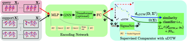
Figure 1: Supervised few-shot action recognition of the articulated human 3D body joints with the uncertainty-DTW (uDTW). Frames from a query and support sequences are split into short-term temporal blocks $\mathbf{X}_{1},...,\mathbf{X}_{\tau}$ and $\mathbf{X}^{\prime}_{1},...,\mathbf{X}^{\prime}_{\tau^{\prime}}$ of length $M$ given stride $S$. We pass all skeleton coordinates via Encoding Network to obtain feature tensors $\bm{\Psi}$ and $\bm{\Psi}^{\prime}$, which are directed to the Supervised Comparator with uDTW. For each query-support pair $(\bm{\Psi}_{n},\bm{\Psi}^{\prime}_{n})$, uDTW computes the base-distance matrix $\mathbf{D}_{n}$ reweighted by uncertainty $\bm{\Sigma}^{\dagger}_{n}$ to compare $\tau\!\times\!\tau^{\prime}$ blocks, and SigmaNet generates underlying block-wise uncertainty parameters $\bm{\Sigma}_{n}$. uDTW finds the warping path with the smallest distance, and returns its $\Omega_{n}$ penalty (uncertainty aggregated along the path).

However, the path distance $\left\langle{\bm{\Pi}},\bm{D}(\bm{\Psi},\bm{\Psi}^{\prime})\right\rangle$ of path ${\bm{\Pi}}$ ignores the observation uncertainty of frame-wise feature representations by simply relying on the Euclidean distances stored in $\bm{D}$. Thus, we resort to the notion of the so-called aleatoric uncertainty known from a non-exhaustive list of works about uncertainty [28, 18, 15, 14, 17].

Specifically, to capture the aleatoric uncertainty of the Euclidean distance (or regression, etc.), one should tune the observation noise parameter of sequences. Instead of the homoscedastic model (constant observation noise), we opt for the so-called heteroscedastic aleatoric uncertainty model (the observation noise may vary with each frame/sequence). To this end, we model each path distance by the product of likelihoods of Normal distributions (we also investigate other distributions in Appendix Sec. 0.F).

where $\odot$ is the Hadamard product, $\bm{\Sigma}^{{\dagger}}(\bm{\Psi},\bm{\Psi}^{\prime})$ is the element-wise inverse of matrix $\bm{\Sigma}\!\in\!\mathbb{R}_{+}^{\tau\times\tau^{\prime}}\!\!\equiv\![\sigma^{2}(\bm{\psi}_{m},\bm{\psi}^{\prime}_{n})]_{(m,n)\in\mathcal{I}_{\tau}\times\mathcal{I}_{\tau^{\prime}}}$ which contains pair-wise variances between all possible pairings of frame-wise feature representations from sequences $\bm{\Psi}$ and $\bm{\Psi}^{\prime}$. $\operatorname*{SoftMin_{\gamma}}(\bm{\alpha})\!=\!\sum_{i}\alpha_{i}\frac{\exp(-(\alpha_{i}\!-\!\mu_{\alpha})/\gamma)}{\sum_{j}\exp(-(\alpha_{j}\!-\!\mu_{\alpha})/\gamma)}$ with $\mu_{\alpha}$ (the mean over coefficients of $\bm{\alpha}$) subtracted from each coefficient $\alpha_{i}$ to attain stability of the softmax (into which we feed $(\alpha_{i}\!-\!\mu_{\alpha})$). Moreover, $\operatorname*{SoftMinSel_{\gamma}}(\bm{\alpha},\bm{\beta})\!=\!\sum_{i}\beta_{i}\frac{\exp(-(\alpha_{i}\!-\!\mu_{\alpha})/\gamma)}{\sum_{j}\exp(-(\alpha_{j}\!-\!\mu_{\alpha})/\gamma)}$ is a soft-selector returning $(\beta_{i^{*}}\!\!:i^{*}\!=\!\operatorname*{arg\,min}_{i}\alpha_{i})$ if $\gamma$ approaches zero.

Eq. (5) yields the uncertainty-weighted time warping distance $d^{2}_{\text{uDTW}}(\bm{D},\bm{\Sigma}^{{\dagger}})$ between sequences $\bm{\Psi}$ and $\bm{\Psi}^{\prime}$ because $\bm{D}$ and $\bm{\Sigma}^{{\dagger}}$ are both functions of $(\bm{\Psi},\bm{\Psi}^{\prime})$.

Eq. (LABEL:eq:unc_pen) provides the regularization penalty $\Omega(\bm{\Sigma})$ for sequences $\bm{\Psi}$ and $\bm{\Psi}^{\prime}$ (as $\bm{\Sigma}$ is a function of $(\bm{\Psi},\bm{\Psi}^{\prime})$) which is the aggregation of log-variances along the path with the smallest distance, i.e., path matrix $(({\bm{\Pi}}_{i^{*}}\!\in\!\{0,1\}^{\tau\times\tau^{\prime}}\!)\!\!:i^{*}\!=\!\operatorname*{arg\,min}_{k}w_{k})$ if $\gamma\!=\!0$, and vector $\bm{w}$ contains path-aggregated distances for all possible paths of the plan $\mathcal{A}_{\tau,\tau^{\prime}}$.

Contributions.

The celebrated DTW warps the matching path between a pair of sequences to recover the best matching distance under varying temporal within-class dynamics of each sequence. The recovered path, and the distance corresponding to that path, may be suboptimal if frame-wise (or block-wise) features contain noise (frames that are outliers, contain occlusions or large within-class object variations, etc.)

To this end, we propose several contributions:

1. We introduce the uncertainty-DTW, dubbed as uDTW, whose role is to take into account the uncertainty of in frame-wise (or block-wise) features by selecting the path which maximizes the Maximum Likelihood Estimation (MLE). The parameters (such as variance) of a distribution (i.e., the Normal distribution) are thus used within MLE (and uDTW) to model the uncertainty.

2. As pairs of sequences are often of different lengths, optimizing the free-form variable of variance is impossible. To that end, we equip each of our pipelines with SigmaNet, whose role is to take frames (or blocks) of sequences, and generate the variance end-to-end (the variance is parametrized by SigmaNet).

3. We provide several pipelines that utilize uDTW for (1) forecasting the evolution of time series, (2) estimating the Fréchet mean of time series, (3) supervised few-shot action recognition, and (4) unsupervised few-shot action recognition.

Notations.

$\mathcal{I}_{\tau}$ is the index set $\{1,2,...,\tau\}$. Concatenation of $\alpha_{i}$ into a vector $\bm{\alpha}$ is denoted by $[\alpha_{i}]_{i\in\mathcal{I}_{I}}$. Concatenation of $\alpha_{ij}$ into matrix $\mathbf{A}$ is denoted by $[\alpha_{ij}]_{(i,j)\in\mathcal{I}_{I}\times\mathcal{I}_{J}}$. Dot-product between two matrices equals the dot-product of vectorized ${\bm{\Pi}}$ and $\bm{D}$, that is $\left\langle{\bm{\Pi}},\bm{D}\right\rangle\!\equiv\!\left\langle\text{vec}({{\bm{\Pi}}}),\text{vec}(\bm{D})\right\rangle$. Mathcal symbols are sets, e.g., $\mathcal{A}$ is a transportation plan, capitalized bold symbols are matrices, e.g., $\bm{D}$ is the distance matrix, lowercase bold symbols are vectors, e.g., $\bm{w}$ contains weighted distances. Regular fonts are scalars.

(a) $\text{sDTW}_{\gamma=0.01}$

(b) $\text{sDTW}_{\gamma=0.1}$

(c) $\text{uDTW}_{\gamma=0.01}$

(d) $\text{uDTW}_{\gamma=0.1}$

(e) uDTW uncert.

Figure 2: Plots (a)-(d) show paths of sDTW and uDTW (in white) for a pair of sequences. We power-normalized pixels of plots (by the power of 0.1) to see also darker paths better. With higher $\gamma$ that controls softness, in (b) & (d) more paths become ‘active’ (fuzzy effect). In (c), uDTW has two possible routes vs. sDTW (a) due to uncertainty modeling. In (e), we visualise uncertainty $\bm{\Sigma}$. We binarize plot (c) and multiply it by the $\bm{\Sigma}$ to display uncertainty values on the path (white pixels = high uncertainty). The middle of the main path is deemed uncertain, which explains why an additional path merges in that region with the main path. See also the histogram of values of $\bm{\Sigma}$.

1.1 Similarity learning with uDTW

In further chapters, based on the distance in Eq. (5) and the regularization term in Eq. (LABEL:eq:unc_pen), we define specific loss functions for several problems such as forecasting the evolution of time series, clustering time series or even matching sequence pairs in few-shot action recognition. Below is an example of a generic similarity learning loss:

$$\operatorname*{arg\,min}_{\mathcal{P}}\sum_{n}\ell\left(d^{2}_{\text{uDTW}}(\bm{D}(\bm{\Psi}_{n},\bm{\Psi}^{\prime}_{n}),\bm{\Sigma}^{{\dagger}}(\bm{\Psi}_{n},\bm{\Psi}^{\prime}_{n})),\,\delta_{n}\right)+\beta\Omega(\bm{\Sigma}(\bm{\Psi}_{n},\bm{\Psi}^{\prime}_{n})),$$ (7)

or

$$\operatorname*{arg\,min}_{\mathcal{P},\bm{\Sigma}>0}\sum_{n}\ell\left(d^{2}_{\text{uDTW}}(\bm{D}(\bm{\Psi}_{n},\bm{\Psi}^{\prime}_{n}),\bm{\Sigma}^{{\dagger}}),\,\delta_{n}\right)+\beta\Omega(\bm{\Sigma}),$$ (8)

where $\bm{\Psi}_{n}\!=\!f(\mathbf{X}_{n};\mathcal{P})$ and $\bm{\Psi}^{\prime}_{n}\!=\!f(\mathbf{X}^{\prime}_{n};\mathcal{P})$ are obtained from some backbone encoder $f(\cdot;\mathcal{P})$ with parameters $\mathcal{P}$ and $(\mathbf{X}_{n},\mathbf{X}^{\prime}_{n})\!\in\!\mathcal{X}$ is a sequence pair to compare with the similarity label $\delta_{n}\!\in\!\{0,1\}$ (where $\delta_{n}\!=\!0$ if $y_{n}\!=\!y^{\prime}_{n}$ and $\delta_{n}\!=\!1$ otherwise), $(y_{n},y^{\prime}_{n})$ is a pair of class labels for $(\bm{\Psi}_{n},\bm{\Psi}^{\prime}_{n})$, and $\beta\!\geq\!0$ controls the penalty for high matching uncertainty. Figure 2 illustrates the impact of uncertainty on uDTW.

1.2 Derivation of uDTW

We proceed by modeling an arbitrary path ${\bm{\Pi}}_{i}$ from the transportation plan of $\mathcal{A}_{\tau,\tau^{\prime}}$ as the following Maximum Likelihood Estimation (MLE) problem:

$$\operatorname*{arg\,max}\limits_{\{\sigma_{mn}\}_{(m,n)\in{\bm{\Pi}}_{i}}}\prod_{(m,n)\in{\bm{\Pi}}_{i}}p(\|\bm{\psi}_{m}\!-\!\bm{\psi}^{\prime}_{n}\|,\sigma^{2}_{mn}),$$ (13)

where $p$ may be some arbitrary distribution, $\sigma$ are distribution parameters, and $\|\cdot\|$ is an arbitrary norm. For the Normal distribution $\mathcal{N}$ which relies on the squared Euclidean distance $\|\cdot\|_{2}^{2}$, we have:

$$\operatorname*{arg\,max}\limits_{\{\sigma_{mn}\}_{(m,n)\in{\bm{\Pi}}_{i}}}\prod_{(m,n)\in{\bm{\Pi}}_{i}}\mathcal{N}(\bm{\psi}_{m};\bm{\psi}^{\prime}_{n},\sigma^{2}_{mn})$$ (14)

$$\quad=\operatorname*{arg\,max}\limits_{\{\sigma_{mn}\}_{(m,n)\in{\bm{\Pi}}_{i}}}\log\prod_{(m,n)\in{\bm{\Pi}}_{i}}\frac{1}{(2\pi)^{\frac{d^{\prime}}{2}}\sigma^{d^{\prime}}}\exp\Big{(}\!-\frac{\|\bm{\psi}_{m}\!-\!\bm{\psi}^{\prime}_{n}\|_{2}^{2}}{\sigma^{2}_{mn}}\Big{)}$$ (15)

$$\quad=\operatorname*{arg\,max}\limits_{\{\sigma_{mn}\}_{(m,n)\in{\bm{\Pi}}_{i}}}\sum_{(m,n)\in{\bm{\Pi}}_{i}}-\frac{d^{\prime}}{2}\log(2\pi)-d^{\prime}\log(\sigma)-\frac{\|\bm{\psi}_{m}\!-\!\bm{\psi}^{\prime}_{n}\|_{2}^{2}}{\sigma^{2}_{mn}}$$ (16)

$$\quad=\operatorname*{arg\,min}\limits_{\{\sigma_{mn}\}_{(m,n)\in{\bm{\Pi}}_{i}}}\sum_{(m,n)\in{\bm{\Pi}}_{i}}d^{\prime}\log(\sigma)+\frac{\|\bm{\psi}_{m}\!-\!\bm{\psi}^{\prime}_{n}\|_{2}^{2}}{\sigma^{2}_{mn}},$$ (17)

where $d^{\prime}$ is the length of feature vectors $\bm{\psi}$. Having recovered uncertainty parameters ${\{\sigma_{mn}\}_{(m,n)\in{\bm{\Pi}}_{i}}}$, we obtain a combination of penalty terms and reweighted squared Euclidean distances:

$$\beta\Omega_{{\bm{\Pi}}_{i}}+d^{2}_{{\bm{\Pi}}_{i}}\!=\!\sum_{(m,n)\in{\bm{\Pi}}_{i}}\beta\log(\sigma_{mn})+\frac{\|\bm{\psi}_{m}\!-\!\bm{\psi}^{\prime}_{n}\|_{2}^{2}}{\sigma^{2}_{mn}},$$ (18)

where $\beta\!\geq\!0$ (generally $\beta\!\neq\!d^{\prime}$) adjusts the penalty for large uncertainty. Separating the uncertainty penalty $\log(\sigma_{mn})$ from the uncertainty-weighted distance (both aggregated along path ${\bm{\Pi}}_{i}$) yields:

$$\left\{\begin{array}[]{l}d^{2}_{{\bm{\Pi}}_{i}}\!=\!\left\langle{\bm{\Pi}}_{i},\bm{D}(\bm{\Psi},\bm{\Psi}^{\prime})\!\odot\!\bm{\Sigma}^{{\dagger}}\right\rangle\\ \Omega_{{\bm{\Pi}}_{i}}\!=\!\left\langle{\bm{\Pi}}_{i},\log\!\bm{\Sigma}\right\rangle,\end{array}\right.$$ (21)

where $\bm{D}\!\in\!\mathbb{R}_{+}^{\tau\times\tau^{\prime}}\!\!\equiv\!\big{[}\frac{d^{2}_{2}(\bm{\psi}_{m},\bm{\psi}^{\prime}_{n})}{\sigma^{2}_{mn}}\big{]}_{(m,n)\in\mathcal{I}_{\tau}\times\mathcal{I}_{\tau^{\prime}}}$ and $\bm{\Sigma}\!\in\!\mathbb{R}_{+}^{\tau\times\tau^{\prime}}\!\!\equiv\![\sigma^{2}_{mn}]_{(m,n)\in\mathcal{I}_{\tau}\times\mathcal{I}_{\tau^{\prime}}}$. Derivations for other distributions, i.e., Laplace or Cauchy, follow the same reasoning.

2 Related Work

Different flavors of Dynamic Time Warping. DTW [6], which seeks a minimum cost alignment between time series is computed by dynamic programming in quadratic time, is not differentiable and is known to get trapped in bad local minima. In contrast, soft-DTW (sDTW) [7] addresses the above issues by replacing the minimum over alignments with a soft minimum, which has the effect of inducing a ‘likelihood’ field over all possible alignments. However, sDTW has been successfully applied in many computer vision tasks including audio/music score alignment [31], action recognition [39, 4], and end-to-end differentiable text-to-speech synthesis [10]. Despite its successes, sDTW has some limitations: (i) it can be negative when used as a loss (ii) it may still get trapped in bad local minima. Thus, soft-DTW divergences (sDTW div.) [3], inspired by sDTW, attempts to overcome such issues.

Other approaches inspired by DTW have been used to improve the inference or adapt to modified or additional constraints, i.e., OPT [38] and OWDA [40] treat the alignment as the optimal transport problem with temporal regularization. TAP [39] directly predicts the alignment through a lightweight CNN, thus is does not follow a principled transportation plan, and is not guaranteed to find a minimum cost path.

Our uDTW differs from these methods in that the transportation plan is executed under the uncertainty estimation, thus various feature-level noises and outliers are less likely to lead to the selection of a sub-optimal cost path.

Alignment-based time series problems. Distance between sequences plays an important role in time series retrieval [40], forecasting [7, 3], classification [7, 3, 9, 49], clustering [12, 35], etc. Various temporal nuisance noises such as initial states, different sampling rates, local distortions, and execution speeds make the measurement of distance between sequences difficult. To tackle these issues, typical feature-based methods use RNNs to encode sequences and measure the distance between corresponding features [34]. Other existing methods [43, 45, 20] either encode each sequence into features that are invariant to temporal variations [1, 26] or adopt alignment for temporal correspondence calibration [38]. However, none of these methods is modeling the aleatoric uncertainty. As we model it along the time warping path, the observation noise may vary with each frame or block.

Few-shot action recognition. Most existing few-shot action recognition methods [44, 47, 46] follow the metric learning paradigm. Signal Level Deep Metric Learning [30] and Skeleton-DML [29] one-shot FSL approaches encode signals into images, extract features using a deep residual CNN and apply multi-similarity miner losses. TAEN [2] and FAN [41] encode actions into representations and apply vector-wise metrics.

Most methods identify the importance of temporal alignment for handling the non-linear temporal variations, and various alignment-based models are proposed to compare the sequence pairs, e.g., permutation-invariant spatial-temporal attention reweighted distance in ARN [50], a variant of DTW used in OTAM [4], temporal attentive relation network [32], a two-stage temporal alignment network (TA2N) [22], a temporal CrossTransformer [33], a learnable sequence matching distance called TAP [39].

In all cases, temporal alignment is a well-recognized tool, however lacking the uncertainty modeling, which impacts the quality of alignment. Such a gap in the literature inspires our work on uncertainty-DTW.

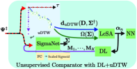
(a)

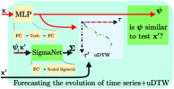
(b)

Figure 3: In (a) is the unsupervised comparator for unsupervised few-shot action recognition. The unsupervised head is wired with the Encoding Network from Figure 1, and trained from scratch without labels. In (b) is the pipeline for forecasting the evolution of time series (a.k.a. multistep-ahead prediction).

3 Pipeline Formulations

Below we provide our several pipeline formulations for which uDTW is used as an indispensable component embedded with the goal of measuring the distance for warped paths under uncertainty.

3.1 Few-shot Action Recognition

For both supervised and unsupervised few-shot pipelines, we employ the Encoder Network (EN) and the Supervised Comparator (similarity learning) as in Figure 1, or Unupervised Comparator (based on dictionary learning) as in Figure 3(a).

Encoding Network (EN).

Our EN contains a simple 3-layer MLP unit (FC, ReLU, FC, ReLU, Dropout, FC), GNN, with transformer [11] and FC. The MLP unit takes $M$ neighboring frames, each with $J$ skeleton body joints given by Cartesian coordinates $(x,y,z)$, forming one temporal block. In total, depending on stride $S$, we obtain some $\tau$ temporal blocks (each block captures the short temporal dependency), whereas the long temporal dependency will be modeled by uDTW. Each temporal block is encoded by the MLP into a $d\!\times\!J$ dimensional feature map. Subsequently, query feature maps of size $\tau$ and support feature maps of size $\tau^{\prime}$ are forwarded to a simple linear GNN model, and transformer, and an FC layer, which returns $\bm{\Psi}\!\in\!\mathbb{R}^{d^{\prime}\times\tau}$ query feature maps and $\bm{\Psi}^{\prime}\!\in\!\mathbb{R}^{d^{\prime}\times\tau^{\prime}}\!$ support feature maps. Such encoded feature maps are passed to the Supervised Comparator with uDTW.

Let support maps $\bm{\Psi}^{\prime}\!\equiv\![f(\bm{X}^{\prime}_{1};\mathcal{P}),...,f(\bm{X}^{\prime}_{\tau^{\prime}};\mathcal{P})]\!\in\!\mathbb{R}^{d^{\prime}\times\tau^{\prime}}\!$ and query maps $\bm{\Psi}\!\equiv\![f(\bm{X}_{1};\mathcal{P}),...,f(\bm{X}_{\tau};\mathcal{P})]\!\in\!\mathbb{R}^{d^{\prime}\times\tau}$ for query and support frames per block $\mathbf{X},\mathbf{X}^{\prime}\!\in\!\mathbb{R}^{3\times J\times M}$. Define $f(\mathbf{X};\mathcal{P})\!=\!\text{FC}(\text{Transf}(\text{S\textsuperscript{2}GC}(\text{MLP}(\mathbf{X};\mathcal{P}_{MLP});\mathcal{P}_{S^{2}GC});$ $\mathcal{P}_{Transf});\mathcal{P}_{FC})$ where $\mathcal{P}\!\equiv\![\mathcal{P}_{MLP},\mathcal{P}_{S^{2}GC},\mathcal{P}_{Transf},\mathcal{P}_{FC},\mathcal{P}_{SN}]$ is the set of parameters of EN, where $\mathcal{P}_{SN}$ are parameters of SigmaNet, and S²GC is a Simple Spectral Graph Convolution (S²GC) [51] whose details are in Sec. 0.H.3 of the Appendix.

Supervised Few-shot Action Recognition.

For the $N$-way $Z$-shot problem, we have one query feature map and $N\!\times\!Z$ support feature maps per episode. We form a mini-batch containing $B$ episodes. We have query feature maps $\{\bm{\Psi}_{b}\}_{b\in\mathcal{I}_{B}}$ and support feature maps $\{\bm{\Psi}^{\prime}_{b,n,z}\}_{b\in\mathcal{I}_{B},n\in\mathcal{I}_{N},z\in\mathcal{I}_{Z}}$. Moreover, $\bm{\Psi}_{b}$ and $\bm{\Psi}^{\prime}_{b,1,:}$ share the same class (drawn from $N$ classes per episode), forming the subset $C^{\ddagger}\equiv\{c_{1},...,c_{N}\}\subset\mathcal{I}_{C}\equiv\mathcal{C}$. To be precise, labels $y(\bm{\Psi}_{b})\!=\!y(\bm{\Psi}^{\prime}_{b,1,z}),\forall b\!\in\!\mathcal{I}_{B},z\!\in\!\mathcal{I}_{Z}$ while $y(\bm{\Psi}_{b})\!\neq\!y(\bm{\Psi}^{\prime}_{b,n,z}),\forall b\!\in\!\mathcal{I}_{B},n\!\in\!\mathcal{I}_{N}\!\setminus\!\{1\},z\!\in\!\mathcal{I}_{Z}$. Thus the similarity label $\delta_{1}\!=\!0$, whereas $\delta_{n\neq 1}\!=1\!$. Note that the selection of $C^{\ddagger}$ per episode is random. For the $N$-way $Z$-shot protocol, the Supervised Comparator is minimized w.r.t. $\mathcal{P}$ ($\bm{\Psi}_{b}$ and $\bm{\Psi}^{\prime}$ depend on $\mathcal{P}$) as:

$$\operatorname*{arg\,min}_{\mathcal{P}}\sum_{b\in\mathcal{I}_{B}}\sum_{n\in\mathcal{I}_{N}}\sum_{z\in\mathcal{I}_{Z}}\left(d^{2}_{\text{uDTW}^{\bullet}}(\bm{\Psi}_{b},\bm{\Psi}^{\prime}_{b,n,z})-\delta_{n}\right)^{2}\!+\beta\Omega_{\bullet}(\bm{\Psi}_{b},\bm{\Psi}^{\prime}_{b,n,z}).$$ (22)

Unsupervised Few-shot Action Recognition.

Below we propose a very simple unsupervised variant with so-called Unsupervised Comparator. The key idea is that with uDTW, invariant to local temporal speed changes can be used to learn a dictionary which, with some dictionary coding method should outperform at reconstructing the sequences. This means we can learn an unsupervised comparator by projecting sequences onto the dictionary space. To this end, let the protocol remain as for the supervised few-shot learning with the exception that class labels are not used during training, and only support images in testing are labeled for sake of evaluation the accuracy by deciding which support representation each query is the closest to in the nearest neighbor sense.

Firstly, in each training episode, we combine the query sequences $\bm{\Psi}_{b}$ with the support sequences $\bm{\Psi}^{\prime}_{b,n,z}$ into episode sequences denoted as $\bm{\Psi}^{\ddagger}_{b,n}$ where $b\!\in\!\mathcal{I}_{B}$ enumerates over $B$ episodes, and $n\!\in\!\mathcal{I}_{(N\cdot Z+1)}$. For the feature coding, we use Locality-constrained Soft Assignment (LCSA) [25, 19, 21] and a simple dictionary update based on the least squares computation.

For each episode $b\!\in\!\mathcal{I}_{B}$, we iterate over the following three steps:

1. The LCSA coding step which expresses each $\bm{\Psi}^{\ddagger}_{b,n}$ as $\bm{\alpha}_{b,n}\!\in\!\mathbb{R}_{+}^{K}$ that assign $\bm{\Psi}^{\ddagger}_{b,n}$ into a dictionary with $K$ sequences $\bm{M}_{1},...,\bm{M}_{K}\!\in\!\mathbb{R}^{d^{\prime}\times\tau^{\prime}}$ (dictionary anchors):

   $$\!\!\!\!\forall_{k,n},\;\alpha_{k,b,n}\!=\!\left\{\begin{array}[]{l}\frac{\exp\big{(}-\frac{1}{\gamma^{\prime}}d^{2}_{\text{uDTW}^{\bullet}}\big{(}\bm{\Psi}^{\ddagger}_{b,n},\bm{M}_{k}\big{)}\big{)}}{\!\!\!\!\sum\limits_{l\in\mathcal{M}(\bm{\Psi}^{\ddagger}_{b,n};K^{\prime})}\!\!\!\!\exp\big{(}-\frac{1}{\gamma^{\prime}}d^{2}_{\text{uDTW}^{\bullet}}\big{(}\bm{\Psi}^{\ddagger}_{b,n},\bm{M}_{l}\big{)}\big{)}}\quad\text{if}\;\;\bm{M}_{k}\!\in\!\mathcal{M}\big{(}\bm{\Psi}^{\ddagger}_{b,n};K^{\prime}\big{)},\\ 0\qquad\qquad\qquad\qquad\qquad\text{otherwise},\end{array}\right.$$ (25)

   where $0\!<\!K^{\prime}\!\leq\!K$ is a subset size for $K^{\prime}$ nearest anchors of $\bm{\Psi}^{\ddagger}_{b,n}$ retrieved by operation $\mathcal{M}(\bm{\Psi}^{\ddagger}_{b,n};K^{\prime})$ (based on uDTW) from $\bm{M}_{1},...,\bm{M}_{K}$, $\tau^{\prime}$ is set to the mean of $\tau$ (over training set), and $\gamma^{\prime}\!=\!0.7$ is a so-called smoothing factor;

2. The dictionary update step updates $\bm{M}_{1},...,\bm{M}_{K}$ given $\bm{\alpha}_{b,n}$ from Eq. (LABEL:eq:lcsa):

   for i=1,...,dict_iter:

   $$\qquad\forall_{k},\;\bm{M}_{k}:=\bm{M}_{k}\!-\!\lambda_{\text{DL}}\!\!\sum_{n=1}^{N\!\cdot\!Z+1}\!\!\nabla_{\bm{M}_{k}}d^{2}_{\text{uDTW}^{\bullet}}\Big{(}\bm{\Psi}^{\ddagger}_{b,n},\sum_{l=1}^{K}\alpha_{l,b,n}\bm{M}_{l}\Big{)},$$ (27)

   where dict_iter is set to 10 and $\lambda_{\text{DL}}\!=\!0.001$;

3. The main loss for the Feature Encoder update step is given as ($\lambda_{\text{EN}}\!=\!0.001$):

   $$\mathcal{P}:=\mathcal{P}\!-\!\lambda_{\text{EN}}\!\!\sum_{n=1}^{N\!\cdot\!Z+1}\!\!\nabla_{\mathcal{P}}d^{2}_{\text{uDTW}^{\bullet}}\Big{(}\bm{\Psi}^{\ddagger}_{b,n},\bm{M}^{\prime}\Big{)}\!+\!\beta\Omega_{\bullet}\Big{(}\bm{\Psi}^{\ddagger}_{b,n},\bm{M}^{\prime}\Big{)},$$ (28)

   $$\qquad\;\text{where}\;\;\bm{M}^{\prime}\!=\!\sum_{l=1}^{K}\alpha_{l,b,n}\bm{M}_{l}.$$

During testing, we use the learnt dictionary, pass new support and query sequences via Eq. (LABEL:eq:lcsa) and obtain $\bm{\alpha}$ codes. Subsequently, we compare the LCSA code of the query sequence with LCSA codes of support sequences via the histogram intersection kernel. The closest match in the support set determines the test label of the query sequence.

3.2 Time Series Forecasting and Classification

One of key applications of DTW and sDTW is learning with time series, including forecasting the evolution of time series as in Figure 3(b) and time series classification.

Forecasting the Evolution of Time Series.

Let $\mathbf{x}\!\in\!\mathbb{R}^{t}$ and $\mathbf{x}^{\prime}\!\in\!\mathbb{R}^{\tau-t}$ be the training and testing parts of one time series corresponding to timesteps $1,...,t$ and $t\!+\!1,...,\tau$, respectively. The goal is to learn encoder $f(\mathbf{x};\mathcal{P})\!\in\!\mathbb{R}^{\tau-t}$ which will be able to take $\mathbf{x}$ as input, learn to translate it to $\mathbf{x}^{\prime}$. Figure 3(b) show the full pipeline. We took the Encoding Network from the original soft-DTW pipeline [7]. Our training objective is:

$$\operatorname*{arg\,min}_{\mathcal{P}}\sum_{n\in\mathcal{I}_{N}}d^{2}_{\text{uDTW}^{\bullet}}(\bm{\psi}_{n},\mathbf{x}^{\prime}_{n})\!+\beta\Omega_{\bullet}(\bm{\psi}_{n},\mathbf{x}^{\prime}_{n}),$$ (29)

where $\bm{\psi}\!=\!f(\mathbf{x};\mathcal{P})$ and $N$ is the number of training time series, $\mathcal{P}\!\equiv\![\mathcal{P}_{MLP},\mathcal{P}_{SN}]$ is the set of parameters of EN and SigmaNet. In order to obtain $\bm{\Sigma}$, vectors $\bm{\psi}$ and $\mathbf{x}^{\prime}$ are passed via SigmaNet. After training, at the test time, for a previously unseen testing sample $\mathbf{x}$, $f(\cdot)$ has to predict the remaining part of the time series given by $\mathbf{x}^{\prime}$.

Time Series Classification.

Below we follow the setting for this classical task according to the original soft-DTW paper [7], and define the nearest centroid classifier. We estimate the Fréchet mean of training time series of each class separately. We do not use any Encoding Network but the raw features. Let $\mathbf{x}\!\in\!\mathbb{R}^{\tau}$ be training samples and $\bm{\mu}\!\in\!\mathbb{R}^{\tau^{\prime}}$ be class prototypes ($\tau^{\prime}$ is set to average of $\tau$ across all classes). We have:

$$\forall_{c},\;\operatorname*{arg\,min}_{\mathcal{P}}\sum_{n\in\mathcal{I}_{N_{c}}}d^{2}_{\text{uDTW}^{\bullet}}(\mathbf{x}_{n},\bm{\mu}_{c})\!+\beta\Omega_{\bullet}(\mathbf{x}_{n},\bm{\mu}_{c}),$$ (30)

where $N_{c}$ is the number of samples for class $c\!\in\!\mathcal{I}_{C}$ and $\mathcal{P}\!\equiv\![\mathcal{P}_{SN},\bm{\mu}_{c}]$. During testing, we apply $\operatorname*{arg\,min}_{c\in\mathcal{I}_{C}}d^{2}_{\text{uDTW}^{\bullet}}(\mathbf{x},\bm{\mu}_{c})\!+\beta\Omega_{\bullet}(\mathbf{x},\bm{\mu}_{c})$ for $\mathbf{x}$ to find its nearest neighbor and label it. The variances of $\mathbf{x}$ are recovered through SigmaNet while variances of $\bm{\mu}_{c}$ were obtained during training (adding both yields $\bm{\Sigma}$ of testing sample). As in soft-DTW paper [7], we use uDTW to directly find the nearest neighbor of $\mathbf{x}$ across training samples to label $\mathbf{x}$ (for uncertainty, we use SigmaNet from the nearest centroid task).

4 Experiments

Below we apply uDTW in several scenarios such as (i) forecasting the evolution of time series, (ii) clustering/classifying time series, (iii) supervised few-shot action recognition, and (iv) unsupervised few-shot action recognition.

Datasets. The following datasets are used in our experiments:

1. UCR archive [8] is a dataset for time series classification archive. This dataset contains a wide variety of fields (astronomy, geology, medical imaging) and lengths, and can be used for time series classification/clustering and forecasting tasks.

2. NTU RGB+D (NTU-60) [36] contains 56,880 video sequences and over 4 million frames. NTU-60 has variable sequence lengths and high intra-class variations.

3. NTU RGB+D 120 (NTU-120) [24], an extension of NTU-60, contains 120 action classes (daily/health-related), and 114,480 RGB+D video samples captured with 106 distinct human subjects from 155 different camera viewpoints.

4. Kinetics [16] is a large-scale collection of 650,000 video clips that cover 400/600/700 human action classes. It includes human-object interactions such as playing instruments, as well as human-human interactions such as shaking hands and hugging. We follow approach [48] and use the estimated joint locations in the pixel coordinate system as the input to our pipeline. As OpenPose produces the 2D body joint coordinates and Kinetics-400 does not offer multiview or depth data, we use a network of Martinez et al. [27] pre-trained on Human3.6M [5], combined with the 2D OpenPose output to estimate 3D coordinates from 2D coordinates. The 2D OpenPose and the latter network give us $(x,y)$ and $z$ coordinates, respectively.

4.1 Fréchet Mean of Time Series

Below, we visually inspect the Fréchet mean for the Euclidean, sDTW and our uDTW distance, respectively.

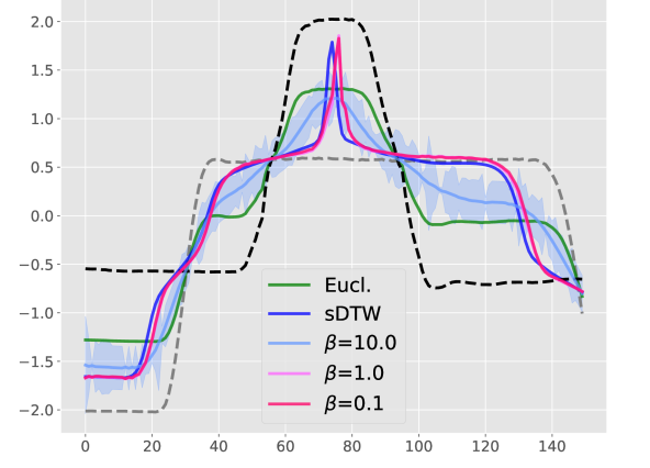
(a) $\beta$ (where $\lambda\!=\!1$)

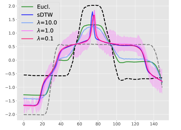
(b) $\lambda$ (where $\beta\!=\!10$)

Figure 4: Interpolation between two time series (grey and black dashed lines) on the Gun Point dataset. We compute the barycenter by solving $\operatorname*{arg\,min}\limits_{\bm{\mu},\bm{\sigma}_{\mu}}\sum_{n=1}^{2}d^{2}_{\text{uDTW}}\big{(}\bm{D},\bm{\Sigma}^{\dagger}\big{)}+\beta\Omega\big{(}\bm{\Sigma}\big{)}+\lambda\Omega^{\prime}\big{(}\bm{\Sigma}\big{)}$ where $\bm{D}\!=\!(\mathbf{x}_{n}\mathbf{1}^{\top}\!-\!\mathbf{1}\bm{\mu}^{\top})^{2}$ and $\bm{\Sigma}\!=\!\mathbf{1}\mathbf{1}^{\top}\!\!+\!\mathbf{1}\bm{\sigma}_{\mu}^{\top}$ where $\mathbf{x}_{n}$ is the given $n$-th time series. $\beta\!\geq\!0$ controls the penalty for high matching uncertainty, $\Omega^{\prime}$ is defined as in Eq. (LABEL:eq:unc_pen) but element-wise $\log\!\bm{\Sigma}$ is replaced by element-wise $(\bm{\Sigma}\!-\!1)^{2}$ so that $\lambda\!\geq\!0$ favours uncertainty to remain close to one. $\beta$ and $\lambda$ control the uncertainty estimation and yield different barycenters than the Euclidean (green color) and sDTW (blue color) distances. As $\Omega$ and $\Omega^{\prime}$ act similar, we only use $\Omega$ in our experiments.

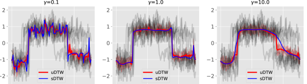
(a) CBF

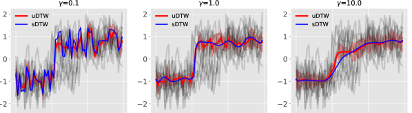
(b) Synthetic Control

Figure 5: Comparison of barycenter based on sDTW or uDTW on CBF and Synthetic Control. We visualize uncertainty around the barycenters in red color for uDTW. Our uDTW generates reasonable barycenters even when higher $\gamma$ values are used, e.g., $\gamma\!=\!10.0$. Higher $\gamma$ value leads to smooth barycenter but introducing higher uncertainty.

Experimental setup.

We follow the protocol of soft-DTW paper [7]. For each dataset in UCR, we choose a class at random, pick 10 time series from the selected class to compute its barycenter. We use L-BFGS [23] to minimise the proposed uDTW barycenter objective. We set the maximum number of iterations to 100.

Qualitative results.

We first perform averaging between two time series (Figure 4). We notice that averaging under the uDTW yields substantially different results than those obtained with the Euclidean and sDTW geometry.

Figure 5 shows the barycenters obtained using sDTW and our uDTW. We observe that our uDTW yields more reasonable barycenters than sDTW even when large $\gamma$ are used, e.g., for $\gamma\!=\!10$ (right column of plots in Figure 5), the change points of red curve look sharper. We also notice that both uDTW and sDTW with low smoothing parameter $\gamma\!=\!0.1$ can get stuck in some bad local minima, but our uDTW has fewer sharp peaks compared with sDTW (barycenters of uDTW are improved by the uncertainty measure). Moreover, higher $\gamma$ values smooth the barycenter but introducing higher uncertainty (see uncertainty visualization around the barycenters by comparing, e.g., $\gamma\!=\!0.1$ vs. $\gamma\!=\!10.0$). With $\gamma\!=\!1$, the barycenters of sDTW and uDTW match well with the time series. More visualizations can be found in Appendix Sec. 0.D.

4.2 Classification of Time Series

In this section, we devise the nearest neighbor and nearest centroid classifiers [13] with uDTW, as detailed in Section 3. For the $K$-nearest neighbor classifier, we used softmax for the final decision. See Appendix Sec. 0.H.4 for details.

Experimental setup.

We use 50% of the data for training, 25% for validation and 25% for testing. We report $K=$ 1, 2 and 3 for the nearest neighbor classifier.

Quantitative results.

Table 1 shows a comparison of our uDTW versus Euclidean, DTW, sDTW, and sDTW div. Unsurprisingly, the use of uDTW for barycenter computation improves the accuracy of the nearest centroid classifier, and it outperforms sDTW div. by $\sim$ 2%. Moreover, uDTW boosts results for the nearest neighbor classifier given $K$=1, 2 and 3 by 1.4%, 1.7% and 3.2%, respectively, compared to sDTW div.

Table 1: Classification accuracy (mean$\pm$std) on UCR archive by the nearest neighbor and the nearest centroid classifiers. In the column we indicate which distance was used for computing the class prototypes. $K$ is the number of nearest neighbors in this context.

	Nearest neighbor			Nearest centroid
	$K=1$	$K=3$	$K=5$
Euclidean	71.2$\pm$17.5	72.3$\pm$18.1	73.0$\pm$16.7	61.3$\pm$20.1
DTW [6]	74.2$\pm$16.6	75.0$\pm$17.0	75.4$\pm$15.8	65.9$\pm$18.8
sDTW [7]	76.2$\pm$16.6	77.2$\pm$15.9	78.0$\pm$16.5	70.5$\pm$17.6
sDTW div. [3]	78.6$\pm$16.2	79.5$\pm$16.7	80.1$\pm$16.5​​	70.9$\pm$17.8
uDTW	80.0$\pm$15.0	81.2$\pm$17.8	83.3$\pm$16.2	72.2$\pm$16.0

4.3 Forecasting the Evolution of Time Series

Experimental setup. We use the training and test sets pre-defined in the UCR archive. For both training and test, we use the first 60% of timesteps of series as input and the remaining 40% as output, ignoring the class information.

Qualitative results.

The visualization of the predictions are given in Figure 6. Although the predictions under the sDTW and uDTW losses sometimes agree with each other, they can be visibly different. Predictions under uDTW can confidently predict the abrupt and sharp changes. More visualizations can be found in Appendix Sec. 0.E.

Quantitative results.

We also provide quantitive results to validate the effectiveness of uDTW. We use ECG5000 dataset from the UCR archive which is composed of 5000 electrocardiograms (ECG) (500 for training and 4500 for testing) of length 140. To better evaluate the predictions, we use 2 different metrics (i) MSE for the predicted errors of each time step (ii) DTW, sDTW div. and uDTW for comparing the ‘shape’ of time series. We use such shape metrics for evaluation as the length of time series generally varies, and the MSE metric may lead to biased results which ignore the shape trend of time series. We then use the Student’s $t$-test (with significance level 0.05) to highlight the best performance in each experiment (averaged over 100 runs). Table 2 shows that our uDTW achieves almost the best performance on both MSE and shape evaluation metrics (lower score is better).

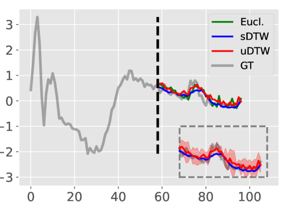
(a) ECG200

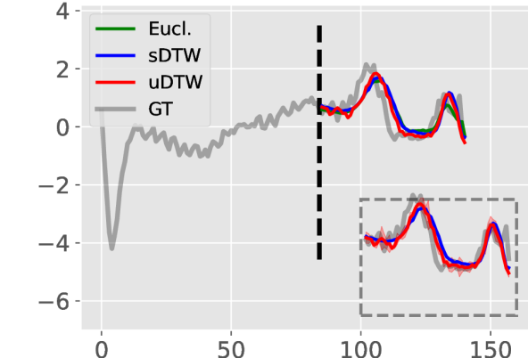
(b) ECG5000

Figure 6: Given the first part of a time series, we train 3 multi-layer perception (MLP) to predict the remaining part, we use the Euclidean, sDTW or uDTW distance per MLP. We use ECG200 and ECG5000 in UCR archive, and display the prediction obtained for the given test sample with either of these 3 distances and the ground truth (GT). Oftentimes, we observe that uDTW helps predict the sudden changes well.

Table 2: Time series forecasting results evaluated with MSE, DTW, sDTW div. and uDTW metrics on ECG5000, averaged over 100 runs (mean$\pm$std). Best method(s) are highlighted in bold using Student’s $t$-test. Column-wise distances indicate the distance used during training. Row-wise distances indicate the distance used to compare prediction with the groundtruth at the test time (lower values are better).

	MSE	DTW	sDTW div.	uDTW
Euclidean	32.1$\pm$1.62	20.0$\pm$0.18	15.3$\pm$0.16	14.4$\pm$0.18
sDTW [7]	38.6$\pm$6.30	17.2$\pm$0.80	22.6$\pm$3.59	32.1$\pm$2.25
sDTW div. [3]	24.6$\pm$1.37	38.9$\pm$5.33	20.0$\pm$2.44	15.4$\pm$1.62
uDTW	23.0$\pm$1.22	16.7$\pm$0.08	16.8$\pm$1.62	8.27$\pm$0.79

4.4 Few-shot Action Recognition

Below, we use uDTW as a distance in our objectives for few-shot action recognition (AR) tasks. We implement supervised and unsupervised pipelines (which is also novel).

Experimental setup.

For NTU-120, we follow the standard one-shot protocols [24]. Base on this protocol, we create a similar one-shot protocol for NTU-60, with 50/10 action classes used for training/testing respectively (see Appendix Sec. 0.C for details). We also evaluate the model on both 2D and 3D Kinetics-skeleton. We split the whole Kinetics-skeleton into 200 actions for training (the rest is used for testing). We choose Matching Nets (MatchNets) and Prototypical Net (ProtoNet) as baselines as these two models are very popular baselines, and we adapt these methods to skeleton-based action recognition. We reshape and resize each video block into 224$\times$224 color image, and pass this image into MatchNets and ProtoNet to learn the feature representation per video block. We compare uDTW vs. Euclidean, sDTW, sDTW div. and recent TAP.

Quantitative results.

Table 4, 4 and 5 show that our uDTW performs better than sDTW and sDTW div. on both supervised and unsupervised few-shot action recognition. On Kinetics-skeleton dataset, we gain 2.4% and 4.4% improvements on 3D skeletons for supervised and unsupervised settings. On supervised setting, we outperform TAP by $\sim$ 4% and 2% on NTU-60 and NTU-120 respectively. Moreover, we outperform sDTW by $\sim$ 2% and 3% on NTU-60 and NTU-120 for the unsupervised setting. More evaluations on few-shot action recognition are in Appendix Sec. 0.F.

Table 3: Evaluations on NTU-60.

#classes	10	20	30	40	50
	Supervised
MatchNets [42]	46.1	48.6	53.3	56.3	58.8
ProtoNet [37]	47.2	51.1	54.3	58.9	63.0
TAP [39]	54.2	57.3	61.7	64.7	68.3
Euclidean	38.5	42.2	45.1	48.3	50.9
sDTW [7]	53.7	56.2	60.0	63.9	67.8
sDTW div. [3]	54.0	57.3	62.1	65.7	69.0
uDTW	56.9	61.2	64.8	68.3	72.4
	Unsupervised
Euclidean	20.9	23.7	26.3	30.0	33.1
sDTW [7]	35.6	45.2	53.3	56.7	61.7
sDTW div. [3]	36.0	46.1	54.0	57.2	62.0
uDTW	37.0	48.3	55.3	58.0	63.3

Table 4: Evaluations on NTU-120.

#classes	20	40	60	80	100
	Supervised
MatchNets [42]	20.5	23.4	25.1	28.7	30.0
ProtoNet [37]	21.7	24.0	25.9	29.2	32.1
TAP [39]	31.2	37.7	40.9	44.5	47.3
Euclidean	18.7	21.3	24.9	27.5	30.0
sDTW [7]	30.3	37.2	39.7	44.0	46.8
sDTW div. [3]	30.8	38.1	40.0	44.7	47.3
uDTW	32.2	39.0	41.2	45.3	49.0
	Unsupervised
Euclidean	13.5	16.3	20.0	24.9	26.2
sDTW [7]	20.1	25.3	32.0	36.9	40.9
sDTW div. [3]	20.8	26.0	33.2	37.5	42.3
uDTW	22.7	28.3	35.9	39.4	44.0

Table 5: Evaluations on 2D and 3D Kinetics-skeleton.

	Supervised		Unsupervised
	2D	3D	2D	3D
Euclidean	21.2	23.1	12.7	13.3
TAP [39]	32.9	36.0	-	-
sDTW [7]	34.7	39.6	23.3	28.3
sDTW div. [3]	35.0	40.1	24.0	28.9
uDTW	35.5	42.0	25.9	32.7

5 Conclusions

We have introduced the uncertainty-DTW which handles the uncertainty estimation of frame- and/or block-wise features to improve the path warping of the celebrated soft-DTW. Our uDTW produces the uncertainty-weighted distance along the path and returns the regularization penalty aggregated along the path, which follows sound principles of classifier regularization. We have provided several pipelines for time series forecasting, and supervised and unsupervised action recognition, which use uDTW as a distance. Our simple uDTW achieves better sequence alignment in several benchmarks.

Uncertainty-DTW for Time Series and Sequences (Supplementary Material)

Lei Wang^⋆,†,§ Piotr Koniusz^⋆,§,†

Below we provide additional analyses, protocols and details of our work.

Appendix 0.A Datasets and their statistics

Table 6: UCR archive (the latest version from 2018) which we use for time series analysis. The information is grouped based on the type of time series.

Dataset type	Avg. #train	Avg. #test	Total #classes	Avg. length
Device	1261	1135	44	895
ECG	708	1755	95	326
EOG	362	362	24	1250
EPG	40	249	6	601
Hemodynamics	104	208	156	2000
HRM	18	186	18	201
Image	595	1157	334	360
Motion	347	1057	99	517
Power	180	180	2	144
Sensor	420	1286	177	410
Simulated	203	1021	32	267
Spectro	179	147	24	553
Spectrum	305	388	17	1836
Traffic	607	1391	12	24
Trajectory	208	130	78	360

Table 7: Popular benchmark datasets which we use for few-shot action recognition.

Datasets	Year	Classes	Subjects	#views	#clips	Sensor	#joints
MSR Action 3D	2010	20	10	1	567	Kinect v1	20
3D Action Pairs	2013	12	10	1	360	Kinect v1	20
UWA 3D Activity	2014	30	10	1	701	Kinect v1	15
NTU RGB+D	2016	60	40	80	56,880	Kinect v2	25
NTU RGB+D 120	2019	120	106	155	114,480	Kinect v2	25
Kinetics-skeleton	2018	400	-	-	$\sim$ 300,000	-	18

The UCR time series archive UCRArchive_supp. UCR, introduced in 2002, is an important resource in the time series analysis community with at least 1,000 published papers making use of at least 1 dataset from this archive. We use 128 datasets from the latest version of UCR from 2018, encompassing a wide variety of fields and lengths. Table 6 details the statistics of this archive by grouping the whole dataset into different types.

Few-shot action recognition datasets. Table 7 contains statistics of datasets used in our experiments. Smaller datasets listed below are used for more evaluations of supervised and unsupervised few-shot action recognition:

• MSR Action 3D Li2010 is an older AR dataset captured with the Kinect depth camera. It contains 20 human sport-related activities such as jogging, golf swing and side boxing.

• 3D Action Pairs Oreifej2013 contains 6 selected pairs of actions that have very similar motion trajectories, e.g., put on a hat and take off a hat, pick up a box and put down a box, etc.

• UWA 3D Activity RahmaniHOPC2014 has 30 actions performed by 10 people of various height at different speeds in cluttered scenes.

As MSR Action 3D, 3D Action Pairs, and UWA 3D Activity have not been used in FSAR, we created 10 training/testing splits, by choosing half of class concepts for training, and half for testing per split per dataset. Training splits were further subdivided for crossvalidation. Section 0.C.1 details the class concepts per split for small datasets.

Appendix 0.B Table of notations

Table 8 (next page) shows the notations used in this paper with their short descriptions.

Table 8: Notations and their descriptions.

Notation	Description
$\bm{\Psi}$	Query feature maps
$\bm{\Psi}^{\prime}$	Support feature maps
${\bm{\Pi}}$	Path matrix
$\bm{D}(\cdot,\cdot)$	Pair-wise distances
$d^{2}_{*}(\cdot,\cdot)$	Distance functions and * can be base (squared Euclidean), DTW, sDTW or uDTW
$\gamma$	The relaxation parameter of sDTW/uDTW
$\tau$	The number of temporal blocks for query
$\tau^{\prime}$	The number of temporal blocks for support
$\bm{\Sigma}$	Pair-wise variances between all possible pairs of two sequences
$\bm{\Sigma}^{{\dagger}}$	Element-wise inverse of $\bm{\Sigma}$
$f(\cdot;\cdot)$	Encoder function
$\mathcal{P}$	The set of parameters to learn
$\beta$	Regularization parameter
$\sigma$	Uncertainty parameter
$\mathbf{X}$	Query frames per block
$\mathbf{X}^{\prime}$	Support frames per block
$K$	The size of dictionary
$K^{\prime}$	The subset size for $K^{\prime}$ nearest anchors
$\mathbf{x}$	Time series for training
$\mathbf{x}^{\prime}$	Time series for testing
$\bm{\mu}_{c}$	Class prototype for class $c$
$\Omega(\cdot)$	Regularization penalty
$\bm{\alpha}$	Coding vector
$\lambda_{\text{DL}}$	Learning rate for dictionary learning
$\lambda_{\text{EN}}$	Learning rate for encoder
$\bm{M}$	Dictionary anchors
$B$	The number of training episodes
$N$	The number of classes
$Z$	The number of samples from each class
$J$	The number of human body joints
$d$	Feature dimension after MLP
$d^{\prime}$	Feature dimension (output of EN)
$\delta$	The similarity label
$N_{c}$	The number of samples for class $c$

Appendix 0.C Evaluation Protocols

Below, we detail our new/additional evaluation protocols used in the experiments on few-shot action recognition.

0.C.1 Few-shot AR protocols (the small-scale datasets)

As we use several class-wise splits for small datasets, these splits will be simply released in our code. Below, we explain the selection process that we used.

FSAR (MSR Action 3D)

. As this dataset contains 20 action classes, we randomly choose 10 action classes for training and the rest 10 for testing. We repeat this sampling process 10 times to form in total 10 train/test splits. For each split, we have 5-way and 10-way experimental settings. The overall performance on this dataset is computed by averaging the performance over the 10 splits.

FSAR (3D Action Pairs)

. This dataset has in total 6 action pairs (12 action classes), each pair of action has very similar motion trajectories, e.g., pick up a box and put down a box. We randomly choose 3 action pairs to form a training set (6 action classes) and the half action pairs for the test set, and in total there are ${\binom{n}{k}}\!=\!{\binom{6}{3}\!=\!20}$ different combinations of train/test splits. As our train/test splits are based on action pairs, we are able to test whether the algorithm is able to classify unseen action pairs that share similar motion trajectories. We use 5-way protocol on this dataset to evaluate the performance of FSAR, averaged over all 20 splits.

FSAR (UWA 3D Activity)

. This dataset has 30 action classes. We randomly choose 15 action classes for training and the rest half action classes for testing. We form in total 10 train/test splits, and we use 5-way and 10-way protocols on this dataset, averaged over all 10 splits.

0.C.2 One-shot protocol on NTU-60

Following NTU-120 Liu_2019_NTURGBD120_sup, we introduce the one-shot AR setting on NTU-60. We split the whole dataset into two parts: auxiliary set (on NTU-120 the training set is called as auxiliary set, so we follow such a terminology) and one-shot evaluation set.

Auxiliary set

contains 50 classes, and all samples of these classes can be used for learning and validation. Evaluation set consists of 10 novel classes, and one sample from each novel class is picked as the exemplar (terminology introduced by authors of NTU-120), while all the remaining samples of these classes are used to test the recognition performance.

Evaluation set

contains 10 novel classes, namely A1, A7, A13, A19, A25, A31, A37, A43, A49, A55.

The following 10 samples are the exemplars:

(01)S001C003P008R001A001, (02)S001C003P008R001A007,
(03)S001C003P008R001A013, (04)S001C003P008R001A019,
(05)S001C003P008R001A025, (06)S001C003P008R001A031,
(07)S001C003P008R001A037, (08)S001C003P008R001A043,
(09)S001C003P008R001A049, (10)S001C003P008R001A055.

Auxiliary set

contains 50 classes (the remaining 50 classes of NTU-60 excluding the 10 classes in evaluation set).

Appendix 0.D Effectiveness of SigmaNet

In this section, we introduce several variants of how $\bm{\Sigma}$ is computed to verify the effectiveness of our proposed SigmaNet.

Firstly, we investigate whether SigmaNet is needed in its current form (as in taking features to produce the uncertainty variable), or if $\bm{\Sigma}$ could be learnt as the so-called free variable. To this end, we create a vector of parameters of size $\tau_{(0)}\!\cdot\!\tau_{(0)}$ which we register as one of parameters of the network (we backpropagate w.r.t. this parameter among others). We set $\tau_{(0)}$ to be the average integer of numbers of blocks over sequences. We then reshape this vector into $\tau_{(0)}\!\times\!\tau_{(0)}$ matrix and initialize with $0\!\pm\!0.1$ uniform noise. We then apply a 2D bilinear interpolation to the matrix to obtain $\bm{\Sigma}$ of desired size $\tau\!\times\!\tau^{\prime}$, where $\tau$ and $\tau^{\prime}$ are the number of temporal blocks for query and support samples, respectively. The $\tau\!\times\tau^{\prime}$ matrix is then passed into the sigmoid function to produce the $\bm{\Sigma}$ matrix.

For classification of time series, we create a vector of parameters of size $t_{(0)}$ which we register as one of parameters of the network (we backpropagate w.r.t. this parameter among others). We set $\tau_{(0)}$ to be the average integer of numbers of time steps of input time series. We initialize that vector with $0\!\pm\!0.1$ uniform noise, and we then use a 1D bilinear interpolation to interpolate the vector into desired length $\tau$. The interpolated vector is passed into the sigmoid function to generate $\bm{\sigma}_{\mathbf{x}}$ for the input sequence $\mathbf{x}$ of length $\tau$. For sequence $\mathbf{x}^{\prime}$ (exhaustive search via nearest neighbor) or $\bm{\mu}_{c}$ (via nearest centroid), we use exactly the same process to generate $\bm{\sigma}_{\mathbf{x}^{\prime}}$ or $\bm{\sigma}_{\bm{\mu}_{c}}$ but of course they have their own vector of length $\tau_{(0)}$ that we minimize over. We obtain $\bm{\Sigma}\!=\!\bm{\sigma}^{2}_{\mathbf{x}}\bm{1}^{\top}\!\!+\!\bm{1}{\bm{\sigma}_{\mathbf{x}^{\prime}}^{\top}}^{2}$ (or $\bm{\Sigma}\!=\!\bm{\sigma}^{2}_{\mathbf{x}}\bm{1}^{\top}\!\!+\!\bm{1}{\bm{\sigma}_{\bm{\mu}_{c}}^{\top}}^{\!2}$ if we use the nearest centroid), where squaring is performed in the element-wise manner.

Table 9: Comparisons of two different ways of generating $\bm{\Sigma}$ for few-shot action recognition. Evaluations on the NTU-60 dataset.

#classes	10	20	30	40	50
uDTW ($\bm{\Sigma}$ via the free variable)	54.1	56.5	61.0	64.1	68.0
uDTW ($\bm{\Sigma}$ via SigmaNet)	56.9	61.2	64.8	68.3	72.4

Table 10: Comparisons of two different ways of generating $\bm{\Sigma}$ for classification of time series. Evaluations on the UCR archive. K denotes the number of nearest neighbors used by the $K$ nearest neighbors based classification.

	Nearest neighbor			Nearest centroid
	$K=1$	$K=3$	$K=5$
uDTW ($\bm{\Sigma}$ via the free variable)	77.0	77.3	78.0	70.9
uDTW ($\bm{\Sigma}$ via SigmaNet)	80.0	81.2	83.3	72.2

In conclusion, the above steps facilitate the direct minimization w.r.t. the variable tied with $\bm{\Sigma}$ instead of learning $\bm{\Sigma}$ through our SigmaNet whose input are encoded features etc. Tables 9 and 10 show that using SigmaNet is a much better choice than trying to infer the uncertainty by directly minimizing the free variable. The result is expected as SigmaNet learns to associate feature patterns of sequences with their uncertainty patterns. Minimizing w.r.t. the free variables cannot learn per se.

Appendix 0.E Additional Visualizations of Forecasting the Evolution of Time Series

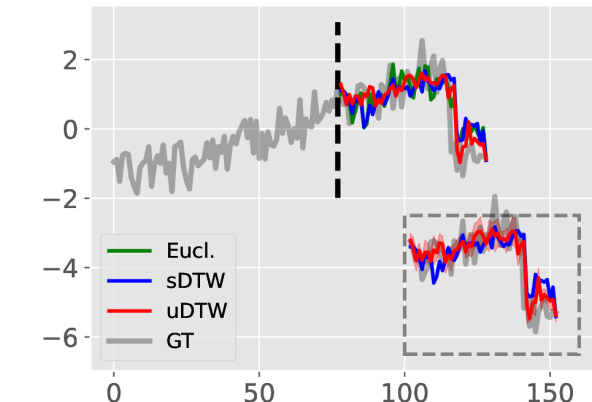
(a) CBF

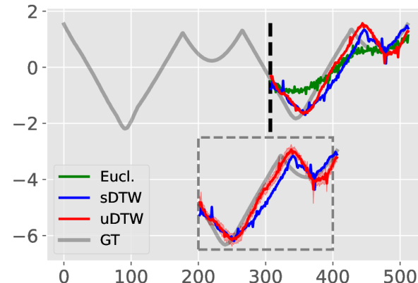
(b) ShapesAll

Figure 7: Additional visualizations for forecasting the evolution of time series. Given the first part of a time series, we train the pipeline from Fig. 3(b) to predict the remaining part of the time series. We compare the use of the Euclidean, sDTW or uDTW distances within the pipeline. We use CBF and ShapesAll in UCR archive, and display the prediction obtained for the given test sample with either of these 3 distances, and the ground truth (GT). Oftentimes, we observe that uDTW helps predict the sudden changes well. (a) Our uDTW aligns well with the ground truth compared to sDTW. (b) Our uDTW generates better shape of prediction compared to sDTW (for example note the red curve following much closer the rising gray slope). Quantitative results of MSE and ‘shape’ metrics for the whole UCR archive are given in the main paper.

We provide additional visualizations of forecasting the evolution of time series in Figure 7. We notice that our uDTW produces predictions that are better aligned with the ground truth (see Fig. 7(a)). Moreover, our uDTW generates better shape of the predictions compared to sDTW, and the predictions from sDTW have more perturbations/fluctuations (see Fig. 7(b)). Quantitative results for the whole UCR archive can be found in the main paper.

Appendix 0.F Additional Evaluations for Few-shot Action Recognition

Table 11: uDTW derived under the Normal, Laplacian and Cauchy distributions. Evaluations of few-shot action recognition on small-scale datasets.

	Supervised			Unsupervised
	MSR	3D Action Pairs	UWA 3D	MSR	3D Action Pairs	UWA 3D
TAP (HM) su2022temporal_sup	67.40	77.22	37.13	-	-	-
TAP (Lifted) su2022temporal_sup	65.20	78.33	34.80	-	-	-
TAP (Bino.) su2022temporal_sup	66.67	78.33	36.55	-	-	-
sDTW marco2017icml_sup	70.59	81.67	44.74	62.63	48.33	39.47
uDTW (Laplace)	72.24	82.89	45.64	66.00	55.00	41.22
uDTW (Cauchy)	70.88	84.44	45.03	65.12	50.32	40.50
uDTW (Normal)	72.66	83.33	47.66	65.00	52.22	41.74

Table 12: uDTW derived under the Normal, Laplacian and Cauchy distributions. Evaluations of few-shot action recognition on the large-scale NTU-60 dataset.

#classes	10	20	30	40	50
	Supervised
sDTW(baseline) marco2017icml_sup	53.7	56.2	60.0	63.9	67.8
uDTW(Cauchy)	56.1	61.1	62.9	68.3	69.9
uDTW(Laplace)	55.3	59.2	63.3	67.7	70.3
uDTW(Normal)	56.9	61.2	64.8	68.3	72.4
	Unsupervised
sDTW(baseline) marco2017icml_sup	35.6	45.2	53.3	56.7	61.7
uDTW(Cauchy)	36.7	47.9	54.9	57.3	63.3
uDTW(Laplace)	36.2	48.2	54.3	57.8	63.1
uDTW(Normal)	37.0	48.3	55.3	58.0	63.3

We also evaluate our proposed uDTW versus sDTW on smaller datasets for both supervised and unsupervised settings. As uDTW was derived in Section 1.2 under modeling the MLE of the product of the Normal distributions, we investigate modeling each path ${\bm{\Pi}}_{i}$ by replacing the Normal distribution with the Laplace or Cauchy distributions. By applying MLE principles in analogy to Section 1.2, we arrive at $\beta\Omega_{{\bm{\Pi}}_{i}}+d^{2}_{{\bm{\Pi}}_{i}}$ for

1. Laplace: $\sum_{(m,n)\in{\bm{\Pi}}_{i}}\beta\log(\sigma_{mn})+\frac{\|\bm{\psi}_{m}\!-\!\bm{\psi}^{\prime}_{n}\|_{1}}{\sigma_{mn}}$;

2. Cauchy: $\sum_{(m,n)\in{\bm{\Pi}}_{i}}\beta\log(\sigma_{mn})+\log\left(1+\frac{\|\bm{\psi}_{m}\!-\!\bm{\psi}^{\prime}_{n}\|_{2}^{2}}{\sigma^{2}_{mn}}\right)$.

Table 11 shows that uDTW achieves better performance than sDTW, and the Laplace distribution is performing particularly well on the unsupervised few-shot action recognition. Table 12 shows that uDTW based on the Normal distribution is overall better than other distributions on large-scale datasets such as NTU-60. For this very reason we use uDTW based on the Normal distribution.

Appendix 0.G Additional Visualizations on Barycenters

Figure 8 shows more visualizations of barycenters of time series. With our SigmaNet, we obtain much better barycenters with our uDTW compared to sDTW.

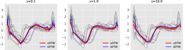
(a) ECG200

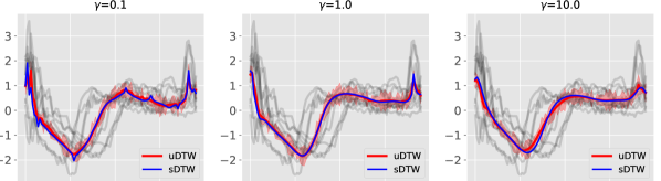
(b) ECG200 (our SigmaNet)

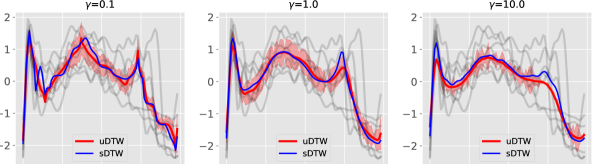
(c) Medical Images

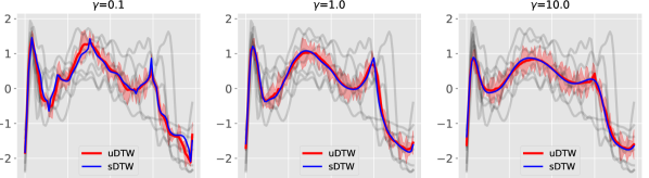
(d) Medical Images (our SigmaNet)

Figure 8: Comparison of barycenters based on our uDTW vs. sDTW. We visualize uncertainty around the barycenters in red color for uDTW. Our uDTW with SigmaNet generates reasonable barycenters even when higher $\gamma$ values are used, e.g., $\gamma\!=\!10.0$. Higher $\gamma$ value leads to smooth barycenters but introducing higher uncertainty.

Appendix 0.H Network Configuration and Training Details

Below we provide the details of network configuration and training process.

0.H.1 Skeleton Data Preprocessing

Before passing the skeleton sequences into MLP and a simple linear graph network (e.g., S²GC), we first normalize each body joint w.r.t. to the torso joint ${\bf v}_{f,c}$:

$${\bf v}^{\prime}_{f,i}\!=\!{\bf v}_{f,i}\!-\!{\bf v}_{f,c},$$ (23)

where $f$ and $i$ are the index of video frame and human body joint respectively. After that, we further normalize each joint coordinate into [-1, 1] range:

$$\hat{{\bf v}}_{f,i}[j]=\frac{{\bf v}^{\prime}_{f,i}[j]}{\text{max}([\text{abs}({\bf v}^{\prime}_{f,i}[j])]_{f\in{\mathcal{I}_{\tau}},i\in\mathcal{I}_{J}})},$$ (24)

where $j$ is for selection of the $x$, $y$ and $z$ axes, $\tau$ is the number of frames and $J$ is the number of 3D body joints per frame.

For the skeleton sequences that have more than one performing subject, (i) we normalize each skeleton separately, and each skeleton is passed to MLP for learning the temporal dynamics, and (ii) for the output features per skeleton from MLP, we pass them separately to the graph neural network, e.g., two skeletons from a given video sequence will have two outputs obtained from the graph neural network, and we aggregate the outputs through average pooling before passing to sDTW or uDTW.

0.H.2 Network Configuration

SigmaNet. It is composed of an FC layer and a scaled sigmoid function which translate the learned features of either actions or time series into desired $\bm{\Sigma}$. The input to FC is of the size of feature dimension (depends on the encoder) and the output is a scalar. SigmaNet with the scaled sigmoid function can be defined as:

$$\sigma(\bm{\psi})\!=\!\frac{\kappa}{1\!+\!\exp({-\text{FC}(\bm{\psi})})}\!+\!\eta,$$ (25)

where $\eta\!>\!0$ is the offset and $\kappa\!\geq\!0$ is the maximum magnitude of sigmoid. For an entire sequence with $\tau$ blocks, the SigmaNet produces vector $\bm{\sigma}_{\mathbf{x}}$ for sequence $\mathbf{x}$ and $\bm{\sigma}_{\mathbf{x}^{\prime}}$ for sequence $\mathbf{x}^{\prime}$ (we concatenate per-block scalars to form these vectors), and we typically obtain $\bm{\Sigma}\!=\!\bm{\sigma}^{2}_{\mathbf{x}}\textbf{1}^{\top}\!+\!{\mathbf{1}\bm{\sigma}^{2}_{\mathbf{x}^{\prime}}}^{\!\top}$.

Forecasting of the evolution of time series.

The MLP for this task consists of two FC layers with a tanh layer in between. The input to the first FC layer is $t$ and output size is $t^{\prime}$, and after the tanh layer, the input to the second FC layer is $t^{\prime}$ and output $(\tau\!-\!t)$ dimensional prediction. We set $t^{\prime}\!=30$ or 50 depending on the length of time series in each dataset.

Few-shot action recognition.

Given the temporal block size $M$ (the number of frames in a block) and desired output size $d$, the configuration of the 3-layer MLP unit is: FC ($3M\rightarrow 6M$), LayerNorm (LN) as in [11], ReLU, FC ($6M\rightarrow 9M$), LN, ReLU, Dropout (for smaller datasets, the dropout rate is 0.5; for large-scale datasets, the dropout rate is 0.1), FC ($9M\rightarrow d$), LN. Note that $M$ is the temporal block size  and $d$ is the output feature dimension per body joint. We set $M\!=\!10$ for experiments.

For the encoding network, let us take the query input $\mathbf{X}\!\in\!\mathbb{R}^{3\times J\times M}$ for the temporal block of length $M$ as an example, where $3$ indicates that Cartesian coordinates $(x,y,z)$ were used, and $J$ is the number of body joints. As alluded to earlier, we obtain $\widehat{\mathbf{X}}^{T}\!=\!\text{MLP}(\mathbf{X};\mathcal{P}_{MLP})\!\in\!\mathbb{R}^{{d}\times J}$.

Subsequently, we employ a simple linear graph network, S²GC from Section 0.H.3, and the transformer encoder [11] which consists of alternating layers of Multi-Head Self-Attention (MHSA) and a feed-forward MLP (two FC layers with a GELU non-linearity between them). LayerNorm (LN) is applied before every block, and residual connections after every block. Each block feature matrix $\widehat{\mathbf{X}}\in\mathbb{R}^{J\times{d}}$ encoded by a simple linear graph network S²GC (without learnable $\bf\Theta$) is then passed to the transformer. Similarly to the standard transformer, we prepend a learnable vector ${\bf y}_{\text{token}}\!\in\!\mathbb{R}^{1\times{d}}$ to the sequence of block features $\widehat{\mathbf{X}}$ obtained from S²GC, and we also add the positional embeddings ${\bf E}_{\text{pos}}\in\mathbb{R}^{(1+J)\times{d}}$ based on the sine and cosine functions (standard in transformers) so that token ${\bf y}_{\text{token}}$ and each body joint enjoy their own unique positional encoding. We obtain $\mathbf{Z}_{0}\!\in\!\mathbb{R}^{(1+J)\times{d}}$ which is the input in the following backbone:

$${\bf Z}_{0}=[{\bf y}_{\text{token}};\text{S\textsuperscript{2}GC}(\widehat{\mathbf{X}})]+{\bf E}_{\text{pos}},$$ (26)

$${\bf Z}^{\prime}_{k}=\text{MHSA}(\text{LN}({\bf Z}_{k-1}))+{\bf Z}_{k-1},\;k=1,...,L_{\text{tr}}$$ (27)

$${\bf Z}_{k}=\text{MLP}(\text{LN}({\bf Z}^{\prime}_{k}))+{\bf Z}^{\prime}_{k},\qquad\quad\,k=1,...,L_{\text{tr}}$$ (28)

$$\mathbf{y}^{\prime}=\text{LN}\big{(}\mathbf{Z}^{(0)}_{L_{\text{tr}}}\big{)}\qquad\qquad\text{ where }\quad\;\;\mathbf{y}^{\prime}\in\mathbb{R}^{1\times{d}}$$ (29)

$$f(\mathbf{X};\mathcal{P})=\text{FC}(\mathbf{y}^{\prime T};\mathcal{P}_{FC})\qquad\qquad\quad\!\in\mathbb{R}^{d^{\prime}},$$ (30)

where $\mathbf{Z}^{(0)}_{L_{\text{tr}}}$ is the first ${d}$ dimensional row vector extracted from the output matrix $\mathbf{Z}_{L_{\text{tr}}}$ of size $(J\!+\!1)\times{d}$ which corresponds to the last layer $L_{\text{tr}}$ of the transformer. Moreover, parameter $L_{\text{tr}}$ controls the depth of the transformer, whereas $\mathcal{P}\!\equiv\![\mathcal{P}_{MLP},\mathcal{P}_{S\textsuperscript{2}GC},\mathcal{P}_{Transf},\mathcal{P}_{FC}]$ is the set of parameters of EN. In case of S²GC, $|\mathcal{P}_{S\textsuperscript{2}GC}|\!=\!0$ because we do not use their learnable parameters $\bf\Theta$ (i.e., think $\bf\Theta$ is set as the identity matrix in Eq. (31)).

We can define now a support feature map as $\bm{\Psi}^{\prime}\!=\![f(\bm{X}_{1};\mathcal{P}),...,f(\bm{X}_{\tau^{\prime}};\mathcal{P})]\!\in\!\mathbb{R}^{d^{\prime}\times\tau^{\prime}}$ for $\tau^{\prime}$ temporal blocks, and the query map $\bm{\Psi}$ accordingly.

The hidden size of our transformer (the output size of the first FC layer of the MLP depends on the dataset. For smaller datasets, the depth of the transformer is $L_{\text{tr}}\!=\!6$ with $64$ as the hidden size, and the MLP output size is ${d}\!=\!32$ (note that the MLP which provides $\widehat{\mathbf{X}}$ and the MLP in the transformer must both have the same output size). For NTU-60, the depth of the transformer is $L_{\text{tr}}\!=\!6$, the hidden size is 128 and the MLP output size is ${d}\!=\!64$. For NTU-120, the depth of the transformer is $L_{\text{tr}}\!=\!6$, the hidden size is 256 and the MLP size is ${d}\!=\!128$. For Kinetics-skeleton, the depth for the transformer is $L_{\text{tr}}\!=\!12$, hidden size is 512 and the MLP output size is ${d}\!=\!256$. The number of Heads for the transformer of smaller datasets, NTU-60, NTU-120 and Kinetics-skeleton is set as 6, 12, 12 and 12, respectively.

The output sizes $d^{\prime}$ of the final FC layer are 50, 100, 200, and 500 for the smaller datasets, NTU-60, NTU-120 and Kinetics-skeleton, respectively.

0.H.3 Linear Graph Network (S²GC)

Based on a modified Markov Diffusion Kernel, Simple Spectral Graph Convolution (S²GC) is the summation over $l$-hops, $l\!=\!1,...,L$. The output of S²GC is given as:

$${\bf\Phi_{\text{S\textsuperscript{2}GC}}}\!=\!\frac{1}{L}\sum_{l=1}^{L}((1\!-\!\alpha){\bf S}^{l}{\bf X}\!+\!\alpha{\bf X}){\bf\Theta},$$ (31)

where $L\!\geq\!1$ is the number of linear layers and $\alpha\!\geq\!0$ determines the importance of self-loop of each node (we use their default setting $\alpha\!=\!0.05$ and $L\!=\!6$). Choice of other graph embeddings are possible, including contrastive models COLES zhu2021contrastive_sup or COSTA costa_sup, adversarial Fisher-Bures GCN uai_ke_sup or GCNs with rectifier attention www_sup. One may also use kernels on 3D body joints as in action_domain_sup or even use CNN to encode 3D body joints as COLTRANE coltrane_sup.

0.H.4 $K$-NN classifier with SoftMax

For the $K$-NN classifier, instead of using $K$ best weights proportional to the inverse of the distance from the query sample $\mathbf{x}^{*}$ to the closest samples $\mathbf{x}_{n}$ (as is done in the soft-DTW paper marco2017icml_sup) and expressed by

$$w(\mathbf{x}_{n}|\mathbf{x}^{*})=\frac{1}{d^{2}\big{(}\mathbf{x}^{*},\mathbf{x}_{n}\big{)}},$$ (32)

we weigh the neighbors $\mathbf{x}_{n}$ of $\mathbf{x}^{*}$ using

$$w(\mathbf{x}_{n}|\mathbf{x}^{*})=\frac{\text{exp}\big{(}-\frac{1}{\gamma^{\prime\prime}}d^{2}\big{(}\mathbf{x}^{*},\mathbf{x}_{n}\big{)}\big{)}}{\sum_{n^{\prime}\in\mathcal{N}(\mathbf{x}^{*};K)}\text{exp}\big{(}-\frac{1}{\gamma^{\prime\prime}}d^{2}\big{(}\mathbf{x}^{*},\mathbf{x}_{n^{\prime}}\big{)}\big{)}}$$ (33)

such that $\mathcal{N}(\mathbf{x}^{*};K)$ produces $K$ nearest samples $\mathbf{x}_{n^{\prime}}$ of $\mathbf{x}^{*}$ according to distance $d(\cdot,\cdot)$, e.g., the Euclidean distance, sDTW or uDTW. Parameter $\gamma^{\prime\prime}\!>\!0$ (in our case, we set $\gamma^{\prime\prime}\!=\!6$) further controls the impact of each sample $\mathbf{x}_{n}$ on the classifier based on the bell shape of Radial Basis Function in the above equation.

Table 13 shows the comparisons. We notice that the use of SoftMax in the $K$-NN classifier improves the performance for all the methods when $K\!=\!3$ and $K\!=\!5$.

Table 13: Classification accuracy (mean$\pm$std) on UCR archive using nearest neighbor. $K$ denotes the number of nearest neighbors in the $K$-NN classifier. Highlighted rows are the based on SoftMax from Eq. (33). Non-highlighted rows are based on Eq. (32).

	Nearest neighbor
	$K=1$	$K=3$	$K=5$
Euclidean	71.2$\pm$17.5	69.5$\pm$18.0	67.5$\pm$17.6
Euclidean (SoftMax)	71.2$\pm$17.5	72.3$\pm$18.1	73.0$\pm$16.7
DTW marco2011icml_sup	74.2$\pm$16.6	72.8$\pm$16.9	71.4$\pm$16.8
DTW marco2011icml_sup (SoftMax)	74.2$\pm$16.6	75.0$\pm$17.0	75.4$\pm$15.8
sDTW marco2017icml_sup	76.2$\pm$16.6	74.0$\pm$15.6	70.5$\pm$17.6
sDTW marco2017icml_sup (SoftMax)	76.2$\pm$16.6	77.2$\pm$15.9	78.0$\pm$16.5
sDTW div. pmlr-v130-blondel21a_sup	78.6$\pm$16.2	76.5$\pm$16.4	74.8$\pm$15.8
sDTW div. pmlr-v130-blondel21a_sup (SoftMax)	78.6$\pm$16.2	79.5$\pm$16.7	80.1$\pm$16.5
uDTW	80.0$\pm$15.0	78.0$\pm$15.8	76.2$\pm$15.0
uDTW (SoftMax)	80.0$\pm$15.0	81.2$\pm$17.8	83.3$\pm$16.2

0.H.5 Training Details

For both time series and few-shot action recognition pipelines, the weights are initialized with the normal distribution (zero mean and unit standard deviation). We use 1e-3 for the learning rate, and the weight decay is 1e-6. We use the SGD optimizer.

For time series, we set the training epochs to 30, 50 and 100 depending on the dataset in the UCR archive (due to many datasets, the epoch settings will be provided in the code directly).

For few-shot action recognition, we set the number of training episodes to 100K for NTU-60, 200K for NTU-120, 500K for 3D Kinetics-skeleton, 10K for small datasets such as UWA 3D Multiview Activity II.

Appendix 0.I Hyperparameters Evaluation

In this section, we evaluate the impact of key hyperparameters. Remaining hyperparameters are obtained through Hyperopt bergstra2015hyperopt for hyperparameter search on the validation set.

0.I.1 Evaluation of $\bm{\Sigma}$

We compare results given different formulations of $\bm{\Sigma}$ in Tables 14 and 15. We notice that on smaller datasets, it is hard to determine which variant of $\bm{\Sigma}$ is better (as these earlier datasets have fewer limited reliable skeletons compared to the new datasets). However, on bigger datasets, $\bm{\Sigma}\!=\!\bm{\sigma}^{2}_{\bm{\psi}}\bm{1}^{\top}\!\!+\!\bm{1}{\bm{\sigma}_{\bm{\psi}^{\prime}}^{\top}}^{\!2}$ performs the best in all cases; thus we choose this formulation of $\bm{\Sigma}$ for large-scale datasets.

Table 14: Evaluation of different variants of $\bm{\Sigma}$ computation on small-scale datasets (supervised few-shot action recognition). Operator $\odot$ is the Hadamart product.

	$\;\bm{\sigma}_{\bm{\psi}}\bm{1}^{\top}\!\!\!\odot\!\bm{1}{\bm{\sigma}_{\bm{\psi}^{\prime}}^{\top}}\;$	$\;\bm{\sigma}^{2}_{\bm{\psi}}\bm{1}^{\top}\!\!\!\odot\!\bm{1}{\bm{\sigma}_{\bm{\psi}^{\prime}}^{\top}}^{\!2}\;$	$\;\bm{\sigma}_{\bm{\psi}}\bm{1}^{\top}\!\!\!+\!\bm{1}{\bm{\sigma}_{\bm{\psi}^{\prime}}^{\top}}\;$	$\;\bm{\sigma}^{2}_{\bm{\psi}}\bm{1}^{\top}\!\!\!+\!\bm{1}{\bm{\sigma}_{\bm{\psi}^{\prime}}^{\top}}^{\!2}$
MSR Action 3D	72.32	68.51	70.59	69.20
3D Action Pairs	82.78	80.56	82.22	85.00
UWA 3D Activity	43.86	45.91	45.91	45.03

Table 15: Evaluation of different variants of $\bm{\Sigma}$ computation on the large-scale NTU-60 dataset (supervised few-shot action recognition).

#classes	$\;\bm{\sigma}_{\bm{\psi}}\bm{1}^{\top}\!\!\!\odot\!\bm{1}{\bm{\sigma}_{\bm{\psi}^{\prime}}^{\top}}\;$	$\;\bm{\sigma}^{2}_{\bm{\psi}}\bm{1}^{\top}\!\!\!\odot\!\bm{1}{\bm{\sigma}_{\bm{\psi}^{\prime}}^{\top}}^{\!2}\;$	$\;\bm{\sigma}_{\bm{\psi}}\bm{1}^{\top}\!\!\!+\!\bm{1}{\bm{\sigma}_{\bm{\psi}^{\prime}}^{\top}}\;$	$\;\bm{\sigma}^{2}_{\bm{\psi}}\bm{1}^{\top}\!\!\!+\!\bm{1}{\bm{\sigma}_{\bm{\psi}^{\prime}}^{\top}}^{\!2}$
$10$	56.6	56.0	55.6	56.9
$20$	60.4	61.0	61.2	61.2
$30$	64.2	64.1	63.5	64.8
$40$	68.1	66.9	67.2	68.3
$50$	72.0	72.3	72.0	72.4

0.I.2 Evaluation of $\kappa$ and $\eta$ of SigmaNet

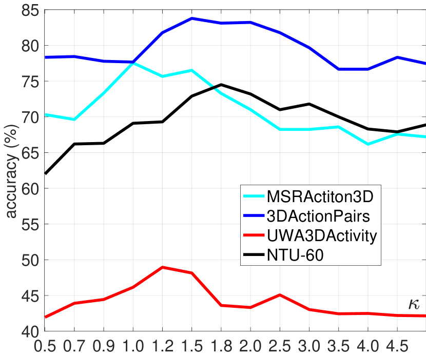
(a)

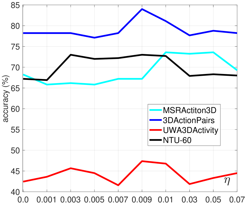
(b)

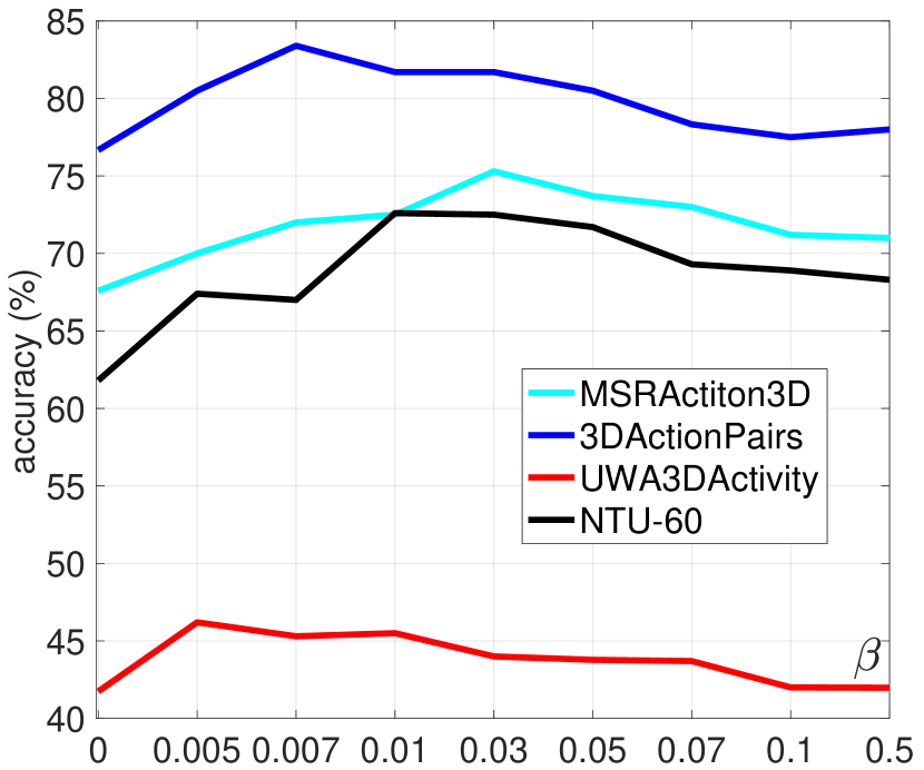
(c)

Figure 9: Evaluation of (a) $\kappa$ which controls the maximum magnitude and (b) $\eta$ offset from Eq. (25) in SigmaNet and (c) $\beta$ from Eq. (22). Note that $\beta\!=\!0$ means no regularization term of uDTW in use. We notice that with the regularization term added to the uDTW, the overall performance is improved.

Figures 9(a) and 9(b) show the impact of $\kappa$ and $\eta$ of the scaled sigmoid function in SigmaNet on both small-scale datasets and the large-scle NTU-60 dataset. We notice that $\kappa\!=\!1.5$ performs the best on the three small-scale datasets and $\kappa\!=\!1.8$ works the best on NTU-60. We choose $\kappa\!=\!1.8$ in the experiments for the large-scale datasets. Moreover, $\eta\!\in\![0.003,0.01]$ works better on NTU-60, and on the small-scale datasets, $\eta\!=\!0.01$ achieves the best performance; thus we choose $\eta\!=\!0.01$ for the experiments.

0.I.3 Evaluation of $\beta$

Figure 9(c) shows the evaluations of $\beta$ for both small-scale datasets and NTU-60. Firstly, note that $\beta\!=\!0$ means lack of the regularization term of uDTW, which immediately causes the performance deterioration. As shown in the figure, $\beta\!=\!0.05$ performs the best on UWA 3D Activity, $\beta\!=\!0.03$ achieves the best performance on MSR Action 3D and $\beta\!=\!0.007$ works the best on 3D Action Pairs dataset. We use the corresponding best $\beta$ values for the smaller datasets. On NTU-60, $\beta\!\in\![0.01,0.05]$ performs the best compared to other $\beta$ values, thus we choose $\beta\!=\!0.03$ for the experiments on all large-scale datasets.

0.I.4 Evaluation of warping window width

Table 16 on ECGFiveDays (from UCR) and NTU-60 (50-class, supervised / unsup. settings) shows that uDTW does not break quicker than sDTW (window size is parametrized by $r$). Very small $r$ may preclude backpropagating through some paths (of large distance). For such paths ‘beyond window’, learning uncertainty is limited but this is normal. For similar reasons, choosing the right window size is required by other DTW variants too. Also, if $r$ is very large, large uncertainty score may decrease the distance on multitude of paths by downweighting parts of paths (could lead to strange matching) but as the uncertainty is aggregated into the regularization penalty, this penalty prevents uDTW from unreasonable solutions. Lack of regularization penalty (w/o reg.) affects the most the unsupervised few-shot learning, while supervised loss can still drive SigmaNet to produce meaningful results.

Table 16: Experimental results on ECGFiveDays (from UCR) and NTU-60 (50-class, supervised / unsup. settings) for different warping window widths.

		$\gamma=0.001$			$\gamma=0.01$			$\gamma=0.1$			$\gamma=1$
		$r$=1.0	$r$=3.0	$r$=5.0	$r$=1.0	$r$=3.0	$r$=5.0	$r$=1.0	$r$=3.0	$r$=5.0	$r$=1.0	$r$=3.0	$r$=5.0
$\begin{subarray}{c}\text{ECG}\\ \text{FiveDays}\end{subarray}$	sDTW	83.4	82.8	82.0	79.7	76.8	77.8	75.4	69.0	65.3	62.5	61.7	60.2
	uDTW	85.6	91.2	81.0	93.5	82.8	80.6	79.7	73.9	67.3	69.0	65.3	62.5
	$\begin{subarray}{c}\text{uDTW}\\ \text{{\it w/o reg.}}\end{subarray}$	75.4	74.0	69.0	79.7	77.9	76.8	65.3	62.5	61.5	61.2	62.0	60.2
$\begin{subarray}{c}\text{NTU-60}\\ \text{(sup.)}\end{subarray}$	sDTW	65.7	64.7	64.8	65.2	67.8	63.9	60.0	58.9	54.3	54.0	52.2	52.3
	uDTW	71.5	71.0	70.0	72.4	72.4	70.0	68.3	66.7	67.8	65.7	64.8	66.8
	$\begin{subarray}{c}\text{uDTW}\\ \text{{\it w/o reg.}}\end{subarray}$	66.3	65.0	65.5	66.4	68.0	65.2	62.0	59.2	55.0	52.0	52.0	51.2
$\begin{subarray}{c}\text{NTU-60}\\ \text{(unsup.)}\end{subarray}$	sDTW	56.7	53.2	50.0	61.7	61.7	60.0	54.4	52.5	52.1	48.3	45.2	40.9
	uDTW	61.0	61.5	60.7	63.3	63.0	62.5	59.2	59.0	57.3	58.0	57.2	55.7
	$\begin{subarray}{c}\text{uDTW}\\ \text{{\it w/o reg.}}\end{subarray}$	50.1	49.3	47.0	55.3	54.0	51.3	44.1	42.0	40.7	42.3	40.1	35.6

splncs04 egbib

See pages - of 5350_present.pdf

References

- [1] Abid, A., Zou, J.: Autowarp: Learning a warping distance from unlabeled time series using sequence autoencoders. NIPS’18, Curran Associates Inc., Red Hook, NY, USA (2018)
- [2] Ben-Ari, R., Shpigel Nacson, M., Azulai, O., Barzelay, U., Rotman, D.: Taen: Temporal aware embedding network for few-shot action recognition. In: 2021 IEEE/CVF Conference on Computer Vision and Pattern Recognition Workshops (CVPRW). pp. 2780–2788 (2021)
- [3] Blondel, M., Mensch, A., Vert, J.P.: Differentiable divergences between time series. In: Banerjee, A., Fukumizu, K. (eds.) Proceedings of The 24th International Conference on Artificial Intelligence and Statistics. Proceedings of Machine Learning Research, vol. 130, pp. 3853–3861. PMLR (13–15 Apr 2021)
- [4] Cao, K., Ji, J., Cao, Z., Chang, C.Y., Niebles, J.C.: Few-shot video classification via temporal alignment. In: CVPR (2020)
- [5] Catalin, Ionescu, Dragos, Papava, Vlad, Olaru, Cristian, Sminchisescu: Human3.6m: Large scale datasets and predictive methods for 3d human sensing in natural environments. IEEE Transactions on Pattern Analysis & Machine Intelligence (2014)
- [6] Cuturi, M.: Fast global alignment kernels. In: International Conference on Machine Learning (ICML) (2011)
- [7] Cuturi, M., Blondel, M.: Soft-dtw: a differentiable loss function for time-series. In: International Con- ference on Machine Learning (ICML) (2017)
- [8] Dau, H.A., Keogh, E., Kamgar, K., Yeh, C.C.M., Zhu, Y., Gharghabi, S., Ratanamahatana, C.A., Yanping, Hu, B., Begum, N., Bagnall, A., Mueen, A., Batista, G.: The UCR Time Series Classification Archive (October 2018), https://www.cs.ucr.edu/~eamonn/time_series_data_2018/
- [9] Dempster, A., Schmidt, D.F., Webb, G.I.: Minirocket: A very fast (almost) deterministic transform for time series classification. In: Proceedings of the 27th ACM SIGKDD Conference on Knowledge Discovery & Data Mining. p. 248–257. KDD ’21, Association for Computing Machinery, New York, NY, USA (2021). https://doi.org/10.1145/3447548.3467231
- [10] Donahue, J., Dieleman, S., Binkowski, M., Elsen, E., Simonyan, K.: End-to-end adversarial text-to-speech. In: International Conference on Learning Representations (2021)
- [11] Dosovitskiy, A., Beyer, L., Kolesnikov, A., Weissenborn, D., Zhai, X., Unterthiner, T., Dehghani, M., Minderer, M., Heigold, G., Gelly, S., et al.: An image is worth 16x16 words: Transformers for image recognition at scale. In: International Conference on Learning Representations (2020)
- [12] García-García, D., Parrado Hernández, E., Díaz-de María, F.: A new distance measure for model-based sequence clustering. IEEE Transactions on Pattern Analysis and Machine Intelligence 31(7), 1325–1331 (2009). https://doi.org/10.1109/TPAMI.2008.268
- [13] Hastie, T., Tibshirani, R., Friedman, J.: The Elements of Statistical Learning. Springer Series in Statistics, Springer New York Inc., New York, NY, USA (2001)
- [14] Hüllermeier, E., Waegeman, W.: Aleatoric and epistemic uncertainty in machine learning: an introduction to concepts and methods. Mach. Learn. 110(3), 457–506 (2021). https://doi.org/10.1007/s10994-021-05946-3
- [15] Indrayan, A.: Medical biostatistics. Chapman & Hall/CRC,, Boca Raton :, 2nd ed. edn. (c2008), http://www.loc.gov/catdir/toc/ecip0723/2007030353.html
- [16] Kay, W., Carreira, J., Simonyan, K., Zhang, B., Hillier, C., Vijayanarasimhan, S., Viola, F., Green, T., Back, T., Natsev, P., Suleyman, M., Zisserman, A.: The kinetics human action video dataset (2017)
- [17] Kendall, A., Gal, Y.: What uncertainties do we need in bayesian deep learning for computer vision? In: Guyon, I., Luxburg, U.V., Bengio, S., Wallach, H., Fergus, R., Vishwanathan, S., Garnett, R. (eds.) Advances in Neural Information Processing Systems. vol. 30. Curran Associates, Inc. (2017)
- [18] Kiureghian, A.D., Ditlevsen, O.: Aleatory or epistemic? does it matter? Structural Safety 31(2), 105–112 (2009). https://doi.org/https://doi.org/10.1016/j.strusafe.2008.06.020, risk Acceptance and Risk Communication
- [19] Koniusz, P., Mikolajczyk, K.: Soft assignment of visual words as linear coordinate coding and optimisation of its reconstruction error. In: 2011 18th IEEE International Conference on Image Processing. pp. 2413–2416 (2011). https://doi.org/10.1109/ICIP.2011.6116129
- [20] Koniusz, P., Wang, L., Cherian, A.: Tensor representations for action recognition. TPAMI (2020)
- [21] Koniusz, P., Yan, F., Mikolajczyk, K.: Comparison of mid-level feature coding approaches and pooling strategies in visual concept detection. Computer Vision and Image Understanding 117(5), 479–492 (2013). https://doi.org/https://doi.org/10.1016/j.cviu.2012.10.010
- [22] Li, S., Liu, H., Qian, R., Li, Y., See, J., Fei, M., Yu, X., Lin, W.: TTAN: two-stage temporal alignment network for few-shot action recognition. CoRR (2021)
- [23] Liu, D.C., Nocedal, J.: On the limited memory bfgs method for large scale optimization. Mathematical Programming 45, 503–528 (1989)
- [24] Liu, J., Shahroudy, A., Perez, M., Wang, G., Duan, L.Y., Kot, A.C.: Ntu rgb+d 120: A large-scale benchmark for 3d human activity understanding. IEEE Transactions on Pattern Analysis and Machine Intelligence (2019). https://doi.org/10.1109/TPAMI.2019.2916873
- [25] Liu, L., Wang, L., Liu, X.: In defense of soft-assignment coding. In: 2011 International Conference on Computer Vision. pp. 2486–2493 (2011). https://doi.org/10.1109/ICCV.2011.6126534
- [26] Lohit, S., Wang, Q., Turaga, P.: Temporal transformer networks: Joint learning of invariant and discriminative time warping. In: Proceedings of the IEEE/CVF Conference on Computer Vision and Pattern Recognition (CVPR) (June 2019)
- [27] Martinez, J., Hossain, R., Romero, J., Little, J.J.: A simple yet effective baseline for 3d human pose estimation. In: 2017 IEEE International Conference on Computer Vision (ICCV). pp. 2659–2668 (2017). https://doi.org/10.1109/ICCV.2017.288
- [28] Matthies, H.G.: Quantifying uncertainty: Modern computational representation of probability and applications. In: Ibrahimbegovic, A., Kozar, I. (eds.) Extreme Man-Made and Natural Hazards in Dynamics of Structures. pp. 105–135. Springer Netherlands, Dordrecht (2007)
- [29] Memmesheimer, R., Häring, S., Theisen, N., Paulus, D.: Skeleton-dml: Deep metric learning for skeleton-based one-shot action recognition (2021)
- [30] Memmesheimer, R., Theisen, N., Paulus, D.: Signal level deep metric learning for multimodal one-shot action recognition (2020)
- [31] Mensch, A., Blondel, M.: Differentiable dynamic programming for structured prediction and attention. In: Dy, J., Krause, A. (eds.) Proceedings of the 35th International Conference on Machine Learning. Proceedings of Machine Learning Research, vol. 80, pp. 3462–3471. PMLR (10–15 Jul 2018)
- [32] Mina, B., Zoumpourlis, G., Patras, I.: Tarn: Temporal attentive relation network for few-shot and zero-shot action recognition. In: Sidorov, K., Hicks, Y. (eds.) Proceedings of the British Machine Vision Conference (BMVC). pp. 130.1–130.14. BMVA Press (September 2019). https://doi.org/10.5244/C.33.130
- [33] Perrett, T., Masullo, A., Burghardt, T., Mirmehdi, M., Damen, D.: Temporal-relational crosstransformers for few-shot action recognition. In: Proceedings of the IEEE/CVF Conference on Computer Vision and Pattern Recognition (CVPR). pp. 475–484 (June 2021)
- [34] Ramachandran, P., Liu, P.J., Le, Q.V.: Unsupervised pretraining for sequence to sequence learning (2018)
- [35] Sakoe, H., Chiba, S.: Dynamic programming algorithm optimization for spoken word recognition. IEEE Transactions on Acoustics, Speech, and Signal Processing 26(1), 43–49 (1978). https://doi.org/10.1109/TASSP.1978.1163055
- [36] Shahroudy, A., Liu, J., Ng, T.T., Wang, G.: Ntu rgb+d: A large scale dataset for 3d human activity analysis. In: IEEE Conference on Computer Vision and Pattern Recognition (June 2016)
- [37] Snell, J., Swersky, K., Zemel, R.S.: Prototypical networks for few-shot learning. In: Guyon, I., von Luxburg, U., Bengio, S., Wallach, H.M., Fergus, R., Vishwanathan, S.V.N., Garnett, R. (eds.) Advances in Neural Information Processing Systems 30: Annual Conference on Neural Information Processing Systems 2017, 4-9 December 2017, Long Beach, CA, USA. pp. 4077–4087 (2017)
- [38] Su, B., Hua, G.: Order-preserving optimal transport for distances between sequences. IEEE Transactions on Pattern Analysis and Machine Intelligence 41(12), 2961–2974 (2019). https://doi.org/10.1109/TPAMI.2018.2870154
- [39] Su, B., Wen, J.R.: Temporal alignment prediction for supervised representation learning and few-shot sequence classification. In: International Conference on Learning Representations (2022)
- [40] Su, B., Zhou, J., Wu, Y.: Order-preserving wasserstein discriminant analysis. In: 2019 IEEE/CVF International Conference on Computer Vision (ICCV). pp. 9884–9893 (2019). https://doi.org/10.1109/ICCV.2019.00998
- [41] Tan, S., Yang, R.: Learning similarity: Feature-aligning network for few-shot action recognition. In: International Joint Conference on Neural Networks (IJCNN). pp. 1–7 (2019)
- [42] Vinyals, O., Blundell, C., Lillicrap, T., Kavukcuoglu, K., Wierstra, D.: Matching networks for one shot learning. In: Lee, D.D., Sugiyama, M., von Luxburg, U., Guyon, I., Garnett, R. (eds.) Advances in Neural Information Processing Systems 29: Annual Conference on Neural Information Processing Systems 2016, December 5-10, 2016, Barcelona, Spain. pp. 3630–3638 (2016)
- [43] Wang, L.: Analysis and Evaluation of Kinect-based Action Recognition Algorithms. Master’s thesis, School of the Computer Science and Software Engineering, The University of Western Australia (Nov 2017)
- [44] Wang, L., Huynh, D.Q., Koniusz, P.: A comparative review of recent kinect-based action recognition algorithms. IEEE Transactions on Image Processing 29, 15–28 (2020)
- [45] Wang, L., Huynh, D.Q., Mansour, M.R.: Loss switching fusion with similarity search for video classification. ICIP (2019)
- [46] Wang, L., Koniusz, P.: Self-Supervising Action Recognition by Statistical Moment and Subspace Descriptors, p. 4324–4333. Association for Computing Machinery, New York, NY, USA (2021), https://doi.org/10.1145/3474085.3475572
- [47] Wang, L., Koniusz, P., Huynh, D.Q.: Hallucinating IDT descriptors and I3D optical flow features for action recognition with cnns. In: The IEEE International Conference on Computer Vision (ICCV) (October 2019)
- [48] Yan, S., Xiong, Y., Lin, D.: Spatial Temporal Graph Convolutional Networks for Skeleton-Based Action Recognition. In: AAAI (2018)
- [49] Yang, C.H.H., Tsai, Y.Y., Chen, P.Y.: Voice2series: Reprogramming acoustic models for time series classification. In: Meila, M., Zhang, T. (eds.) Proceedings of the 38th International Conference on Machine Learning. Proceedings of Machine Learning Research, vol. 139, pp. 11808–11819. PMLR (18–24 Jul 2021)
- [50] Zhang, H., Zhang, L., Qi, X., Li, H., Torr, P., Koniusz, P.: Few-shot action recognition with permutation-invariant attention. In: European Conference on Computer Vision (ECCV) (2020)
- [51] Zhu, H., Koniusz, P.: Simple spectral graph convolution. In: International Conference on Learning Representations (ICLR) (2021)