Progress in the numerical studies of the type IIB matrix model
Abstract
The type IIB matrix model, also known as the IKKT model, has been proposed as a promising candidate for a non-perturbative formulation of superstring theory. Based on this proposal, various attempts have been made to explain how our four-dimensional space-time can emerge dynamically from superstring theory. In this article, we review the progress in numerical studies on the type IIB matrix model. We particularly focus on the most recent results for the Euclidean and Lorentzian versions, which are obtained using the complex Langevin method to overcome the sign problem. We also review the earlier results obtained using conventional Monte Carlo methods and clarify the relationship among different calculations.
1 Introduction
The type IIB matrix model, also known as the IKKT model 9612115 , is regarded as one of the most promising candidates for a non-perturbative formulation of superstring theory. The model is defined by dimensionally reducing ten-dimensional super Yang–Mills theory to zero dimensions. Therefore, space-time does not exist a priori in this model. We interpret the eigenvalues of the bosonic matrices as the space-time coordinates, and hence, space-time is generated dynamically from the degrees of freedom of the matrices Aoki:1998vn . Since superstring theory is defined in ten dimensions, it is important to understand how our four-dimensional space-time emerges by studying this model.
Various attempts have been made to address this question. In the Lorentzian version of the type IIB matrix model, the indices are contracted by the metric , and the action has the SO(9,1) symmetry. The bosonic action is unbounded from below, and this is why no one has dared to study the Lorentzian version numerically for a long time. Instead, the efforts have been focused on the Euclidean version 9811220 ; 0003208 ; 0005147 ; 0108041 ; 1009_4504 ; 1108_1534 ; 1306_6135 ; 1509_05079 ; 1712_07562 ; 2002_07410 , which is defined by making a Wick rotation with respect to the temporal direction, and contracting the indices by the Euclidean metric .
The Euclidean version has the SO(10) rotational symmetry instead of the SO(9,1), and it is amenable to numerical simulations because the partition function is finite without any cutoffs 9803117 ; 0103159 . However, it suffers from a severe sign problem, which appears after integrating out the fermions. The complex Pfaffian (determinant in the simplified four or six-dimensional SUSY models) plays a central role in the spontaneous symmetry breaking (SSB) of the SO(10) rotational symmetry 0003223 ; Nishimura:2000wf . In models where there are no fermionic degrees of freedom, like the bosonic model, or the Pfaffian is real positive, like in the four-dimensional SUSY model, there is no SSB of the rotational symmetry 9811220 ; 0003208 ; Ambjorn:2001xs . There is no SSB, either, in the phase-quenched model, which omits the complex phase of the Pfaffian 1509_05079 . Thus, to study the SSB of the rotational symmetry, one should take into account the complex phase, for instance by reweighting, in which case the important configurations are generally different between the original model and its phase-quenched version, leading to a severe overlap problem. To reduce this problem, the factorization method 0108041 ; 1009_4504 ; 1108_1534 ; 1306_6135 ; 1509_05079 simulates a constrained system, in which the expectation value of the phase factor is calculated to determine the true vacuum. The results are consistent with the SSB pattern of SO(10) to SO(3) predicted using the Gaussian expansion method (GEM) 1007_0883 ; 1108_1293 . While this is an interesting dynamic property, its relevance to our four-dimensional space-time is unclear.
This observation led to the Monte Carlo simulation of the Lorentzian version of the type IIB matrix model 1108_1540 ; 1312_5415 ; 1506_04795 ; 1904_05914 . The problem of the unbounded bosonic action was solved using separate cutoffs in the temporal and spatial directions 1108_1540 . Although the Pfaffian is real, the model has a severe sign problem due to the bosonic part of the action , which appears with a factor in the partition function. To avoid it, the authors in Ref. 1108_1540 used an approximation, and they found that three out of nine spatial dimensions start to expand after a critical time. This moment, which results from the dynamics of the model, may be identified as the birth of the universe. Later works 1312_5415 ; 1506_04795 computed the expansion rate of the universe numerically, which starts with an exponential-law expansion at early times, followed by a power-law expansion at late times. However, the authors in Ref. 1904_05914 found that, because of the approximation, the effect is due to the domination of almost three–dimensional configurations with a singular Pauli-matrix structure.
The complex Langevin method (CLM), a stochastic process for complexified variables, is a promising method for simulating a system that suffers from the sign problem Parisi:1983mgm ; Klauder:1983sp . Recently, the CLM has attracted a lot of attention because the condition for the equivalence to the original path integral has been clarified 0912_3360 ; 1101_3270 ; 1504_08359 ; 1606_07627 . The authors of Refs. 1712_07562 ; 2002_07410 applied the CLM to the Euclidean version of the type IIB matrix model, and they reproduced the SSB of the SO(10) symmetry to SO(3). The application of the CLM to the Lorentzian version 1904_05919 ; 2201_13200 ; 2205_04726 may elucidate the space-time structure that emerges when we exclude the approximation to avoid the sign problem. While this is still an ongoing work, there are some preliminary results 2205_04726 that look quite promising.
In this article, we review the exciting progress in numerical studies on the type IIB matrix model. The rest of this article is organized as follows. In Sec. 2, we provide a review of the type IIB matrix model as a promising nonperturbative formulation of superstring theory. In Sec. 3, we review the numerical studies on the Euclidean version using the factorization method and those on the Lorentzian version using the approximation to avoid the sign problem. In Sec. 4 we provide an overview of the CLM and discuss its application to the Euclidean and Lorentzian versions. Sec. 5 is devoted to a summary and an outlook. See Refs. Klinkhamer:2020xoi ; Brahma:2021tkh ; Steinacker:2021yxt ; Brahma:2022dsd ; Battista:2022hqn ; Karczmarek:2022ejn for other recent studies on the type IIB matrix model, which suggest possible applications to cosmology. The reader may also consult earlier reviews Aoki:1998bq ; Nishimura:2003rj ; Azuma:2004vs ; Steinacker:2010rh ; Nishimura:2012xs ; Nishimura:2014vza ; Ydri:2017ncg ; Nishimura:2020blu and the references therein.
2 The type IIB matrix model
In this section, we review the type IIB matrix model, focusing on how the space-time appears in this model. We also discuss the reason why it can be regarded as a nonperturbative formulation of superstring theory.
2.1 Symmetries of the type IIB matrix model
The action of the type IIB matrix model 9612115 is given by
| (1) | |||||
| (2) | |||||
| (3) |
where the ( are bosonic Hermitian matrices, the () are fermionic Hermitian matrices, and the are the ten-dimensional gamma matrices. The action is obtained by dimensionally reducing the ten-dimensional super Yang–Mills theory (SYM) to zero dimensions. Hence, space-time does not exist a priori in this model. Note, however, that the action has ten-dimensional Lorentz symmetry; namely, it is invariant under the SO(9,1) transformation in which and are transformed as a vector and a Majorana-Weyl spinor, respectively. Since is merely a scale factor that can be absorbed by rescaling and , in what follows, we set without loss of generality.
One can easily see that the action is also invariant under the following transformations:
| (6) | |||
| (9) | |||
| (12) | |||
| (15) |
where and are Grassmann odd parameters with Majorana-Weyl spinor indices, is a vector parameter, and is a parameter that is a Hermitian matrix. The transformations (6) and (15) are nothing but the dimensional reduction of the supersymmetry transformation and the gauge transformation in ten-dimensional SYM, respectively.
We denote the generators of the transformations (6), (9) and (12) by , and , respectively, and define and by
| (16) |
Then, using the equation of motion for
| (17) |
we find the relation
| (18) |
up to terms proportional to the gauge transformation (15).
Note that, if Eq. (12) is identified with the translation, then Eq. (18) is the algebra of ten-dimensional supersymmetry111This is an on-shell supersymmetry because the equation of motion (17) is used.. This suggests that the eigenvalues of can be interpreted as ten-dimensional coordinates Aoki:1998vn . Thus, space-time is generated dynamically from the degrees of freedom of the bosonic matrices. Since supersymmetry in ten dimensions is maximal, any theory with this symmetry must include gravitons, provided that the theory is unitary and has a massless spectrum. Therefore, the fact that the type IIB matrix model possesses the symmetries generated by , and suggests strongly that it includes gravity.
2.2 Connection to the type IIB superstring theory
In this subsection, we discuss the connection of the type IIB matrix model to type IIB superstring theory, which is a perturbative formulation of superstring theory.
First, the matrix model can be viewed as a matrix regularization of the worldsheet formulation of type IIB superstring theory 9612115 . If one considers the Green–Schwarz action of the IIB superstring in the Schild gauge Schild:1976vq
| (19) |
then we can use the semiclassical correspondence, valid in the large– limit,
| (20) |
to obtain the action (1).
Second, while the worldsheet formulation is the first quantization of superstrings, the matrix model is expected to give a second quantization because multiple string worldsheets appear naturally as block-diagonal configurations, where each block represents a single string worldsheet. The fluctuations of off-diagonal blocks are considered to represent the interaction between the worldsheets.
Third, the long-distance behavior of the interaction between D-branes in type IIB superstring theory is reproduced by the one-loop calculation in the matrix model 9612115 .
Finally, by identifying the matrix model “Wilson loops”
| (21) |
with the regularized creation operators of strings, the light-cone string field theory for type IIB superstrings is derived from the Schwinger-Dyson equations for the loops under a few reasonable assumptions 9705128 ; Aoki:1998bq . In the above formula, is identified with the momentum density on the (fundamental) string, and with the fermionic sources. The short-distance cutoff is expected to appear dynamically, and vanish in the large– limit, in a way that the remain finite. This double scaling limit depends nontrivially on the nonperturbative dynamics of the model 0003208 ; Anagnostopoulos:2001cb .
We conclude that the matrix model can reproduce the perturbative expansion in type IIB superstring theory to all orders. In this manner, the matrix model has a direct connection to a perturbative formulation of superstring theory. In this connection, we see again that the eigenvalues of the matrices are identified with the space-time coordinates.
Let us recall the so-called string duality, which states that each perturbative formulation of superstring theory corresponds to a point in the moduli space of the unique superstring theory. Assuming that this is true, one should be able to obtain the whole theory by starting from any point in the moduli space using a theory defined in a non-perturbative manner. Thus, the direct connection to type IIB superstring theory, together with the fact that the model is defined without relying on perturbation theory, ensures that the type IIB matrix model can be a non-perturbative formulation of superstring theory.
3 Conventional Monte Carlo methods
In this section, we review the numerical studies of the type IIB matrix model based on conventional Monte Carlo methods. In particular, we discuss simulations of the Euclidean IIB matrix model based on the factorization method, and simulations of the Lorentzian version based on an approximation to avoid the sign problem.
3.1 Euclidean version of the type IIB matrix model
Historically, the Euclidean version of the type IIB matrix model and related simplified models were studied numerically 9811220 ; 0003208 ; 0005147 ; 0108041 ; 1009_4504 ; 1108_1534 ; 1306_6135 ; 1509_05079 ; 1712_07562 ; 2002_07410 before the Lorentzian IIB matrix model. This is because the Euclidean version is finite without any cutoff 9803117 ; 0103159 , and taking the large– limit is more straightforward. Furthermore, the Euclidean model appears to be simpler to simulate because the action enters the partition function without an , as in the conventional approach to simulating lattice quantum field theories. Therefore, the model without fermions is easy to simulate using the usual Monte Carlo methods, without a sign problem. Unfortunately, when we consider dynamical fermions, the system has a strong complex action problem, which has to be addressed with various methods.
In this section, we consider the factorization method 0108041 ; Ambjorn:2002pz ; Azcoiti:2002vk ; Fodor:2004nz ; Ambjorn:2004jk ; 1009_4504 ; 1306_6135 ; 1509_05079 . Using this approach, it is possible to obtain evidence that the SSB of SO(10) rotational symmetry to SO(3) occurs due to the strong fluctuations of the phase of the Pfaffian.
3.1.1 The definition of the model and the SSB
In the Euclidean version, the temporal direction is Wick-rotated as
| (22) |
and the indices are contracted using the Euclidean metric . We adopt the following representation for the gamma matrices:
| (23) |
where () are the Pauli matrices.
The partition function of the Euclidean model is given by
| (24) |
where is a antisymmetric matrix, defined by the linear transformation
| (25) |
acting on the linear space of traceless complex matrices . The effective action is defined as
| (26) |
The dynamical compactification of space-time occurs when the SO(10) rotational symmetry is spontaneously broken. As an order parameter for the SSB we use the “moment of inertia tensor” defined by
| (27) |
We order its eigenvalues () as before taking the VEV. If grow and shrink in the large– limit, this signals the SSB of SO(10) to SO(); namely the dynamical compactification of the ten-dimensional space-time to -dimensions. This scenario has been studied using the GEM in Refs. 1007_0883 ; 1108_1293 . The results for the SO symmetric vacua with are summarized as follows:
-
1.
The extent of the shrunken directions () is , which does not depend on (universal compactification scale).
-
2.
The ten-dimensional volume of the Euclidean space-time does not depend on except for (constant volume property). The volume is given by with , where we define the extent of the extended directions by ().
-
3.
The free energy takes a minimum value at , which suggests the dynamical emergence of three-dimensional space-time.
While these are interesting dynamical properties, their relevance to our four-dimensional space-time remains unclear.
3.1.2 Absence of the SSB without the complex phase
The Euclidean model suffers from a severe complex action problem due to the complex phase of . It is actually the strong fluctuations of this complex phase that provide the mechanism for the dynamical compactification of space-time 0003223 ; Nishimura:2000wf .
Note first that is real for nine-dimensional configurations . Moreover, vanishes for two-dimensional configurations . Let us define the phase of the Pfaffian as
| (28) |
When a configuration is -dimensional (), we find that
| (29) |
for , where are the coefficients in the expansion with respect to the SU generators . This is because the configuration is at most nine-dimensional, up to the -th order of perturbations. Thus, the phase of becomes more stationary for lower dimensions for . This suggests that the complex phase plays a key role in the dynamical compactification of space-time.
The four-dimensional version of the Euclidean type IIB matrix model was studied in Refs. 0003208 ; Ambjorn:2001xs using Monte Carlo simulations. For this model , there is no sign problem, and the SO(4) rotational symmetry is not broken.
In Ref. 1509_05079 , the phase-quenched partition function
| (30) |
was studied numerically. In Fig. 1 (Left), the VEVs are plotted, where is the VEV with respect to the phase-quenched partition function (30). We see that the converge to at large for all . These results are consistent with the absence of the SSB of the SO(10) rotational symmetry, and the constant volume property with predicted by the GEM.
3.1.3 Monte Carlo studies using the factorization method
The partition function (24) has a severe complex action problem, and it was studied using the factorization method in Ref. 1509_05079 . The partition functions (24) and (30) favor non overlapping regions of the configuration space, and that leads to a serious overlap problem. Using the factorization method, we can overcome the overlap problem, and perform importance sampling efficiently 0108041 ; 1009_4504 ; 1108_1534 ; 1306_6135 ; 1509_05079 .
The density of states for the normalized observable has the factorization property
| (31) |
where , and are the VEVs with respect to the partition functions (24), (30) and (32), respectively, where
| (32) |
We denote the quantities in Eq. (31) as
| (33) |
In this method, it is important that there is no need to calculate , and that we only have to calculate in the relevant region of .
By constraining the eigenvalue to some value smaller than with 1306_6135 ; 1509_05079 , we can probe the SO() vacuum, where the larger eigenvalues correspond to the extended directions. When is large enough, the VEV is estimated by , where is the position of the peak of . Thus, our task reduces to finding the minimum of the free energy,
| (34) |
which amounts to solving the saddle-point equation
| (35) |
To do this, we simulate the partition function (32) using the RHMC (Rational Hybrid Monte Carlo) algorithm lat0309084 , whose details222In RHMC, we introduce the pseudofermion as in Eq. (A.3) of Ref. 1306_6135 . Later, it turned out to be more convenient to update the pseudofermion by the heatbath algorithm instead of solving the Hamilton equation (A.6) of Ref. 1306_6135 . are given in the Appendix A of Ref. 1306_6135 . The quantity has a large– scaling behavior at small given by
| (36) |
which we use to obtain the large– limit
| (37) |
The large– scaling behavior of in the region is approximated by
| (38) |
In Fig. 1 (Middle), we plot , where the second term is subtracted to reduce the finite- effects. We find that the solution for is close to the GEM prediction . Similar results are also obtained for and .
The free energy at is given by
| (39) |
The first term becomes negligible at large in the region due to the scaling (38), and we can estimate Eq. (39) from at obtained from Fig. 1 (Right). While it is difficult to compare and , we clearly see that is higher than and , which implies that the SO(2) vacuum is disfavored.


3.2 Lorentzian version of the type IIB matrix model
In this section, we review the results obtained for the Lorentzian version of the type IIB matrix model in Refs. 1108_1540 ; 1312_5415 ; 1506_04795 ; 1904_05914 . Here, we introduce infrared cutoffs to cure the problems associated with the unbounded action and the flat directions of the Lorentzian model. To avoid the sign problem due to the phase factor in the partition function, we use an approximation, which enables us to investigate the model by conventional Monte Carlo methods. We observe the emergence of (3+1)-dimensional expanding space-time, where the expansion is exponential at early times and power law at late times. On the other hand, it turns out that the space has a singular Pauli-matrix structure, which implies that the emergent space is not smooth. It turns out that that the approximation used to avoid the sign problem amounts to replacing by for some positive coefficient (see Section 4).
3.2.1 Definition of the model
In the Lorentzian model, the indices are contracted using the Lorentzian metric and we do not Wick-rotate the matrices as in Eq. (22). The gamma matrices are the same as those in Eq. (23), except for
| (40) |
The partition function for the Lorentzian model is given by
| (41) |
The bosonic part of the action is not bounded from below because
| (42) |
where . To deal with this problem we introduce the infrared cutoffs , from the relations
| (43) | |||
| (44) |
for some (), as in Refs. 1108_1540 ; 1312_5415 ; 1506_04795 ; 1904_05914 . While the Pfaffian is real in this case, the model suffers from the sign problem coming from the factor in Eq. (41). To avoid this sign problem, we approximate the partition function (41) by333See the Appendix A of Ref. 1312_5415 for an argument for its justification.
| (45) |
where is the Heaviside step function. The partition function (45), which is essentially free from the sign problem, has been studied using the RHMC algorithm.
3.2.2 The emergence of (3+1)D expanding space-time
To extract the time evolution of space from the matrix configurations, we fix the “gauge” by diagonalizing as
| (46) |
using an SU() transformation. In this basis, the spatial matrices can have a band-diagonal structure with the bandwidth . When this happens in an actual simulation, we can regard the submatrices
| (47) |
of the spatial matrices as a state corresponding to the time
| (48) |
We define the real symmetric tensor
| (49) |
to be the order parameter of the SSB of SO(9) symmetry. The 3 out of the 9 eigenvalues of the tensor start to increase at a critical time as shown in Fig. 2 (Left), which suggests the SSB of SO(9) to SO(3) 1108_1540 .
It is interesting to study the expanding behavior of the universe in this model at late times 1312_5415 ; 1506_04795 , which requires simulations at large . We define the extent of space at time as
| (50) |
In Fig. 2 (Middle), normalized by is plotted against for the bosonic model. This suggests an exponential expansion of the universe at early times, followed by a power-law expansion at later times.
On the other hand, the expanding three-dimensional space turns out to have a Pauli-matrix structure 1904_05914 . To see it, let us introduce a matrix
| (51) |
In Fig. 2 (Right), the eigenvalues of , normalized by , are plotted against for the bosonic model 1904_05914 . It was found that only 2 of the eigenvalues expand444In Ref. 1904_05914 , the appearance of the Pauli-matrix structure was confirmed more explicitly. It was also shown that the situation does not change even in the large– limit or in the presence of supersymmetry.. This was attributed to the approximation to avoid the sign problem, which leads us to take the effect of the complex phase into full account.


4 Complex Langevin Method
In this section, we discuss how the type IIB matrix model can be studied by the CLM Parisi:1983mgm ; Klauder:1983sp , which is a promising way to study complex-action systems numerically. The first step in this direction was taken in Ref. 1904_05919 . We review the results obtained by this method for the Euclidean and Lorentzian versions. In the Euclidean version, we confirm the SSB from SO(10) to SO(3), which was suggested by the GEM as discussed in Section 3.1.1. We also find that the Lorentzian version without any cutoff is actually equivalent to the Euclidean version, which implies, in particular, that the space-time that emerges in the Lorentzian version is actually complex. This motivates us to introduce a Lorentz-invariant mass term to the action. When the coefficient is sufficiently large, a classical solution describing real space-time with expanding behavior dominates the path integral. Furthermore, preliminary results for the bosonic model suggest the possibility of the SSB of SO(9) symmetry, as the coefficient of the mass term gets smaller.
4.1 Application of the CLM to the type IIB matrix model
The CLM consists of solving the complexified version of the Langevin equation. The following exposition is based on the Euclidean version of the type IIB matrix model, but the Lorentzian version can be worked out similarly. The complex Langevin equation is given by
| (52) |
where is defined by Eq. (26), and is the fictitious Langevin time. The traceless Hermitian matrices are stochastic variables which follow the probability distribution . Note that the Hermiticity of cannot be maintained as the Langevin time evolves due to the complex action , which forces the to be general traceless complex matrices.
The VEV of an observable is evaluated from
| (53) |
where is the thermalization time. The holomorphicity of plays an essential role in showing the validity of Eq. (53) 0912_3360 ; 1101_3270 ; 1606_07627 .
We call the term in Eq. (52) the drift term, which contains a term
| (54) |
where Tr represents the trace with respect to a matrix. The direct calculation of the trace has a cost of O in CPU time, and we make use of the “noisy estimator” Batrouni:1985jn based on the identity
| (55) |
The average is taken with respect to the Gaussian noise , which represents a -dimensional vector whose components are complex Gaussian random variables normalized as . The quantity is calculated by solving the linear equation using the conjugate gradient (CG) method. This is possible because is positive semi-definite. The multiplication of and is done using Eq. (25) and555Note that is no more Hermitian in the CLM.
| (56) |
and each one costs O in CPU time. The total cost of the simulation is dominated by this procedure, and its scaling with depends on the number of CG steps necessary for convergence.
The Langevin equation (52) is put on a computer by discretizing it as
| (57) |
where is the step size. The factor comes from the normalization of the noise , which follows a probability distribution proportional to .
To extract a reliable result equivalent to the path integral from the CLM, we need to avoid the following two problems. One is the excursion problem in the anti-Hermitian direction, which occurs when is too far from being Hermitian. The other is the singular drift problem, which occurs when the drift term becomes large due to the eigenvalues of accumulating near zero, as can be seen from Eq. (54).
A useful criterion for the absence of both these problems has been proposed in Ref. 1606_07627 . One computes the distribution of the drift norm
| (58) |
and when it falls off exponentially or faster, the CLM can be justified. This criterion is satisfied for all the parameter regions shown in this article.
In the Euclidean model, we do not introduce a “gauge fixing” (46), but in that case, we need to use the technique called gauge cooling 1211_3709 ; Nagata:2015uga to keep close to Hermitian matrices. This technique amounts to making a complexified gauge transformation after each step of solving the discretized Langevin equation in such a way that the Hermiticity norm is minimized.
4.2 CLM for the Euclidean model
The CLM has been applied to the Euclidean model (24) in Refs. 1712_07562 ; 2002_07410 . In order to probe the SSB and avoid the singular drift problem, the action (26) was deformed by the terms Ito:2016efb
| (59) | ||||
| (60) |
where the satisfy . We expect to see the SSB by sending the explicit rotational symmetry breaking parameter to after taking the large– limit. We consider the order parameter,
| (61) |
where there is no summation over . This way, we avoid using a non-holomorphic observable, like the eigenvalues of the tensor (27), which would introduce subtleties in obtaining correct expectation values by the CLM. The mass term (60), on the other hand, is needed to avoid the singular drift problem in the CLM Ito:2016efb . Since it breaks the SO(10) symmetry to SO(7) SO(3), we study whether the SO(7) symmetry is further broken to smaller groups as we decrease . Notice that the original model is recovered after taking the limits , , , in that order.
For we take the to be
| (62) |
so that we can distinguish the SO vacua for . First, we compute the ratio for finite :
| (63) |
where is the VEV with respect to the action deformed by adding the mass terms (59) and (60) at finite . Then, we make a large– extrapolation
| (64) |
based on the numerical results up to .


In Fig. 3, we plot against . Some of the small- data are excluded from the fitting, considering the difficulty in large– extrapolations in the presence of SSB. We see that the SO(7) symmetry is broken to SO(4) for , and to SO(3) for . This nicely confirms the GEM prediction for the type IIB matrix model () that the SO(10) symmetry is broken to SO(3).
4.3 CLM for the Lorentzian model
In this section, we apply the CLM to the Lorentzian version of the type IIB matrix model, which suffers from the sign problem due to the in the partition function (41). For simplicity, we consider the bosonic model, which omits .
The time evolution is extracted similarly to the way presented in Sec. 3.2. In order to respect the ascending order when we complexify in the CLM, we introduce the variables () as 1904_05919
| (65) |
We also adopt the following definition of time, instead of Eq. (48):
| (66) |
with and .
Let us introduce the parameters in the action as follows 1904_05919 .
-
1.
We multiply an overall factor , which corresponds to the Wick rotation on the worldsheet.
-
2.
We make a replacement , which corresponds to the Wick rotation in the target space.
Then the partition function (41) becomes666If we do not omit the Pfaffian, it should be replaced as considering that the overall phase of the fermionic action is irrelevant.
| (67) | ||||
| (68) |
where the indices run over . The case is the Lorentzian model, which we are finally interested in. The case is the Euclidean model, which we reviewed in Sec. 3.1 and 4.2. The case corresponds to the approximated partition function (45), which we reviewed in Sec. 3.2.
Note that the action satisfies
| (69) |
where
| (70) |
This implies that, if the Lorentzian model is defined by the contour deformation (70) from the Euclidean model777This seems to be done automatically when one applies the CLM to the Lorentzian model without cutoffs as one can see from Fig. 4., then the two models are equivalent due to Cauchy’s theorem. The following relation has been confirmed numerically in Fig. 4 2201_13200 :
| (71) |
where the VEVs and correspond to the Lorentzian model and the Euclidean model , respectively. We see that neither time nor space is real in the Lorentzian model, and that the emergent space-time is interpreted to be Euclidean.
This observation leads us to add the Lorentz-invariant mass term
| (72) |
to the action (1) 2201_13200 ; 2205_04726 . The coefficient of the mass term is a positive parameter and it is sent to zero after taking the large– limit. One can view this mass term as an infrared regulator for the Lorentzian model, as it will become clearer in the presence of in Eq. (75). In this regard, note also that the redefinition (70) leads to the corresponding mass term for the Euclidean model, which is actually unbounded from below888This is not the case if .. Therefore, the mass term is expected to have a significant impact on the equivalence to the Euclidean model, which otherwise appears to be robust.
In fact, the same mass term was introduced earlier in the study of classical solutions of the Lorentzian type IIB matrix model Hatakeyama:2019jyw . The classical equation of motion with the mass term is given by,
| (73) |
For , the classical solutions with smooth and expanding space are obtained. For , the solutions are simultaneously diagonalizable , which may or may not have expanding behavior. For , there are no classical solutions with expanding behavior.
The partition function of the model that we study using the CLM is given by
| (74) | ||||
| (75) |
where in the mass term is introduced to make the integral absolutely convergent999The CLM works even at and the results agree with the limit.. The two terms in the second line of Eq. (75) represent the Fadeev-Popov determinant associated with the gauge fixing (46) and the Jacobian associated with the change of variables (65), respectively. We solve the complex Langevin equation in a manner similar to that presented in Sec. 4.1
| (76) |
where and are Hermitian matrices and real numbers respectively, following a probability distribution proportional to and , respectively. The Langevin equations (76) are discretized using the second-order Runge–Kutta method Fukugita:1986tg
| (77) | |||
| (78) |
where is the step size, and the coefficients are taken to be . The factor comes from the normalization of the noise , which follows the probability distribution . Note that the same is used in Eqs. (77) and (78). The update of is done similarly.
We show our results for various values of for and . We find that the simulation becomes unstable for large . To stabilize the simulation, we insert a procedure
| (79) |
after each Langevin step, where the real positive parameter should be taken as small as possible101010This is similar to the dynamical stabilization used in Lattice QCD applications of the CLM; its justification is not rigorous Attanasio:2018rtq .. Note that corresponds to Hermitianizing and corresponds to doing nothing. In the following, we set to . First, we obtain results for , and then decrease adiabatically to obtain results for smaller . The results at are almost the same as those at , and in fact we can take for .
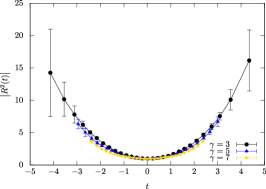
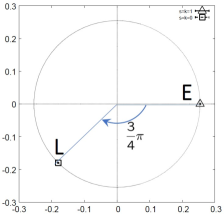
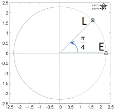
In Fig. 5 (Left), we plot in the complex plane for . Notice the chosen aspect ratio . For , the distribution of is close to the real axis, which suggests that one of the classical solutions represented by Hermitian dominates111111This can be understood theoretically by rescaling the matrices as , which brings the partition function into the form . Since appears only in the exponent, the path integral is dominated by some saddle-point configuration at large . at large . As becomes smaller, we observe that the distribution moves away from the real axis, but the flat region at both ends extends, suggesting the emergence of real time in that region121212This property can be understood as a result of classicalization due to the expanding space, which makes the action large at late times Kim:2011ts ; Kim:2012mw .. The result for is close to the Euclidean model, and it is qualitatively different from the results for .
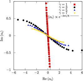
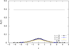
In order to see the properties of space, we consider
| (80) |
Note that defined in Eq. (50) is complex due to the complex weight in the partition function for the Lorentzian model (41). In particular, corresponds to real space, while corresponds to the Euclidean model. In Fig. 5 (Middle) and (Right), we plot and , respectively, against the time for . The block size used in defining in Eq. (66) and in Eq. (47) is chosen to be . From Fig. 5 (Middle), we find that space becomes real at late times, while the phase becomes slightly positive near . From Fig. 5 (Right), we find that the expanding behavior of is analogous to that observed for classical solutions Hatakeyama:2019jyw . Scaling behavior is observed for different values of , and decreasing results in extending the time direction, and making space more expanded at late times.
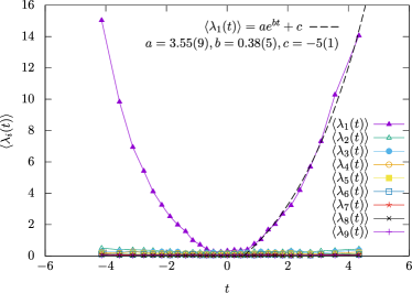

In Fig. 6 (Left), we show for , where are the eigenvalues of , the order parameter of the SSB of SO(9) symmetry defined in Eq. (49). We solve the ninth-order equation , where is the unit matrix, so that the coefficients maintain the holomorphicity with respect to . We observe that only one direction expands and the other directions remain small. The largest eigenvalue can be fitted nicely to an exponential function. In Fig. 6 (Right) we plot
| (81) |
against and for . We observe a clear band-diagonal structure with the off-diagonal elements being quite small, which is important in defining the submatrices (47). A similar behavior is observed for , which justifies our choice of the block size for in the present case. Such band-diagonal structure is not observed for .
5 Summary and outlook
In this article, we reviewed the progress in numerical studies on the type IIB matrix model. The numerical simulations of the Euclidean model using the factorization method and the CLM yield results that are consistent with the SSB of the SO(10) rotational symmetry to SO(3), in agreement with the GEM. While this is an interesting dynamical property, its relevance to the real world is unclear.
The Lorentzian version was studied first by using the approximation introduced to avoid the sign problem. This showed the exponential, followed by the power-law, expansion of three out of nine directions after a critical time. On the other hand, the obtained three-dimensional space was found to have a singular Pauli-matrix structure, which implies that the emergent space is not smooth.
This motivated the application of the CLM to the Lorentzian model. Without any cutoffs, the Lorentzian model was found to be equivalent to the Euclidean model, and that the emergent space-time obtained from the Lorentzian model should be interpreted as Euclidean.
To overcome this situation, we proposed to add a Lorentz-invariant mass term. Our preliminary results for the bosonic model are very promising. When the mass parameter is large enough, the path integral is dominated by one of the classical solutions, having Lorentzian signature and expanding behavior. As becomes smaller, the extent of the emergent time increases and the emergent space is expanding more at late times. The expansion at late times is consistent with an exponential behavior. The signature of space-time is Lorentzian at late times, while it seems to change to Euclidean at early times. We speculate that an expanding space-time with Lorentzian signature emerges at late times in the limit after taking the large– limit.
When space has an expanding behavior, we observe a clear block-diagonal structure, which is important in extracting the time-evolution from the matrix configurations that we obtain from the model. We also observe that space appears to be continuous instead of having the Pauli-matrix structure that was observed previously by using the approximation to avoid the sign problem.
In the bosonic model, we observed that only one out of nine spatial directions expands. This may be understood from the action of the original type IIB matrix model. Since the spatial directions expand exponentially, the term becomes dominant. The fluctuation of this term can be made small by having only one expanding direction.
As a future prospect, it is important to study the impact of the fermionic matrices on the dynamical generation of space-time. We expect supersymmetry to play an essential role in realizing the expansion of three spatial directions. It is known that vanishes if we set to zero except for two of them 9803117 ; 0003223 , which strongly suppresses the -dimensional space-time and possibly also -dimensional space-time considering the exponential expansion of space. As we have done in the Euclidean model, we have to introduce the fermionic mass term to avoid the singular drift problem in the CLM. It remains to be seen whether we can reduce the fermionic mass to the extent that enables us to see the effects of supersymmetry needed to make the space-time -dimensional.
Acknowledgements
T. A., K. H. and A. T. were supported in part by Grant-in-Aid (Nos. 17K05425, 19J10002, and 18K03614, 21K03532, respectively) from Japan Society for the Promotion of Science. This research was supported by MEXT as “Program for Promoting Researches on the Supercomputer Fugaku” (Simulation for basic science: from fundamental laws of particles to creation of nuclei, JPMXP1020200105) and JICFuS. This work used computational resources of supercomputer Fugaku provided by the RIKEN Center for Computational Science (Project ID: hp210165, hp220174), and Oakbridge-CX provided by the University of Tokyo (Project IDs: hp200106, hp200130, hp210094, hp220074) through the HPCI System Research Project. Numerical computation was also carried out on PC clusters in KEK Computing Research Center. This work was also supported by computational time granted by the Greek Research and Technology Network (GRNET) in the National HPC facility ARIS, under the project IDs SUSYMM and SUSYMM2. K. N. A and S. K. P. were supported in part by a Program of Basic Research PEVE 2020 (No. 65228700) of the National Technical University of Athens.
References
- (1) Ishibashi, N., Kawai, H., Kitazawa, Y., Tsuchiya, A.: A Large N reduced model as superstring. Nucl. Phys. B 498, 467–491 (1997) arXiv:hep-th/9612115. https://doi.org/10.1016/S0550-3213(97)00290-3
- (2) Aoki, H., Iso, S., Kawai, H., Kitazawa, Y., Tada, T.: Space-time structures from IIB matrix model. Prog. Theor. Phys. 99, 713–746 (1998) arXiv:hep-th/9802085. https://doi.org/10.1143/PTP.99.713
- (3) Hotta, T., Nishimura, J., Tsuchiya, A.: Dynamical aspects of large N reduced models. Nucl. Phys. B 545, 543–575 (1999) arXiv:hep-th/9811220. https://doi.org/10.1016/S0550-3213(99)00056-5
- (4) Ambjorn, J., Anagnostopoulos, K.N., Bietenholz, W., Hotta, T., Nishimura, J.: Large N dynamics of dimensionally reduced 4-D SU(N) superYang-Mills theory. JHEP 07, 013 (2000) arXiv:hep-th/0003208. https://doi.org/10.1088/1126-6708/2000/07/013
- (5) Ambjorn, J., Anagnostopoulos, K.N., Bietenholz, W., Hotta, T., Nishimura, J.: Monte Carlo studies of the IIB matrix model at large N. JHEP 07, 011 (2000) arXiv:hep-th/0005147. https://doi.org/10.1088/1126-6708/2000/07/011
- (6) Anagnostopoulos, K.N., Nishimura, J.: New approach to the complex action problem and its application to a nonperturbative study of superstring theory. Phys. Rev. D 66, 106008 (2002) arXiv:hep-th/0108041. https://doi.org/10.1103/PhysRevD.66.106008
- (7) Anagnostopoulos, K.N., Azuma, T., Nishimura, J.: A general approach to the sign problem: The factorization method with multiple observables. Phys. Rev. D 83, 054504 (2011) arXiv:1009.4504 [cond-mat.stat-mech]. https://doi.org/10.1103/PhysRevD.83.054504
- (8) Anagnostopoulos, K.N., Azuma, T., Nishimura, J.: A practical solution to the sign problem in a matrix model for dynamical compactification. JHEP 10, 126 (2011) arXiv:1108.1534 [hep-lat]. https://doi.org/10.1007/JHEP10(2011)126
- (9) Anagnostopoulos, K.N., Azuma, T., Nishimura, J.: Monte Carlo studies of the spontaneous rotational symmetry breaking in dimensionally reduced super Yang-Mills models. JHEP 11, 009 (2013) arXiv:1306.6135 [hep-th]. https://doi.org/%****␣IKKT_review-v14.bbl␣Line␣200␣****10.1007/JHEP11(2013)009
- (10) Anagnostopoulos, K.N., Azuma, T., Nishimura, J.: Monte Carlo studies of dynamical compactification of extra dimensions in a model of nonperturbative string theory. PoS LATTICE2015, 307 (2016) arXiv:1509.05079 [hep-lat]. https://doi.org/10.22323/1.251.0307
- (11) Anagnostopoulos, K.N., Azuma, T., Ito, Y., Nishimura, J., Papadoudis, S.K.: Complex Langevin analysis of the spontaneous symmetry breaking in dimensionally reduced super Yang-Mills models. JHEP 02, 151 (2018) arXiv:1712.07562 [hep-lat]. https://doi.org/10.1007/JHEP02(2018)151
- (12) Anagnostopoulos, K.N., Azuma, T., Ito, Y., Nishimura, J., Okubo, T., Kovalkov Papadoudis, S.: Complex Langevin analysis of the spontaneous breaking of 10D rotational symmetry in the Euclidean IKKT matrix model. JHEP 06, 069 (2020) arXiv:2002.07410 [hep-th]. https://doi.org/10.1007/JHEP06(2020)069
- (13) Krauth, W., Nicolai, H., Staudacher, M.: Monte Carlo approach to M theory. Phys. Lett. B 431, 31–41 (1998) arXiv:hep-th/9803117. https://doi.org/%****␣IKKT_review-v14.bbl␣Line␣275␣****10.1016/S0370-2693(98)00557-7
- (14) Austing, P., Wheater, J.F.: Convergent Yang-Mills matrix theories. JHEP 04, 019 (2001) arXiv:hep-th/0103159. https://doi.org/10.1088/1126-6708/2001/04/019
- (15) Nishimura, J., Vernizzi, G.: Spontaneous breakdown of Lorentz invariance in IIB matrix model. JHEP 04, 015 (2000) arXiv:hep-th/0003223. https://doi.org/10.1088/1126-6708/2000/04/015
- (16) Nishimura, J., Vernizzi, G.: Brane world from IIB matrices. Phys. Rev. Lett. 85, 4664–4667 (2000) arXiv:hep-th/0007022. https://doi.org/10.1103/PhysRevLett.85.4664
- (17) Ambjorn, J., Anagnostopoulos, K.N., Bietenholz, W., Hofheinz, F., Nishimura, J.: On the spontaneous breakdown of Lorentz symmetry in matrix models of superstrings. Phys. Rev. D 65, 086001 (2002) arXiv:hep-th/0104260. https://doi.org/10.1103/PhysRevD.65.086001
- (18) Aoyama, T., Nishimura, J., Okubo, T.: Spontaneous breaking of the rotational symmetry in dimensionally reduced super Yang-Mills models. Prog. Theor. Phys. 125, 537–563 (2011) arXiv:1007.0883 [hep-th]. https://doi.org/10.1143/PTP.125.537
- (19) Nishimura, J., Okubo, T., Sugino, F.: Systematic study of the SO(10) symmetry breaking vacua in the matrix model for type IIB superstrings. JHEP 10, 135 (2011) arXiv:1108.1293 [hep-th]. https://doi.org/%****␣IKKT_review-v14.bbl␣Line␣375␣****10.1007/JHEP10(2011)135
- (20) Kim, S.-W., Nishimura, J., Tsuchiya, A.: Expanding (3+1)-dimensional universe from a Lorentzian matrix model for superstring theory in (9+1)-dimensions. Phys. Rev. Lett. 108, 011601 (2012) arXiv:1108.1540 [hep-th]. https://doi.org/10.1103/PhysRevLett.108.011601
- (21) Ito, Y., Kim, S.-W., Koizuka, Y., Nishimura, J., Tsuchiya, A.: A renormalization group method for studying the early universe in the Lorentzian IIB matrix model. PTEP 2014(8), 083–01 (2014) arXiv:1312.5415 [hep-th]. https://doi.org/10.1093/ptep/ptu101
- (22) Ito, Y., Nishimura, J., Tsuchiya, A.: Power-law expansion of the Universe from the bosonic Lorentzian type IIB matrix model. JHEP 11, 070 (2015) arXiv:1506.04795 [hep-th]. https://doi.org/10.1007/JHEP11(2015)070
- (23) Aoki, T., Hirasawa, M., Ito, Y., Nishimura, J., Tsuchiya, A.: On the structure of the emergent 3d expanding space in the Lorentzian type IIB matrix model. PTEP 2019(9), 093–03 (2019) arXiv:1904.05914 [hep-th]. https://doi.org/10.1093/ptep/ptz092
- (24) Parisi, G.: On complex probabilities. Phys. Lett. B 131, 393–395 (1983). https://doi.org/10.1016/0370-2693(83)90525-7
- (25) Klauder, J.R.: Coherent State Langevin Equations for Canonical Quantum Systems With Applications to the Quantized Hall Effect. Phys. Rev. A 29, 2036–2047 (1984). https://doi.org/10.1103/PhysRevA.29.2036
- (26) Aarts, G., Seiler, E., Stamatescu, I.-O.: The Complex Langevin method: When can it be trusted? Phys. Rev. D 81, 054508 (2010) arXiv:0912.3360 [hep-lat]. https://doi.org/10.1103/PhysRevD.81.054508
- (27) Aarts, G., James, F.A., Seiler, E., Stamatescu, I.-O.: Complex Langevin: Etiology and Diagnostics of its Main Problem. Eur. Phys. J. C 71, 1756 (2011) arXiv:1101.3270 [hep-lat]. https://doi.org/10.1140/epjc/s10052-011-1756-5
- (28) Nishimura, J., Shimasaki, S.: New Insights into the Problem with a Singular Drift Term in the Complex Langevin Method. Phys. Rev. D 92(1), 011501 (2015) arXiv:1504.08359 [hep-lat]. https://doi.org/10.1103/PhysRevD.92.011501
- (29) Nagata, K., Nishimura, J., Shimasaki, S.: Argument for justification of the complex Langevin method and the condition for correct convergence. Phys. Rev. D 94(11), 114515 (2016) arXiv:1606.07627 [hep-lat]. https://doi.org/10.1103/PhysRevD.94.114515
- (30) Nishimura, J., Tsuchiya, A.: Complex Langevin analysis of the space-time structure in the Lorentzian type IIB matrix model. JHEP 06, 077 (2019) arXiv:1904.05919 [hep-th]. https://doi.org/10.1007/JHEP06(2019)077
- (31) Hatakeyama, K., Anagnostopoulos, K., Azuma, T., Hirasawa, M., Ito, Y., Nishimura, J., Papadoudis, S., Tsuchiya, A.: Complex Langevin studies of the emergent space-time in the type IIB matrix model (2022) arXiv:2201.13200 [hep-th]. https://doi.org/10.1142/9789811261633_0002
- (32) Nishimura, J.: Signature change of the emergent space-time in the IKKT matrix model (2022) arXiv:2205.04726 [hep-th]
- (33) Klinkhamer, F.R.: IIB matrix model and regularized big bang. PTEP 2021(6), 063 (2021) arXiv:2009.06525 [hep-th]. https://doi.org/10.1093/ptep/ptab059
- (34) Brahma, S., Brandenberger, R., Laliberte, S.: Emergent cosmology from matrix theory. JHEP 03, 067 (2022) arXiv:2107.11512 [hep-th]. https://doi.org/10.1007/JHEP03(2022)067
- (35) Steinacker, H.C.: Gravity as a quantum effect on quantum space-time. Phys. Lett. B 827, 136946 (2022) arXiv:2110.03936 [hep-th]. https://doi.org/10.1016/j.physletb.2022.136946
- (36) Brahma, S., Brandenberger, R., Laliberte, S.: Emergent Metric Space-Time from Matrix Theory (2022) arXiv:2206.12468 [hep-th]
- (37) Battista, E., Steinacker, H.C.: On the propagation across the big bounce in an open quantum FLRW cosmology (2022) arXiv:2207.01295 [gr-qc]
- (38) Karczmarek, J.L., Steinacker, H.C.: Cosmic time evolution and propagator from a Yang-Mills matrix model (2022) arXiv:2207.00399 [hep-th]
- (39) Aoki, H., Iso, S., Kawai, H., Kitazawa, Y., Tsuchiya, A., Tada, T.: IIB matrix model. Prog. Theor. Phys. Suppl. 134, 47–83 (1999) arXiv:hep-th/9908038. https://doi.org/10.1143/PTPS.134.47
- (40) Nishimura, J.: Lattice superstring and noncommutative geometry. Nucl. Phys. B Proc. Suppl. 129, 121–134 (2004) arXiv:hep-lat/0310019. https://doi.org/10.1016/S0920-5632(03)02513-1
- (41) Azuma, T.: Matrix models and the gravitational interaction (2004) arXiv:hep-th/0401120
- (42) Steinacker, H.: Emergent Geometry and Gravity from Matrix Models: an Introduction. Class. Quant. Grav. 27, 133001 (2010) arXiv:1003.4134 [hep-th]. https://doi.org/10.1088/0264-9381/27/13/133001
- (43) Nishimura, J.: The Origin of space-time as seen from matrix model simulations. PTEP 2012, 01–101 (2012) arXiv:1205.6870 [hep-lat]. https://doi.org/10.1093/ptep/pts004
- (44) Nishimura, J.: Recent developments in the type IIB matrix model. Fortsch. Phys. 62, 754–764 (2014) arXiv:1405.5904 [hep-th]. https://doi.org/10.1002/prop.201400040
- (45) Ydri, B.: Review of M(atrix)-Theory, Type IIB Matrix Model and Matrix String Theory (2017) arXiv:1708.00734 [hep-th]
- (46) Nishimura, J.: New perspectives on the emergence of (3+1)D expanding space-time in the Lorentzian type IIB matrix model. PoS CORFU2019, 178 (2020) arXiv:2006.00768 [hep-lat]. https://doi.org/10.22323/1.376.0178
- (47) Schild, A.: Classical Null Strings. Phys. Rev. D 16, 1722 (1977). https://doi.org/10.1103/PhysRevD.16.1722
- (48) Fukuma, M., Kawai, H., Kitazawa, Y., Tsuchiya, A.: String field theory from IIB matrix model. Nucl. Phys. B 510, 158–174 (1998) arXiv:hep-th/9705128. https://doi.org/%****␣IKKT_review-v14.bbl␣Line␣825␣****10.1016/S0550-3213(97)00584-1
- (49) Anagnostopoulos, K.N., Bietenholz, W., Nishimura, J.: The Area law in matrix models for large N QCD strings. Int. J. Mod. Phys. C 13, 555–564 (2002) arXiv:hep-lat/0112035. https://doi.org/10.1142/S0129183102003334
- (50) Ambjorn, J., Anagnostopoulos, K.N., Nishimura, J., Verbaarschot, J.J.M.: The Factorization method for systems with a complex action: A Test in random matrix theory for finite density QCD. JHEP 10, 062 (2002) arXiv:hep-lat/0208025. https://doi.org/10.1088/1126-6708/2002/10/062
- (51) Azcoiti, V., Di Carlo, G., Galante, A., Laliena, V.: New proposal for numerical simulations of theta vacuum - like systems. Phys. Rev. Lett. 89, 141601 (2002) arXiv:hep-lat/0203017. https://doi.org/10.1103/PhysRevLett.89.141601
- (52) Fodor, Z., Katz, S.D.: Critical point of QCD at finite T and mu, lattice results for physical quark masses. JHEP 04, 050 (2004) arXiv:hep-lat/0402006. https://doi.org/10.1088/1126-6708/2004/04/050
- (53) Ambjorn, J., Anagnostopoulos, K.N., Nishimura, J., Verbaarschot, J.J.M.: Noncommutativity of the zero chemical potential limit and the thermodynamic limit in finite density systems. Phys. Rev. D 70, 035010 (2004) arXiv:hep-lat/0402031. https://doi.org/10.1103/PhysRevD.70.035010
- (54) Clark, M.A., Kennedy, A.D.: The RHMC algorithm for two flavors of dynamical staggered fermions. Nucl. Phys. B Proc. Suppl. 129, 850–852 (2004) arXiv:hep-lat/0309084. https://doi.org/10.1016/S0920-5632(03)02732-4
- (55) Batrouni, G.G., Katz, G.R., Kronfeld, A.S., Lepage, G.P., Svetitsky, B., Wilson, K.G.: Langevin Simulations of Lattice Field Theories. Phys. Rev. D 32, 2736 (1985). https://doi.org/10.1103/PhysRevD.32.2736
- (56) Seiler, E., Sexty, D., Stamatescu, I.-O.: Gauge cooling in complex Langevin for QCD with heavy quarks. Phys. Lett. B 723, 213–216 (2013) arXiv:1211.3709 [hep-lat]. https://doi.org/10.1016/j.physletb.2013.04.062
- (57) Nagata, K., Nishimura, J., Shimasaki, S.: Justification of the complex Langevin method with the gauge cooling procedure. PTEP 2016(1), 013–01 (2016) arXiv:1508.02377 [hep-lat]. https://doi.org/10.1093/ptep/ptv173
- (58) Ito, Y., Nishimura, J.: The complex Langevin analysis of spontaneous symmetry breaking induced by complex fermion determinant. JHEP 12, 009 (2016) arXiv:1609.04501 [hep-lat]. https://doi.org/10.1007/JHEP12(2016)009
- (59) Hatakeyama, K., Matsumoto, A., Nishimura, J., Tsuchiya, A., Yosprakob, A.: The emergence of expanding space–time and intersecting D-branes from classical solutions in the Lorentzian type IIB matrix model. PTEP 2020(4), 043–10 (2020) arXiv:1911.08132 [hep-th]. https://doi.org/10.1093/ptep/ptaa042
- (60) Fukugita, M., Oyanagi, Y., Ukawa, A.: Langevin Simulation of the Full QCD Hadron Mass Spectrum on a Lattice. Phys. Rev. D 36, 824 (1987). https://doi.org/10.1103/PhysRevD.36.824
- (61) Attanasio, F., Jäger, B.: Dynamical stabilisation of complex Langevin simulations of QCD. Eur. Phys. J. C 79(1), 16 (2019) arXiv:1808.04400 [hep-lat]. https://doi.org/10.1140/epjc/s10052-018-6512-7
- (62) Kim, S.-W., Nishimura, J., Tsuchiya, A.: Expanding universe as a classical solution in the Lorentzian matrix model for nonperturbative superstring theory. Phys. Rev. D 86, 027901 (2012) arXiv:1110.4803 [hep-th]. https://doi.org/10.1103/PhysRevD.86.027901
- (63) Kim, S.-W., Nishimura, J., Tsuchiya, A.: Late time behaviors of the expanding universe in the IIB matrix model. JHEP 10, 147 (2012) arXiv:1208.0711 [hep-th]. https://doi.org/10.1007/JHEP10(2012)147