Space-fluid Adaptive Sampling by Self-Organisation

Abstract.

A recurrent task in coordinated systems is managing (estimating, predicting, or controlling) signals that vary in space, such as distributed sensed data or computation outcomes. Especially in large-scale settings, the problem can be addressed through decentralised and situated computing systems: nodes can locally sense, process, and act upon signals, and coordinate with neighbours to implement collective strategies. Accordingly, in this work we devise distributed coordination strategies for the estimation of a spatial phenomenon through collaborative adaptive sampling. Our design is based on the idea of dynamically partitioning space into regions that compete and grow/shrink to provide accurate aggregate sampling. Such regions hence define a sort of virtualised space that is “fluid”, since its structure adapts in response to pressure forces exerted by the underlying phenomenon. We provide an adaptive sampling algorithm in the field-based coordination framework, and prove it is self-stabilising and locally optimal. Finally, we verify by simulation that the proposed algorithm effectively carries out a spatially adaptive sampling while maintaining a tuneable trade-off between accuracy and efficiency.

1. Introduction

A significant problem in computer systems engineering is dealing with phenomena that vary in space: for instance, their estimation, prediction, and control. Concrete related application examples include: the monitoring of waste in urban areas to improve waste gathering strategies [imran2019smart-waste]; the estimation of pollution in a geographical area, for alerting or mitigation-aimed response purposes [casadei2020pulverization]; the sensing of the temperature in a large building, to support the synthesis of control policies for the Heating, Ventilation, and Air Conditioning (HVAC) system [Manjarres2017hvac-predictive-control]. The general solution for addressing this kind of problem consists of deploying a set of sensors and actuators in space, and building a distributed system that processes gathered data and possibly determines a suitable actuation in response [DBLP:journals/percom/WuKT11]. In many settings, the computational activity can (or has to) be performed in-network [DBLP:journals/wc/FasoloRWZ07] in a decentralised way: in such systems, nodes locally sense, process, and act upon the environment, and coordinate with neighbour nodes to collectively self-organise their activity. However, in general there exists a trade-off between performance and efficiency, that suggests concentrating the activities on few nodes, or to endow systems with the capability of autonomously adapt the granularity of computation [DBLP:journals/tcyb/YaoVP13].

In this work, we focus on sampling signals that vary in space. Specifically, we would like to sample a spatially distributed signal through device coordination and self-organisation such that the samples accurately reflect the original signal and the least amount of resources is used to do so. In particular, we push forward a vision of space-fluid computations, namely computations that are fluid, i.e. change seamlessly, in space and – like fluids – adapt in response to pressure forces exerted by the underlying phenomenon. We reify the vision through an algorithm that handles the shape and lifetime of leader-based “regional processes” (cf. [FGCS2020-scr]), growing/shrinking as needed to sample a phenomenon of interest with a (locally) maximum level of accuracy and minimum resource usage. For instance, we would like to sample more densely those regions of space where the spatial phenomenon under observation has high variance, to better reflect its spatial dynamics. On the contrary, in regions where variance is low, we would like to sample the phenomenon more sparsely to, e.g., save energy, communication bandwidth, etc. while preserving the same level of accuracy.

Accordingly, we consider the field-based coordination framework of aggregate computing [BealIEEEComputer2015, JLAMP2019], which has proven to be effective in modelling and programming self-organising behaviour in situated networks of devices interacting asynchronously. On top of it, we devise a solution that we call aggregate sampling, inspired by the approaches of self-stabilisation [TOMACS2018] and density-independence [TAAS2017], that maps an input field representing a signal to be sampled into a regional partition field where each region provides a single sample; then, we characterise the aggregate sampling error based on a distance defined between stable snapshots of regional partition fields, and propose that an effective aggregate sampling is one that is locally optimal w.r.t. an error threshold, meaning that the regional partition cannot be improved simply by merging regions. In summary, we provide the following contributions:

• we define a model for distributed collaborative adaptive sampling and characterise the corresponding problem in the field-based coordination framework;

• we implement an algorithmic solution to the problem that leverages self-organisation patterns like gradients [DBLP:journals/nc/Fernandez-MarquezSMVA13, TOMACS2018] and coordination regions [FGCS2020-scr];

• we prove this algorithm to self-stabilise, and to actually provide an effective sampling according to a definition of “locally optimal regional partition”;

• we experimentally validate the algorithm to verify interesting trade-offs between sparseness of the sampling and its error.

This manuscript is an extended version of the conference paper [DBLP:conf/coordination/CasadeiMPVZ22], providing (i) a more extensive and detailed coverage of related work; (ii) more examples, clarifications, and details regarding the formal model; (iii) a discussion of the source code of the aggregate computing implementation; and (iv) proofs of self-stabilisation and local optimality of the proposed algorithm.

The rest of the paper is organised as follows. Section 2 covers motivation and related work. Section 3 provides a model for distributed sampling and the problem statement. Section 4 describes an algorithmic solution to the problem of sampling a distributed signal using the framework of aggregate computing. LABEL:s:eval performs an experimental validation of the proposed approach. Finally, LABEL:s:conc provides conclusive thoughts and delineates directions for further research.

2. Motivation and Related Work

2.1. Motivations, Goal, and Applications

Consider a Wireless Sensor Network (WSN) of any topology, statically (i.e. design-time, no mobility) deployed across a geographical area to monitor a spatially-distributed phenomenon, such as, for instance, air quality, as depicted in Figure 1.

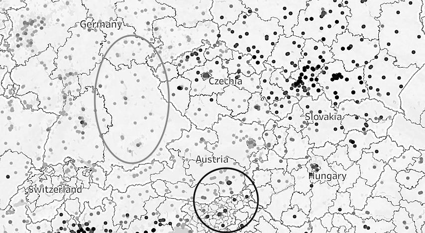
Figure 1. Air quality statistics map taken from https://archive.ph/dMJO2. There are areas where the underlying phenomenon does not vary significantly in space (light-grey oval), hence sampling could be made sparser with tolerable loss of accuracy. In others (darker circle), variance is high, requiring a more detailed spatial sampling.

We want to dynamically (at run-time) and adaptively (depending on the phenomenon itself) find a sparse set of samplers, i.e., devices responsible for providing sensing data regarding some underlying phenomenon. We want the selection of samplers to depend on both the spatial distribution of devices and the input phenomenon. Therefore, the idea is that each sampler is responsible for an exclusive spatial sampling region that may include several other devices, i.e., a partition of the system/environment. Moreover, we want to determine a partitioning of the connected sampling devices that minimises the number and maximises the size of sampling regions, while preserving as much as possible the underlying information. Hence, in areas with low variance amongst spatially distributed samples’ values, we want our regions to be larger, as many samples will report similar values, and hence one sample nicely represents all. Conversely, in areas with high spatial variance between samples, smaller regions are necessary as even proximal samples may have very different values, hence more samples are required to accurately represent the phenomenon. We also consider large-scale deployments with hundreds or thousands of devices.

Accordingly, we aim at designing a decentralised algorithm that can:

• dynamically (at run-time, continuously) partition a set of sampling devices into sampling regions;

• consider phenomenon-specific metrics (e.g. variance of the sensors’ readings) for deciding how to (re)compute partitions;

• both up-scale and down-scale sampling depending on such metrics;

• do so in a fully distributed way, based solely on local interactions (i.e., within a 1-hop neighbourhood).

A similar algorithm can provide benefits across multiple application domains, as also witnessed by the below described related literature. All forms of environmental monitoring can greatly benefit, for instance, as many phenomena in such a domain are inherently spatially distributed: air quality, water pollution, soil radiation, landslide monitoring, crop growth, and so on [Cox99RiskAnalysis, YOO2020117091, DBLP:conf/lcn/ZamanGMB14, DBLP:journals/ejwcn/MysorewalaCP12]. Another field of application is ecological monitoring, such as geolocation of wolf packs or other animals moving habits [DBLP:journals/sac/PeyrardSSBN13]. But in general, any application whose goal is to monitoring any measurable phenomenon, with unknown or uncertain spatial dynamics, may find benefits in our proposed approach.

2.2. Related Work on Adaptive Spatial Sampling

There are several approaches in the literature that attempt to solve this and similar problems, with heterogeneous techniques, that we collectively refer to under the umbrella term of “adaptive spatial sampling”. Amongst these, some [DBLP:journals/corr/abs-1811-01303, doi:10.1080/01621459.1990.10474975] are restricted to the so-called sampling design problem, that is, their concern is to deliver either design-time decision support about where to deploy sensor devices or analytically devise out the best sampling algorithm given domain expertise or infrastructural requirements (most often, residual energy management). Our approach is not directly comparable to these, as we are concerned with run-time adaptation of the sampling process based on domain-specific properties (e.g. sampling variance, that depends on the phenomenon under observation). Others [DBLP:conf/iros/RahimiHKSE05, DBLP:conf/rss/GargA14, DBLP:journals/corr/abs-2105-10018, DBLP:journals/iet-wss/HamoudaP11, DBLP:conf/cdc/GrahamC09] more closely pursue our goal, but assume mobile sensing devices (e.g. robots), hence are concerned with how to move them at run-time to optimise some desired metric (e.g. sampling accuracy). On the contrary, we assume static sensor devices that have been already deployed on a target area, without any prior knowledge of the actual spatial distribution of the phenomenon to observe. Finally, a great deal of related research contributions have the fundamental difference of adapting the sampling process to domain-agnostic, infrastructural properties such as residual energy, distance amongst devices, bandwidth consumption, rather than on the specific spatial distribution (and dynamics) of the phenomenon under monitoring [DBLP:conf/infocom/YounisF04, DBLP:journals/adhoc/MhatreR04, DBLP:journals/cn/BandyopadhyayC04, DBLP:conf/infocom/BandyopadhyayC03, DBLP:journals/wc/SohrabiGAP00, DBLP:journals/pieee/StankovicALSH03, DBLP:conf/infocom/BhardwajC02, DBLP:journals/tac/OgrenFL04].

Narrowing down the research landscape just overviewed, we now describe and compare in more detail the approaches to spatial adaptive sampling most similar to ours, emphasising the most notable differences.

In reference [DBLP:conf/mass/VirrankoskiS05] the Topology Adaptive Spatial Clustering algorithm is presented. It is a distributed algorithm that partitions a WSN into a set of disjoint sampling clusters, with no prior knowledge of cluster number or size (like ours), by encoding geographical distance, connectivity, and deployment density information in a single measure upon which leader election (for cluster heads) happens. The goal is to group together nodes in proximity and within regions of similar deployment density, to improve efficiency of data aggregation and compression. Besides the focus on efficiency, that is only half the story in our approach (the other being accuracy, hence the trade-off), two are the fundamental differences our approach has with respect to this: first, in our case adaptation is domain dependent, in the sense that it depends on some property (e.g. variance) of the phenomenon under observation, not on infrastructural properties; second, we do also consider over-sampling when variation is high, whereas reference [DBLP:conf/mass/VirrankoskiS05] only considers under-sampling where measures are redundant.

In reference [DBLP:conf/aina/LiuXZWL13], another distributed approach to spatial adaptive sampling is presented. It is based on the assumption that neighbouring sampling nodes usually have similar readings (high spatial correlation), hence can be grouped in a cluster to improve energy consumption. The proposed algorithm uses such spatial correlation, two application-specific threshold parameters (error tolerance and correlation range), and residual energy to elect cluster heads, with the goal of minimising the number of clusters, and the variance of their size. The introduction of the two application-dependant parameters makes this proposal closer to ours, as they could be used to steer the adaptation toward domain-specific aspects, to some extent. However, most of the calculations still rely on infrastructural properties rather than measures about the phenomenon of interest, and the focus is, once again, on energy saving, thus, authors do not consider over-sampling but solely under-sampling.

Reference [DBLP:conf/ccnc/LinM07] shares with us the interest in performing adaptation based on the information observed by sensors, rather than on network, energy, or other infrastructural aspects. However, they consider a special case where the clusters must correspond to pre-determined “sources of interest”, such as physical objects/devices in the environment. Moreover, clusters are formed with the secondary objective of being balanced, whereas we allow them to be of different sizes and shapes (and even encourage to be so depending on the spatial distribution of the phenomenon of interest).

Reference [DBLP:conf/icac/LeeVP11] proposes SILENCE, a distributed, space-time adaptive sampling algorithm based on (space-time) correlation of measured values. The foremost goal pursued is efficiency: SILENCE in fact strives to minimise communication and processing overhead, by minimising sampling redundancy and also adapting (i.e. slowing down) the scheduling speed of sensor devices. However, yet again the basic assumption, and focus of the approach, is the case where spatial correlation of sampled values is high; whereas we explicitly focus on the opposite situation (while still providing a working solution even in the case considered by SILENCE). Furthermore, also SILENCE only considers down-sampling.

Finally, the ASample algorithm [DBLP:conf/sutc/SzczytowskiKS10] is the one approach most similar to ours, not in the techniques exploited, but in pursuing domain-driven adaptation, in doing so in a fully-distributed way, and in considering the opportunity to over-sample, too. In particular, ASample builds a Voronoi tessellation of the area where the WSN is deployed, in a fully distributed way by considering only neighbourhood information, instead of the whole topology. Such a tessellation considers a desired sampling accuracy, specified at the application level: while a given Voronoi region is within the accuracy bound, it keeps expanding; on the contrary, whenever the accuracy constraint is violated, a virtual centroid of a novel Voronoi region is spawned, with a value that is obtained through interpolation of the neighbouring regions. This is an important aspect to consider, as it introduces synthetic data, which is something we avoid as we only increase sampling granularity if there are actual devices available in the target area. Moreover, there is an assumption underlying the ASample approach that does not hold in general, and, specifically, it is in contrast with our intended goal (obtaining potentially irregular clusters to reflect the irregular spatial distribution of the observed phenomenon): it is assumed that the smaller the area covered by the Voronoi region, the less representative the samples drawn are, hence the smaller the impact on the global sampling accuracy. In our targeted scenarios, the opposite could be true, too: smaller regions represent sharp variance of measurements across space, and more accurately represent the irregularities of the underlying phenomenon.

3. Distributed Aggregate Sampling: Model

In order to define the problem and characterise our approach, we leverage the event structure framework [DBLP:journals/tcs/NielsenPW81, ABDV-COORDINATION2018], which provides a general model of situated computations. Within this formal framework, in this section we describe the computational model (Section 3.1), self-stabilisation as a desired property of solutions in this model (Section 3.2), and the spatial sampling problem that we tackle in this manuscript (Section 3.3). The computational model introduces the necessary terminology to understand both the problem formulation and the solution we propose in Section 4. Introducing the self-stabilisation property is required to be able to evaluate such a solution in its effort to adapt to the dynamics of the phenomenon of interest, both formally as done in Section 4.3 and practically as done later in LABEL:s:eval.

3.1. Computational Model

We consider a computational model where a set of devices (typically comprising sensors and actuators to perceive and act upon the environment) compute at discrete steps called computation rounds and interact with neighbour devices by exchanging messages. Executions of such systems can be modelled through event structures [DBLP:journals/tcs/NielsenPW81, DBLP:journals/ijpp/Pratt86] as in [TOCL2019, ABDV-COORDINATION2018]. Following the general approach in [ABDV-COORDINATION2018], we enrich the event structure with information about the devices where events occur.

[Situated event structure] A situated event structure (ES) is a triplet ${\langle E,\rightsquigarrow,d\rangle}$ where:

• $E$ is a countable set of events;

• $\rightsquigarrow\;\subseteq E\times E$ is a messaging relation from a sender event to a receiver event (these are also called neighbour events);

• $d:E\to\Delta$, where $\Delta$ is a finite set of device identifiers $\delta_{i}$, maps an event $\epsilon\in E$ to the device $d(\epsilon)\in\Delta$ where the event takes place.

The elements of the triplet are such that:

• the transitive closure of $\rightsquigarrow$ forms an irreflexive partial order $<\;\subseteq E\times E$, called causality relation (an event $\epsilon$ is in the past of another event $\epsilon^{\prime}$ if $\epsilon<\epsilon^{\prime}$, in the future if $\epsilon^{\prime}<\epsilon$, or concurrent otherwise);

• for any $\delta\in\Delta$, the projection of the ES to the set of events $E_{\delta}={\left\{\epsilon\in E~{}\mid~{}d(\epsilon)=\delta\right\}}$ forms a well-order, i.e., a sequence $\epsilon_{0}\rightsquigarrow\epsilon_{1}\rightsquigarrow\epsilon_{2}\rightsquigarrow\dots$.

Additionally, we introduce the following notation:

• $\mathit{recvs}(\epsilon)=\{d(\epsilon^{\prime})\mid\epsilon~{}\rightsquigarrow~{}\epsilon^{\prime}\}$ to denote the set of receivers of $\epsilon$, i.e., the devices receiving a message from $\epsilon$;

• $T_{\epsilon_{0}}^{-}=\{\epsilon:\epsilon<\epsilon_{0}\}$ to denote the past event cone of $\epsilon_{0}$ (which is a finite set, since we assume the system has a starting point in time at any device);

• $T_{\epsilon_{0}}^{+}=\{\epsilon:\epsilon_{0}<\epsilon\}$ to denote the future event cone of $\epsilon_{0}$;

• $X|_{E^{\prime}}$ to denote the projection of a set, function, or ES $X$ to the set of events $E^{\prime}\subseteq E$. Note that the projection of an event structure to the future event cone of an event is still a well-formed ES.

Figure 2. Example of an event structure. In the node labels, superscripts denote device identifiers, while subscripts are progressive numbers denoting subsequent rounds at the same device. The blue (resp. green) background denotes the future (resp. past) of a reference event denoted with a yellow background.

An example of ES is given in Figure 2, events denote computation rounds. Notice that self-messages (i.e., messages from an event to the next on the same device) can be used to model persistence of state over time. Also, notice that two subsequent events at some device (e.g., $\epsilon_{4}^{4}$ and $\epsilon_{5}^{4}$ of device $4$ in Figure 2) may share a same sender event from a neighbour ($\epsilon_{2}^{3}$ in this case): in a real system, this could be due to two distinct communication acts with the same message, as well as to a mechanism by which the receiving device reuses the most recently received message from that neighbour through some message retention policy (which is an implementation mechanism useful to support stability of neighbourhoods).

Remark 1 (Communication and distributed execution).

The description of a system execution as an event structure as per Definition 3.1 abstracts from details regarding the actual communication and scheduling mechanisms used in a deployed system. Concrete communication mechanisms may include point-to-point network channels, based on wired or wireless technologies, broadcasts, intermediaries (like, e.g., the cloud), or even stigmergic (i.e., environment-mediated) means. The computation rounds may be scheduled at a fixed frequency, using a particular time distribution, or reactively (e.g., in response to new sensor values or reception of messages from neighbours). A more in-depth discussion of how aggregate computing systems may be deployed and executed can be found in [casadei2020pulverization, lmcs-timefluid].

In the computation model we consider, based on [ABDV-COORDINATION2018], each event $\epsilon$ represents the execution of a program taking all incoming messages, and producing an outgoing message (sent to all neighbours) and a result value associated with $\epsilon$. Such “map” of result values across all events defines a computational field, as follows.

[Computational field] Let $\mathbf{E}={\langle E,\rightsquigarrow,d\rangle}$ be an event structure. A computational field on $\mathbf{E}$ is a function $f:E\to\mathbb{V}$ that maps every event $\epsilon$ in $E$ (also called the domain of the field) to some value in a value set $\mathbb{V}$. Computational fields are essentially the “distributed values” which our model deals with; hence computation is captured by the following definition.

[Field computation] Let $\mathbf{E}={\langle E,\rightsquigarrow,d\rangle}$ be an event structure, and denote $\mathbb{F}_{E,\mathbb{V}}$ the set of fields on domain $E$ and co-domain $\mathbb{V}$, i.e., $\mathbb{F}_{E,\mathbb{V}}=\{f:E\to\mathbb{V}\}$. Given two sets of values $\mathbb{V},\mathbb{V}^{\prime}$, a field computation over $\mathbf{E}$ is a function $\Phi_{\mathbf{E}}:\mathbb{F}_{E,\mathbb{V}}\to\mathbb{F}_{E,\mathbb{V}^{\prime}}$ mapping an input field to an output field on the same domain of $\mathbf{E}$ (but possibly on a different co-domain). This definition naturally extends to the case of zero or multiple input fields.

Now, we define the notion of a field-based program, which we denote as a construct expressing a computation on any possible environment, where an environment can be modelled by an event structure and fields over it denoting environmental values perceivable by devices (e.g., temperature fields would assign a temperature value to each event).

[Field-based operator] A field-based operator (or field-based program) is a function $P$ taking an event structure as input and yielding the field computation that would occur on it, namely $P(\mathbf{E})=\Phi_{\mathbf{E}}$.

In other words, a field-based operator works as a “program” (design-time): it applies to a certain event structure to generate a resulting field computation (run-time). It would also be correct to say that a field-based program provides an implementation of a field-based operator, similarly to how, e.g., quick-sort provides an implementation of a sorting operator on lists. Notice also that we restrict our analysis to computable field-based operators as per previous work [ABDV-COORDINATION2018].

There exist core languages and full-fledged programming languages for conveniently expressing field-based programs: these are known as field calculi and aggregate programming languages, respectively [JLAMP2019]. One of these is used in Section 4.2 to implement our adaptive spatial sampling algorithm. However, as the following example demonstrates, field-based programs can also be expressed, in our framework of event structures, by a local perspective, in terms of how inputs and ingoing messages at one event are mapped to an output and outgoing messages.

[Gradient field computation and operator] Term gradient commonly refers to a kind of distributed data structures for estimating the distance from any device in a network to its closest source device, and a family of distributed algorithms for building them [audrito2017ult], which are very useful for implementing self-organising systems [Nagpal2002programmable-self-assembly, TOMACS2018, DBLP:conf/saso/WolfH07].

In our framework, a distributed algorithm for building gradients (gradient operator) can be modelled as a field-based operator $P_{G}$ mapping any event structure $\mathbf{E}={\langle E,\rightsquigarrow,d\rangle}$ to a gradient field computation $\Phi_{G}$ over it. A gradient field computation $\Phi_{G}:\mathbb{F}_{\mathbf{E},\mathit{Bool}\times\mathit{Metric}}\to\mathbb{F}_{\mathbf{E},\mathbb{R}}$ is essentially a map:

• from an input field $f_{i}:\mathbb{F}_{\mathbf{E},\mathit{Bool}\times\mathit{Metric}}$ mapping each event $\epsilon\in E$ with a pair $(\mathit{source},\mathit{metric})\in\mathit{Bool}\times\mathit{Metric}$, where $\mathit{Metric}\subseteq E\times\mathbb{R}$, denoting source events/devices (those where $\mathit{source}=\top$), distinguished from non-source events/devices (those where $\mathit{source}=\bot$), and a metric associating neighbouring events to an estimation of the corresponding spatial distance, $\mathit{metric}(\epsilon)=\{(\epsilon^{\prime},x)\mid\epsilon^{\prime}\rightsquigarrow\epsilon\land x\in\mathbb{R}\}$;

• to the output field stabilising (cf. Section 3.2) to the minimum distances to source devices.

A simple operator for a gradient computation could be implemented through the following function, local to an event $\epsilon_{0}\in E$ receiving from a possibly empty set of sender events $\epsilon_{i}$ (with $\epsilon_{0}$ denoting the sender event at the same device, if any, and with $\epsilon_{i>0}$ the sender events from other devices), of the input field’s value and the message set $\mathcal{M}=\{\epsilon_{i}\mapsto g_{i}\}$ providing the neighbours’ current gradient estimates:

$$g(\mathit{source},\{\epsilon_{i}\mapsto\mathit{dist}_{i}\},\{\epsilon_{i}\mapsto g_{i}\})=\begin{cases}0&\mathit{source}=\top\\ \min_{i>0}\{g_{i}+dist_{i}\}&\mathit{source}=\bot\land\{\epsilon_{i>0}\}\neq\emptyset\\ +\infty&\text{otherwise}\end{cases}$$

An example of the induced computation is shown in Figure 3, assuming a simple metric where $\mathit{dist}_{0}=0$ and $\mathit{dist}_{i>0}=1$.

3.2. Self-stabilisation

We now provide the definitions necessary to model self-stabilisation following the approach in [TOMACS2018]. Namely, the following definitions capture the idea of adaptiveness whereby as the environment of computation stabilises, then the result of computation stabilises too, and such a result does not depend on previous transitory changes.

[Static environment] An event structure $\mathbf{E}={\langle E,\rightsquigarrow,d\rangle}$ is said to be a static environment if it has stable topology, namely all events of a given device always share the same set of receivers, i.e., $\forall\epsilon,\epsilon^{\prime},d(\epsilon)=d(\epsilon^{\prime})\Rightarrow\mathit{recvs}(\epsilon)=\mathit{recvs}(\epsilon^{\prime})$.

Note that, following the approach in [TOMACS2018], we introduce the notion of a static environment to capture the eventual situation in which the environment stops perturbing the system. This is instrumental to rely on an abstract characterisation of self-stabilising computations, which are those in which the system keeps intercepting changes in the environment and adapting to them: whenever (and if) the environment becomes static, one can observe the result of that adaptation that eventually establishes.

[Stabilising environment] An event structure $\mathbf{E}={\langle E,\rightsquigarrow,d\rangle}$ is said to be a stabilising environment if it is eventually static, i.e., $\exists\epsilon_{0}\in E\textrm{~{}such that~{}}\mathbf{E}|_{T_{\epsilon_{0}}^{+}}={\langle E|_{T_{\epsilon_{0}}^{+}},\rightsquigarrow|_{T_{\epsilon_{0}}^{+}},d|_{T_{\epsilon_{0}}^{+}}\rangle}$ is static. In this case we say it is static since event $\epsilon_{0}$.

[Stabilising field] Let event structure $\mathbf{E}={\langle E,\rightsquigarrow,d\rangle}$ be a stabilising environment, static since event $\epsilon_{0}$. A field $f:E\to\mathbb{V}$ is said stabilising if it eventually provides stable output (an output that does not change since some round), i.e., $\exists\epsilon>\epsilon_{0}\textrm{~{}such that~{}}\forall\epsilon^{\prime}>\epsilon,\epsilon^{\prime\prime}>\epsilon\textrm{~{}it holds that~{}}d(\epsilon^{\prime})=d(\epsilon^{\prime\prime})\implies f(\epsilon^{\prime})=f(\epsilon^{\prime\prime})$.

An example of a stabilising field, which can also be thought as being generated by a gradient computation (cf. 1), is provided in Figure 3. The environment is static since event $\epsilon_{1}^{3}$ (every event in the future event cone of $\epsilon_{1}^{3}$ has the same set of receivers), and from event $\epsilon_{2}^{3}$ (excluded) it holds that each device does not change the value it produces in its rounds.

Figure 3. Example of a stabilising field. We use labels above the nodes to denote the values computed in the corresponding events, assuming the program is a gradient operator as per 1.

[Stabilising computation] A field computation $\Phi_{\mathbf{E}}=\mathbb{F}_{E,\mathbb{V}}\to\mathbb{F}_{E,\mathbb{V}}$ is said stabilising if, when applied to a stabilising input field, it yields a stabilising output field.

[Self-stabilising operator] A field-based operator (or program) $P$ is said self-stabilising, if in any stabilising environment $\mathbf{E}$ it yields a stabilising computation $\Phi_{\mathbf{E}}$ such that, for any pair of input fields $f_{1},f_{2}$ eventually equal, i.e. $f_{1}|_{T_{\epsilon}^{+}}=f_{2}|_{T_{\epsilon}^{+}}$ for some event $\epsilon$, their output is eventually equal too, i.e., there exists a $\epsilon^{\prime}>\epsilon$ such that $\Phi_{\mathbf{E}}(f_{1})|_{T_{\epsilon^{\prime}}^{+}}=\Phi_{\mathbf{E}}(f_{2})|_{T_{\epsilon^{\prime}}^{+}}$

Notice that universally quantifying over event structures, i.e., considering infinitely many system executions, makes finding decision procedures for properties like stabilisation undecidable in general. However, this does not prevent us from reasoning about such properties for a specific program, as we carry on in this paper—and as developed in previous works, e.g., in [TOMACS2018].

3.3. Problem Definition

We start by introducing the notion of regional partition, which is a finite set of non-overlapping contiguous clusters of devices: a notion that prepares the ground to that of an aggregate sampling which we introduce in this paper.

[Regional partition field, contiguous regions] Let $\mathbf{E}={\langle E,\rightsquigarrow,d\rangle}$ be a stabilising environment static since event $\epsilon_{0}$. A regional partition field is a stabilising field $f:E\to\mathbb{V}$ on $\mathbf{E}$ such that:

• (finiteness) the image $Img(f)=\{f(x)\mid x\in E\}$ is a finite set of values;

• (eventual contiguity) there exists an event $\epsilon^{\prime}_{0}>\epsilon_{0}$ such that for any pair of events $\epsilon_{1},\epsilon_{n}\in T_{\epsilon^{\prime}_{0}}^{+}$, $f(\epsilon_{1})=f(\epsilon_{n})$ implies that there is a sequence of events $\epsilon_{1}<...<\epsilon_{n}$ connecting $\epsilon_{1}$ to $\epsilon_{n}$ where $f(\epsilon_{i})=f(\epsilon_{1})=f(\epsilon_{n})\;\forall 1\leq i\leq n$.

Note that the set of domains of regions induced by $f$ is defined by $regions(f)=\{f^{-1}(v):v\in Img(f)\}$. Moreover, given two regions $E,E^{\prime}\in regions(f)$, we say that they are contiguous if $\exists\epsilon\in E,\epsilon^{\prime}\in E^{\prime}:\epsilon\rightsquigarrow\epsilon^{\prime}\lor\epsilon^{\prime}\rightsquigarrow\epsilon$. An example of a regional partition field is shown in Figure 4. Notice that for any pair of events in the same space-time region there exists a path of events entirely contained in that region. Also, notice that, by this definition, different disjoint regions denoted by the same value $r$ are not possible.

[Aggregate sampling] An aggregate sampling is a stabilising computation $\Phi_{S}:\mathbb{F}_{E,\mathbb{V}}\to\mathbb{F}_{E,\mathbb{V}}$ that, given an input field to be sampled, yields as output a regional partition field.

Figure 4. Example of a regional partition field with regions $r_{blue}$, $r_{green}$, $r_{yellow}$, $r_{white}$ (the background is used to denote the output of the field). Notice that contiguity does not hold everywhere and anytime but only since event $\epsilon_{2}^{3}$.

Once we have defined an aggregate sampling process in terms of its inputs, outputs, and stabilising dynamics, we need a way to measure the error introduced by the aggregate sampling. To this purpose, we introduce the notion of a stable snapshot, namely a field consisting of a sample of one event per device from the stable portion of a stabilising field.

[Stable snapshot] Let $\mathbf{E}={\langle E,\rightsquigarrow,d\rangle}$ be an event structure, and $f:E\to\mathbb{V}$ be a stabilising field on $\mathbf{E}$ which provides stable output from $\epsilon_{0}\in E$. We define a stable snapshot of field $f$ as a field obtained by restricting $f$ to a subset of events in the future event cone of $\epsilon_{0}$ and with exactly one event per device, i.e., a field $f_{S}:E_{S}\to\mathbb{V}$ such that $E_{S}\subseteq T_{\epsilon_{0}}^{+}$, and $\forall\epsilon,\epsilon^{\prime}\in E_{S}:d(\epsilon)=d(\epsilon^{\prime})\implies\epsilon=\epsilon^{\prime}$, and $\forall\epsilon\in T_{\epsilon_{0}}^{+},\exists\epsilon^{\prime}\in E_{S}:d(\epsilon^{\prime})=d(\epsilon)$.

[Stable snapshot error-distance] We call stable snapshot error-distance any metric $\mu:\mathbb{F}_{E,\mathbb{V}}\times\mathbb{F}_{E,\mathbb{V}}\to\mathbb{R}^{+}_{0}$ over stable snapshots that feature same domain (event structure) and codomain (set of values).

We are now able to characterise adequacy properties for a sampling operator, intuitively capturing the fact that sampling correctly trades-off the size of regions with their accuracy. We first start by introducing a notion that handles accuracy, stating that any of the produced regions won’t cause the error-distance to be over a certain threshold.

[Aggregate sampling error] Let $\Phi_{\mathbf{E}}:\mathbb{F}_{E,\mathbb{V}}\to\mathbb{F}_{E,\mathbb{V}}$ be an aggregate sampling, and consider an input field $f_{i}:E\to\mathbb{V}$ and corresponding output regional partition $f_{o}:E\to\mathbb{V}$. We say that $f_{o}$ samples $f_{i}$ within error $\eta$ according to error-distance $\mu$, if the error-distance of stable snapshots of $f_{i}$ and $f_{o}$ in any region is not bigger than $\eta$, that is: let $f_{i}^{s}$ and $f_{o}^{s}$ be stable snapshots of $f_{i}$ and $f_{o}$, then for any region $E^{\prime}\in regions(f_{o}^{s})$, we have $\mu(f_{i}^{s}|_{E^{\prime}},f_{o}^{s}|_{E^{\prime}})\leq\eta$. Note that accuracy can be generally achieved simply by partitions defining many small regions—up to the corner case in which all regions include just one device, hence trivially induce zero error-distance. Therefore, we are also interested in efficiency, namely the ability of a regional partition to rely on as few regions as possible. Without a centralised approach, however, partitioning is necessarily sub-optimal, since it can rely only on local interaction/competition among regions, hence it should be expected that some regions will stop “expanding” as they reach a smaller threshold. Additionally, there can also be corner cases where regions with very small error-distance are created, e.g., because what remains to be covered in an iterative selection of regions is simply a very small part of the network, or one with rather uniform values introducing little sampling errors. What we may require from an adequate sampling operator, however, is that such regions are somewhat not the norm. This is formally captured by the following definition, essentially introducing a “lower bound” for the error-distance of regions.

[Local optimality of a regional partition] Let $\Phi_{\mathbf{E}}:\mathbb{F}_{E,\mathbb{V}}\to\mathbb{F}_{E,\mathbb{V}}$ be an aggregate sampling, consider an input field $f_{i}$ and corresponding output regional partition $f_{o}$ such that $f_{o}$ samples $f_{i}$ within error $\eta$ according to distance $\mu$, and denote with $f_{i}^{s}$ and $f_{o}^{s}$ the stable snapshots of $f_{i}$ and $f_{o}$, respectively (cf. Definition 4). We say that $f_{o}$ is locally optimal under error $\eta$ and with efficiency $k$ ($k>0$) if all pairs of contiguous regions $E^{\prime},E^{\prime\prime}\in regions(f_{o})$ are such that $\mu(f_{i}^{s}|_{E^{\prime}\cup E^{\prime\prime}},f_{o}^{s}|_{E^{\prime}\cup E^{\prime\prime}})\geq k\cdot\eta{}$. For example, we will show that the algorithm we propose guarantees $k=0.5$ (see Section 4.3). Note that we call this notion “local optimality” to stress the fact that an identified partition is not necessarily the best one that could be found, but it is one that cannot be significantly improved with a small change, such as combining two regions—a small improvement is possible, depending on the efficiency factor $k$. This notion well fits our goal of dealing with dynamic phenomena and large-scale environments, where one is more geared towards finding good heuristics for self-organising behaviour.

So, we are now ready to define the goal operator for this paper.

[Effective sampling operator] An effective sampling operator with efficiency $k$ is a self-stabilising operator $P_{\eta}$, parametric in the error bound $\eta$, such that in any stabilising environment $\mathbf{E}$ and stabilising input $f_{i}$, a locally optimal regional partition with efficiency $k$ and within error $\eta$ is produced.

4. Aggregate Computing-based Solution

In this section, we define a space-based adaptive sampling algorithm, called AggregateSampler, (Section 4.1), discuss its implementation in aggregate computing [BealIEEEComputer2015, JLAMP2019] (Section 4.2), and prove the algorithm is a self-stabilising, effective sampler with efficiency at least $k=0.5$ (Section 4.3). The algorithm is defined in terms of the computational model described in Section 3.1, as well as its implementation, and is the one evaluated in LABEL:s:eval. The proofs are based on the definitions of Section 3.2 and Section 3.3.

4.1. AggregateSampler Algorithm for Adaptive Spatial Sampling

The problem of creating partitions in a self-organising way is very much related to a problem of multi-leader election  [FGCS2020-scr, pianini2022acsos-leader-election].

Building on this idea, our approach starts by solving a sparse leaders election problem [DBLP:books/mk/Lynch96], for which self-stabilising solutions exist [Mo2020leader-election, DBLP:conf/podc/BurmanCCDNSX21, pianini2022acsos-leader-election]. Leaders are used as samplers of the input field. During the election of leaders/samplers, we associate them with larger and larger regions of “follower devices” that will provide the sampled value as output. During execution of the algorithm, such regions will expand until the desired error-distance can be kept under the threshold $\eta$. This process is managed so that there won’t be any overlap with other regions, and so that no devices of the network remain outside of some region (i.e., each device will follow exactly one leader).

To ensure that regions are connected, and won’t overcome the threshold independently of the chosen leader, we adopt as error-distance one based on “distance among devices”, as follows. The algorithm can be configured to adopt any strategy that is able to turn input and output fields into a metric $m$ for devices: such a metric is as usual a function mapping a pair of neighbour devices to a non-negative real number, called the “local sampling distance” of the two devices—intuitively, the higher the physical distance of devices and the higher the difference of input values and output values of the two devices, the higher is $m$ for that pair. Given this metric, any pair of devices of the network can be associated with a path sampling error, which is the size of the shortest path (according to the metric) connecting the two devices. The proposed algorithm will then produce regions adopting as error-distance $\mu$ the maximum path sampling error of any pair of devices in the region, and it will turn out that any pair of contiguous regions combined will necessarily give error-distance greater than $0.5*\eta$ (efficiency $k=0.5$).

The algorithm is defined as follows (see Figure 5):

1. each device announces its candidature for leadership;

2. each device propagates to its neighbours the candidature of the device it currently recognises as leader, its sampled value, and the path sampling error from it, fostering the expansion of its corresponding region;

3. devices discard candidatures whose path sampling error from the leader exceeds half the expected threshold ($\eta/2$);

4. in case multiple valid candidatures (i.e., those that are not discarded) reach a device, one is selected based on a competition policy.

The specific strategies for computing the local sampling distance and the leader competition policy are application-dependent—we will provide some instances in LABEL:s:eval.

Figure 5. Example of a regional partitioning (with three contiguous regions) created by the algorithm on a simplified system where devices are arranged on a line. Notation: black dots denote the leaders/samplers; the coloured areas denote regions; and the red extension lines are used to denote the error-distances. Note that no device in a region can have path sampling error greater than $\eta/2$ with respect to the leader, and that very small regions can still exist in corner cases (e.g., the green region on the right).

Competition and leader strength.

Although competition among leaders could be realised in several ways, many techniques may lead to non-self-stabilising behaviour: for instance, if the winning leader is selected randomly in the set of those whose error is under threshold, regions may keep changing even in a static environment. In this work, we propose a simple strategy: every leader associates its candidature with the local value of a field that we call leader strength; in case of competing candidatures, the highest such value is selected as winner, breaking the symmetry. The leader strength can be of any orderable type, and its choice impacts the overall selection of the regions by imposing a selection priority over leaders (hence on region-generation points). If two candidate leaders have the same strength, then we prefer the closest one. If we are in the (unlikely) situation of perfect symmetry, with two equally-strong candidate leaders at the same distance, then their device identifier is used to break symmetry.

Region expansion and path sampling error.

Inspired by previous work on distributed systems whose computation is independent of device distribution [TAAS2017], the proposed approach essentially accumulates the path sampling error along the path from the leader device towards other devices along a gradient (cf. 1), a distributed data structure that can be generated through self-stabilising computations [TOMACS2018] (cf. Section 3.2). We thus have two major drivers:

1. the leader strength affects the creation of regions by influencing the positions of their source points;

2. the path sampling error influences the expansion in space of the region across all directions, mandating its size and (along with the interaction with other regions) its shape.

For instance, a metric could be the absolute value of the difference in the perceived signal (e.g., a value sampled from a sensor—cf. Section 3.1) between two devices: devices perceiving very different values would tend not to cluster together (even if spatially close), as they would perceive each other as farther away (leading to irregular shapes).

As the simulations in the next section verify, connecting region expansion with the error-distance (i.e., using the error-distance as a distance metric for gradient computation) enables the determination of locally optimal sampling regions. We recall that the local optimality property means that all regions are essentially needed except for corner cases.

4.2. Aggregate Computing-based Implementation

⬇

@ifdisplaystyle

1// Definition of the record (product type) Sample + accessor functions

2def Sample(symmetryBreaker, distance, leaderId) = [symmetryBreaker, distance, leaderId]

3def breakSymmetry(sample) = sample.get(0)

4def sampleDistance(sample) = sample.get(1)

5def areaCenter(sample) = sample.get(2)

6def discard() = Sample(POSITIVE_INFINITY, POSITIVE_INFINITY, POSITIVE_INFINITY)

7// Logic to control the propagation of candidacies

8def expansionLogic(sample, localId, radius) =

9 mux (areaCenter(sample) == localId || sampleDistance(sample) >= radius) {

10 discard()

11 } else {

12 sample

13 }

14

15def AggregateSampler(mid, radius, symmetryBreaker, metric) {

16 let local = Sample(-symmetryBreaker, 0, mid)

17 areaCenter(

18 share (received <- local) {

19 let candidacies = received.set(1, received.get(1) + metric())

20 let filtered = expansionLogic(candidacies, mid, radius)

21 min(local, foldMin(discard(), filtered))

22 }

23 )

24}

Figure 6. Source code of the algorithm.

An implementation of the algorithm expressed in the Protelis aggregate programming language [PianiniSAC2015] is shown in Figure 6. In aggregate computing, a so-called aggregate program such as the one shown in Figure 6, is repeatedly run by all the devices: it expresses a logic for mapping the local context (given by sensor readings and messages from neighbours) to an output value and an output message to be sent to all the neighbours. In other words, aggregate computing leverages the computational model described in Section 3.1, where each event denotes a full execution of the aggregate program against the event’s inputs, determining the message payload passed to receiving events.

The core of the program is function AggregateSampler, which consists of the following main elements:

• sampler candidacies are modelled as ordered triplets, using 3-element tuples, with corresponding accessor functions (Figure 6, Lines 1–6), of the elements:

  1. @ifdisplaystylesimmetryBreaker: a value used to break symmetry, capturing the “strength” of a candidacy;

  2. @ifdisplaystyledistance: a value capturing the distance to the sampler node of a candidacy (e.g., computed through a gradient—cf. 1);

  3. @ifdisplaystyleleaderId: holding the device identifier of the candidate sampler;

• function expansionLogic (Figure 6, 8–13) is defined to determine when a candidacy has to be discarded, i.e., when it comes from the device itself or when the distance of the candidate sampler is greater or equal than a @ifdisplaystyleradius parameter;

• function AggregateSampler (Figure 6, 15–24) is the entry point of the algorithm, parametrised in terms of the executing device identifier (@ifdisplaystylemid), a maximum spatial range of candidacies (@ifdisplaystyleradius), a value to break symmetry (@ifdisplaystylesymmetryBreaker), and a @ifdisplaystylemetric function providing distances to neighbours;

• @ifdisplaystyleshare(x <- init){ e } is a bidirectional communication construct [DBLP:journals/lmcs/AudritoBDPV20], that works as follows: the declared variable @ifdisplaystylex, which is set to @ifdisplaystyleinit at the first round, collects the evaluations of the overall @ifdisplaystyleshare expression in neighbour devices (including the device itself), and the new value for the current device (which is the data item that will be sent to neighbours) is obtained by evaluating expression @ifdisplaystylee;

• the distance field of the neighbour candidacies is updated, (Figure 6, Line 19), by adding to each candidacy provided by a neighbour the local distance w.r.t. that neighbour (as provided by @ifdisplaystylemetric);

• neighbours’ candidacies that are too far or support the current device are de-prioritised (Figure 6, Lines 20), by function expansionLogic(); and, finally

• selecting the winner over the processed candidacies through minimisation, by @ifdisplaystylemin and @ifdisplaystylefoldMin (Figure 6, Line 21), which minimise over the filtered candidacy triplets, with default candidacy as the one with the lowest priority (provided by @ifdisplaystylediscard()), and against the @ifdisplaystylelocal candidacy.

The above described algorithm is an effective sampling operator (Figure 4) as long as (i) half the path sampling error $\eta$ is used as parameter @ifdisplaystyleradius, so that function expansionLogic does not expand regions beyond the given error $\eta$, and (ii) an additive @ifdisplaystylemetric is used, so that it is impossible to decrease the error by expanding any given region (at best, it will stay the same).

4.3. Formal Analysis

In this section, we prove that the proposed solution is self-stabilising (cf. Figure 3, Figure 3) and that it represents an effective sampling operator leading to a bounded-error locally optimal regional partition (cf. subsection 3.3, Figure 4, Figure 4).

Since our aggregate sampling must be a stabilising computation (see subsection 3.3), we start by proving that our algorithm is self-stabilising. We do so by exploiting the framework in [TOMACS2018, DBLP:journals/lmcs/AudritoBDPV20], which defines a set of self-stabilising fragments which can be composed together to yield self-stabilising operators (Figure 3). In particular, in [TOMACS2018] it is proved that any closed expression in the self-stabilising fragment is self-stabilising, by structural induction on the syntax of expressions and programs ([TOMACS2018], Appendix E, Lemma 2): values and variables are already self-stabilised, a function application self-stabilises (by the inductive hypothesis) if its arguments are self-stabilising, and similar considerations can be done for the other program fragments.

⬇ 1def updateDistance(x, metric) { 2 x.set(1, x.get(1) + metric()) 3 x 4} 5def fR(x, prev) = x 6def fMP(x, localId, radius, metric) = 7 expansionLogic(updateDistance(x, metric), localId, radius) 8def minHoodLoc(e, loc) = min(loc, foldMin(discard(), e)) 9def AggregateSampler(mid, radius, symmetryBreaker, metric) { 10 let local = Sample(-symmetryBreaker, 0, mid) 11 areaCenter( 12 share (x <- local) { 13 let candidacies = x.set(1, x.get(1) + metric()) 14 let filtered = expansionLogic(candidacies, mid, radius) 15 min(local, foldMin(discard(), filtered)) 16 } 17 ) 18}

(a) First step of the conversion to a minimising-@ifdisplaystyleshare form: @ifdisplaystylereceived has been renamed to @ifdisplaystylex; functions @ifdisplaystyleupdateDistance, @ifdisplaystylefR, @ifdisplaystylefMP, and @ifdisplaystyleminHoodLoc have been defined.

⬇ 1// ... omitted ... 2 areaCenter( 3 share (x <- local) { 4 let filtered = fMP(x, mid, radius, metric) 5 min(local, foldMin(discard(), filtered)) 6 } 7 ) 8// ... omitted ...

(b) The update to the distance field and the call to expansionLogic have been replaced by @ifdisplaystylefMP.

⬇ 1// ... omitted ... 2 share (x <- local) { 3 let filtered = fMP(x, mid, radius, metric) 4 min(local, foldMin(discard(), filtered)) 5 }.get(2) 6// ... omitted ...

fig:step2 [Replace @ifdisplaystyleareaCenter with its definition (selection of the second element in the tuple). [The update to the distance field and the call to have been replaced by @ifdisplaystylefMP.fig:step2 [Replace @ifdisplaystyleareaCenter with its definition (selection of the second element in the tuple). [The update to the distance field and the call to have been replaced by @ifdisplaystylefMP.fig:step2 [Replace @ifdisplaystyleareaCenter with its definition (selection of the second element in the tuple).fig:step3