Global Rational approximations of functions with factorially divergent asymptotic series

Abstract.

We construct a new type of convergent, and asymptotic, representations, dyadic expansions. Their convergence is geometric and the region of convergence often extends from infinity down to $0^{+}$. We show that dyadic expansions are numerically efficient representations.

For special functions such as Bessel, Airy, Ei, erfc, Gamma, etc. the region of convergence of dyadic series is the complex plane minus a ray, with this cut chosen at will. Dyadic expansions thus provide uniform, geometrically convergent asymptotic expansions including near antistokes rays.

We prove that relatively general functions, Écalle resurgent ones, possess convergent dyadic expansions.

These expansions extend to operators, resulting in representations of the resolvent of self-adjoint operators as series in terms of the associated unitary evolution operator evaluated at some prescribed discrete times (alternatively, for positive operators, in terms of the generated semigroup).

1. Introduction

1.1. Classical approximations.

1.1.1. Functions given by a convergent power series

Rational approximations are a powerful tool for generating efficient approximations for functions specified by a given convergent series, often beyond the radius of convergence of this series. One notable example are the Padé approximants, which converge geometrically (in capacity). The domain of convergence of a Padé expansion is dictated by the structure and nature of the singularities of the function $f$ given by the series. For instance, if $f$ has only one singularity, a branch point, then Padé approximants will place their poles along a ray emanating from the branch point and going to infinity. There are libraries of classical references for the theory of Padé expansions such as [30]. The fundamental paper by Stahl [28] contains powerful and detailed results about Padé convergence.

1.1.2. Functions with divergent power series

In many applications however, equations can only be solved by divergent series. These formal expansions are often known, from general theory, to be asymptotic to actual solutions. Let us place the asymptotic limit conventionally at $+\infty$. When these asymptotic series are Borel summable in a strip containing the non-negative real axis, there exist rising factorial expansions (factorial series, Horn series) converging in a half plane to the Borel sum. The Borel sum is often guaranteed (by theorems) to be an actual solution of the problem of origin.

A classical rising factorial expansion for large $x$ in the open right half plane is a series of the form $\displaystyle{S=\sum_{k=1}^{\infty}\frac{c_{k}}{(x)_{k}}}$ where

(1) $$(x)_{k}:=x(x+1)\cdots(x+k-1)=\frac{\Gamma(x+k)}{\Gamma(x)}$$

is known as the Pochhammer symbol, or rising factorial.

Factorial series have a long history going back to Stirling, Jensen, Landau, Nörlund and Horn (see, e.g. [29], [17], [20], [23], [16]). Excellent introductions to the classical theory of factorial series and their application to solving ODEs can be found in the books by Nörlund [23] and Wasow [31]; see also [24] Ch.4.

Note that since $(x)_{k+1}$ behaves roughly like $k!$ for large $k$, then if the $c_{k}$ grow at most like $k!$ then the series $S$ converges even when its asymptotic series in powers of $1/x$ has empty domain of convergence; we elaborate more on this phenomenon in §1.4.

Recent use of factorial expansions to tackle divergent perturbation series in quantum mechanics and quantum field theory (see e.g. [18]) triggered considerable renewed interest and substantial literature. An excellent account of new developments is [32]; see also [13, 11, 33, 19] and references therein. Factorial series also play a major role in the use of sequence transformations in optics, see [34], [We16].

1.2. Limitations of classical factorial expansions

Most often, the classical factorial expansions used in ODEs and physics have two major limitations: (1) slow convergence, at best power-like, and (2) a limited domain of convergence (usually unrelated to the functions represented): a half plane. The boundary of this half plane is separated by a positive angular distance from the important antistokes rays (where the transition between power-like decay and oscillatory behavior occurs); this angular separation is necessary: see [31], Theorem 46.2, p. 329 combined with the fact that, with the normalization in Wasow, Borel summability fails along $\mathbb{R}^{+}$, see [9] Theorem 1 (i).

1.3. Overview of the paper

For functions whose inverse Laplace transform has only one singularity, the singularities of the dyadic expansions accumulate along a ray $R$. In this case, the domain of geometric convergence of our expansions is $D=\mathbb{C}\setminus R$. $R$ can be placed arbitrarily in a closed quadrant between the Stokes line and an antistokes line; this allows for providing expansions convergent in the full sector where solutions have asymptotic series, as well as in the region with the classical Stokes phenomenon, capturing the transition between an asymptotic series and oscillatory behavior (see examples in §3). This is not possible with classical factorial series.

As in the case of Padé approximants or factorial series, dyadic expansions can be calculated based upon the asymptotic series alone.

We then extend our theory to operators and develop dyadic resolvent decompositions for self-adjoint operators in terms of the associated unitary evolution, and, for positive operators, in terms of the evolution semigroup.

Finally, we address the problem of representing functions with several singularities by developing a general theory of decomposition of functions into simpler ones, resurgent elements, defined in §2.2.1.

The content is as follows. We start with an overview of classical factorial series and their convergence, which will motivate and clarify our approach, §1.4.

Section 2 contains the main results and techniques, which are subsequently generalized and applied. The dyadic series (38) for functions $f$ which are Laplace transforms of resurgent elements are proved to converge in a cut plane. Estimates of the remainder in various regimes are given in Theorem 6.

In Section 3 we obtain dyadic expansions of various special functions. While Theorem 6 can be applied, sometimes it is easier to obtain the expansion directly, and we explain how. The fist two examples concern the exponential integral Ei. The next examples are the dyadic expansions for Airy functions in §3.4, and for general Bessel functions in §3.5. In §4 we address the question of calculating, in a practical way, the coefficients of dyadic expansions for more general functions. In §5 we develop the dyadic series for the Psi function. As a consequence we obtain the identity (4), which seems to be new. In §6 we find interesting connections between dyadic expansions of the Lerch Phi function and polylogs. We use these connections to obtain interesting function identities (2)$\ldots$(5). In §7 we find dyadic resolvent representations of self-adjoint operators in terms of the unitary evolution operator at specific discrete times, (5).

In §8 we address the general case: we develop the theory of constructing geometrically convergent dyadic expansions for typical Écalle resurgent functions. Since, by definition, resurgent divergent series are Écalle-Borel summable (to resurgent functions, cf. footnote 1), such series are also resummable in terms of dyadic expansions. Our theory extends naturally to transseriable functions, but we do not pursue this in the present paper.

The dyadic series introduced here are new types of representations. As it is often the case, new representations can be used to obtain new type of identities. For example, we obtain here:

• the exponential integral can be written as a convergent series of Lerch $\Phi$ functions:

  (2) $$\mathrm{e}^{-x}{\rm Ei}^{+}(x)=-\Phi(-1,1,\tfrac{x}{i\pi})+\sum_{k=1}^{\infty}\Phi(-\mathrm{e}^{\pi i/2^{k}},1,2^{k}\tfrac{x}{i\pi})\ \ \ \text{ for }x\in\mathbb{C}\setminus i(-\infty,0]$$

• also

  (3) $$\mathrm{e}^{y}{\rm Ei}^{+}(-y)=\Phi(\mathrm{e}^{-1},1,y)-\sum_{k=1}^{\infty}\Phi(-\mathrm{e}^{-2^{-k}},1,2^{k}y),\ \ \ \text{ for }|\arg\,y|<\pi/2$$

• the $\Psi$ function satisfies the identity

  (4) $$\Psi\left(x+1\right)=\ln x-\frac{1}{2}\sum_{k=0}^{\infty}\left[\Psi\left({2}^{k}x+1\right)-\Psi\left({2}^{k}x+\tfrac{1}{2}\right)\right]$$

• representations of the resolvent of a self-adjoint operator in a series involving the unitary evolution operator at specific discrete times:

  (5) $$(A-i\lambda)^{-1}=i\sum_{j=0}^{\infty}\mathrm{e}^{-j\lambda}U_{j}-i\lim_{\ell\to\infty}\sum_{k=1}^{\ell}\sum_{j=0}^{\infty}(-1)^{j}2^{-k}\mathrm{e}^{-{j\lambda}/{2^{k}}}U_{j2^{-k}}$$

1.4. Why do factorial expansions usually converge in only a half plane? Why is convergence only power-like?

In this section we look at typical factorial expansions. We contrast them with a special case, the factorial expansions for the Lerch $\Phi$ transcendent, which converges geometrically on the full domain of analyticity. This contrast will clarify our method of eliminating the limitations noted in §1.2.

The connection of factorial expansions to Borel summation was made already in [23]. Assume $f$ is the Borel sum of a series, that is, $f$ is the Laplace Transform of a function $F$

(6) $$f(x)=\int_{0}^{\infty}F(p)\mathrm{e}^{-px}\,dp:=(\mathcal{L}F)(x)$$

where $F$ is analytic in an open sector containing $\mathbb{R}^{+}$, analytic at $p=0$ and exponentially bounded at infinity. The asymptotic series of $f$ for large $\Re x$ is related to the Mclaurin series of $F$: this follows from Watson’s lemma [31] or, in this case, simply by integration by parts: for $x$ large enough we have

(7) $$f(x)=\frac{1}{x}F(0)+\frac{1}{x^{2}}F^{\prime}(0)+\cdots+\frac{1}{x^{n}}F^{(n-1)}(0)+\frac{1}{x^{n}}\int_{0}^{\infty}F^{(n)}(p)\mathrm{e}^{-px}\,dp$$

Integration by parts results in a growing power of $\frac{d}{dp}$ and thus, by Cauchy’s theorem, leads to factorial divergence of the asymptotic series of $f$, unless $F$ is entire (rarely the case in applications).

Nörlund notices however that the simple change of variables $\varphi(s)=F(-\ln s)$ brings the representation (6) of $f$ to the form

(8) $$f(x)=\int_{0}^{1}s^{x-1}\varphi(s)ds$$

Now integration by parts gives the factorial expansion

(9) $$f(x)=\varphi(1)\,\frac{1}{x}-\varphi^{\prime}(1)\,\frac{1}{(x)_{2}}+\cdots+\frac{(-1)^{n-1}}{(x)_{n}}\,\varphi^{(n-1)}(1)+\frac{(-1)^{n}}{(x)_{n}}\int_{0}^{1}s^{x+n-1}\varphi^{(n)}(s)ds$$

or, without remainder, we have the factorial series, (a formal series, for now)

(10) $$\tilde{f}(x)={\sum_{k=0}^{\infty}(-1)^{k}\frac{\varphi^{(k)}(1)}{(x)_{k+1}}}$$

Note 1.

Since $F$ is analytic at zero, $\varphi$ is analytic at one. Using Stirling’s formula in (1), we see that, for large $k$, the $(k+1)$’th term of the expansion (10) behaves like

(11) $$(-1)^{k}\,{\Gamma(x)}\,\frac{\varphi^{(k)}(1)\ }{k!}\,k^{-x}$$

Due to the $1/k!$ factor in (11) the series $\tilde{f}(x)$ can converge even if the power series obtained from (7) is factorially divergent.

Note 2.

For $\tilde{f}$ to converge, (11) shows that $\varphi$ needs to be analytic in ${\mathbb{D}_{1}(1)}$, the disk of radius one centered at $s=1$. Indeed, $\sum_{k}\frac{\varphi^{(k)}(1)\ }{k!}(-1)^{k}$ is the Taylor series of $\varphi$ about $1$, evaluated at $s=0$. Furthermore if $\tilde{f}$ converges geometrically, then this implies analyticity of $\varphi$ in a disk larger than $\overline{\mathbb{D}_{1}(1)}$.

In applications $\varphi$ is often singular at $s=0$. Such a singularity is one source of the limitations of factorial expansions. To illustrate this on a concrete example, we express the exponential integral ${\rm e}^{x}{\rm Ei}(-x):={e^{x}\mathcal{L}(\tfrac{1}{1+p})(x)}$ in the form (8) and obtain

(12) $${\rm e}^{x}{\rm Ei}(-x)=\int_{0}^{1}\frac{s^{x-1}}{1-\ln(s)}ds=:\int_{0}^{1}s^{x-1}\varphi(s)ds$$

The presence of the logarithmic singularity in (12) shows that analyticity in $\overline{\mathbb{D}_{1}(1)}$ is not satisfied.

We next examine the connection between half-plane convergence of factorial series and Borel summability. Note first that, if $\mathcal{L}F=f$, then $\mathcal{L}[(1-e^{-p})F(p)](x)=f(x)-f(x+1)$, from which it follows immediately that, if $k+1\in\mathbb{N}$, then

(13) $$[\mathcal{L}(1-e^{-p})^{k}](x)=\frac{k!}{(x)_{k+1}}$$

Hence, $F$, the formal inverse Laplace transform of $\tilde{f}$ in (10) is the function series

(14) $$\sum_{k=0}^{\infty}\frac{(-1)^{k}\varphi^{(k)}(1)}{k!}(1-e^{-p})^{k}$$

We now contrast the slow convergence of typical factorial expansions with the convergence of the factorial expansions of the Lerch $\Phi$ transcendent, a function which will play a fundamental role in our analysis, and for which geometric convergence of its factorial series comes “natively”. We use the following representation of $\Phi$, see [12] 25.14.5:

(15) $$\Phi(z,s,x)=\frac{1}{\Gamma(s)}\int_{0}^{\infty}\frac{p^{s-1}e^{-xp}}{1-ze^{-p}}dp,\qquad\Re s>0,\quad\Re x>0,\quad z\in\mathbb{C}\setminus[1,\infty)$$

For our purposes we are interested in fixing the second parameter $s=1$ and once again we use the change of variables $u={\rm e}^{-p}$ to obtain

(16) $$\Phi(z,1,x)=\int_{0}^{1}\frac{u^{x-1}}{1-zu}du$$

From (9) we have for $z\in\mathbb{D}$ and $x\notin\mathbb{Z}\setminus\mathbb{N}$ we have, as $n\to\infty$,

(17) $$\Phi\left(\frac{z}{z-1},1,x\right)=(1-z)\sum_{k=0}^{n}z^{k}\frac{k!}{(x)_{k+1}}+z^{n}n^{-x}\Gamma(x)(z+o(1))$$

(for the proof see Lemma 10). We see that for $|z|<1$, the domain of convergence in the $x$-plane contains the closed disk of radius one centered at 1. Thus, the Lerch function has a geometrically convergent classical factorial expansion. It is from this object that we build our expansions which can handle functions that factorial expansions could not.

2. Dyadic decompositions: achieving geometric convergence and extending the domain of convergence

We now ask the following question; does there exist a means of improving the domain of convergence for a given classical factorial expansion? With the use of the remarkable identity (18), which appears to be new, we answer this question in the affirmative. From here, we can readily develop highly efficient methods for approximating classical special functions, and from there, for much more general ones.

2.1. Dyadic decomposition of the Cauchy kernel

Lemma 3 ( Dyadic identity).

The following identity holds in $\mathbb{C}$:

(18) $$\frac{1}{p}-\left({\frac{1}{1-\mathrm{e}^{-p}}-\sum_{k=1}^{\infty}{\frac{2^{-k}}{1+\mathrm{e}^{-p/2^{k}}}}}\right)=0$$

as the left hand side in (18) has only removable singularities.

We have

(19) $$\frac{1}{p}=\frac{1}{1-\mathrm{e}^{-p}}-\sum_{k=1}^{n}{\frac{2^{-k}}{1+\mathrm{e}^{-p/2^{k}}}}+\rho_{n+1}(p)$$

where

(20) $$\rho_{n+1}(p)=\frac{1}{2^{n}}\left(\frac{1}{p/2^{n}}-\frac{1}{1-\mathrm{e}^{-{p}/{2^{n}}}}\right)$$

as an equality of meromorphic functions.

For any compact set $K\subset\mathbb{C}$, if $n$ is large enough such that if $p\in K$ then $|p|<2^{n+1}\pi$, $\rho_{n+1}(p)$ is analytic in $K$ and uniformly bounded:

(21) $$|\rho_{n+1}(p)|=2^{-n-1}\left(1+o(1)\right)\ \ (n\to\infty),\ \ \ p\in K$$

Therefore

(22) $$\frac{1}{p}={\frac{1}{1-\mathrm{e}^{-p}}-\sum_{k=1}^{\infty}{\frac{2^{-k}}{1+\mathrm{e}^{-p/2^{k}}}}}$$

in the sense of meromorphic functions.

Moreover

(23) $$|\rho_{n+1}(p)|\leqslant a_{0}\,2^{-n}\ \ \ \ \text{for }|p|\leqslant 2^{n}$$

where

(24) $$a_{0}=\max_{|q|\leqslant 1}\ \left|\frac{1}{q}-\frac{1}{1-\mathrm{e}^{-q}}\right|$$

Proof of Lemma 3.

The proof is elementary:

(25) $$\frac{1}{1-x}=\frac{2}{1-x^{2}}-\frac{1}{x+1}=\frac{4}{1-x^{4}}-\frac{2}{x^{2}+1}-\frac{1}{x+1}=\ldots=\frac{2^{n}}{1-x^{2^{n}}}-\sum_{j=0}^{n-1}\frac{2^{j}}{1+x^{2^{j}}}$$

which implies, with $x=\mathrm{e}^{-p/2^{n}}$,

(26) $$\frac{2^{-n}}{1-\mathrm{e}^{-\frac{p}{2^{n}}}}=\frac{1}{1-\mathrm{e}^{-p}}-\sum_{k=1}^{n}{\frac{2^{-k}}{\mathrm{e}^{-\frac{p}{2^{k}}}+1}}$$

which implies (20). From (20) and (26) we see that $\rho_{n}(p)$ is analytic for $|p|<2^{n+1}\pi$ ($p=0$ is a removable singularity of $\rho_{n}$) and for $n$ large enough (so that this disk contains $K$). The bound (21) for $|\rho_{n}(p)|$ is immediate from (20).

To estimate (23) we take (24) in (20). $\Box$

In Corollary 4 we shift $p$, to obtain the dyadic decomposition of the Cauchy kernel. It is also useful in applications to rotate $p$, so that the poles of the denominator, which in (19) are along $i\mathbb{R}$, can be placed along another line. Let then $\beta\neq 0$. The linear affine transformation $p\to\beta p-\beta s$ gives the following generalization of Lemma 3 for the Cauchy kernel.

Corollary 4 ( Dyadic decomposition of the Cauchy kernel).

Assume $\beta\neq 0$.

The following identity holds

(27) $$\frac{1}{s-p}-\left({-\frac{\beta\mathrm{e}^{-\beta s}}{\mathrm{e}^{-\beta s}-\mathrm{e}^{-\beta p}}}+{\sum_{k=1}^{\infty}\frac{2^{-k}\beta\mathrm{e}^{-\beta s/2^{k}}}{\mathrm{e}^{-\beta s/2^{k}}+\mathrm{e}^{-\beta p/2^{k}}}}\right)=0$$

as the left hand side in (27) has only removable singularities.

We have

(28) $$\frac{1}{s-p}={-\frac{\beta\mathrm{e}^{-\beta s}}{\mathrm{e}^{-\beta s}-\mathrm{e}^{-\beta p}}}+{\sum_{k=1}^{n}\frac{2^{-k}\beta\mathrm{e}^{-\beta s/2^{k}}}{\mathrm{e}^{-\beta s/2^{k}}+\mathrm{e}^{-\beta p/2^{k}}}}+\rho_{n+1,\beta}(p,s)$$

where

(29) $$\rho_{n+1,\beta}(p,s)=\frac{\beta}{2^{n}}\left(\frac{1}{\beta(s-p)/2^{n}}+\frac{\mathrm{e}^{-{\beta s}/{2^{n}}}}{\mathrm{e}^{-\beta{s}/{2^{n}}}-\mathrm{e}^{-\beta{p}/{2^{n}}}}\right)$$

as an equality of meromorphic functions.

Also, $\rho_{n+1,\beta}(p{,s})$ is analytic for $p$ in any compact set for $K$ not containing $s$ if $n$ is large enough, and it is uniformly bounded:

(30) $$|\rho_{n+1,\beta}(p,s)|=|\beta|2^{-n-1}(1+o(1))\ \ (n\to\infty)\ \ \ \ p\in K$$

Moreover, we have

(31) $$|\rho_{n+1,\beta}(p,s)|\leq|\beta|\,a_{0}\,2^{-n}\ \ \ \text{for }|p-s|<2^{n}/|\beta|$$

Proof.

This is an immediate calculation, by replacing $p$ with $\beta p-\beta s$ in Lemma 3.

Noting that $\rho_{n,\beta}(p,s)=-\beta\rho_{n}\left(\beta(p-s)\right)$ the estimates for the remainder follow. ∎

Remark 5.

For $p\neq s$, the denominators in (28) vanish only for $p$ along a line. Varying the parameters (the slope of $\beta$) we can arrange that the denominators do not vanish in the complex plane cut along a ray of our choosing, and moreover, their absolute values are bounded below by a positive constant. Then, if $p$ is such that for some constant $c_{0}>0$ we have

(32) $$|1+\mathrm{e}^{\beta s/2^{k}}\mathrm{e}^{-\beta p/2^{k}}|>c_{0}>0,\ k=1,2,\ \ \ \ldots\text{ and }\ \ \ |1-\mathrm{e}^{\beta s}\mathrm{e}^{-\beta p}|>c_{0}$$

then

(33) $$|\rho_{n+1,\beta}(p,s)|=\left|{\sum_{k=n+1}^{\infty}\frac{2^{-k}\beta\mathrm{e}^{-\beta s/2^{k}}}{\mathrm{e}^{-\beta s/2^{k}}+\mathrm{e}^{-\beta p/2^{k}}}}\right|\leqslant 2^{-n}\frac{|\beta|}{c_{0}}$$

and the dyadic series

(34) $$\frac{1}{s-p}={-\frac{\beta\mathrm{e}^{-\beta s}}{\mathrm{e}^{-\beta s}-\mathrm{e}^{-\beta p}}}+{\sum_{k=1}^{\infty}\frac{2^{-k}\beta\mathrm{e}^{-\beta s/2^{k}}}{\mathrm{e}^{-\beta s/2^{k}}+\mathrm{e}^{-\beta p/2^{k}}}}$$

converges geometrically.

2.2. Dyadic expansions in a cut plane for function elements

2.2.1. Function element

In §8 we show that very general classes of functions can be decomposed in terms of simpler functions, namely functions $F$ with only one singularity on the first Riemann sheet in the Borel plane, at say $p=p_{0}$, such that $(p-p_{0})^{m}F(p)$ is locally bounded (for some $m$). Furthermore, $F$ is assumed to decay at infinity. We will call such a function $F$ a function element.

2.2.2. Dyadic series for function elements

Theorem 6 finds the dyadic series for functions which are Laplace transforms of function elements. It also shows that the dyadic series converges in a cut plane. The theorem also estimates the errors when a truncation is used to approximate the function.

Theorem 6 treats the case when the singularity of $F$ is a branch point. The special case when the singular point is a pole is simpler, and we illustrate its treatment in sections §3.1 and §3.3. In any case, integration by parts transforms such a function to a function with (logarithmic) branch point.

To motivate the setting of Theorem 6 and explain how it can be used for various function elements we note the following. First, by changes of variable the singularity can be placed anywhere in the complex plane. Now suppose $F(p)$ has an (integrable) branch point singularity at $p=1$ and $F$ decays at $\infty$ fast enough to be $L^{1}$ along rays. Consider its Laplace transform, $f(x)$ defined for $x\in\mathbb{C}$ with $\arg x=0+$ by the Laplace transform of $F$ along $e^{i\varphi}\mathbb{R}_{+}$ where $\varphi=0-$:

(35) $$f(x)=\int_{0}^{\infty e^{i\varphi}}\,e^{-xp}F(p)\,dp$$

For other values of $x$, $f(x)$ is defined by analytic continuation.

Since $F$ is assumed to decay at infinity, the analytic continuation of $f(x)$ for larger arguments of $x$ can be obtained from (35) by simultaneously rotating $\varphi$ clockwise and $x$ anticlockwise in such a way that $\Re(px)>0$ throughout the rotation, by ensuring that $\arg x\in(-\varphi-\tfrac{\pi}{2},-\varphi+\tfrac{\pi}{2})$, as long as $e^{i\varphi}$ does not cross $\mathbb{R}_{+}$. Then $f$ has the representation (37).

Theorem 6.

Let $\beta\neq 0$ so that $\beta=|\beta|e^{ib}$ with $b\in\left[\tfrac{\pi}{2},\tfrac{3\pi}{2}\right]$ and

(36) $$e^{-\Re\beta}-2\cos(\Im\beta):=c_{\beta}>0,\ \ \ \ \ |\beta|\leqslant\pi$$

(the limitation on $|\beta|$ is for convenience).

Let $\theta$ be the angle in the right half plane so that $b+\theta=\pi(\text{mod }2\pi)$.

Assume that a function $F$ in the Borel plane has the following properties:

1. $F$ has exactly one singularity: an integrable branch point placed conventionally at $p=1$.

2. $F$ decays at $\infty$: $|F(p)|\leqslant C|p|^{-\alpha}$ (with $\alpha>1$) for large $|p|$, and $F$ is $L^{1}_{\rm loc}$.

3. $F$ is analytic in the cut plane $\mathbb{C}\setminus[1+e^{i\theta}[0,\infty)]$, and can be analytically continued through both sides of the cut.

Let $f$ be the Laplace transform of $F$ given by

(37) $$f(x)=\int_{0}^{\infty e^{-ib}}\,e^{-xp}F(p)\,dp\ \ \ \ \ \ \text{ for }\arg x\in\left(b-\frac{\pi}{2},b+\frac{\pi}{2}\right)$$

Then $f(x)$ has the dyadic expansion, for all $x\in\mathbb{C}\setminus e^{ib}(-\infty,0]$,

(38) $$f(x)=\sum_{m=1}^{n-1}\frac{(m-1)!}{(x/\beta)_{m}}\,d_{m,0}+\sum_{k=1}^{N-1}\sum_{m=1}^{\ell}\frac{(m-1)!}{(2^{k}x/\beta)_{m}}\,d_{m,k}+\mathcal{R}_{n,N,\ell}$$

where, denoting by $\Delta F(1+te^{i\theta})$ the branch jump of $F$, $F(1+te^{i\theta^{+}})-F(1+te^{i\theta^{-}})$ and $s=1+te^{i\theta}$, the coefficients of the series have the expressions

(39) $$d_{m,0}=\frac{e^{i\theta}}{2\pi i}\int_{0}^{\infty}\,\Delta F(1+te^{i\theta})\,\frac{e^{\beta s(m-1)}}{(e^{\beta s}-1)^{m}}dt,\ \ \ \ \ \ d_{m,k}=\frac{e^{i\theta}}{2\pi i}\int_{0}^{\infty}\,\Delta F(1+te^{i\theta})\,\frac{e^{\beta s(m-1)/2^{k}}}{(e^{\beta s/2^{k}}+1)^{m}}dt$$

and $\mathcal{R}_{n,N,\ell}$ has the expression

(40) $$\mathcal{R}_{n,N,\ell}=\frac{e^{i\theta}}{2\pi i}\int_{0}^{\infty}\,\Delta F(1+te^{i\theta})\,\left(-\rho_{n,0}(t)+\sum_{k=1}^{N-1}\rho_{\ell,k}(t)+R_{N}(t)\right)dt$$

The remainders satisfy, for all $t\geqslant 0$, with $s=1+te^{i\theta}$:

• for large $\ell$

  (41) $$\rho_{\ell,k}(t)=\frac{e^{\beta s\ell/2^{k}}}{(e^{\beta s/2^{k}}+1)^{\ell}}\frac{(\ell-1)!}{(2^{k}x/\beta)_{\ell}}\left(1+o(1)\right)\ \ \ (\ell\to\infty),\ \ k=1,2,\ldots$$

• while for $k=0$ and large $n$,

  (42) $$\rho_{n,0}(t)=\frac{e^{\beta sn}}{(e^{\beta s}-1)^{n}}\frac{(n-1)!}{(x/\beta)_{n}}\left(1+o(1)\right).$$

• Also, for large $N$,

  (43) $$|R_{N}(t)|=\frac{1}{2^{N-1}}\frac{|\beta|}{c_{0}}\frac{1}{\Re(xe^{i\varphi})}(1+o(1))\ \ \ (N\to\infty).$$

• For any $n$ and $\ell$ (not necessarily large) the remainders satisfy

  (44) $$|\rho_{n,0}|\leqslant\frac{c_{1}^{n}}{c_{0}}\frac{1}{\Re({x/\beta})}\,\frac{n!}{{|(x/\beta)_{n}|}}$$

  respectively

  (45) $$|\rho_{\ell,k}|\leqslant\frac{c_{1}^{\ell}}{c_{0}}\,\frac{1}{2^{k}}\,\frac{1}{\Re({x/\beta})}\,\frac{\ell!}{{|(2^{k}x/\beta)_{\ell}|}}\ \ \ \text{for all }k=1,\ldots$$

Letting $n,N,\ell\to\infty$ we see that the series (38) converges absolutely.

The proof is found in §2.3.

Note 7.

In practice it is useful to take the order $\ell$ of truncation in (38) to be $k$-dependent: when the goal is to achieve a desired precision in approximating $f(x)$, the larger $k$ is, the smaller $\ell$ can be. See an example in Fig. 1.

See also Note 12 for the relation between $x$ and the number of terms needed.

Theorem 8.

The poles of the dyadic series (38) are for $x$ on the ray $(-\infty,0]\beta$. Convergence is uniform in domains in the complement of the ray as made precise in the proof.

Note 9.

By choosing $\beta$ we can choose the cut plane where we obtain the approximation of $f(x)$. Hence the domain of convergence of the dyadic series is the complex plane without a cut that can be placed anywhere in the closed right half plane by an appropriate choice of $\beta$.

The proof of Theorem 8 is found in §2.4.

2.2.3. More about the Lerch $\Phi$ trancendent and formula (17)

The proof of Theorem 6 is illuminated, and simplified, by formula (17) which we state in detail here and prove.

Denote $\mathbb{Z}_{-}=\{0,-1,-2,\ldots,\}$.

Lemma 10.

For $|z|<1$ and $x\in\mathbb{C}\setminus\mathbb{Z}_{-}$ we have

(46) $$\Phi\left(\frac{z}{z-1},1,x\right)=(1-z)\sum_{j\geqslant 0}z^{j}\frac{j!}{(x)_{j+1}}$$

and the series converges absolutely.

The remainder

(47) $$\rho_{n+1}(z,x):=(1-z)\sum_{k=n+1}^{\infty}z^{k}\frac{k!}{(x)_{k+1}}$$

satisfies the following estimates:

(i) for large enough $n$,

(48) $$\rho_{n+1}(z,x)=z^{n}\frac{n!}{(x)_{n+1}}\left(z-u_{n}\right),\ \ \ \text{with }|u_{n}|<\frac{1}{n}\frac{1}{1-\lambda}|xz|\,\sup_{n>M}\frac{n-1}{|x+n|},\ \ \ \ \ \ \text{for }n\geqslant M$$

where $M$ is determined as follows. Let $x\not\in\mathbb{Z}_{-}$, $x=|x|e^{i\alpha}$, and $\lambda$ is such that $|z|\leqslant\lambda<1$.

(i1) $M$ is such that

(49) $$\text{ if }\ \ \cos^{2}\alpha-1+|z|^{2}/\lambda^{2}\geqslant 0\ \text{ and }\ \cos\alpha<0\ \ \ \text{then }\ \ M>\frac{|x|}{-\cos\alpha-\sqrt{\cos^{2}\alpha-1+|z|^{2}/\lambda^{2}}}\ \ \ \$$

(i2) If the assumption in (49) does not hold, then we let $M=1$.

(ii) for any $n$, the remainder has the expression

(50) $$\rho_{n+1}(z,x)=z^{n+1}\frac{(n+1)!}{(x)_{n+1}}(1-z)\,\int_{\mathcal{C}}\frac{e^{-p(x+n+1)}}{(1-z+ze^{-p})^{n+2}}\,dp\ \ \ \ \ \text{for }x\in\mathbb{C}\setminus(-\infty,0]$$

where $\mathcal{C}=[0,+\infty)$ if $\Re(x)>0$, while if $\Re(x)\leqslant 0$ then $\mathcal{C}$ is the segment $[0,p_{z}]$ followed by $p_{z}+e^{i\varphi}\mathbb{R}_{+}$ for a $p_{z}$ satisfying $p_{z}\geqslant 0$, $p_{z}>-\ln\left({|z|}^{-1}-1\right)$ and $\varphi\in(-\tfrac{\pi}{2},\tfrac{\pi}{2})$ is such that $\Re(xe^{i\varphi})>0$.

(iii) for large $n$ and $|z|<1$ we have

(51) $$\rho_{n}(z,x)\sim z^{n}n^{-x}\Gamma(x)$$

Note 11.

If $x$ is in the left half plane, we note that (49) requires that $n$ be large relative to $x$. For smaller $n$, the remainder is estimated using formula (50).

The proof of Lemma 10 is given in §9.4.

2.3. Proof of Theorem 6

Note that the path of integration in (37), $p=|p|e^{-ib}$ and the cut $s=1+te^{i\theta}$, $t\geqslant 0$ do not intersect. Indeed, noting that our choice of $\theta$ implies that $\sin\theta=\sin b$ and $\cos\theta=-\cos b$, a point on the intersection would satisfy $|p|+t=e^{ib}$ which is not possible for our restriction on $b$.

Let $\mathcal{C}_{1}$ be a simple closed contour in the cut plane $\mathbb{C}\setminus[1+e^{i\theta}[0,\infty)]$ and $p$ a point inside $\mathcal{C}_{1}$. Using the Cauchy formula, then deforming the path of integration to a Hankel contour hanging around the cut we have

(52) $$F(p)=\frac{1}{2\pi i}\oint_{\mathcal{C}_{1}}\frac{F(s)}{s-p}ds=\frac{1}{2\pi i}\int_{1}^{1+\infty e^{i\theta}}\frac{F(s+)-F(s-)}{s-p}ds=\frac{e^{i\theta}}{2\pi i}\int_{0}^{\infty}\,\frac{\Delta F(1+te^{i\theta})}{1+te^{i\theta}-p}dt$$

As noted, $1+te^{i\theta}-p\neq 0$ for $p\in e^{-ib}[0,+\infty)$ and $t\geq 0$ .

Taking the Laplace transform (37) in (52), then interchanging the order of integration we obtain

(53) $$f(x)=\frac{e^{i\theta}}{2\pi i}\int_{0}^{\infty}\,\Delta F(1+te^{i\theta})dt\int_{0}^{\infty e^{-ib}}\ \frac{e^{-xp}}{1+te^{i\theta}-p}dp$$

In the integral above denote

(54) $$J(t):=\int_{0}^{\infty e^{-ib}}\frac{e^{-xp}}{1+te^{i\theta}-p}dp$$

where we now use the dyadic series (28) for $s=1+te^{i\theta}$. This series converges geometrically. Indeed, along the path of integration $p\in e^{-ib}[0,+\infty)$, and for $s=1+te^{i\theta}\ (t\geq 0)$ we have $1-e^{\beta s}e^{-\beta p}\neq 0$ and $|1+e^{\beta s/2^{k}}e^{-\beta p/2^{k}}|>1$ for all $k\geq 1$ (see also Remark 5).

Therefore we can interchange the order of summation with integration. Changing the variable of integration $p=q/\beta$ and keeping track of the remainder, we have

(55) $$J(t)={-\int_{0}^{\infty}\mathrm{e}^{-xq/\beta}\frac{1}{1-\mathrm{e}^{\beta(1+te^{i\theta})}\mathrm{e}^{-q}}}dq+{\sum_{k=1}^{N-1}\int_{0}^{\infty}\mathrm{e}^{-xq/\beta}\frac{2^{-k}}{1+\mathrm{e}^{\beta(1+t\mathrm{e}^{i\theta})/2^{k}}\mathrm{e}^{-q/2^{k}}}}dq+R_{N}(x,t)$$

where

(56) $$R_{N}(x,t)=\int_{0}^{\infty e^{-ib}}\mathrm{e}^{-xp}\rho_{N,\beta}(p,1+te^{i\theta})dp\ \ \ \ \ \ \text{ for }\arg x\in\left(b-\frac{\pi}{2},b+\frac{\pi}{2}\right)$$

with $\rho_{N,\beta}$ as in Corollary 4 (for $n+1=N$).

After further changing the integration variable $q/2^{k}$ to $q$ in (55) we obtain

(57) $$J(t)={-\int_{0}^{\infty}\mathrm{e}^{-xq/\beta}\frac{1}{1-\mathrm{e}^{\beta(1+te^{i\theta})}\mathrm{e}^{-q}}}dq+{\sum_{k=1}^{N-1}\int_{0}^{\infty}\mathrm{e}^{-2^{k}xq/\beta}\frac{1}{1+\mathrm{e}^{\beta(1+t\mathrm{e}^{i\theta})/2^{k}}\mathrm{e}^{-q}}}dq+R_{N}(x,t)$$

In (57) we now use the integral representation (121) of the Lerch $\Phi$ transcendent and obtain

(58) $$J(t)=-\Phi\left(e^{\beta(1+te^{i\theta})},1,\frac{x}{\beta}\right)+\sum_{k=1}^{N-1}\Phi\left(-e^{\beta(1+te^{i\theta})/2^{k}},1,\frac{2^{k}x}{\beta}\right)+R_{N}(x,t)$$

Note that due to (36) we have

(59) $$\left|\tfrac{1}{1-e^{q}e^{-\beta(1+te^{i\theta})}}\right|\leqslant\frac{1}{\sqrt{1+c_{\beta}}}<1,\ \ \text{ for all }q,t\geqslant 0$$

Indeed, $|1-e^{q}e^{-\beta(1+te^{i\theta})}|^{2}=1+\rho(\rho-2\cos\alpha)$ where $\alpha=|\beta|\sin b$ and $\rho=e^{q+|\beta|(t-\cos b)}\geqslant e^{-|\beta|\cos b}=2\cos\alpha+c_{\beta}$ (and, of course, $\rho\geqslant 1$).

Using (46) for $z=\tfrac{1}{1-e^{-\beta(1+te^{i\theta})}}$ (we have $|z|<1$ from (59)) and, with the notation $s=1+te^{i\theta},\ t\geqslant 0$ we obtain, after truncating the series,

(60) $$\Phi\left(e^{\beta s},1,x/\beta\right)=\frac{-1}{e^{\beta s}-1}\sum_{j=0}^{n-1}\frac{e^{\beta sj}}{(e^{\beta s}-1)^{j}}\frac{j!}{(x/\beta)_{j+1}}+\rho_{n,0}(x,t),\ \ \ (s=1+te^{i\theta},\ t\geqslant 0)\\ \text{where}\ \ \rho_{n,0}(x,t)=\frac{e^{\beta s(n-1)}}{(e^{\beta s}-1)^{n-1}}\frac{(n-1)!}{(x/\beta)_{n}}\,\left(\frac{e^{\beta s}}{e^{\beta s}-1}+e_{n,0}\right)$$

where, for large $n$, $|e_{n,0}|$ satisfies estimates similar to those of $u_{n}$ in (48), for all $t\geqslant 0$.

For moderate $n$ an alternative estimate for the remainder is obtained by integration by parts in the first integral in (57), as it was done in the proof of Lemma 10. We obtain

(61) $$\rho_{n,0}(x,t)=e^{\beta sn}\frac{n!}{(x/\beta)_{n}}\,\int_{0}^{\infty}\frac{e^{-q(x/\beta+n)}}{\left(e^{\beta s}e^{-q}-1\right)^{n+1}}\,dq,\ \ \ \ n=1,2,\ldots$$

Note that

(62) $$\left|\frac{1}{1+e^{q}e^{-\beta(1+te^{i\theta)}/2^{k}}}\right|\leqslant\frac{1}{\sqrt{2}}<1\ \ \text{ for all }q\geqslant 0,t\geqslant 0,\ k\geqslant 1$$

Indeed, $\left|1+e^{-\beta(1+te^{i\theta)/2^{k}}}\right|^{2}=1+\rho_{k}^{2}+2\rho_{k}\cos(\alpha_{k})$ where $\rho_{k}=e^{q+|\beta|(t-\cos b)}\geqslant 1$ and $|\alpha_{k}|=\frac{|\beta|}{2^{k}}|\sin b|\leqslant\frac{|\beta|}{2}\leqslant\tfrac{\pi}{2}$ hence $\cos\alpha_{k}\geqslant 0$.

Using (46) for $z=\tfrac{1}{1+e^{-\beta s/2^{k}}}$ (which, by (62), satisfies $|z|<1$) and denoting $s=1+te^{i\theta}$, we obtain

(63) $$\Phi\left(-e^{\beta s/2^{k}},1,\frac{2^{k}x}{\beta}\right)=\frac{1}{e^{\beta s/2^{k}}+1}\sum_{j=0}^{\ell-1}\frac{e^{\beta sj/2^{k}}}{(e^{\beta s/2^{k}}+1)^{j}}\frac{j!}{(2^{k}x/\beta)_{j+1}}+\rho_{\ell,k}(x,t),\\ \text{where}\ \rho_{\ell,k}(x,t)=\frac{e^{\beta s(\ell-1)/2^{k}}}{(e^{\beta s/2^{k}}+1)^{\ell-1}}\frac{(\ell-1)!}{(2^{k}x/\beta)_{\ell}}\left(\frac{e^{\beta s/2^{k}}}{e^{\beta s/2^{k}}+1}+e_{\ell,k}\right)$$

where, for large $\ell$, $|e_{\ell,k}|$ satisfies estimates similar to those of $u_{n}$ in (48), for all $t\geqslant 0$.

For moderate $\ell$, a formula for the remainder is obtained by integration by parts of the $(k+1)$’th integral in (57), as it was done in the proof of Lemma 10; we obtain

(64) $$\rho_{\ell,k}(x,t)=e^{\beta s\ell/2^{k}}\frac{\ell!}{(2^{k}x/\beta)_{\ell}}\,\int_{0}^{\infty}\frac{e^{-q(2^{k}x/\beta+\ell)}}{\left(e^{\beta s/2^{k}}e^{-q}+1\right)^{\ell+1}}\,dq,\ \ \ \ell=1,2,\ldots$$

Using (60) and (63) in (58) we obtain

(65) $$J(t)=\frac{1}{e^{\beta s}-1}\sum_{j=0}^{n-1}\frac{e^{\beta sj}}{(e^{\beta s}-1)^{j}}\frac{j!}{(x/\beta)_{j+1}}-\rho_{n,0}(x,t)\\ +\sum_{k=1}^{N-1}\left[\frac{1}{e^{\beta s/2^{k}}+1}\sum_{j=0}^{\ell-1}\frac{e^{\beta sj/2^{k}}}{(e^{\beta s/2^{k}}+1)^{j}}\frac{j!}{(2^{k}x/\beta)_{j+1}}+\rho_{\ell,k}(x,t)\right]+R_{N}(x,t)$$

which introduced in (53) gives

(66) $$f(x)=\frac{e^{i\theta}}{2\pi i}\int_{0}^{\infty}\,\Delta F(1+te^{i\theta})\,\left[\sum_{m=1}^{n}\frac{e^{\beta s(m-1)}}{(e^{\beta s}-1)^{m}}\frac{(m-1)!}{(x/\beta)_{m}}-\rho_{n,0}(x,t)\right.\\ \left.\sum_{k=1}^{N-1}\left(\sum_{m=1}^{\ell}\frac{e^{\beta s(m-1)/2^{k}}}{(e^{\beta s/2^{k}}+1)^{m}}\frac{(m-1)!}{(2^{k}x/\beta)_{m}}+\rho_{\ell,k}(x,t)\right)+R_{N}(x,t)\right]dt$$

and (38), (39),(40) follow.

Estimates of the remainders.

To estimate the remainders (61) and (64) for $n$, respectively $\ell$, moderate we first note that there is a constant $c_{0}>0$ so that

(67) $$\left|1-e^{\beta s/2^{k}}e^{-q}\right|>c_{0}>0,\ \ \ \ \left|1+e^{\beta s/2^{k}}e^{-q}\right|>c_{0}>0\ \ \text{for all }q,t\geqslant 0,k\geqslant 1$$

Indeed, $\left|1-e^{\beta s}e^{-q}\right|^{2}=r^{2}-2r\cos\alpha+1$ where $r=e^{-q-|\beta|(t-\cos b)}\in(0,e^{|\beta|\cos b}]\subset(0,1)$ and $\alpha=|\beta|\sin b\in[-\pi,\pi]$. If $|\alpha|\geqslant\pi/2$ then we can clearly take $c_{0}=1$. Otherwise, if $|\alpha|<\pi/2$, then $r^{2}-2r\cos\alpha+1=(r-\cos\alpha)^{2}+\sin^{2}\alpha\geqslant\sin^{2}\alpha=\sin^{2}(|\beta|\sin b):=c_{0,1}^{2}$. We have $c_{0,1}>0$ for $\alpha=0$, while for $\alpha=0$, meaning $g=\pi$, we have $r^{2}-2r\cos\alpha+1=(1-r)^{2}\geqslant(1-e^{|\beta|\cos b})^{2}=(1-e^{-|\beta|})^{2}:=c_{0,0}^{2}>0$. We let $c_{0}=\min\{c_{0,1},c_{0,0}\}>0$. The second inequality in (67) holds for $c_{0}=1$ since $\left|1+e^{\beta s/2^{k}}e^{-q}\right|^{2}=r_{k}^{2}+2r_{k}\cos\alpha_{k}+1$ where $r_{k}=e^{-q-|\beta|/2^{k}(t-\cos b)}\in(0,1)$ and $\alpha_{k}=|\beta|/2^{k}\sin b\in[-\pi/2,\pi/2]$ hence $\cos\alpha_{k}\geqslant 0$.

Let us unify the estimates (59) and (62) by writing

$$c_{1}:=\max\left\{\frac{1}{\sqrt{1+c_{\beta}}},\frac{1}{\sqrt{2}}\right\}<1$$

Using (67) and (59) in (61) we obtain (44). Similarly, using (67) and (62) in (64) we obtain (45).

For large $\ell$, the expressions of $\rho_{\ell,k}$ in (60) and (63) imply (41).

Finally, for large $N$, (43) follows from (56) and (33). $\Box$

2.4. Proof of Theorem 8

Proof.

Since $\left(2^{k}x/\beta\right)_{m}=0$ only for $2^{k}x/\beta=-n$ with $n\in\{0,1,2,\ldots\}$ then the denominators of the terms in series (38) vanish only when $x\in\beta(-\infty,0]$.

Let $2^{k}x/\beta=y$ and $y=|y|e^{i\alpha}$ with $y\in\mathbb{C}\setminus(-\infty,0]$, so that the denominator in (45) does not vanish.

Choosing a $\delta$ we select $K$ so that $(c_{1}/c_{0})(\Re({y+1})|y|)^{-1}\sum_{k\geqslant K}4^{-k}<\delta/2$. We look now at the terms with $k<K$. We show that for any such $k$ and $\delta$, if $\ell$ is large enough, then $\rho_{\ell,k}<\delta 2^{-k-1}$ showing pointwise convergence. Using the same argument, it is easy to show that convergence is uniform in any $\mathbb{C}\setminus\mathcal{S}_{c}$ where $\mathcal{S}_{c}$ is a sector of opening $c>0$ centered on $\mathbb{R}^{-}$, with a ball of radius $c$ excluded.

We note that, for large $\ell$, we have $\ell!/|(y)_{\ell}|=\ell!\Gamma(y)/\Gamma(\ell+y)\sim\Gamma(y)\ell^{-y}$. Since $0<c_{1}<1$, it is clear that, for large $\ell$, $\rho_{\ell,k}$ can be made arbitrarily small, proving the result. ∎

Note 12.

To optimize the number of terms needed to achieve a desired precision of the approximation, we note that $x$ is bounded below in $\mathcal{S}_{c}$, and for large enough $k$ and $\ell$ not too large, the term $(2^{k}x/\beta)_{\ell}$ behaves like $2^{k\ell}(x/\beta)^{\ell}$ so a relatively small $\ell$ suffices to achieve high precision.

3. Dyadic factorial expansions of various special functions

3.1. Dyadic factorial expansions of Ei in a sector containing the Stokes line

For functions with a pole in the Borel plane, rather than a branch point singularity, we could integrate by parts to obtain a logarithmic branch point then apply Theorem 6. However, since no cut is needed, the techniques used in the proof of Theorem 6 become simpler. We illustrate them here, and the results that we obtain: global information provided by dyadic expansions on the exponential integral, Ei, a special function often occurring in applications; see e.g. [22] for applications and generalizations.

The exponential integral is defined as $E_{1}(x)=\int_{x}^{\infty}\tfrac{e^{-t}}{t}\,dt$ on the cut plane $\mathbb{C}\setminus(-\infty,0]$. $E_{1}$ can be analytically continued across the cut, which is a Stokes line, and we show here how this continuation can be studied numerically. See §9.3 for more details about the exponential integral function and its Stokes line.

It is convenient to move the Stokes line on $\mathbb{R}_{+}$; for this we define

(68) $${\rm Ei}^{+}(x)=\mathrm{e}^{x}\int_{0}^{\infty e^{i0-}}\frac{\mathrm{e}^{-px}}{1-p}dp$$

(where $0-=\varphi$ is an angle with $\varphi<0,\ |\varphi|$ small) for $x$ with $\arg x=0^{+}$ and then for other $x$ by analytic continuation on the Riemann surface of the log. Note that Ei⁺ and E₁ are analytic on the same Riemann surface, see §9.3 for the connection between these two incarnations of the exponential integral special function.

We choose $\beta=i\pi$ so that the poles of the dyadic series for $e^{-x}$Ei${}^{+}(x)$ are placed on $\mathbb{C}\setminus i(-\infty,0]$, cf. Theorem 8 and Note 9.

The dyadic series will then provide the function in this cut plane, unveiling numerically the Stokes phenomenon: it is known that by analytic continuation clockwise, from $\arg(x)=0^{+}$ towards smaller argument, a small exponential is collected when crossing $\mathbb{R}^{+}$ (Stokes phenomenon); upon further analytic continuation up to the cut, where $\arg x=-\pi/2^{+}$, the exponential becomes oscillatory, and the oscillation is revealed by the rational function expansions (70).

In the opposite direction, analytic continuation counterclockwise from $\arg(x)=0^{+}$ to larger argument, up to the cut when $\arg x=3\pi/2^{-}$, unveils an asymptotic power series behavior. It is remarkable to see a branch jump revealed by rational approximations.

3.2. Obtaining the dyadic series for $\mathrm{Ei}$

Using (68) we proceed as in the proof of Theorem 6 for $F(p)=\tfrac{1}{1-p}$, only here $F$ is meromorphic, so a cut is not needed in the Borel plane.

We use the dyadic series for the Cauchy kernel (27) for $s=1$ and $\beta=i\pi$ and we derive its dyadic seres of $\arg x=0+$. Note that $e^{-x}{\rm Ei}^{+}(x)=J(0)$ where $J(t)$ is given by (54).

We note that the assumption (36) holds, and the proof of Theorem 6 goes through with $t=0$ (and no integration in $t$). We obtain that the dyadic series of ${\rm Ei}$ is convergent geometrically and it is (65) with $t=0$ (hence $s=1$) and $\beta=i\pi$:

(69) $$\mathrm{e}^{-x}{\rm Ei}^{+}(x)=-\sum_{m=1}^{\infty}\frac{\Gamma(m)}{2^{m}}\frac{1}{(y)_{m}}+\sum_{k=1}^{\infty}\sum_{m=1}^{\infty}\frac{\Gamma(m)\mathrm{e}^{-i\pi/2^{k}}}{(1+\mathrm{e}^{-i\pi/2^{k}})^{m}}\frac{1}{(2^{k}y)_{m}}\ \ \ \ \ \ (y=-ix/\pi)\qquad$$

Note 13.

There is a dense set of poles in (69) along $-i\mathbb{R}^{+}$ where the dyadic expansion breaks down. (This of course does not imply actual singularities of $\rm{Ei}^{+}$.)

When one uses the expansion for the Lerch function (10) then (69) can be represented as (2).

For approximations we need truncated series and estimates of the remainder. Writing the series (2) as a sum with remainder we have

(70) $$\mathrm{e}^{-x}{\rm Ei}^{+}(x)=-\sum_{m=1}^{n}\frac{\Gamma(m)}{2^{m}\left(\frac{x}{i\pi}\right)_{m}}-\rho_{n,0}(x)+\sum_{k=1}^{N-1}\left[\sum_{m=1}^{\ell}\frac{\Gamma(m)\,\mathrm{e}^{-i\pi/2^{k}}}{\left(1+\mathrm{e}^{-i\pi/2^{k}}\right)^{m}\,\left(\frac{2^{k}x}{i\pi}\right)_{m}}+\rho_{\ell,k}(x)\right]+R_{N}(x)$$

where the remainders are

(71) $$\rho_{n,0}(x)=\rho_{n}\left(\frac{1}{2},\frac{x}{i\pi}\right),\ \ \ \ \ \rho_{\ell,k}(x)=\rho_{\ell}\left(\frac{e_{k}}{1+e_{k}},\frac{2^{k}x}{i\pi}\right),\ \ \ \ \text{ where }e_{k}=e^{i\pi/2^{k}}$$

with $\rho_{\ell}$ are given in Lemma 10, and

(72) $$R_{N}(x)=\int_{0}^{\infty e^{i\varphi}}e^{-px}\,\rho_{N,i\pi}(p,1)dp,\ \ \ \varphi=0-,\ \arg x\in\left(-\varphi-\frac{\pi}{2},-\varphi+\frac{\pi}{2}\right)$$

with $\rho_{N,i\pi}$ given in Corollary 4. For other arguments of $x$ we can rotate the path of integration in (72) (not crossing $\mathbb{R}_{+}$ in the process).

Proposition 14.

(i) For fixed $x\in\mathbb{C}\setminus-i\overline{\mathbb{R}^{+}}$ and large $n$, $\rho_{n,0}(x)=O(2^{-n}n^{-\Im x/\pi})$. For fixed $n$ and large $x$, $\rho_{n,0}(x)=O(x^{-n})$.

(ii) For fixed $k$ and $x\in\mathbb{C}\setminus-i\overline{\mathbb{R}^{+}}$, $\rho_{\ell,k}(x)=O(|1+e_{k}^{-1}|^{-\ell}\ell^{-2^{k}\Im x/\pi})$. For fixed $\ell$ and large $2^{k}x$, $\rho_{\ell,k}(x)=O((2^{k}x)^{-\ell})$.

(iii) $|R_{N}(x)|=\mathcal{O}\left(2^{-N}\frac{1}{\Re(xe^{i\varphi})}\right)$.

Proof of Proposition 14.

(i) For large $n$ we have, using (71) and (51),

$$\rho_{n,0}(x)=\rho_{n}\left(\frac{1}{2},\frac{x}{i\pi}\right)\sim\frac{1}{2^{n}}n^{ix/\pi}\Gamma(-ix/\pi)\ \ \ \ (n\to\infty)$$

while for $n$ fixed and large $x$ we use (50) and

$$\rho_{n,0}(x)=\frac{n!}{\left(\frac{x}{i\pi}\right)_{n}}\,\int_{\mathcal{C}}\frac{e^{-p(x+n)}}{(1+e^{-p})^{n+1}}\,dp\sim\frac{n!}{\left(\frac{x}{i\pi}\right)_{n}},\ \ \ \ (x\to\infty)$$

where the last estimate follows using Watson’s Lemma.

(ii) For large $\ell$ and fixed $2^{k}x$, using (71) and (51) we obtain

$$\rho_{\ell,k}(x)=\rho_{\ell}\left(\frac{e_{k}}{1+e_{k}},\frac{2^{k}x}{i\pi}\right)\sim\frac{e_{k}^{\ell}}{(1+e_{k})^{\ell}}\,\ell^{2^{k}ix/\pi}\,\Gamma\left(\frac{2^{k}x}{i\pi}\right),\ \ \ \ (\ell\to\infty)$$

while for $\ell$ fixed and large $2^{k}x$ we use (50) and then Watson’s Lemma, we obtain

$$\rho_{\ell,k}(x)=e_{k}^{\ell}\frac{\ell!}{\left(\frac{2^{k}x}{i\pi}\right)_{\ell}}\int_{\mathcal{C}}\frac{e^{-p(x+\ell)}}{(1+e_{k}e^{-p})^{\ell+1}}\,dp\sim e_{k}^{\ell}\frac{\ell!}{\left(\frac{2^{k}x}{i\pi}\right)_{\ell}},\ \ \ \ (2^{k}x\to\infty)$$

(iii) We first note that the expression (29) with $s=1$, $\beta=i\pi$ and $p=|p|e^{i\varphi}$ (with $\varphi=0-$) is bounded by a constant $a_{1}$ divided by $2^{n}$. Indeed for $|1-p|$ small this bound is ensured by (31) while for $|p|\to\infty$ its limit is $\pi/2^{-n}$.

From (72) and (29) we then have

$$|R_{N}(x)|=\left|e^{i\varphi}\int_{0}^{\infty}e^{-qe^{i\varphi}x}\,\rho_{N,i\pi}(qe^{i\varphi},1)dq\right|\leqslant\frac{a_{1}}{2^{N}}\int_{0}^{\infty}e^{-q\Re e^{i\varphi}x}dq$$

and (iii) follows. ∎

3.2.1. Numerical remarks

The numerical efficiency on the Stokes line $\mathbb{R}^{+}$, with respect to the number of terms to be kept from each of the infinitely many series in (69) can be determined from Fig. 1. Namely, after choosing a range of $x$ and a target accuracy, one can determine from the graphs the needed order of truncation in each individual series, as well as the number of series as described in Fig. 1.

In Fig. 3 we plot the relative error in calculating Ei⁺ on the Stokes ray.

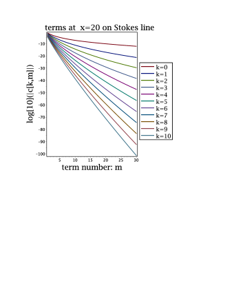
Figure 1. Size of terms in the successive series on the Stokes ray $\mathbb{R}^{+}$ with the formula (69). This plot can be used to determine the number of terms to be kept for a given accuracy. To get $10^{-5}$ accuracy, 10 terms of the first series plus 5 from the second (with $k=1$) and so on, and all terms from the fifth series (with $k=4$) on can be discarded.

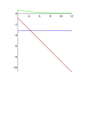
Figure 2. $f(x)=\mathrm{e}^{-x}\mathrm{Ei}^{+}(x)$ on the Stokes line: $\Re f$, (green), $\mathrm{e}^{x}\Im f$, (blue), $\ln(-\Im f)$, (red), from (69). The small exponential is “born” on $\mathbb{R}^{+}$, with half of the residue, as expected by comparing with $\tfrac{1}{2}\mathrm{e}^{-x}\left(\mathrm{Ei}^{+}(x)+\mathrm{Ei}^{-}(x)\right)$.

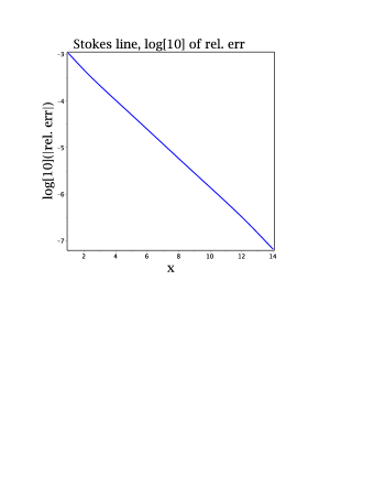
Figure 3. Numerical errors for $x\in[1,14]$ for $\mathrm{e}^{-x}{\rm Ei}^{+}(x)$ along the Stokes line with the formula (69).

Figure 4 below uses the same expansion (69) for $x$ on the two sides of $-i\mathbb{R}^{+}$; in the left picture $\Im\mathrm{e}^{-x}\mathrm{Ei}^{+}(x)$ is calculated for $x\in-i\mathbb{R}-0.3$ and the right one is the graph of $\Im\mathrm{e}^{-x}\mathrm{Ei}^{+}(x)$ along $-i\mathbb{R}+0.3$. The oscillatory behavior is due to the exponential (with amplitude $2\pi i$) collected upon crossing the Stokes ray $\mathbb{R}^{+}$ (arg$\,x=-\pi/2$ is an antistokes ray for Ei⁺).

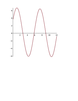
Figure 4. The classical Stokes transition of Ei⁺ from asymptotically decaying to oscillatory.

3.3. Ei away from the Stokes ray, in $\mathbb{C}\setminus\mathbb{R}^{+}$

In §3.1 we used dyadic expansions to obtain geometrically convergent expansions for Ei in $\mathbb{C}\setminus i(-\infty,0]$. In this particular cut plane the convergence is least efficient due to the proximity of the antistokes line where the behavior of Ei is oscillatory. For cut planes that are away by a positive angle from the antistokes line the dyadic expansions are simpler, and more efficient.

Rotating the line of integration in (68) clockwise by an angle $\pi^{-}$ while rotating $x$ anticlockwise by the same angle we obtain its analytic continuation as

(73) $${\rm e}^{-x}{\rm Ei^{+}}(x)=\int_{0}^{\infty e^{-i\pi}}\frac{e^{-px}}{1-p}\,dp=-\int_{0}^{\infty}\frac{e^{px}}{1+p}\,dp\ \ \ \ \ \text{ for }|\arg x-\pi|<\frac{\pi}{2}$$

and we obtain its expression in terms of E₁ (see §9.3):

(74) $${\rm e}^{x}{\rm Ei^{+}}(-x)=-\int_{0}^{\infty}\frac{\mathrm{e}^{-xp}}{p+1}dp=-{\rm e}^{x}{\rm E}_{1}(x)\ \ \ \ \ \text{ for }|\arg x|<\tfrac{\pi}{2}$$

The dyadic expansion of (73) can be obtained as in §3.1. It is convenient to take $\beta=-1$ and change variable to $y=-x$. We obtain:

Proposition 15.

The following identity holds for all $0\neq y\in\mathbb{C}$ with $|\arg\,y|<\pi/2$:

(75) $$\mathrm{e}^{y}{\rm Ei}^{+}(-y)=\sum_{m=1}^{\infty}\frac{(-1)^{m+1}{\mathrm{e}}\Gamma(m)}{(\mathrm{e}-1)^{m}(y)_{m}}-\sum_{k=1}^{\infty}\sum_{m=1}^{\infty}\left({\frac{\Gamma(m)\,{\mathrm{e}^{2^{-k}}}}{\left({\mathrm{e}^{2^{-k}}}+1\right)^{m}{({2}^{k}y)_{m}}}}\right)$$

Of course, in terms of Lech $\Phi$, this is the identity (3).

The remainders are similar to those of Proposition 14.

Note 16.

The effective variable, $2^{k}y$, gets rapidly large for large $k$ and not many terms of the double sum are needed in practice. Even for $y=0.1$ the first sum above (with $k=1$) requires 20 terms to give $10^{-5}$ relative errors.

3.4. Dyadic expansions for the Airy function Ai

The Airy function not only illustrates a non-trivial application of Theorem 6, but also shows how one can handle functions in the Borel plane which have slower decay at $\infty$. We analyze in some detail the Airy function Ai, as the general Bessel functions are dealt with similarly, as explained in §3.5.

After the normalization $f(x)=x^{5/4}\mathrm{e}^{-\frac{2}{3}x^{3/2}}h(4x^{3/2}/3);\ \ x=(3u/4)^{2/3}$, described in more detail in §9.1, the asymptotic series of the Airy function is Borel summable:

(76) $$h(x)=\int_{0}^{\infty}\mathrm{e}^{-px}F(p)dp$$

where $F(p)={{}_{2}F_{1}}(1/6,5/6;1,-p)=P_{-1/6}(1+2p)$ is analytic except for a logarithmic singularity at $-1$, see (117) and (119) below. The decay of $F$ for large $p$ is relatively slow, $O(p^{-1/6})$, see [12](15.8.2), and we integrate once by parts to improve it for Theorem 6 to apply:

(77) $$h(x)=\frac{1}{x}+\frac{1}{x}\int_{0}^{\infty}\mathrm{e}^{-px}F^{\prime}(p)dp$$

where we used ${{}_{2}F_{1}}(1/6,5/6;1,0)=1$. We move the singularity to $1$ by a change of variables after which we can apply Theorem 6 to (78) with $\beta=-1$.

(78) $$h(-x)=-\frac{1}{x}-\frac{1}{x}\int_{0}^{\infty\mathrm{e}^{\pi i}}\mathrm{e}^{-px}F^{\prime}(-p)dp$$

We obtain the dyadic series:

(79) $$h(-x)=-\frac{1}{x}-\sum_{m=1}^{\infty}\frac{\Gamma(m)}{(x)_{m}}d_{m,0}-\sum_{k=1}^{\infty}\sum_{m=1}^{\infty}\frac{\Gamma(m)}{(2^{k}x)_{m}}d_{m,k}$$

Using the branch jump relation (120) we see $\Delta F^{\prime}(-1-t)=-iF^{\prime}(t)$ and hence

(80) $$d_{m,0}=\frac{(-1)^{m+1}}{2\pi}\int_{0}^{\infty}\frac{F^{\prime}(t)\mathrm{e}^{(1+t)}}{(\mathrm{e}^{(1+t)}-1)^{m}}dt;\ \ \ \ \ d_{m,k}=-\frac{1}{2\pi}\int_{0}^{\infty}\frac{F^{\prime}(t){\rm e}^{2^{-k}(1+t)}}{(\mathrm{e}^{2^{-k}(1+t)}+1)^{m}}dt$$

Unlike in the case of Ei, the coefficients $d_{m}$ do not have a simple closed form expression. A convenient, and general, way to determine them numerically is described in §4. There is an interesting expression of these coefficients in the $x$ domain: with $h$ as in (76) and using elementary properties of the Laplace transform we get,

(81) $$\int_{0}^{\infty}\frac{F^{\prime}(t)\mathrm{e}^{t+1}}{(\mathrm{e}^{t+1}-1)^{m}}dt=\sum_{j=0}^{\infty}\mathrm{e}^{-m-j+1}\binom{m+j-1}{j}\int_{0}^{\infty}\mathrm{e}^{-(m+j-1)t}F^{\prime}(t)dt\\ =\mathrm{e}^{1-m}\sum_{j=0}^{\infty}\mathrm{e}^{-j}\binom{m+j-1}{j}[(m+j-1)h(m+j-1)-1]$$

Fig. 5 shows the numerical results from (79) using Mathematica in machine precision to evaluate the integrals in the $d_{m,0},d_{m,k}$.

3.5. General Bessel functions

There are few and relatively minor adaptations needed to deal with $K_{\nu}$ for more general $\nu$. After normalization, explained in §9.1, $F(p)$ is now the Legendre function $P_{\nu-1/2}(1+2p)$ for which the branch jump at $-1$ is $\Delta F(-1-p)=-2i\cos(\pi\nu)F(p)$ (see (119)) and the leading behavior at infinity is $O(p^{|\Re\nu|-1/2})$. The steps followed in the Airy case apply after integrating by parts $k$ times until $|\Re\nu|-1/2-k<-1$. Alternatively, one can apply the general transformation in §20 that ensures exponential decay. For $J_{\nu},Y_{\nu}$ the procedure is the same, except that the singularity is now on the imaginary line. For $J_{\nu}$ the singularity is on $\mathbb{R}^{+}$ and a choice of $\beta$ as for Ei⁺ needs to be made.

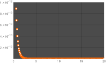
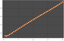
Figure 5. Relative accuracy for Ai (left), and number of exact digits (right) as functions of $x$. The total number of terms used in this calculation ranges from about 150 for small $x$ to 30 terms at $x=20$, found as explained in Fig. 1. The right graph plateaus at 16 digits for all $x\geqslant 4$, an artefact due to calculations being made in Mathematica’s machine precision; thus the right graph was stopped at $x=4$.

4. Practical ways to calculate the dyadic coefficients

For a general function element $F$ the coefficients of its dyadic series are given by the integral formulas (39). However, for any given $F$, these coefficients can be obtained in an efficient way as follows.

The function $F$ is represented with arbitrary accuracy by Padé approximants, which we decompose by partial fractions: $F(p)\approx\sum_{i=1}^{n}\tfrac{c_{i}^{(n)}}{p-p_{i}^{(n)}}$. We assume, as it is typically the case, that the poles are simple. Since $F$ has only one singularity at $p=p_{0}$ (e.g. $p_{0}=1$), the poles $p_{i}^{(n)}$ lie on a half line originating at $p_{0}$ (in our example, on $[1,+\infty)$) [28]. The Padé approximants converge in capacity; however modifications of the approximants converge uniformly at almost the same rate [28]. It then suffices to calculate the dyadic series for each term, $F_{i}^{(n)}(p)=\tfrac{1}{p-p_{i}^{(n)}}$, which reduces to the case of the exponential integral studied in §3.1, whose dyadic coefficients are explicit.

5. Dyadic expansions for the Psi function and a curious identity

The digamma function, or Psi function, defined as

$$\Psi(z)=\frac{\Gamma^{\prime}(z)}{\Gamma(z)}$$

is a meromorphic function with simple poles of residue $-1$ at $z=-1,-2,-3,\ldots$ see [12](5.2.1).

We find, and state in Proposition 17 the dyadic series for the Psi function, and one for differences of Psi functions, which yields a curious identity, (4), which appears to be new.

Proposition 17.

(i) We have, for all $x\in\mathbb{C}\setminus(-\infty,0]$,

(82) $$\Psi(x+1)=\ln x-\sum_{k=1}^{\infty}\Phi(-1,1,2^{k}x+1)=\ln x+\sum_{k=1}^{\infty}\sum_{j=1}^{\infty}{\frac{(j-1)!}{2^{j}(2^{k}x+1)_{j}}}$$

(ii) For all $x\in\mathbb{C}\setminus(-\infty,0]$ we have

(83) $$\frac{1}{2}\Psi\left(\frac{x}{2}+\frac{1}{2}\right)-\frac{1}{2}\Psi\left(\frac{x}{2}\right)=\frac{1}{2x}\ -\ \frac{1}{2^{2}(x)_{2}}+\cdots+\frac{(-1)^{n-1}\Gamma(n)}{2^{n}(x)_{n}}+\cdots$$

For $\Re x>0$ we have

(84) $$\frac{1}{2}\Psi\left(\frac{x}{2}+\frac{1}{2}\right)-\frac{1}{2}\Psi\left(\frac{x}{2}\right)=\int_{0}^{1}\frac{t^{x-1}}{t+1}dt$$

(iii) The identity (4) holds.

Proof.

(i) Replacing $p$ by $-p$ in (18) we get

(85) $$\frac{1}{p}-\frac{1}{\mathrm{e}^{p}-1}=\sum_{k=1}^{\infty}\frac{{\rm e}^{-\frac{p}{{2}^{k}}}}{2^{k}\left({{\rm e}^{-{\frac{p}{{2}^{k}}}}}+1\right)}$$

On the other hand we have, see [10] eq. (4.61) p. 99,

(86) $$\frac{\Gamma^{\prime}(x+1)}{\Gamma(x+1)}-\ln x=\int_{0}^{\infty}\left(\frac{1}{p}-\frac{1}{\mathrm{e}^{p}-1}\right)\mathrm{e}^{-xp}dp$$

Thus, changing the variable of integration to $q=p/2^{k}$ we get

(87) $$\Psi(x+1)=\frac{\Gamma^{\prime}(x+1)}{\Gamma(x+1)}=\ln x+\sum_{k=1}^{\infty}\int_{0}^{\infty}\frac{\mathrm{e}^{-q(1+2^{k}x)}}{1+\mathrm{e}^{-q}}\,dq$$

and integrating by parts we obtain the dyadic factorial expansion (82).

(ii) Consider the functional equation

(88) $$f(x+1)+f(x)=\frac{1}{x}$$

After Borel transform (i.e. substituting (6) in (88)) we obtain $(\mathrm{e}^{-p}+1)F(p)=1$, yielding

(89) $$f(x)=\int_{0}^{\infty}\,\frac{\mathrm{e}^{-px}}{\mathrm{e}^{-p}+1}\,dp=\int_{0}^{\infty}\,\sum_{n=0}^{\infty}\,(-1)^{n}\,\mathrm{e}^{-p(x+n)}\,dp=\sum_{n=0}^{\infty}\frac{(-1)^{n}}{x+n}$$

where the interchange of summation and integration is justified, say, by the monotone convergence theorem applied to $\sum_{n=0}^{2N}(-1)^{n}\mathrm{e}^{-p(x+n)}$. Of course, the integral converges only for $\Re x>0$, but the series converges for all $x\notin\{0,-1,-2,...\}$. Therefore $f(x)$ is meromorphic, having simple poles at $x=-n,\ n\in\mathbb{N}$.

On the other hand $f(x)=\tfrac{1}{2}\psi(\tfrac{x}{2}+\tfrac{1}{2})-\tfrac{1}{2}\psi(\tfrac{x}{2})$ which follows from integrating the identity

$$\psi^{\prime}(z)=\sum_{n=0}^{\infty}(z+n)^{-2}$$

(see [2], (31) p. 200) between $z=\frac{x}{2}$ and $z=\frac{x+1}{2}$.

The integral representation (84) then follows by substituting $\mathrm{e}^{-p}=t$ in (89) and the factorial expansion in (83) is then obtained as usual, by integration by parts.

(iii) is obtained straightforwardly by combining (83) with (82).

∎

6. Duplication formulas and incomplete Gamma functions

Some applications, such as the ones in §6.1 and §7, require fractional powers. In this section Lemma 18 generalizes Lemma 3 to fractional powers of $p$ and find simple dyadic representations for some other classes of special functions. We find factorial series with coefficients having closed form expressions in terms of polylogarithms.

Recall that the polylog is defined as

$$\mathrm{Li}_{s}\left(z\right)=\sum_{k=1}^{\infty}\frac{z^{k}}{k^{s}}$$

for any $s\in\mathbb{C}$. The series converges for $|z|<1$ and $\mathrm{Li}_{s}(z)$ is defined by analytic continuation for other values of $z$, [12]25.12.10. It has the integral representation

(90) $$\mathrm{Li}_{s}\left(z\right)=\frac{z}{\Gamma\left(s\right)}\int_{0}^{\infty}\frac{x^{s-1}}{\mathrm{e}^{x}-z}dx$$

when $\Re s>0$ and $\arg(1-z)<\pi$, or $\Re s>1$ and $z=1$, [12]25.12.11.

$\mathrm{Li}_{s}(z)$ satisfies the general duplication formula

(91) $$f(z)+f(-z)=2^{1-s}f(z^{2})$$

(see [21]; also, (90), (91) are easily checked directly).

Lemma 18 (A ramified generalization of (18)).

The following identity holds in $\mathbb{C}\setminus\{0\}$:

(92) $$\pi p^{s-1}=\Gamma(s)\sin(\pi s)\left[\mathrm{Li}_{s}\left(\mathrm{e}^{-p}\right)-\sum_{k=1}^{\infty}2^{-k(1-s)}\mathrm{Li}_{s}\left(-\mathrm{e}^{-2^{-k}p}\right)\right]\ \ \ \ \text{ if }s<1$$

which reduces to (18) if $s=0$.

Proof.

Let $s<1$. As in the proof of Lemma 3 we iterate (91) $n$ times:

(93) $$f(z)=-f(-z)+2^{1-s}f(z^{2})=-f(-z)-2^{1-s}f(-z^{2})+2^{2(1-s)}f(z^{4})=\ldots\\ =2^{n(1-s)}f\left(z^{2^{n}}\right)-\sum_{j=0}^{n-1}2^{j(1-s)}f\left(-z^{2^{j}}\right)$$

where, taking $z=e^{p/2^{n}}$ we obtain

(94) $$2^{-n(1-s)}\text{Li}_{s}\left(\mathrm{e}^{-p/2^{n}}\right)=\text{Li}_{s}\left(\mathrm{e}^{-z}\right)-\sum_{k=1}^{n}2^{-k(1-s)}\text{Li}_{s}\left(-\mathrm{e}^{-p/2^{k}}\right)$$

We use the following identity [12](25.12.12):

$$\mathop{\mathrm{Li}_{s}\/}\nolimits\!\left(u\right)=\mathop{\Gamma\/}\nolimits\!\left(1-s\right)\left(\mathop{\ln\/}\nolimits\frac{1}{u}\right)^{s-1}+\sum_{j=0}^{\infty}\mathop{\zeta\/}\nolimits\!\left(s-j\right)\frac{(\mathop{\ln\/}\nolimits u)^{j}}{j!},\ \ \ \ \ \ \ \ \ \ \ \ s\neq 1,2,\ldots,\ \ \ \ |\ln u|<2\pi$$

which, for $u=\mathrm{e}^{-p/2^{n}}$ becomes

$$2^{-n(1-s)}\text{Li}_{s}\left(\mathrm{e}^{-p/2^{n}}\right)=\Gamma(1-s)p^{s-1}+2^{-n(1-s)}\sum_{j=0}^{\infty}\mathop{\zeta\/}\nolimits\!\left(s-j\right)\frac{(\mathop{\ln\/}\nolimits u)^{j}}{j!},$$

where we see that, for $s<1$, $\lim_{n\to\infty}2^{-n(1-s)}\text{Li}_{s}\left(\mathrm{e}^{-p/2^{n}}\right)=\Gamma(1-s)p^{s-1}$. Thus, taking the limit $n\to\infty$ in (94) we obtain

$$z^{s-1}\Gamma(1-s)=\text{Li}_{s}\left(\mathrm{e}^{-z}\right)-\sum_{k=1}^{\infty}2^{-k(1-s)}\text{Li}_{s}\left(-\mathrm{e}^{-2^{-k}z}\right)$$

from which (92) follows by using the reflection formula $\Gamma(s)\Gamma(1-s)=\pi/\sin(\pi s)$. ∎

6.1. Dyadic series for incomplete gamma functions and erfc

The incomplete gamma function, which arises as solution to various mathematical problems, is defined by

$$\Gamma(s,x)=\int_{x}^{\infty}\,t^{s-1}\,\mathrm{e}^{-t}\,dt$$

and has as a special case the error function,

$$\text{erfc}(x)=\frac{2}{\sqrt{\pi}}\int_{x}^{\infty}\,\mathrm{e}^{-t^{2}}\,dt=\frac{1}{\sqrt{\pi}}\,\Gamma\left(\frac{1}{2},x^{2}\right)$$

Noting that

$$\int_{0}^{\infty}(1+p)^{s-1}\mathrm{e}^{-xp}dp=\mathrm{e}^{x}x^{-s}\Gamma(s,x)$$

we see that $\mathrm{e}^{x}x^{-s}\Gamma(s,x)$ is the Laplace transform of a function which has a ramified singularity if $s\not\in\mathbb{Z}$. In this case we apply Lemma 18 and obtain the expansion, for $s<1$

(95) $$\Gamma(1-s)\mathrm{e}^{x}x^{-s}\Gamma(s,x)=\mathcal{L}\,\text{Li}_{s}\left(\mathrm{e}^{-p-1}\right)-\sum_{k=1}^{\infty}2^{-k(1-s)}\mathcal{L}\,\text{Li}_{s}\left(-\mathrm{e}^{-2^{-k}(p+1)}\right)$$

and in particular

(96) $$\pi e^{x}x^{-1/2}\text{erfc}\left(\sqrt{x}\right)=\mathcal{L}\,\text{Li}_{\frac{1}{2}}\left(\mathrm{e}^{-p-1}\right)-\sum_{k=1}^{\infty}2^{-k/2}\mathcal{L}\,\text{Li}_{\frac{1}{2}}\left(-\mathrm{e}^{-2^{-k}(p+1)}\right)$$

From this point on, the dyadic expansions are obtained by calculating the factorial expansion of each term in (96). For example, the first term in (96) has the factorial series

(97) $$\mathcal{L}\,\text{Li}_{\frac{1}{2}}\left(\mathrm{e}^{-p-1}\right)=\int_{0}^{1}t^{x-1}\text{Li}_{\frac{1}{2}}\left(\frac{t}{\mathrm{e}}\right)dt=\sum_{k=0}^{\infty}\frac{(-1)^{k}}{\mathrm{e}^{k}(x)_{k+1}}\text{Li}_{\frac{1}{2}}^{(k)}\left(\mathrm{e}^{-1}\right):=\sum_{k=0}^{\infty}\frac{c_{k}}{(x)_{k+1}}$$

with

(98) $$c_{k}=(-1)^{k}\sum_{j=0}^{k}s(k,j)\text{Li}_{\frac{1}{2}-j}\left(\mathrm{e}^{-1}\right)$$

where $s(k,j)$ are the Stirling numbers of the first kind (see §9.2 for details), where we used the formula.

(99) $$\frac{d^{k}}{dz^{k}}\text{Li}_{\nu}\left(z\right)=z^{-k}\sum_{j=0}^{k}s(k,j)\text{Li}_{\nu-j}(z)$$

7. Dyadic resolvent identities

Dyadic decompositions translate into representations of the resolvent of a self-adjoint operator in a series involving the unitary evolution operator at specific discrete times:

Proposition 19.

(i) Let $\mathcal{H}$ be a Hilbert space, and $A$ a bounded or unbounded self-adjoint operator. Let $U$ be the unitary evolution operator generated by $A$, $U_{t}=\mathrm{e}^{-itA}$. If $\lambda\in\mathbb{R}^{+}$, then

(100) $$(A-i\lambda)^{-1}=i(1-\mathrm{e}^{-\lambda}U_{1})^{-1}-i\sum_{k=1}^{\infty}\frac{1}{2^{k}}(1+e^{-{\lambda}/2^{k}}U_{2^{-k}})^{-1}$$

and (5) follows.

Convergence holds in the strong operator topology. For $\lambda<0$ one simply complex conjugates (100). (The limits cannot, generally, be interchanged.)

(ii) Assume $A$ is a positive operator (thus self-adjoint) and $0\notin\sigma(A)$. Let $T_{t}$ be the semigroup generated by $A$, $T_{t}=\mathrm{e}^{-tA}$. Then

(101) $$A^{-1}=(1-T_{1})^{-1}-\sum_{k=1}^{\infty}2^{-k}(1+T_{1/2^{k}})^{-1}=\sum_{j=1}^{\infty}T_{j}-\lim_{\ell\to\infty}\sum_{k=1}^{\ell}\sum_{j=1}^{\infty}2^{-k}(-1)^{j}T_{j/2^{k}}$$

where now convergence is in operator norm. More generally, for $s<1$, $s\notin\mathbb{Z}$,

(102) $$\pi A^{s-1}=\Gamma(s)\sin(\pi s)\left[\mathrm{Li}_{s}\left(T_{1}\right)-\sum_{k=1}^{\infty}2^{-k(1-s)}\mathrm{Li}_{s}\left(-T_{1/2^{k}}\right)\right]$$

in operator norm

For a discussion of the polylog function $\mathrm{Li}_{s}(z)$ see §6.

Proof.

(i) We recall the projection-valued measure spectral theorem for self-adjoint operators. If $\mathcal{H}$ and $A$ are as above and $g:\mathbb{R}\to\mathbb{R}$ is a Borel function (or a complex one, by writing $g=g_{1}+ig_{2}$), then $g(A)=\int_{-\infty}^{\infty}g(q)dP_{q}$ where $\{P_{\Omega}\}$ are the projection-valued measures induced by $A$ on $\sigma(A)$ (see [25] Theorem VIII.6 p. 263). The spectral theorem together with (26) for $p=\lambda+iq$ give

(103) $$(1-\mathrm{e}^{-\lambda}U_{1})^{-1}-\sum_{k=1}^{n}2^{-k}(1+\mathrm{e}^{-2^{-k}\lambda}U_{2^{-k}})^{-1}=\varepsilon(1-\mathrm{e}^{-\lambda\varepsilon}\mathrm{e}^{-i\varepsilon A})^{-1}=\int_{\mathbb{R}}\frac{\varepsilon dP_{q}}{1-\mathrm{e}^{-\varepsilon(\lambda+iq)}}$$

where $\varepsilon_{n}:=\varepsilon=2^{-n}$. An elementary calculation shows that the modulus of the integrand is uniformly bounded by $\lambda^{-1}$. Since the integrand converges pointwise to $(\lambda+iq)^{-1}$ as $\varepsilon\to 0$, dominated convergence shows that the integral converges to $(\lambda+iA)^{-1}$. Dominated convergence also shows that the integrand, seen as a multiplication operator, converges in the strong operator topology, implying the result.

(ii) The proof, based on the same argument as in (i), is simpler and we omit it. For (102) we combine this argument with Lemma 18 below. The sums in (101) are manifestly convergent in the operator norm since $\|T_{t}\|<1$ and $T_{t}>0$. ∎

8. Dyadic series of typical functions occurring in applications; resurgence

Generic systems of meromorphic ODEs, difference equations and other classes of problems commonly occurring in applications have solutions characterized by a special Borel plane structure:

1. they have at most exponential growth at infinity (meaning a finite exponentially weighted $L^{1}$ norm; see §8.2)

2. their singularities are equally spaced along finitely many rays and

3. at each singularity there exists locally Frobenius-type convergent expansions in fractional powers and possibly logs (see e.g. [9, 8]).

Let us say that functions having properties (1)-(3) satisfy assumption (A). In fact, more is true for the aforementioned solutions: the singularities on the Riemann surface of solutions of the same equation are interconnected in an explicit fashion, and possess a set of deep properties –they are resurgent in the sense of Écalle, see [15, 9].

8.1. Decomposition of resurgent functions into function elements

We defined function elements to be resurgent functions with only one regular singularity on the first Riemann sheet, and with algebraic decay at infinity, see §2.2.1. There are two main properties of function elements which do not hold for general resurgent functions: decay at infinity in $p$ and the property of having only one singularity. However, resurgent functions can be decomposed into elements:

Theorem 20.

The Laplace transform of functions satisfying assumption (A) can be written, modulo a convergent series at infinity and translations of the variable, as a sum of Laplace transforms of resurgent elements plus an entire function.

Note 21.

The exponential integral and the $\Psi$ function treated in §5 are examples of elements with nonramified singularities. Airy and Bessel functions treated in §3.4 and §3.5 are examples of elements with ramified singularities, treated via the Cauchy kernel decomposition. The incomplete gamma function and the error function treated in §6.1 have power-ramified singularities for which a polylog dyadic expansion (Lemma 18) gives more explicit decompositions. Theorem 20 extends these techniques to general resurgent functions.

8.2. Decomposition in resurgent elements

In this section we describe how a general resurgent function can be decomposed into resurgent elements. To avoid cumbersome details and keep the presentation clear, we present the essential steps in the case where the resurgent function has the form encountered in generic meromorphic ODEs.

Denoting the singularities of the resurgent function $F$ by $\omega_{i}$, we thus assume:

1. Each $\omega_{i}$ is of the form $j\lambda_{k}$, with $j\in\mathbb{Z}^{+}$ and $\lambda_{k}\in\{\lambda_{1},\ldots,\lambda_{n}\}$ (the eigenvalues of the linearization of the ODE at $\infty$, which are assumed to be linearly independent over $\mathbb{Z}$ and of different complex arguments);

2. there is a $\nu>0$ such that the following sup is bounded:

   $$\|F\|_{1,\nu}:=\sup_{\varphi\in[0,2\pi]}\int_{0}^{\infty\mathrm{e}^{i\varphi}}|F(p)|\mathrm{e}^{-\nu|p|}d|p|<\infty$$

   We denote by $S_{i}$ thin, non-intersecting half-strips containing exactly one singularity $\omega_{i}$; let $\mathcal{A}$ be the complement of the union of $S_{i}$. We let $\mathcal{C}_{i}=\partial S_{i}$, see Fig. 6. $\mathcal{C}_{i}$ are non-intersecting Hänkel contours around the $\omega_{i}$, going vertically if $\omega_{i}$ belongs to a singularity ray in the open right half plane and towards $\infty$ in the left half plane otherwise; $\mathcal{C}_{i}$ are traversed anticlockwise.

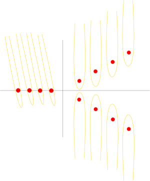
Figure 6. The yellows contours are the $\mathcal{C}_{i}$, plotted almost vertical for clarity.

Let

(104) $$G(p)=F(p)-\sum_{\omega_{i}}\frac{\exp(\mu_{i}p)}{2\pi i}\int\limits_{\mathcal{C}_{i}}\frac{F(s)\exp(-\mu_{i}s)}{s-p}ds$$

where:

1. $|\mu_{i}|=\mu>\nu$,

2. $\arg(\mu_{i})$ is the negative of the angle of the contour $\mathcal{C}_{i}$, i.e., in each integral in (104), $\mu_{i}s\in\mathbb{R}^{+}$ for large $s$. Note that the set $\{\arg\mu_{i}\}$ is finite, since there are only finitely many rays with singularities.

8.3. Proof of Theorem 20

Proof.

We show that the function defined by (104) is entire and satisfies necessary growth conditions for Theorem 20 to hold.

We analyse each summand in (104) individually denoting them as $F_{i}$: let

(105) $$F_{i}(p)=\frac{\exp(\mu_{i}p)}{2\pi i}\int\limits_{\mathcal{C}_{i}}\frac{F(s)\exp(-\mu_{i}s)}{s-p}ds$$

Lemma 22.

There exists $\nu^{\prime}>0$ such that for each singular point $\omega_{i}$, the corresponding $F_{i}$ belongs to $L^{1}_{\nu^{\prime}}$.

Proof.

Let $\omega_{i}$ be a singular point of $F$ and without loss of generality assume $\omega_{i}\in\mathbb{R}^{+}$ (this can be achieved for each $i$ by an appropriate rotation of the complex plane). The exponential weight $\nu^{\prime}>\nu$ will be chosen later based upon additional conditions. For a given $\varepsilon>0$, we estimate the norm of $F_{i}$ in $L^{1}_{\nu^{\prime}}(\mathrm{e}^{i\varphi}\mathbb{R}^{+})$ in two cases of the direction $\varphi$.

$$A=(\varepsilon,2\pi-\varepsilon),\quad B=[-\varepsilon,\varepsilon]$$

Let first $\varphi\in A$. We deform the contour $\mathcal{C}_{i}$ into sector $B$ so that it forms an angle $\varepsilon/2$ with $\mathbb{R}^{+}$. We have

$$\int_{\mathrm{e}^{i\varphi}\mathbb{R}^{+}}\mathrm{e}^{-\nu^{\prime}|p|}|F_{i}(p)|d|p|\leq\int_{\mathrm{e}^{i\varphi}\mathbb{R}^{+}}\mathrm{e}^{-\nu^{\prime}|p|}\frac{|\mathrm{e}^{\mu_{i}p}|}{2\pi}\int_{\omega_{i}+\mathrm{e}^{\frac{i\varepsilon}{2}}[0,\infty)}\frac{|\Delta F(s)\mathrm{e}^{-\mu_{i}s}|}{|s-p|}d|s|d|p|$$

Using the estimate $|s-p|\geq\omega_{i}\sin\varepsilon$ for all $s\in\mathcal{C}_{i}$ and $p\in\mathrm{e}^{i\varphi}\mathbb{R}^{+}$ we get

$$\|F_{i}\|_{L_{\nu^{\prime}}^{1}(\mathrm{e}^{i\varphi}\mathbb{R}^{+})}\leq\frac{|\mathrm{e}^{-\mu_{i}\omega_{i}}|}{\pi\omega_{i}\sin\varepsilon[\nu^{\prime}-|\mu_{i}|\cos(\arg\mu_{i}+\varphi)]}\|F\|_{1,\nu}$$

Let now $\varphi\in B$. We first deform the contour to avoid any crossing of $\mathcal{C}_{i}$ and $\mathrm{e}^{i\varphi}\mathbb{R}^{+}$. To this end we represent $F_{i}$ as

$$F_{i}(p)=F_{i}(p)\mathcal{H}\big{(}\frac{\omega_{i}}{2}-|p|\big{)}+F_{i}(p)\Big{[}\mathcal{H}\big{(}|p|-\frac{\omega_{i}}{2}\big{)}-\mathcal{H}\big{(}|p|-\frac{3\omega_{i}}{2}\big{)}\Big{]}+F_{i}(p)\mathcal{H}\big{(}|p|-\frac{3\omega_{i}}{2}\big{)}$$

$\mathcal{H}$ is the Heaviside function with the convention $\mathcal{H}(x)=\mathbbm{1}_{(0,\infty)}(x)+\frac{1}{2}\mathbbm{1}_{\{0\}}(x)$. We have

(106) $$\|F_{i}\|_{1,\nu^{\prime}}\leq\int_{\mathrm{e}^{i\varphi}[0,\frac{\omega_{i}}{2}]}\mathrm{e}^{-\nu^{\prime}|p|}|F_{i}(p)|d|p|+\int_{\mathrm{e}^{i\varphi}[\frac{\omega_{i}}{2},\frac{3\omega_{i}}{2}]}\mathrm{e}^{-\nu^{\prime}|p|}|F_{i}(p)|d|p|+\int_{\mathrm{e}^{i\varphi}[\frac{3\omega_{i}}{2},\infty)}\mathrm{e}^{-\nu^{\prime}|p|}|F_{i}(p)|d|p|$$

The first term $F_{i}$ is actually bounded in a weighted $\sup$-norm since $|s-p|\geq|\omega_{i}|/2$ for all $s\in\mathcal{C}_{i}$

$$|F_{i}(p)|\leq\frac{|\mathrm{e}^{\mu_{i}p}|}{\pi\omega_{i}}\int_{\omega_{i}+\mathrm{e}^{\frac{i\varepsilon}{2}}[0,\infty)}|\Delta F(s)\mathrm{e}^{-\mu_{i}s}|d|s|\leq\frac{2|\mathrm{e}^{\mu_{i}p}\mathrm{e}^{-(\mu_{i}-\nu)\omega_{i}}|}{\pi\omega_{i}}\|F\|_{1,\nu}$$

which implies

(107) $$\int_{\mathrm{e}^{i\varphi}[0,\frac{\omega_{i}}{2}]}\mathrm{e}^{-\nu^{\prime}|p|}|F_{i}(p)|d|p|\leq\frac{2|\mathrm{e}^{-(\mu_{i}-\nu)\omega_{i}}|}{\pi\omega_{i}}\|F\|_{1,\nu}\int_{0}^{\infty\mathrm{e}^{i\varphi}}\mathrm{e}^{-\nu^{\prime}|p|}|\mathrm{e}^{\mu_{i}p}|d|p|\\ =\frac{2|\mathrm{e}^{-(\mu_{i}-\nu)\omega_{i}}|}{\pi\omega_{i}[\nu^{\prime}-|\mu_{i}|\cos(\arg\mu_{i}+\varphi)]}\|F\|_{1,\nu}$$

We estimate the third integral in a similar way to the first using $\{\omega_{i}+t\mathrm{e}^{\frac{3\varepsilon}{2}i}:t\geq 0\}$ as the contour of integration for the definition of $F_{i}$. Under these conditions we have $|s-p|\geq\omega_{i}(\frac{3}{2}\sin\frac{\varepsilon}{2}-\sin\frac{3\varepsilon}{2})$

(108) $$\int_{\mathrm{e}^{i\varphi}[\frac{3\omega_{i}}{2},\infty)}\mathrm{e}^{-\nu^{\prime}|p|}|F_{i}(p)|d|p|\\ \leq\frac{1}{2\pi\omega_{i}(\frac{3}{2}\sin\frac{\varepsilon}{2}-\sin\frac{3\varepsilon}{2})}\int_{\mathrm{e}^{i\varphi}[\frac{3\omega_{i}}{2},\infty)}\mathrm{e}^{-\nu^{\prime}|p|}|\mathrm{e}^{\mu_{i}p}|\int_{\omega_{i}+\mathrm{e}^{\frac{3\varepsilon}{2}i}[0,\infty)}|\Delta F(s)\mathrm{e}^{-\mu_{i}s}|d|s|d|p|\\ \leq\frac{\|F\|_{1,\nu}|\mathrm{e}^{-(\mu_{i}-\nu)\omega_{i}}|}{\pi\omega_{i}(\frac{3}{2}\sin\frac{\varepsilon}{2}-\sin\frac{3\varepsilon}{2})}\int_{\mathrm{e}^{i\varphi}[\frac{3\omega_{i}}{2},\infty)}\mathrm{e}^{-\nu^{\prime}|p|}|\mathrm{e}^{\mu_{i}p}|d|p|\\ \leq\frac{\|F\|_{1,\nu}|\mathrm{e}^{-(\mu_{i}-\nu)\omega_{i}}|}{\pi\omega_{i}(\frac{3}{2}\sin\frac{\varepsilon}{2}-\sin\frac{3\varepsilon}{2})[\nu^{\prime}-|\mu_{i}|\cos(\arg\mu_{i}+\varphi)]}\mathrm{e}^{-\frac{3\omega_{i}}{2}[\nu^{\prime}-|\mu_{i}|\cos(\arg\mu_{i}+\varphi)]}$$

We estimate the second term of 106 by deforming $\{\omega_{i}+\mathrm{e}^{i\varepsilon/2}\mathbb{R}^{+}\}$ into another contour denoted by $\tilde{\mathcal{C}}_{i}$. The deformation is such that it subsumes the line segment $\mathrm{e}^{i\varphi}[\frac{\omega_{i}}{2},\frac{3\omega_{i}}{2}]$ so its leftmost point of intersection with $\mathbb{R}^{+}$ occurs at $\omega_{i}/4$, and remains in region $B$ such that the minimal distance of $\tilde{\mathcal{C}}_{i}$ to the segment $\mathrm{e}^{i\varphi}[\frac{\omega_{i}}{2},\frac{3\omega_{i}}{2}]$ is $\frac{\omega_{i}}{4}\sin\varepsilon/2$. The contour deformation will collect a residue at each $p$ and results in

(109) $$\int_{\mathrm{e}^{i\varphi}[\frac{\omega_{i}}{2},\frac{3\omega_{i}}{2}]}\mathrm{e}^{-\nu^{\prime}|p|}|F_{i}(p)|d|p|\\ =\int_{\mathrm{e}^{i\varphi}[\frac{\omega_{i}}{2},\frac{3\omega_{i}}{2}]}\mathrm{e}^{-\nu^{\prime}|p|}\Bigg{|}\frac{\exp(\mu_{i}p)}{2\pi i}\left[\int\limits_{\tilde{\mathcal{C}}_{i}}\frac{F(s)\exp(-\mu_{i}s)}{s-p}ds+2\pi iF(p)\exp(-\mu_{i}p)\right]\Bigg{|}d|p|\\ \leq\frac{4\|F\|_{1,\nu}}{\pi\omega_{i}}\int_{\mathrm{e}^{i\varphi}[\frac{\omega_{i}}{2},\frac{3\omega_{i}}{2}]}\mathrm{e}^{-\nu^{\prime}|p|}|\mathrm{e}^{\mu_{i}p}|d|p|+\int_{\mathrm{e}^{i\varphi}[\frac{\omega_{i}}{2},\frac{3\omega_{i}}{2}]}\mathrm{e}^{-\nu^{\prime}|p|}|F(p)|d|p|\\ =\frac{4\|F\|_{1,\nu}\mathrm{e}^{-\frac{\omega_{i}}{2}[\nu^{\prime}-|\mu_{i}|\cos(\arg\mu_{i}+\varphi)]}}{\pi\omega_{i}[\nu^{\prime}-|\mu_{i}|\cos(\arg\mu_{i}+\varphi)]}+\mathrm{e}^{-\nu^{\prime}|\omega_{i}|/2}\|F\|_{1,\nu^{\prime}}$$

Therefore for any $\nu^{\prime}>\nu$ we have $\|F_{i}\|_{1,\nu^{\prime}}<\infty$. The estimate for $\Re\omega_{i}<0$ is similar the only difference being the orientation of the branch cuts and Hänkel contours. ∎

Lemma 23.

In any compact set in $\mathcal{A}$, the sum in (104) converges at least as fast as $\sum_{j\in\mathbb{Z}^{+},k=1,...,n}\mathrm{e}^{-j|\lambda_{k}|(\mu-\nu)}$ in the $L^{1}_{\nu^{\prime}}$ norm.

Proof.

This follows from an application of the $L^{1}_{\nu^{\prime}}$ estimates obtained in 22 and recalling $\omega_{i}=j\lambda_{k}$ for $j\in\mathbb{N}$ and $\lambda_{k}$ the eigenvalues of a linearized ODE. ∎

Lemma 24.

On the first Riemann sheet, each $F_{i}$ in (105) has precisely one singularity, namely at $\omega_{i}$. Furthermore $F-F_{i}$ is analytic at $\omega_{i}$.

Proof.

Let $p\neq\omega_{i}$. If $p$ is outside $\mathcal{C}_{i}$ then function $F_{i}$ is manifestly analytic at $p$. To analytically continue in $p$ to the interior of $\mathcal{C}_{i}$ it is convenient to first deform $\mathcal{C}_{i}$ past $p$, collecting the residue. We get

(110) $$F_{i}(p)=\frac{\exp(\mu_{i}p)}{2\pi i}\left[\int\limits_{\tilde{\mathcal{C}}_{i}}\frac{F(s)\exp(-\mu_{i}s)}{s-p}ds+2\pi iF(p)\exp(-\mu_{i}p)\right]\\ =F(p)+\frac{\exp(\mu_{i}p)}{2\pi i}\int\limits_{\tilde{\mathcal{C}}_{i}}\frac{F(s)\exp(-\mu_{i}s)}{s-p}ds$$

where now $p$ sits inside $\tilde{\mathcal{C}}_{i}$, and the new integral is again manifestly analytic.

Thus $F_{i}$ is singular only at $p=\omega_{i}$, and $F-F_{i}$ is analytic at $\omega_{i}$. ∎

Lemma 25.

The function

(111) $$G(p)=F(p)-\sum_{i}F_{i}$$

is entire and $G(p)\mathrm{e}^{-\mu^{\prime}|p|}\in L^{\infty}(\mathrm{e}^{i\varphi}\mathbb{R}^{+})$ for any $\mu^{\prime}\geq\nu^{\prime}$ and any $\varphi\in[0,2\pi]$.

Proof.

Analyticity follows from the monodromy theorem, since $G$ has analytic continuation along any ray in $\mathbb{C}$. To see the bound we consider the antiderivative of $G$. Let $H(p)=\int_{0}^{p}G(s)ds$ and estimate

$$|H(p)|\leq\mathrm{e}^{\nu^{\prime}|p|}\Big{|}\int_{0}^{p}\mathrm{e}^{-\nu^{\prime}|s|}G(s)ds\Big{|}\leq\mathrm{e}^{\nu^{\prime}|p|}\|G\|_{1,\nu^{\prime}}$$

hence $H$ is exponentially bounded of order one. Let $R>0$, using Cauchy’s theorem and $G(p)=H^{\prime}(p)$ we have

$$|G(p)|\leq\frac{1}{2\pi}\oint_{|s|=R}\frac{|H(s)|}{|s-p|^{2}}d|s|\leq\frac{1}{2\pi}\int_{0}^{2\pi}\frac{\mathrm{e}^{\nu^{\prime}|p|}\|G\|_{1,\nu^{\prime}}}{(R-|p|)^{2}}Rdt=\frac{R\mathrm{e}^{\nu^{\prime}|p|}\|G\|_{1,\nu^{\prime}}}{(R-|p|)^{2}}$$

for any $|p|<R$. Letting $R\to\infty$ implies the uniform exponential bound.

∎

Lemma 26.

$g=\mathcal{L}G$ has a convergent asymptotic series at infinity, and is equal to the sum of the series.

Proof.

Expanding $G$ into a power series about the origin $G(p)=\sum_{n=0}^{\infty}a_{n}p^{n}$ with $a_{n}=\frac{G^{(n)}(0)}{n!}$ which is also an asymptotic series. Watson’s lemma shows

$$g=\mathcal{L}G\sim\sum_{n=0}^{\infty}\frac{n!a_{n}}{x^{n+1}}=\sum_{n=0}^{\infty}\frac{G^{(n)}(0)}{x^{n+1}}$$

as $x\to\infty$ along any direction in $\mathbb{C}$.
Moreover, the uniform bound we have for $G$ and Cauchy estimates provide $|G^{(n)}(0)|\lesssim\mu^{\prime n}$ where $\mu^{\prime}$ is as in (111). Therefore, if $|x|$ is large enough the expansion for $g$ at infinity will converge. The function $h(z)=g(1/z)$ is bounded at zero and single-valued, as is seen by deformation of contour (since $G$ is exponentially bounded and entire). Thus $h$ is analytic at zero, and therefore the sum of its asymptotic (=Taylor) series at zero. ∎

Lemma 27.

Each function $\mathrm{e}^{-\mu_{i}p}F_{i}$ decays like $1/p$ as $p\to\infty$.

Proof.

As in 24, by contour deformation we may assume $p$ lies within the contour of integration defining $F_{i}$. Otherwise, by 24 we know know the only singularity of of $F_{i}$ to be $\omega_{i}$ which lies within the contour and by assumption, $F_{i}$ is exponentially bounded at infinity. Using $\eqref{eq:ResidueResurg}$ we see

$$p\mathrm{e}^{-\mu_{i}p}F_{i}(p)=p\mathrm{e}^{-\mu_{i}p}F(p)+\frac{1}{2\pi i}\int\limits_{\tilde{\mathcal{C}}_{i}}\frac{pF(s)\exp(-\mu_{i}s)}{s-p}ds$$

The first term is decaying exponentially. In the second term, we notice that the integrand converges pointwise to the function $-F(s)\mathrm{exp}(-\mu_{i}s)$ as $p\to\infty$. Moreover, by assumption $\mu_{i}s>0$ for large $s$ and $\mu_{i}>\nu$ which imply

$$|F(s)\mathrm{exp}(-\mu_{i}s)|\leq\|F\|_{\nu}|\mathrm{exp}(-s(\mu_{i}-\nu))|$$

which is $L^{1}$. Using the dominated convergence theorem and the singlevaluedness of the exponential function implies the result. ∎

Lemma 28.

The change of variable $\tilde{x}=x-\mu_{i}$ leads to $\mathcal{L}[F_{i}](x)=\mathcal{L}[\tilde{F}_{i}](\tilde{x})$ where $\tilde{F}_{i}$ decays like $1/p$ as $p\to\infty$.

Combining these lemmas, Theorem 20 follows.

∎

9. Appendix

9.1. Normalized Airy and Bessel functions

The modified Bessel equation is

(112) $$x^{2}y^{\prime\prime}+xy^{\prime}-(\nu^{2}+x^{2})y=0$$

The transformation $y=\mathrm{e}^{-x}x^{1/2}h(2x)$, $u=2x$ brings (112) to the normalized form

(113) $$h^{\prime\prime}-\left(1-\frac{2}{u}\right)h^{\prime}-\left(\frac{1}{u}-\frac{1}{4u^{2}}+\frac{\nu^{2}}{u^{2}}\right)h=0$$

This normalized form is suitable for Borel summation since it admits a formal power series solution in powers of $u^{-1}$ starting with $u^{-1}$; it is further normalized to ensure that the Borel plane singularity is placed at $p=-1$. One way to obtain the transformation is to rely on the classical asymptotic behavior of Bessel functions and seek a transformation that formally leads to a solution as above.

The Airy equation

(114) $$f^{\prime\prime}-xf=0$$

can be brought to the Bessel equation with $\nu=1/3$. The normalizing transformation can be obtained from (113), or directly, based on the asymptotic behavior at $\infty$ which suggests the change of variables

$$f(x)=x^{5/4}\mathrm{e}^{-\frac{2}{3}x^{3/2}}h(4x^{3/2}/3);\ \ \ \ \ \ x=(3u/4)^{2/3}$$

bringing the equation to

(115) $$h^{\prime\prime}-\left(1-\frac{2}{u}\right)h^{\prime}-\left(\frac{1}{u}-\frac{5}{36u^{2}}\right)h=0$$

which is indeed (113) for $\nu=1/3$. From this point, without notable algebraic complications we analyze (113).

The inverse Laplace transform of (113) is

(116) $$p(p+1)H^{\prime\prime}(p)+(2p+1)H^{\prime}(p)+\left(\frac{1}{4}-\nu^{2}\right)H(p)=0$$

which is a hypergeometric equation [12]15.10. Its solution which is analytic at $p=0$ is (a constant multiple of)

(117) $$\ _{2}F_{1}\left(\tfrac{1}{2}+\nu,\tfrac{1}{2}-\nu;1;-p\right)=P_{\nu-\frac{1}{2}}(1+2p)$$

where $\,{}_{2}F_{1}$ is the usual hypergeometric function [12](14.3.1) and $P_{\mu}$ is the Legendre $P$ function. On the first Riemann sheet, the solution has two regular singularities, $p=-1$ and $p=\infty$. The behavior at zero is [12](15.2.1)

$$P_{\nu-\frac{1}{2}}(1+2p)=1+\left(\nu^{2}-\frac{1}{4}\right)p+\frac{1}{64}\left(16\nu^{4}-40\nu^{2}+9\right)p^{2}+\cdots$$

At $p=-1$ (with the phase of the log being the usual one for $p+1>0$ we have

(118) $$P_{\nu-\frac{1}{2}}(1+2p)=c_{1}\,\log(p+1)+c_{2}+c_{3}(p+1)\log(p+1)+c_{4}(p+1)+\ldots$$

where $c_{j}=c_{j}(\nu)$ are nonzero constants.

Using properties of the hypergeometric function [12](15.2.3) ${}_{2}F_{1}(a,b;c;z)$ and its relation (117) to the Legendre $P$ function, we recover the branch jump across the cut $(-\infty,-1]$

(119) $$P_{\nu-\frac{1}{2}}^{+}(1+2p)-P_{\nu-\frac{1}{2}}^{-}(1+2p)=\frac{2\pi i}{\Gamma\big{(}\frac{1}{2}+\nu\big{)}\Gamma\big{(}\frac{1}{2}-\nu\big{)}}P_{\nu-\frac{1}{2}}(-1-2p)=2i\cos(\pi\nu)P_{\nu-\frac{1}{2}}(-1-2p)$$

Where we used the reflection formula for the Gamma function to obtain the last equality. We differentiate (119) to obtain the branch jump for the derivative which will be used in §3.4.

(120) $$\Delta P_{\nu-\frac{1}{2}}^{\prime}(1+2p)=-2i\cos(\pi\nu)P_{\nu-\frac{1}{2}}^{\prime}(-1-2p)$$

We note that such a simple relation for the branch jump stems from the fact that the Airy function satisfies a linear second order ODE and does not hold in general.

9.2. The derivatives of the polylogarithm

Here we show that the coefficients $s(k,j)$ which appear in (98) are the Stirling numbers of the first kind.

For $k=0$ we have $s(0,0)=1$. It is easy to check that Li${}_{s}^{\prime}(z)=z^{-1}$Li${}_{s-1}(z)$ confirming that $s(1,0)=0$ and $s(1,1)=1$. For higher $k$ formula (99) is then checked by a simple induction, which leads to the recurrence relations

$$s(k+1,0)=-ks(k,0),\ \ s(k+1,k+1)=s(k,k),\ \ s(k+1,j)=-ks(k,j)+s(k,j-1)$$

which are the recurrence relations satisfied by the Stirling numbers of the first kind, see [12] Sec.26.8.

We note that the polylog is another example when the factorial series converges geometrically in a cut plane.

9.3. More about Ei

We note that $E_{1}$ can be written in a form that allows for analytic continuation through the cut on $\mathbb{R}_{-}$: by elementary changes of variables we have, for $z>0$,

$$E_{1}(z):=\int_{z}^{\infty}\frac{e^{-t}}{t}\,dt=e^{-z}\int_{0}^{\infty}\frac{e^{-pz}}{1+p}\,dp$$

It is interesting to note the relation [12] 6.2.4

$$E_{1}(z)={\rm Ein}(z)-\ln z-\gamma,\ \ \ \ \ \ \text{where }\ \ \ {\rm Ein}(z)=\int_{0}^{z}\frac{1-e^{-t}}{t}\,dt$$

Since Ein is an entire function, and ln is defined with the usual branch for $z>0$, we see that upon analytic continuation across $\mathbb{R}_{-}$, the function $E_{1}$ gains a $2\pi i$; thus $\mathbb{R}_{-}$ is a Stokes line.

For us it is convenient to place this Stokes line along $\mathbb{R}_{+}$, so we work with $-E_{1}(-z)$:

$$-E_{1}(-z)=-e^{z}\int_{0}^{\infty}\frac{e^{pz}}{1+p}\,dp,\ \ (z<0)$$

which analytically continued to the first quadrant yields our Ei⁺ defined in (68).

Note the structure of the branch point at $0$:

$${\rm Ei}^{+}(z)=-{\rm Ein}(-z)+\ln(-z)+\gamma$$

where $\ln(-z)$ has the usual brach for $z<0$ and then it is analytically continued on the Riemann surface of the log (and ${\rm Ein}(-z)$ is entire).

For $e^{-x}$Ei${}^{+}(x)$, $\mathbb{R}^{+}$ is a Stokes ray and the two sides of $i\mathbb{R}^{-}$ are antistokes lines. The behavior of $e^{-x}$Ei${}^{+}(x)$ is oscillatory when $\arg(x)=-\pi/2$ and it is given by an asymptotic series when $\arg(x)=3\pi/2$.

9.4. Proof of Lemma 10

The function $\Phi(z,1,x)$ is defined as (see [12] 25.14.1)

$$\Phi(z,1,x)=\sum_{n=0}^{\infty}\frac{z^{n}}{x+n},\ \ \ \ \ \text{for }x\in\mathbb{C}\setminus\mathbb{Z}_{-},\ |z|<1$$

and for other values of $z$, it is defined by analytic continuation.

Clearly $\Phi(z,1,x)$ is a meromorphic function of $x$ (for $|z|<1$).

For $\Re x>0$ and $|z|<1$, $\Phi$ has the integral representation

(121) $$\Phi(z,1,x)=\int_{0}^{\infty}\frac{e^{-xp}}{1-ze^{-p}}dp$$

(see [12] 25.14.5). Note that the right hand side of (121) is analytic in $z$ in $\mathbb{C}\setminus[1,\infty)$, hence (121) holds in this domain.

Then, for $\Re x>0$ and $|z|<1$, by dominated convergence and using (13), we get

(122) $$\Phi\left(\frac{z}{z-1},1,x\right)=(1-z)\int_{0}^{\infty}\frac{e^{-xp}}{1-z(1-e^{-p})}dp=(1-z)\int_{0}^{\infty}e^{-xp}\sum_{k\geqslant 0}z^{k}(1-e^{-p})^{k}dp\\ =(1-z)\sum_{k\geqslant 0}z^{k}\mathcal{L}(1-e^{-p})^{k}=(1-z)\sum_{k\geqslant 0}z^{k}\frac{k!}{(x)_{k+1}}:=(1-z)\mathcal{E}(x,z)$$

We now show that the series $\mathcal{E}(x,z)$ converges uniformly for $x$ in any compact set disjoint from $\mathbb{Z}_{-}$. Once this is proved it follows that the equality

(123) $$\Phi\left(\frac{z}{z-1},1,x\right)=(1-z)\sum_{k\geqslant 0}z^{k}\frac{k!}{(x)_{k+1}}$$

holds for all $x\in\mathbb{C}\setminus\mathbb{Z}_{-},\ |z|<1$.

We fix $z$ with $|z|<1$. Let $K$ be a compact set disjoint from $\mathbb{Z}_{-}$. Let $\lambda$ be such that $|z|\leqslant\lambda<1$. Let $M$ be as assumed in (49).

We prove that $S_{n}=\sum_{k=M}^{n}z^{k}\frac{k!}{(x)_{k+1}}$ converges uniformly in the following steps outlined below.

(i) Clearly $S_{n}$ satisfies the recurrence

(124) $$f_{n}-f_{n-1}=z^{n}\frac{n!}{(x)_{n+1}}$$

(ii) We show that the recurrence (124) has a unique solution of the form

(125) $$f_{n}=z^{n}\frac{n!}{(x)_{n+1}}\left(\frac{z}{z-1}+\frac{u_{n}}{1-z}\right)$$

where $u_{n}\to 0$. (iii) We then show that $f_{n}\to 0$. (iv) Since the general solution of the recurrence (124) is $f_{n}+C$, it follows that $\sum_{k=M}^{n}z^{k}\frac{k!}{(x)_{k+1}}=f_{n}+C$ for some $C$, hence the series $\sum_{k=M}^{\infty}z^{k}\frac{k!}{(x)_{k+1}}$ converges. (v) Finally, we estimate the remainder of this series.

Proof of (ii)-(iv).

(ii) Assume $\{f_{n}\}_{n}$ satisfies (124). Let $u_{n}$ be given by (125). Then $u_{n}$ satisfies

(126) $$u_{n-1}=\frac{xz}{(x+n)}+\frac{nz}{x+n}u_{n}:=a_{n-1}+d_{n-1}\,u_{n}x$$

which, for $n\geqslant M+1$ can be written as a functional equation: denoting ${\bf u}=\langle u_{M},u_{M+1},\ldots\rangle$ the recurrence (126) is

(127) $${\bf u}={\bf a}+DS{\bf u}$$

where $S$ is the left shift and $D$ is a diagonal operator. We consider this equation in a weighted $\ell^{\infty}$: let $\mathcal{B}=\{{\bf u}\,|\,\|{\bf u}\|=\sup_{n\geqslant M-1}n|u_{n}|<\infty\}$.

We show that $\|DS\|\leqslant\lambda<1$ and then apply the contractive mapping principle. Indeed, for each ${\bf u}\in\mathcal{B}$

(128) $$|(n-1)(DS{\bf u})_{n-1}|=(n-1)\frac{n|z|}{|x+n|}|u_{n}|\leqslant\|{\bf u}\|\frac{|z|}{\left|\frac{x}{n}+1\right|}$$

Note that $\left|\frac{x}{n}+1\right|^{2}=\left|\frac{x}{n}\right|^{2}+2\left|\frac{x}{n}\right|\cos\alpha+1$.

We show that $\left|\frac{x}{n}+1\right|^{2}>|z|^{2}/\lambda^{2}$ hence, by (128), $\|DS\|\leqslant\lambda$, and thus $DS$ is a contraction. We see that if $\Re x\geqslant 0$ then $\left|\frac{x}{n}+1\right|^{2}\geqslant 1>|z|^{2}/\lambda^{2}$ therefore it suffices to consider the case $\Re x=|x|\cos\alpha<0$. Denote $\zeta=i|z|/\lambda$ and $\xi=\Re x/|x|$. If $|\zeta-\xi|<1$ we can see that $\left|\frac{x}{n}+1\right|^{2}\geqslant 1$ for any $n\geqslant 1$. However, if $|\zeta-\xi|\geqslant 1$ we impose the condition $n>M$ with $M$ as in (49).

Therefore $\|DS\|\leqslant\lambda<1$.

The value of $M$ is as follows. $M=1$ if $\Re x<0$ and $x\in B_{1}(z):=\{\zeta:|\zeta-z|<1\}$. Otherwise $M$ is given by (49).

Also

(129) $$\|\mathbf{a}\|=\sup_{n\geqslant M}(n-1)|a_{n-1}|=|xz|\sup_{n\geqslant M}\frac{n-1}{|x+n|}\leqslant|x|\lambda$$

therefore $\mathbf{a}\in\mathcal{B}$.

Therefore this contractive linear equation has a unique solution in $\mathcal{B}$: ${\bf u}=(I-DS)^{-1}{\bf a}$.

This solution satisfies $\|\mathbf{{u}}\|\leq\tfrac{1}{1-\lambda}\|\mathbf{a}\|$ hence, using (129)

$$|{u_{n}}|\leqslant\frac{1}{n}\|\mathbf{{u}}\|\leqslant\frac{1}{n}\frac{1}{1-\lambda}|xz|\,\sup_{n\geqslant M}\frac{n-1}{|x+n|}$$

(iii) To show that $f_{n}\to 0$ note that, by Stirling’s formula, we have, for large $n$ and $x\notin\mathbb{Z}_{-}$

(130) $$\frac{n!}{(x)_{n+1}}=\Gamma(x)\frac{n!}{\Gamma(x+n+1)}=\Gamma(x)\,n^{-x}\,(1+\varepsilon(n,x)),\ \ \ \ \text{with }|\varepsilon(n,x)|<\frac{C}{n}\text{ for }x\text{ in a compact set}$$

which goes to $0$ uniformly for $x\in K$. Then (iv) follows and (123) holds for all $x\in\mathbb{C}\setminus\mathbb{Z}_{-},\ |z|<1$.

Estimate of the remainder

(v) To estimate the remainder, since $\sum_{k=M}^{n}z^{k}\frac{k!}{(x)_{k+1}}=f_{n}+C$ then (for $n\geqslant M$) we have $\sum_{k=0}^{n}z^{k}\frac{k!}{(x)_{k+1}}=f_{n}+C_{1}$ and since $f_{n}\to 0$ then $C_{1}=\sum_{k=0}^{\infty}z^{k}\frac{k!}{(x)_{k+1}}$.

It follows that $\sum_{k=n+1}^{\infty}z^{k}\frac{k!}{(x)_{k+1}}=-f_{n}$. Since the remainder is $\rho_{n+1}=-(1-z)f_{n}$, using (125) we obtain (48).

Formula (50) is obtained integrating by parts $n$ times the integral representation (122): for $\Re(x)>0$ we have

$$\int_{0}^{\infty}\frac{e^{-xp}}{1-z(1-e^{-p})}dp=\int_{0}^{1}\frac{t^{x-1}}{1-z+zt}\,dt=\sum_{j=0}^{n}\frac{j!z^{j}}{(x)_{j+1}}+z^{n+1}\frac{(n+1)!}{(x)_{n+1}}\,\int_{0}^{\infty}\frac{e^{-p(x+n+1)}}{(1-z+ze^{-p})^{n+2}}\,dp$$

for all $n\geqslant 0$.

For $\Re x\leqslant 0$ we do analytic continuation by rotating the path of integration in (122) as follows. Note that the points $p$ for which $1-z+ze^{-p}=0$ lie on a vertical line with with $\Re p\leqslant-\ln\left(\tfrac{1}{|z|}-1\right):=a_{z}$. Then we consider a path of integration starting at $0$, going along $\mathbb{R}_{+}$ up to a point $p_{z}>a_{z}$ and we rotate the rest of the half-line by clockwise, or counterclockwise, at most $\pi/2$ in such a way that $\Re(xp)>0$.

To prove (51) we estimate the integral in (50) using the method of steepest descent. We have, replacing, for simplicity, $n+1$ by $n$,

$$\int_{0}^{\infty}\frac{e^{-p(x+n)}}{(1-z+ze^{-p})^{n+1}}\,dp=\int_{0}^{\infty}e^{-n(p+\ln(1-z+ze^{-p}))}\frac{e^{-px}}{1-z+ze^{-p}}\,dp:=\int_{0}^{\infty}e^{-nf(p)}g(p)dp$$

Noting that $f^{\prime}(p)\neq 0$, then $\Re f(p)$ has no max/min; thus it is increasing and the dominant behavior is obtained at $p=0$ and the dominant behavior of the integral is $\int_{0}^{\infty}e^{-n[f(0)+f^{\prime}(0)p]}g(0)dp=\tfrac{1}{n(1-z)}$.

Finally, using Stirling’s formula we have $\tfrac{n!}{(x)_{n}}\sim n^{-x}\Gamma(x)$, and thus (50) implies (51).

10. Acknowledgments

OC was partially supported by the NSF grants DMS-1515755 and DMS- 2206241.

References

• [1] M. Abramowitz, and I. Stegun. Handbook of Mathematical Functions with Formulas, Graphs, and Mathematical TablesDover, New York, ninth Dover printing, tenth GPO printing edition, (1964) [Original source: https://studycrumb.com/alphabetizer]
• [2] L. Ahlfors, Complex Analysis, Third edition. International Series in Pure and Applied Mathematics. McGraw-Hill Book Co., New York, 1978.
• [3] M.V. Berry and C. Howls, Hyperasymptotics, Proc. Roy. Soc. London Ser. A 430 (1990), no. 1880, 653–668.
• [4] J. P. Boyd, The devil’s invention: asymptotic, superasymptotic and hyperasymptotic series. Acta Appl. Math. 56 (1999), no. 1, 1–98.
• [5] R. Borghi, Asymptotic and factorial expansions of Euler series truncation errors via exponential polynomials, Applied Numerical Mathematics 60 (2010) 1242–1250
• [6] R. Borghi, E.J. Weniger, Convergence analysis of the summation of the factorially divergent Euler series by Padé approximants and the delta transformation, Appl. Numer. Math. 94, 149 - 178 (2015)
• [7] R.Borghi, E.J. Weniger, Convergence analysis of the summation of the factorially divergent Euler series by Padé approximants and the delta transformation, Appl. Numer. Math. 94, 149 - 178 (2015)
• [8] B. L. J. Braaksma, Transseries for a class of nonlinear difference equations, J. Differ. Equations Appl. 7 (2001), no. 5, 717-750
• [9] O. Costin, On Borel summation and Stokes phenomena for rank-1 nonlinear systems of ordinary differential equations, Duke Math. J. 93, 2 (1998), 289-344
• [10] O. Costin Asymptotics and Borel Summability (CRC Press (2008)).
• [11] A.B. Olde Daalhuis, Inverse Factorial-Series Solutions of Difference Equations, Proceedings of the Edinburgh Mathematical Society, 47, pp. 421–448 (2004).
• [12] Digital Library of Mathematical Functions, http://dlmf.nist.gov
• [13] T.M. Dunster and D.A. Lutz, Convergent Factorial Series Expansions for Bessel Functions, SIAM J. Math. Anal. Vol. 22, No. 4, pp. 1156–1172 (1991).
• [14] T.M. Dunster, Convergent expansions for solutions of linear ordinary differential equations having a simple turning point, with an application to Bessel functions. Stud. Appl. Math. 107 (2001), no. 3, 293-323.
• [15] J. Écalle, Les fonctions résurgentes, Vol.1-3, Publ. Math. Orsay 81.05 (1981), (1985)
• [16] J. Horn, Laplacesche Integrale, Binomialkoeffizientenreihen und Gammaquotientenreihen in der Theorie der linearen Differentialgleichungen, Math. Zeitschr.,t.XXI,1924, p.82-95
• [17] J. L. W. V. Jensen, Sur un expression simple du reste dans une formule d’interpolation, Bull. Acad. Copenhague, 1894, p.246-252
• [18] U.D. Jentschura, Resummation of nonalternating divergent perturbative expansions, Phys. Rev. D 62 (2000)
• [19] U.D. Jentschura E.J. Weniger and G. Soff, Asymptotic improvement of resummations and perturbative predictions in quantum field theory, J. Phys. G: Nucl. Part. Phys. 26 1545 (2000).
• [20] E. Landau, Ueber die Grundlagender Theorie der Fakultätenreihen, Stzgsber. Akad. München, t.XXXVI, 1905, p.151-218
• [21] L. Lewin, Polylogarithms and Associated Functions. North Holland (1981)
• [22] E. Masina, Useful review on the Exponential-Integral special function, arXiv:1907.12373
• [23] N. E. Nörlund, Lecons sur les séries d’interpolation, Gautier-Villars, 1926
• [24] R. B. Paris, D. Kaminski, Asymptotics and Mellin-Barnes Integrals, Cambridge University Press (2001)
• [25] M. Reed, B. Simon, Methods of modern mathematical physics. I. Functional analysis. Second edition. Academic Press, Inc., New York, 1980
• [26] W. Rudin (1991). Functional Analysis, International Series in Pure and Applied Mathematics. 8 (Second ed.). New York, NY: McGraw-Hill Science/Engineering/Math. ISBN 978-0-07-054236-5. OCLC 21163277
• [27] E. B. Saff, Logarithmic Potential Theory with Applications to Approximation Theory, arXiv:1010.3760 (2010)
• [28] H. Stahl, The Convergence of Padé Approximants to Functions with Branch Points, Journal of Approximation Theory, Volume 91, Issue 2, 1997, Pages 139-204, ISSN 0021-9045,
• [29] J. Stirling, Methodus differentialis sive tractatus de summamatione et interpolatione serierum infinitarum, London, 1730
• [30] H. S. Wall, Analytic theory of continued fractions, New York : D. Van Nostrand, 1948.
• [31] W. Wasow, Asymptotic Expansions of Ordinary Differential equations, Dover Publications, 1965
• [32] E.J. Weniger, Summation of divergent power series by means of factorial series, Applied Numerical Mathematics 60, pp. 1429–1441 (2010).
• [33] E.J. Weniger, Construction of the Strong Coupling Expansion for the Ground State Energy of the Quartic, Sextic, and Octic Anharmonic Oscillator via a Renormalized Strong Coupling Expansion, Phys. Rev. Lett. 77, 14, p/. 2859, (1996).
• [34] E.J. Weniger, Nonlinear sequence transformations for the acceleration of convergence and the summation of divergent series, Comput. Phys. Rep. 10, 189 - 371 (1989)