Leveraging Pre-trained Models for Failure Analysis Triplets Generation

Abstract

Pre-trained Language Models recently gained traction in the Natural Language Processing (NLP) domain for text summarization, generation and question answering tasks. This stems from the innovation introduced in Transformer models and their overwhelming performance compared with Recurrent Neural Network Models (Long Short Term Memory (LSTM)). In this paper, we leverage the attention mechanism of pre-trained causal language models such as Transformer model for the downstream task of generating Failure Analysis Triplets (FATs) - a sequence of steps for analyzing defected components in the semiconductor industry. We compare different transformer model for this generative task and observe that Generative Pre-trained Transformer 2 (GPT2) outperformed other transformer model for the failure analysis triplet generation (FATG) task. In particular, we observe that GPT2 (trained on 1.5B parameters) outperforms pre-trained BERT, BART and GPT3 by a large margin on ROUGE. Furthermore, we introduce Levenshstein Sequential Evaluation metric (LESE) for better evaluation of the structured FAT data and show that it compares exactly with human judgement than existing metrics.

1 Introduction

Root cause analysis (RCA) in semiconductor industry is the process of discovering the root causes of a failure in order to identify appropriate actions to systematically prevent and solve the underlying issues (ABS Group Inc. and Division,, 1999). Reliability engineers (experts) in semiconductor industry are usually tasked with carrying out RCA technique known as Failure mode and effects analysis (FMEA). FMEA involves reviewing several components, assemblies, and subsystems to identify potential failure modes in a system and their root causes. This process is done to improve product reliability and quality; cut production cost and reduce defective parts susceptible to failures. Inspection, testing, localization, failure reproduction and documentation are amongst the major steps needed for RCA. Documentation is the most important of all these stages if automation is to be enabled.

Failure Analysis (FA) is a scientific decision making process which aims to discover the root cause for the incorrect behaviour of a product; that is, the failure of a device or a component to meet user expectations (Bazu and Bajenescu,, 2011). Failure Analysis (FA) 4.0 addresses a fundamental challenge for the digital industrialized world by ensuring that increasingly complex electronic systems operate with complete reliability and safety in daily use. This is essential in safety-critical applications such as autonomous vehicles (Duan,, 2022; Gultekin et al.,, 2022) and in digitalized industrial production (Industry 4.0) (Behbahani,, 2006; on Intelligent Computing and Science,, 2011; on Industry 4.0 and Smart Manufacturing,, 2020). The intent of FA 4.0 is therefore to provide innovative AI-based tools and methods to support expert failures analysis during the development and manufacture of electronic components and systems (Ding et al.,, 2021; Li et al.,, 2022; Abidi et al.,, 2022; Priyanka et al.,, 2022; Huang et al.,, 2022). With its holistic approach spanning chip production (Hu and Yang,, 2019), assembly and packaging (IFIP TC5 International Conference on Knowledge Enterprise: Intelligent Strategies in Product Design and Management,, 2006), to board and system level, the project’s outcomes will be crucial for the competitiveness of European electronic devices, especially in the demanding automotive and industrial sectors.

Due to the demanding complexities and time consuming processes involved, failure analysis is carried out manually, driven by single tasks coming from production, reliability testing and field returns. The time-consuming processes does not allow for analysis of combined electrical and material testing and metrology data from along the manufacturing process flow. It is also susceptible to human error, as diagnostic tools are not linked to each other or a central database to provide information for the next steps in a failure analysis workflow. Semi-automating this complex process using AI-based methods would ameliorate some of this human challenges.

Thus, proper documentation allows for a successful FA, helping to identify potential failure modes based on expert experience with similar products and processes. Consequently, a database of failures and their corrective actions are maintained in semiconductor industries today. the Failure Reporting, Analysis and Corrective Action System (FRACAS) is a closed-loop feedback path by which pertinent reliability data is collected, recorded and analyzed during in-house (laboratories) and production/operation to determine where failure concentration in the design of the equipment (Mario,, 1992; Ezukwoke et al.,, 2021). The heart of FRACAS is its database management system (DBMS) which classifies failure modes into categories that are essential in identifying the processes in the product (hardware/software) life cycle requiring the most attention for reliability improvement Mario, (1992). The report obtained from FRACAS DBMS contains information describing the type of failure and origin of detection; a set of analysis (in the form of triplets- Step type, Substep technique and Equipment) proposed to find the failure root cause; conclusion on the outcome of failure analysis. In later sections of this paper, we will refer to failure description as pre-triplet data and the set of analysis as triplets as they are composed of three major keys. Each triplets makes a failure decision and the objective of this paper it to generate a set of $n$-triplets that suites a particular failure description.

The objective of our paper is to present a first of its kind application of a generative sequence-to-sequence language model for structured failure analysis triplet generation given a failure description and a near human judgement evaluation metric to measure the difference between the human and machine generated triplets. The remaining part of Section I introduces the domain of failure analysis decision flow, its formalization and what is meant by pre-trained language model; Section II introduces language models (LM) and pre-trained language model (PLM) for the downstream task of failure analysis triplet generation (FATG); Section III presents the experimental setup; Section IV, the results and finally, the conclusion in Section V.

1.1 Failure analysis decision flow

Failure analysis decision flow is a structured database of failure analysis steps performed by industrial experts on a defected device with the expectation of finding the root cause of the failure. Depending on the cause of the failure and the origin of the failure report, different combinations of equipment are required to find the root cause of a failure. The location of failure analysis lab (FA-lab) is significant in the failure analysis process as the absence of the proper equipment may be lead to repetition of FA, incomplete FA or transfer to different FA-lab. The Figure (1a) illustrates a typical failure analysis process as seen from the FRACAS perspective.

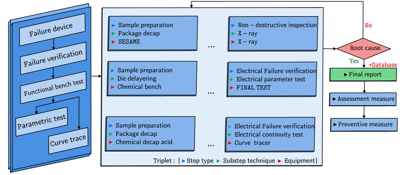
Figure 1: FRACAS: Structured representation of the failure analysis process. A failure description take indistinct failure analysis flow (path) to finding the root cause of the failure (Ezukwoke et al.,, 2021).

An important part of FRACAS is the final report (database) containing details of failure analyses and different combinations of FA. It is important to note that a failure description may have more than one failure analysis path leading to the same finding of the root cause. In fact, one failure description may have two different path with the same sequence of step type and substep technique but only differing in the analysing equipment.
Failure description (FDR). This is a free-text language encoding describing the type and context of failure observed on a microelectronic component or a semiconductor device. Given that free-text from FRACAS report contains lexical and technical jargons, symbolic imputations, abbreviations and numerous language encoding (due to the different geographical locations of the FA-expert); it becomes necessary to preprocess them into tokens understandable by machines using natural language processing techniques before modeling. Similar preprocessing pipeline proposed by Ezukwoke et al., (2021) for FRACAS data (Figure (1b)) for unsupervised modeling is adopted in this paper.
Failure Analysis Triplets (FATs). A series of Step type, Substep technique and equipment proposed by a failure analyst in order to find the root cause of a failure and propose a corrective action. The number of failure analysis triplets proposed by a failure analyst (expert) depends on the FDR and the available equipment. Depending on the failure description and available expertise and equipment, different length of FA can be proposed (See Figure 2). The FRACAS database, contains a description, and empty space padded failure analysis associated with the FDR. The padding is based on the longest failure analysis triplets.
Failure Analysis Triplets Generation (FATG). This is a scientific process of generating a series of sequential failure analysis text associated with a failure description. We model the FATG as a sequence-to-sequence data-to-text problem where the input is the FDR (structured tabular data), and the output is a long sequence of a failure analysis triplets. Data-to-text generation is commonly described as a task of automatically producing non-contextual, non-linguistic inputs (Gatt and Krahmer,, 2018). Early methods apply knowledge-based expert systems (Kukich,, 1983) for automatically generating natural language reports from computer databases; while recent generation techniques train end-to-end auto-encoding (encoder-decoder) architectures (Bahdanau et al.,, 2015) for similar purpose. Encoder-decoder framework are sequence-to-sequence (Seq2Seq) deep learning-based modeling technique employed in Long-Short-Term Memory (LSTM) (Liu et al.,, 2016; Prajit Ramachandran,, 2016; McCann et al.,, 2017) and Transformers (Vaswani et al.,, 2017) for natural language generation (NLG). In later sections of this paper, we explore language models, in particular, pre-trained language models based on Transformer architecture for FATG. We evaluate the performance of the different models using the popular scoring metrics like BLEU, ROUGE and METEOR. We first formalize our problem in a probabilistic graphical setting before extending it to language modeling.
Formalization.

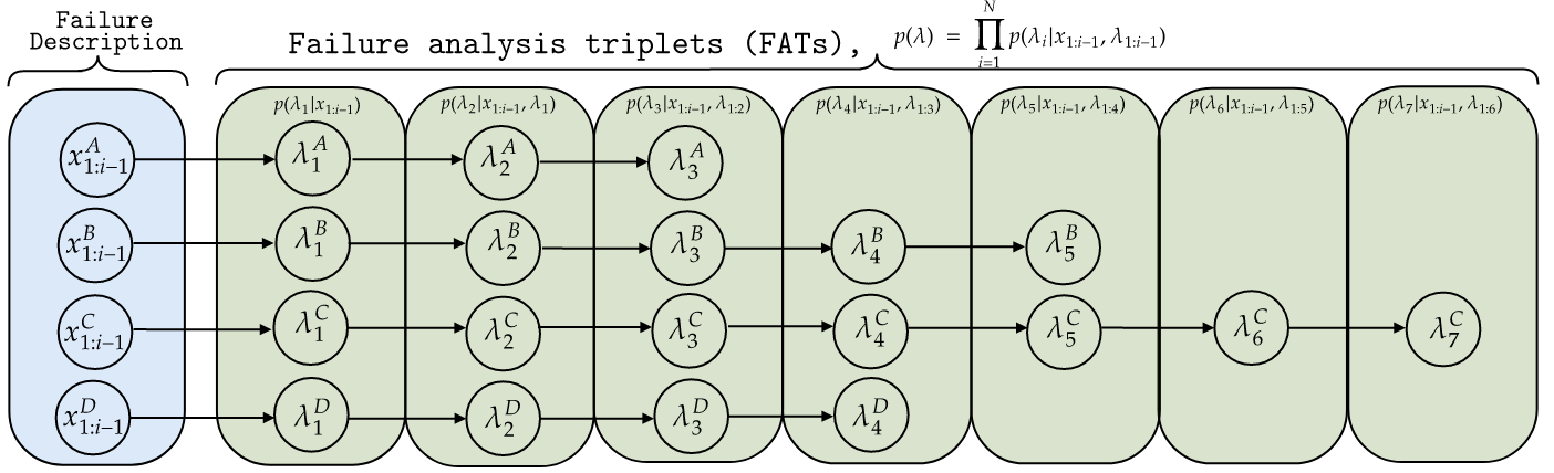
Figure 2: Failure analysis decision flow graphical formalization. A, B, C and D are different failure description with different failure analysis triplets length.

Given failure analysis description (FDR) $\{x_{i}\}_{i=1}^{N}\in\mathbb{R}^{D}$, where N is the number of observation and D is the dimension of the preprocessed data, and a set of failure analysis triplets $\{\lambda_{i}\}_{i=1}^{N}\in\mathbb{R}^{M}$, where $M$ is the dimension of $\lambda$. We express the FATG as data-to-text problem by defining the input space as a joint space of $x$ and $\lambda$. Let us begin by modeling them individually, the FDR (input space) probability mass function is,

$$p_{x}(x)=\prod_{i=1}^{N}p_{x}(x_{i}|x_{1:i-1})$$ (1)

and the failure analysis triplets (FAT),

$$p_{\lambda}(\lambda)=\prod_{i=1}^{N}p_{\lambda}(\lambda_{i}|\lambda_{1:i-1})$$ (2)

The joint probability space is given as,

$$p_{x,\lambda}(x,\lambda)=\prod_{i=1}^{N}p_{x,\lambda}(\lambda_{i}|x_{1:i-1},\lambda_{1:i-1})$$ (3)

Compact representation. We present a compact representation for Equation (3) as follows. Let us represent the joint space between failure description $x\in\mathbb{R}^{D}$ and failure analysis triplets $\lambda\in\mathbb{R}^{M}$ i.e $\{x_{i},\lambda_{i}\}_{i=1}^{N}\in\mathbb{R}^{K}$ as $\Lambda\in\mathbb{R}^{K}$ , where $K=D+M$ is the dimension of the joint space- a sum of the dimensions of $x$ and $\lambda$ respectively.. We define the compact joint probability space between $x$ and $\lambda$ as,

$$p(\Lambda)=\prod_{i=1}^{N}p(\Lambda_{i}|\Lambda_{1:i-1})$$ (4)

This compact joint space can be modeled into a likelihood function, $\sum_{i=1}^{N}\log p(\Lambda_{i}|\Lambda_{1:i-1};\phi)$ and its parameter, $\phi$ estimated using deep neural network used in training pre-trained language models.

1.2 Pretrained Language Models (PLMs)

Interesting developments in deep learning domains resulting from the ability to effectively train models with large parameters has increased rapidly over time. One of the reasons for this is the access to innovative high computing clusters. Large datasets containing millions of observations (with similar or larger number of tokens) is needed to fully train model parameters and prevents overfitting. However, building large-scale labeled datasets can be computational expensive even for a high resource computing cluster for most NLP tasks due to the annotation costs. Pre-trained Model is originally introduced by Dai and Le, (2015) for NLP; Liu et al., (2016) as a shared LSTM encoder with Language Model (LM) for multi-task learning (MTL) using fine-tuning; Prajit Ramachandran, (2016) for unsupervised pre-training of Seq2Seq model and McCann et al., (2017) as a deep LSTM encoder from Seq2Seq model with machine learning.

Since large-scale unlabeled corpora require less computing resources, annotations is not usually needed or relatively easy to construct. Hence, to leverage the huge unlabeled text data, we can first learn a good representation from unlabelled corpora and then use these representations for other downstream tasks. Advantages of such pre-training methods include: (i) Learning universal language representations given their large access to tokens and using them for downstream tasks (such as done here for FATG); (ii) better initialization leading to better generalization on transfer learning; (iii) helps to avoid overfitting on small token data. Recent studies have demonstrated significant performance gains on many NLP tasks with the help of the representation extracted from the PLMs on the large unannotated corpora.

Given that most PLMs have relied greatly on Recurrent Neural Network (RNN) architectures such as Long-Short Term memory (LSTM) (Melis et al.,, 2018; Merity et al.,, 2017; Conneau et al.,, 2017) and Gated Recurrent Neural Network (GRNN) (Chaturvedi et al.,, 2017), it is impossible to ignore their significance for language generation task (Wen et al.,, 2015). RNNs make output predictions at each time step by computing a hidden state vector $H_{t}$ based on the current input token and the previous states. However, because of their auto-regressive property of requiring previous hidden states vectors $H_{t-n}$ (where $n$ is all hidden states vectors until $t$) to be computed before the current time step, $t$, they require a large amount of time and memory which can be unbearable. The problem with RNN based models is their inability to adapt to long sequence tasks rising from their lack of attention to previously seen sequences; they are computationally demanding and do not benefit from parallelization. As a result, Transformer models (Vaswani et al.,, 2017) which is built on a Self-attention Vaswani et al., (2017) (also an auto-regressive mechanism) is preferred over RNNS. They rely on dot-products between elements of the input sequence to compute a weighted sum (Lin et al.,, 2017; Ahmed et al.,, 2017; Bahdanau et al.,, 2014; Kim et al.,, 2017) which serves as a critical ingredient in natural language generation tasks. The Table (1) below shows a list of state-of-the-art pre-trained models built on LSTM and Transformers architectures together with the size of trainable parameters they were trained on.

Architecture	Model name	Params	Project source code
LSTM	LM-LSTM (Dai and Le,, 2015)		https://github.com/frankcgq105/BERTCHEN
	Shared LSTM (Liu et al.,, 2016)		https://github.com/afredbai/text_classification
	ELMo (Peters et al.,, 2018)		https://github.com/dmlc/gluon-nlp
	CoVE (McCann et al.,, 2017)		https://github.com/salesforce/cove
Transformer Encoder	BERT (L) (Devlin et al.,, 2019)	$340$M	https://github.com/google-research/bert
	SpanBERT (Joshi et al.,, 2020)	$340$M	https://github.com/mandarjoshi90/coref
	XLNet (L) (Yang et al.,, 2019)	$360$M	https://github.com/zihangdai/xlnet
	RoBERTa (Liu et al., 2019a, )	$356$M	https://github.com/facebookresearch/fairseq
Transformer Decoder	GPT (Radford and Narasimhan, 2018a, )	$117$M	https://github.com/huggingface/transformers
	GPT-2 (Radford et al.,, 2019)	$1.5$B	https://github.com/huggingface/transformers
	GPT-3 (Brown et al.,, 2020)	$175$B	https://github.com/huggingface/transformers
Transformer	MASS (Song et al.,, 2019)	$213$M	https://github.com/microsoft/MASS
	BART (Lewis et al.,, 2019)	$380$M	https://github.com/huggingface/transformers
	T5 (Raffel et al.,, 2020)	$11$B	https://github.com/huggingface/transformers
	XNLG (Chi et al.,, 2020)		https://github.com/CZWin32768/XNLG
	mBART (Liu et al.,, 2020)	$380$M	https://github.com/huggingface/transformers

Table 1: Pre-trained Language architectures well established for performing generative task.
XNLG: Unspecified parameter size in the original paper. Pre-trained on $10$-hidden encoder layers and $6$-hidden decoder layers with same model parameters as Transformer (Vaswani et al.,, 2017).

In general, pre-trained language models are classified into three taxonomies according to Qiu et al., (2020) and they include: (i) Representation: based on contextual or non-contextual representation of downstream task; (ii) Architectures: including LSTM, Transformer (standard encoder-decoder transformer), Transformer encoder (only encoder part of Transformer), Transformer decoder (only decoder part of Transformer); (iii) Pre-training tasks: Supervised learning (learning hypothesis/function that maps input to output), Unsupervised learning (finding clusters or latent representation in unlabelled data); Self-supervised learning (combining supervised and unsupervised learning but by first generating training labels automatically).
Encoder Pre-training. Encoder pre-training are bi-directional or auto-encoding model that only use encoder during pretraining. Pre-training in this setting is achieved by masking words in the input sentence while training the model to reconstruct. At each stage during pretraining, attention layers can access all the input words. This family of models, for instance BERT (Devlin et al.,, 2019) and XLNet (Yang et al.,, 2019), are most useful for tasks that require understanding complete sentences such as sentence classification or extractive question answering. See Table (1) for other Encoder pre-training examples.
Decoder Pre-training. often referred to as auto-regressive models, for example, GPT (Radford et al.,, 2019), use only the decoder during a pretraining that is usually designed so that the model predict the next words. The attention layers can only access the words positioned before a given word in the sentence, hence, their use for text generation task.

2 Language Modeling (LM)

Language Models (LMs), sometimes referred to as Unidirectional or auto-regressive LMs is a probabilistic density estimation approach to solving unsupervised NLP task (such as text generation). Given a text sequence $\{x_{i}\}_{i=1}^{N}\in\mathbb{R}^{D}$, its probability density mass $p(x)$ can be expressed as,

$$p(x)=\prod_{i=1}^{N}p(x_{i}|x_{0:i-1})$$ (5)

Where $x_{0}$ indicates the beginning of the sequence (usually a special token such as $<|\texttt{startoftext}|>$). The conditional probablity can be modeled using a probability distribution over $x_{i}$ given contextual tokens $x_{0:i-1}$. The contextual tokens can be modeled using neural encoder encoder as follows:

$$p(x_{i}|x_{0:i-1})=\texttt{softmax}(\texttt{encoder}(x_{0:i-1}))$$ (6)

Note that the softmax function can be any prediction function that fits the expectation and the final hidden layer- encoder can be self-masked decoder. We proceed with training the network with maximum likelihood estimate as follows:

$$\mathcal{L}_{LM}=\sum_{i=1}^{N}\log p(x_{i}|x_{0:i-1};\theta)$$ (7)

Where $\theta$ is the vector of parameters of the neural network. Other versions of losses are available to training the network depending on the user preference and problem description (See Qiu et al., (2020)).

2.1 Transformer Neural Network

Transformer network Vaswani et al., (2017) uses an encoder-decoder architecture with each layer consisting of an attention mechanism called multi-head attention, followed by a feed-forward network. From the source tokens, learned embedding of dimension $d_{model}$ are generated which are then modified by an additive positional encoding (PE).
Position Embedding (PE) is computed using the word position (pos) in the sentence and the dimension of the word vector as follows:

$$PE(pos,2i)=\texttt{sin}(\texttt{pos}/10000^{2i/d_{\texttt{model}}})$$ (8)

$$PE(pos,2i+1)=\texttt{cos}(\texttt{pos}/10000^{2i/d_{\texttt{model}}})$$ (9)

The PE corresponds to a sinusoidal wave with wavelength forming a geometric progression between $2\pi-10000\cdot 2\pi$ to allow the model learn relative positions.
Scaled Dot-Product Attention. A multi-head attention mechanism builds upon scaled dot-product attention, which operates on a query $Q$, key $K$ and a value $V$:

$$Attention(Q,K,V)=\texttt{softmax}\left(\frac{QK^{T}}{\sqrt{d_{k}}}\right)V$$ (10)

Where $d_{k}$ is the dimension of the key. The input are concatenated in the first layer so that each $(Q,K,V)$ form the word vector matrix. Multi-head attention mechanisms obtain $h$ different representations of $(Q,K,V)$, compute scaled dot-product attention for each representation, concatenate the results, and project the concatenation with a feed-forward layer.

$$head_{i}=\texttt{Attention}(QW_{i}^{Q},KW_{i}^{K},VW_{i}^{V})$$ (11)

$$MultiHead(Q,K,V)=\texttt{Concat}(head_{1},\dots,head_{h})W^{O}$$ (12)

Where $W_{i}$ and $W^{O}$ are the learned projection parameters, $W_{i}^{Q},W_{i}^{K}\in\mathbb{R}^{d_{model}\times d_{k}}$, $W_{i}^{V}\in\mathbb{R}^{d_{model}\times d_{v}}$, $W^{O}\in\mathbb{R}^{hd_{v}\times d_{model}}$ and $h$ denotes the number of heads in the multi-attention. $d_{v}$ is the dimension of the values. Vaswani et al., (2017) employs $h=8$ parallel attention layers (heads) and set $d_{k}=d_{v}=d_{model}/h=64$ to achieve the same computational cost as using single-head attention.
Position-wise Feed-Forward Networks (PFFN). The component of each layer of the encoder- decoder network is a fully connected feed-forward network applied to each position separately and identically. The authors propose using a two-layered network with a ReLU activation. Given trainable weights $W_{1},W_{2},b_{1},b_{2}$, the sub-layer is defined as:

$$FFN(x)=\texttt{max}(0,xW_{1}+b_{1})W_{2}+b_{2}$$ (13)

The proposed dimensionality of input and output is $d_{model}=512$, and the inner-layer has dimensionality $d_{ff}=2048$ (Vaswani et al.,, 2017).

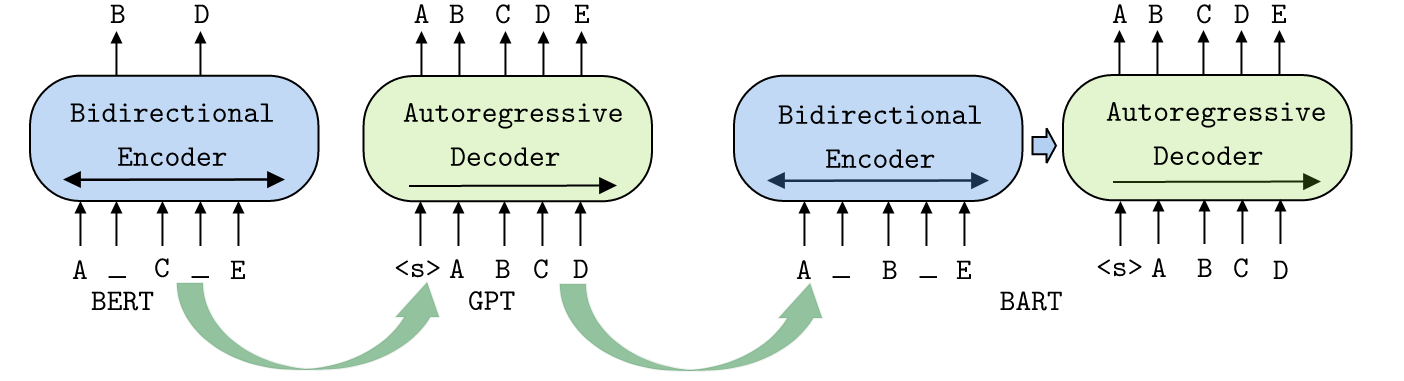
Figure 3: BERT: Random tokens are replaced with masks, and the document is encoded bidirectionally. Missing tokens are predicted independently. GPT: Tokens are predicted auto-regressively, meaning GPT can be used for generation. However words can only condition on leftward context, so it cannot learn bidirectional interactions. BART: Inputs to the encoder need not be aligned with decoder outputs, allowing arbitrary noise transformations. Here, a document has been corrupted by replacing spans of text with mask symbols. The corrupted document (left) is encoded with a bidirectional model, and then the likelihood of the original document (right) is calculated with an auto-regressive decoder (Lewis et al.,, 2019).

2.2 Generative Pre-trained Transformer (GPT) model

Generative Pre-training model (Radford and Narasimhan, 2018b, ) is a type of transformer model that uses a multi-layer Transformer decoder (Liu et al.,, 2018) instead of the encoder-decoder model introduced by Vaswani et al., (2017). The model structure begins with training in an unsupervised setting corpus of tokens $\mathcal{U}=\{u_{1},\dots,u_{n}\}$ with a standard likelihood objective to maximize:

$$L_{1}(\mathcal{U})=\sum_{i}logP(u_{i}|u_{i-k},\dots,u_{i-1};\Theta)$$ (14)

Where $k$ is the context window and $\Theta$ is the neural network parameters obtained when modeling conditional probability P. This model applies a multi-headed self-attention operation over the input context tokens followed by position-wise feed-forward layers to produce an output distribution over target tokens as follows:

$$h_{0}=UW_{e}+W_{p}$$ (15)

$$h_{i}=\texttt{transformer\_block}(h_{i-1})\quad\forall i\in[1,n]$$ (16)

$$P(u)=\texttt{softmax}(h_{n}W_{e}^{T})$$ (17)

Where $U=(u_{-k},\dots,u_{-1})$ is the context vector of tokens, $n$ here is the number of layers while $W_{e}$ and $W_{p}$ are the token embedding and position embedding matrix respectively. The results on our data for FATG shows that GPT models outperformed other models and the baseline model by over $100\%$ on BLEU score.

2.3 BART (Bidirectional Auto-Regressive Transformer)

model BART is a Bidirectional Auto-Regressive Transformer trained by (1) corrupting text with an arbitrary noising function, and (2) learning a model to reconstruct the original text (Lewis et al.,, 2019). BART uses a standard Transformer-based neural machine translation architecture (i.e Encoder-Decoder Transformer as seen in Figure 3). The BART loss function, $\mathcal{L}_{2}(\mathcal{U})$, used to train the pre-trained model is the negative log likelihood of the original training documents:

$$L_{2}(\mathcal{U})=-\sum_{i}logP(u_{i}|u_{i-k},\dots,u_{i-1};\Theta)$$ (18)

Note that the corpus of tokens $\mathcal{U}=\{u_{1},\dots,u_{n}\}$ is as seen for GPT while $\Theta$ is the neural network parameters.

2.4 PLMs for Failure analysis generation domain task

Despite the overwhelming performance of PLMs on opensource datasets, adapting them to domain specific downstream task can be challenging and sometimes futile. This under-generalization to downstream domain specific task is most often related to transfer learning issues. Transfer learning (Pan and Yang,, 2010) is the ability of a model to transfer the knowledge acquired from a source domain (task) to another domain (often called the target). The inability of PLMs to generalize arise from one or more key factors including: (i) Model architecture not fit for the downstream target domain; (ii) The data distribution of the target domain is far from the source domain on which the PLMs is trained. The later arises, when sufficient domain-specific knowledge for instance, tokens, sentence or characters combination learnt by the PLMs are lacking in the target domain, posing a huge semantic gap.

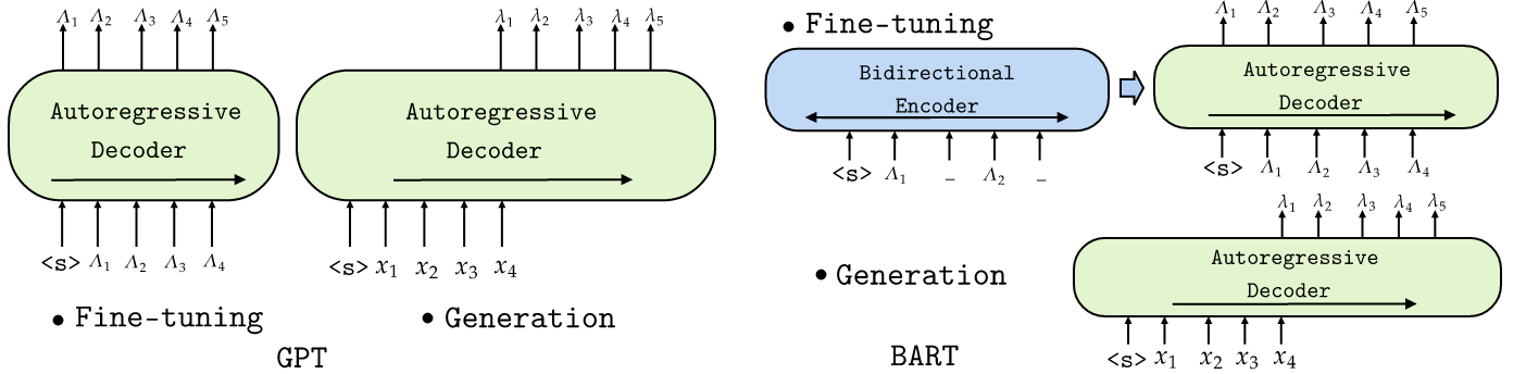
Figure 4: PLM for Failure analysis triplet generation (FATG). Both GPT and BART architecture are trained on joint input space $\{x,\lambda\}\in\Lambda$. Only the failure description (FDR) is the required input for generation.

We apply the weights of the PLMs to our task of failure analysis triplets generation (FATG) using the two transformer models described in previous sections (2.2, 2.3). Since, there are no labelled instance of FAT datasets, as they are confidential and unavailable from other domains, domain-adaptive intermediate fine-tuning (Phang et al.,, 2018) becomes a challenging task and hence, the poor performance on FATG task reported for GPT3 architecture and BERT (dropped due to lack of meaningful generation). It has been shown that the additional training with general-purpose text corpora (for example, WebText) on the same text generation task can improve the performance on a specific domain (Li et al.,, 2021). Interestingly, this is the case for GPT2 as it has been trained on WebText corpora, saving us time due intermediate fine-tuning. Results shows outstanding performance for all GPT2 models for the downstream FATG task.
We fine-tune the PLMs using the vanilla fine-tuning method as seen in DialogGPT (Zhang et al.,, 2019) for conversational response generation. The input and output data structures used for fine-tuning and generation are illustrated in the Figure (4) and maintain similar likelihood objective function used for pre-training for the fine-tuning phase.

3 Experiments

Setup. Experimentation is carried out on a High performance computing (HPC) cluster with 80 cores 2 $\times$ Intel Xeon E5-2698 v4 2.20GHz CPU (80 cores), $512$G RAM size and 8 $\times$ Nvidia V100 32G GPU.
miniature-GPT For our experiment, we maintain similar properties of the Transformer as proposed by Vaswani et al., (2017). The $d_{model},d_{v},d_{k}$ are the same. The model is trained for $100$ epochs. The maximum length of sequence is $80$, vocabulary size used is $20$K words, embedding size is $256$. Top-k (Holtzman et al., 2019a, ) decoding is used for generating the FA triplets.
Pre-trained GPT-2 & 3. We fine-tune three versions of the GPT-2 (gpt2, gpt2-medium ($335$M parameters), gpt2-large ($774$M-$1.5$B parameters)) for the purpose of failure analysis generation provided by the Huggingface API . The begin of sequence token, bos is set to $<|\texttt{startoftext}|>$; End of sequence token, eos, $<|\texttt{endoftext}|>$ and padding token, pad_token is $<|\texttt{pad}|>$. Batch size for training and evaluation is $1$; weight decay is $0.05$ and the number of training epochs is $100$. GPT2 is trained on $40$G of WebText data (web pages from outbound links on Reddit) excluding Wikipedia pages; the texts are tokenized using a byte-level version of Byte Pair Encoding (BPE) and contains a vocabulary size of $50257$. The inputs are sequences of $1024$ consecutive tokens. OPENAI-GPT3 ($175$B parameters and $500$B tokens) however was trained on BooksCorpus dataset (Zhu et al.,, 2015), which contains over $7000$ unique unpublished books from a variety of genres including Adventure, Fantasy, and Romance. GPT3 uses similar encoding as GPT2, a bytepair encoding (BPE) vocabulary with $40$K merges.
BART Model. The bos, eos, pad_token and tokenization (byte-pair encoding) are same with those used for GPT-2. We use the same pre-training data as Liu et al., 2019b , consisting of 160Gb of news, books, stories, and web text.

3.1 Dataset

We perform experimentation using real failure analysis data from a semiconductor industry, taking into account only successful failure analysis for one year (2019). In order to train the transformer model, we first concatenate all input features along the horizontal axis ($x-axis$) with the triplet data. The size of the data after preprocessing for one year ($2019$) is $5809$. The $10$-input failure description features (see Table 2) also called Expert features include: Reference, Subject, Site, Requested activity, Priority level, High confidentiality, Context, Objectives / Work description, Source of failure / request, Source of failure (Detailled) to train the Transformer model.

Feature	Description	Example
Reference	Concatenated tokens describing the failure analysis team, FA-lab, year and ID	PTM BOUSKOURA _18_04655
Subject	A unique subject particular to the fault expert desire to analyse	Load failure
Site	Failure analysis lab site	Grenoble
Requested activity	Major fault analysis requested by expert or client	Failure Analysis
Priority level	Level of priority given to failure device	P1, P2 or P3
High confidentiality	Confidentiality level	Yes or No
Context	Context reason for the failure analysis	Non-operational Heat Soak Fail
Objective/Work description	Objective of the failure analysis	Check possible cause of failure
Source of failure/Request	Entity that identified the failure	Customer Complaint
Source of failure (Detailed)	Details on the failure source	Reliability Failure

Table 2: Brief description of the input failure description (FDR) variables and their corresponding examples.

The features are concatenated along the horizontal axis with the FATs for Modeling. FATs has a dimension of $\mathbb{R}^{69}$ with the longest FA having $23$ triplets. We preprocess FDR, $x$ according to the scheme presented in Ezukwoke et al., (2021) and vectorize the joint space $\{x,\lambda\}$ using a byte-level version of Byte Pair Encoding (BPE) from GPT2.

3.2 Evaluation metric

BLEU (Bilingual Evaluation Understudy) is a context-free precision-based metric for evaluating the quality of text which has been machine-translated from one natural language to another (Papineni et al.,, 2002; Lin and Hovy,, 2003) and has also been adopted for dialog generation task (Sai et al.,, 2022). It is a precision-based metric that computes the n-gram overlap between the reference (original) and its hypothesis. In particular, BLUE is the ratio of the number of overlapping $n$-grams to the total number of $n$-grams in the hypothesis. It is formally defined as,

$$BLEU-N=\text{BP}\cdot exp\left(\sum_{n=1}^{N}\mathbf{w_{n}}\log Precision_{n}\right)$$ (19)

$\mathbf{w_{n}}$ is the weights of the different $n-grams$ and BP known as the brevity penalty is used to discourage short meaningless hypothesis,

$$BP=\begin{cases}1,&\text{if $|\texttt{hyp}|$}>|\texttt{ref}|\\ e^{\left(1-\frac{|\texttt{ref}|}{|\texttt{hyp}|}\right)}&\text{otherwise}\end{cases}$$ (20)

Where $|\texttt{ref}|$ and $|\texttt{hyp}|$ are the length of the reference and hypothesis respectively. Precision is defines as,

$$Precision_{n}=\frac{\sum_{p_{n}\in\texttt{hyp}}\sum_{\texttt{n-gram}\in p_{n}}Count_{clip}(\texttt{n-gram})}{\sum_{p_{n}\in\texttt{hyp}}\sum_{\texttt{n-gram}\in p_{n}}Count(\texttt{n-gram})}$$ (21)

Where $p_{n}$ is a subset of $n$-tokens in the hypothesis tokens and $\text{Count}_{clip}(n-gram)$ is the maximum number of times the given $n$-gram appears in any one of the corresponding reference sentences. In our case, we use it to compare the original expert triplet failure analysis to the Transformer generated triplets without respect to context. The average BLEU score (Avg-BLEU) is computed on a one-to-one basis (Expert triplets-to-Transformer triplets).
ROUGE (Recall-Oriented Understudy for Gisting Evaluation) (Lin,, 2004) is a recall-based metric similar to BLEU-N in counting the n-gram matches between the hypothesis and reference. It is computed as follows:

$$ROUGE-N=\frac{\sum_{s_{r}\in\texttt{ref}}\sum_{\texttt{n-gram}\in s_{r}}Count_{match}(\texttt{n-gram})}{\sum_{s_{r}\in\texttt{ref}}\sum_{\texttt{n-gram}\in s_{r}}Count(\texttt{n-gram})}$$ (22)

Where ref is the reference text and $s_{r}$ is the hypothesis summary. ROUGE-L is the F-measure of the longest common subsequence (LCS) between a pair of sentences. LCS(p, r) is the common subsequence in p and r with maximum length. ROUGE-L is computed as follows:

$$ROUGE-L=\frac{(1+\beta^{2})R_{LCS}P_{LCS}}{R_{LCS}+\beta^{2}P_{LCS}}$$ (23)

Where Precision,

$$P_{LCS}=\frac{|LCS(\texttt{ref},\texttt{hyp})|}{\text{Num. words in hypothesis}}$$ (24)

and Recall,

$$R_{LCS}=\frac{|LCS(\texttt{ref},\texttt{hyp})|}{\text{Num. words in reference}}$$ (25)

ROUGE-L is a matching and credible metric for the downstream task of failure analysis triplets generation task, as it does not take into account, contextual meaning but rather, word order and their maximum length. Its F-measure is highlighted to show its significance. The weight parameter $\beta^{2}$ emphasizes the precision as much as the recall.
METEOR proposed by Banerjee and Lavie, (2005) addresses the major drawback of BLEU including, inability to account for recall and inflexible $n$-gram matching by proposing an F-measure with flexible n-gram matching criteria. The F-measure is computed as follow:

$$F-score=\frac{10\text{Precision}\times\text{Recall}}{\text{Recall}+9\text{Precision}}$$ (26)

Where

$$Precision=\frac{\text{Num. mapped unigrams}}{\text{Num. unigrams in candidate}}$$ (27)

and

$$Recall=\frac{\text{Num. mapped unigrams}}{\text{Num. unigram in reference}}$$ (28)

METEOR tends to reward longer contiguous matches using a penalty term known as fragmentation penalty (Banerjee and Lavie,, 2005).

3.2.1 LESE: LEvenshtein Sequential Evaluation metric

For better understanding of the sequential generation of FATs and to address the drawback of ROUGE, we propose LEvenshtein Sequential Evaluation (LESE) metric. LESE is an $n$-gram Levenshtein distance (Levenshtein,, 1965) based metric used for measuring the similarity between two sequences by computing the $n$-gram edits (insertions, deletions or substitutions) required to change one sequence into another. It is unbiased in the computation of precision and recall as it takes into account the total number of $n$-grams as the denominator, in the computation of the precision and recall rather than unigrams. Given a reference sequence, ref$=a_{1},\dots,a_{m}$ and a hypothesis sequence, hyp$=b_{1},\dots,b_{n}$, where $m$ and $n$ are the length of ref and hyp respectively, the nonsymmetric $n$-gram Levenshtein distance (Lev) is given by the recurrence,

$$Lev_{(i,j)}(\texttt{r,h})=\begin{cases}Lev_{(i,0)}=\sum_{k=1}^{i}w(a_{k})\qquad\text{for }1\leq i\leq m\\ Lev_{(0,j)}=\sum_{k=1}^{j}w(b_{k})\qquad\text{for }1\leq j\leq n\\ Lev_{(i-1,j-1)}\qquad\qquad\text{for }a_{i:i+n-\text{gram}}=b_{j:j+n-\text{gram}}\\ 1+min\begin{cases}Lev_{\color[rgb]{1,0,0}d}(i-1,j)\\ Lev_{\color[rgb]{1,0,0}i}(i,j-1)\text{ for }a_{i:i+n-\text{gram}}\not=b_{j:j+n-\text{gram}}\\ Lev_{\color[rgb]{1,0,0}s}(i-1,j-1)\\ \end{cases}\end{cases}$$ (29)

$Lev_{(m,n)}(\texttt{r,h})=Lev_{(m,n)}(\texttt{r,h})//\texttt{n-gram}$ is the $n$-gram Levenshtein distance; r and h refer to the reference and hypothesis sequence while $Lev_{\color[rgb]{1,0,0}d}$, $Lev_{\color[rgb]{1,0,0}i}$ and $Lev_{\color[rgb]{1,0,0}s}$ denote the deletion, insertion and substitution operations. The smaller the Levenshstein distance between two sequences, the higher their similarity, hence, Lev(ref, hyp) = 0 when hyp = ref. The LESE-N (F1-score) is computed thus,

$$\textbf{LESE-N}=\frac{(1+\beta^{2})P_{\texttt{Lev}}R_{\texttt{Lev}}}{\beta^{2}P_{\texttt{Lev}}+R_{\texttt{Lev}}}$$ (30)

The value of $\beta$ in Equation (30) is $1$ for all experiments with Precision and Recall defined as follow,

$$\begin{cases}P_{\texttt{Lev}}=\texttt{max}\Bigl{\{}0,\left|\frac{|\texttt{max}(\texttt{|r|}_{\texttt{n-gram}},\texttt{|h|}_{\texttt{n-gram}})-\texttt{Lev}_{(m,n)}(\texttt{r, h})|}{\texttt{|n-gram in hypothesis|}}\right|\Bigl{\}}\\ R_{\texttt{Lev}}=\texttt{max}\Bigl{\{}0,\left|\frac{|\texttt{max}(\texttt{|r|}_{\texttt{n-gram}},\texttt{|h|}_{\texttt{n-gram}})-\texttt{Lev}_{(m,n)}(\texttt{r, h})|}{\texttt{|n-gram in reference|}}\right|\Bigl{\}}\\ \end{cases}$$ (31)

The numerators in Equation (31) is the length between the maximum $n$-grams in |ref| and |hyp|, and the Levenshstein distance, Lev(ref, hyp). Maximum is taken to avoid numerical problem that arise from empty sequence for either reference or hypothesis (as observed for FATG) or sometimes both.

When compared to human evaluation, LESE-N performs comparatively similar, especially LESE-3 for FATG compared to other metric used for quantitative evaluation.

3.3 Decoding method

Top-$k$ Sampling. Given a conditional probability distribution $p(x_{t}|x_{0:t-1})$, it top-$k$ vocabulary {$V:V^{k}\subset V$} is defined as the set of size -$k$ which maximizes the conditional probability $\sum_{x\in V^{k}}p(x_{t}|x_{0:t-1})$. At each time step, the top-$k$ possible next tokens are sampled according to their relative probabilities. The conditional distribution can be re-scaled thus,

$$p^{\prime}(x_{i}|x_{0:i-1})=\begin{cases}\frac{p(x_{i}|x_{0:i-1})}{\sum_{x\in V^{k}}p(x_{i}|x_{0:i-1})},&\text{if $x_{i}$}\in V^{k}\\ 0,&\text{otherwise}\end{cases}$$ (32)

and then sampling on the re-scaled probabilities.
Nucleus Sampling (Holtzman et al., 2019b, ). Given a conditional probability distribution $p(x_{t}|x_{0:t-1})$, the top-$p$ vocabulary {$V:V^{p}\subset V$} is denoted by,

$$\sum_{x\in V^{p}}p(x_{i}|x_{0:i-1})\geq p_{i}$$ (33)

Where $p_{t}$ is a user defined threshold taking values between $[0,1]$. otherwise known as top-$p$, nucleus sampling is a stochastic decoding sampling method that uses the shape of a probability distribution to determine the set of tokens to sample from. It avoids text degeneration by truncating the tail of the probability distribution. Furthermore, it resolves the challenge of flat and peaked-distribution faced when using top-$k$ by re-scaling the distribution $p(x_{t}|x_{0:t-1})$ from which the next token is sampled as,

$$p^{\prime}(x_{i}|x_{0:i-1})=\begin{cases}\frac{p(x_{i}|x_{0:i-1})}{\sum_{x\in V^{p}}p(x_{i}|x_{0:i-1})},&\text{if $x_{i}$}\in V^{p}\\ 0,&\text{otherwise}\end{cases}$$ (34)

The size of the sampling set will adjust dynamically based on the shape of the probability distribution at each time-step (Holtzman et al., 2019b, ).

4 Results

4.1 Quantitative Evaluation

We evaluate the performance of PLMs for Failure analysis generation (FATG). Evaluating the generative power of a model requires an equally optimized decoding method. We combine top-$p=0.95$ and top-$k=10$ with a normalizing temperature value of $1.9$ for decoder sampling of pretrained BART, GPT2, GPT2-Medium, GPT2-Large and OPENAI-GPT3 models. Top-$k$ (with $k=10$) performs well for the generative decoder sampling of mini-GPT.

				ROUGE-1			ROUGE-L			LESE-1				LESE-3
Model	BLUE-1	BLEU-3	MET.	Prec.	Rec.	F1	Prec.	Rec.	F1	Prec.	Rec.	F1	Lev-1	Prec.	Rec.	F1	Lev-3
mini-GPT	11.54	7.51	34.61	11.22	16.12	12.63	10.19	14.79	11.52	8.11	8.57	7.11	46.69	0.38	0.27	0.30	16.0
BART†	6.14	4.71	9.23	11.24	10.79	10.16	10.40	10.06	9.43	5.26	4.04	4.08	42.71	1.68	1.29	1.28	14.0
GPT3†	6.10	2.30	30.69	7.07	13.49	8.84	6.29	12.22	7.91	4.10	9.83	5.46	82.16	0.41	0.63	0.42	28.0
GPT2†	22.18	17.39	29.71	30.25	33.79	29.67	28.35	31.62	27.75	22.04	23.99	20.97	42.26	11.03	11.99	10.49	15.0
GPT2-M†	22.15	17.32	30.38	29.89	34.36	29.69	27.97	32.20	27.78	21.97	24.81	21.21	43.28	11.10	12.56	10.74	15.0
GPT2-L†	22.46	17.60	30.79	29.73	34.77	29.82	27.86	32.63	27.93	21.88	24.91	21.25	43.41	11.04	12.56	10.73	16.0

Table 3: Model comparison on BLEU (Papineni et al.,, 2002), ROUGE-1 & L (Lin,, 2004) and METEOR (MET.) (Banerjee and Lavie,, 2005) scores (%). Higher values (in bold-blue) is preferred for all metric except Lev (average $n$-gram Levenshstein distance). GPT2-L (Large) and GPT2-M (Medium) are both competitive in performance with Large, averagely performing better on BLEU, ROUGE and LESE scores compared to baseline (mini-GPT). GPT2-M performs best on LESE-3 triplet score, closely followed by GPT2-L. Prec. Rec; and F1 denote Precision, Recall and F1-score respectively. {Model}^†: Pre-trained model.

Results (as seen on Table 3) indicates GPT2-Model trained on the Webtext dataset performs considerably better than the baseline (mini-GPT), GPT3 and BART models. The best peforming GPT2 (GPT2 Large) outperforms the base model by $49\%$ on the BLEU metric; $73\%$ better than BART and GPT3 for FATG. The LESE metric evidently shows that GPT2, GPT2 Medium and GPT2 Large is trained on correlating domain knowledge related to failure analysis and reliability engineering, hence, the adaptive transfer of knowledge for failure analysis triplets generation.

					ROUGE-1			ROUGE-L			LESE-1				LESE-3
Weight	Year	BLUE-1	BLEU-3	MET.	Prec.	Rec.	F1	Prec.	Rec.	F1	Prec.	Rec.	F1	Lev-1	Prec.	Rec.	F1	Lev-3
$w^{\dagger}$	2019	22.15	17.32	30.38	29.89	34.36	29.69	27.97	32.20	27.78	21.97	24.81	21.21	43.28	11.10	12.56	10.74	15.0
$w_{2019}$	2020	21.64	17.16	29.70	27.99	34.31	28.32	26.39	32.47	26.69	21.59	24.73	21.02	41.96	11.21	12.89	10.96	15.0
$w_{2020}$	2021	24.02	18.32	31.71	31.59	35.98	31.71	29.69	33.83	29.79	22.20	24.83	21.57	45.06	10.57	12.03	10.32	16.0

Table 4: GPT2 Medium: Transfer learning model comparison across yearly FA data (year-$2020$ $\in\mathbb{R}^{5672\times 79}$; year-$2021$ $\in\mathbb{R}^{2906\times 79}$). The checkpoint weights from previous year (for instance, year 2019 is used for training year -$2020$ and so on). The marginal improvement in the LESE-3 scores for year-$2021$ suggests that the weight ($w_{2019}$), generalizes the sub-domains. Improvement in LESE-3 is not monotonic, observe the best scores (in bold-blue) for year-$2020$ and only slightly less for year-$2021$ due to insufficient learning data. $w^{\dagger}$: Fine-tuned pre-trained weight.

The best performing model on longest common triplets (LCT), related to longest common subsequence generation is GPT2 Medium and Large. Both ROUGE-L and METEOR favor long sequence triplet generation. Similarly, GPT2 Medium, measures up in performance with GPT2 Large (in terms of ROUGE-L and METEOR). In the next section, where we compare the model FATG to expert (human) triplets, we show that the FATs generated by GPT2 Medium and GPT2 Large are not differentiable.

4.2 Qualitative Evaluation: FATG

The quality of FATG of a model depends on its ability to adapt previously seen source domain knowledge to downstream domain task (at training time) as well as the quality of prompt (at generation time). Well preprocessed training data ($\Lambda$) and prompt (failure description), $x$ are two of the major factors that can degrade the generative quality. We classify this generation difficulty into three classes (i) Short-sequence FATG (ii) Long-sequence FATG. Transformers-based PLMs are by default designed for long sequence generation and particularly perform well for generating contextual text and summarization task. We evaluate their performance for structured FATG and report our findings.

4.2.1 Short sequence FATG (SS-FATG)

FDR	failed abnormal thd analysis failure manufacturing axis customer limit complaint castelletto data
	FATs	LESE-1 (%)	LESE-3 (%)
FATs (Human)	$\blacktriangleright$ Others; administrative activity; OM113 - LEICA M165C $\blacktriangleright$ Non destructive Inspection; X-ray; PK103 - PHOENIX X-RAY NANOMEX $\blacktriangleright$ Electrical Failure Verification; Electrical parametrical test; ZZ003 - CRI7 $\blacktriangleright$ Electrical Failure Verification; Electrical parametrical test; ZZ002 - CRI6	100	100
mini-GPT	-	-	-
BART	$\blacktriangleright$ d abnormal thd $\blacktriangleright$ Physical Analysis; Optical inspection; ANALYSIS EQU EQUIPMENT $\blacktriangleright$ Others; administrative failed; thD403 $\blacktriangleright$ Others; administrative activity; FINAL REPORT GENERATION $\blacktriangleright$ Non destructive Inspection; Optical microscopy; LOW POWER SCOPE	0.00	0.00
GPT3	$\blacktriangleright$ sample preparation package; decap; tools $\blacktriangleright$ sample preparation; package decap; sp001 - wet + microscopio $\blacktriangleright$ physical analysis; sem; em202 - nvision 40 $\blacktriangleright$ others; administrative activity; om103 - leica dm lmp $\blacktriangleright$ others; administrative activity; om113 - leica m165c $\blacktriangleright$ non destructive inspection; ir microscopy; om111 - olympus mx51 - f $\blacktriangleright$ electrical failure verification; electrical parametrical test; zz003 - cri7 ( m202 $\blacktriangleright$ global fault localisation; emmi; failure rate chain chain analyzer ( ecn $\blacktriangleright$ global fault localisation; emmi; fi105 - s105 ) oem esafm01 $\blacktriangleright$ electrical failure verification; electrical parametrical test; fv001 - bench test $\blacktriangleright$ electrical failure verification; continuity test; ftracer - ecn 4	35.56	13.33
GPT2	$\blacktriangleright$ Others; administrative activity; OM113 - LEICA M165C $\blacktriangleright$ Non destructive Inspection; X-ray; PK103 - PHOENIX X-RAY NANOMEX $\blacktriangleright$ Electrical Failure Verification; Electrical parametrical test; FV001 - BENCH TEST	76.19	57.14
GPT2 Medium	$\blacktriangleright$ Others; administrative activity; OM113 - LEICA M165C $\blacktriangleright$ Non destructive Inspection; X-ray; PK103 - PHOENIX X-RAY NANOMEX $\blacktriangleright$ Electrical Failure Verification; Electrical parametrical test; ZZ003 - CRI7 $\blacktriangleright$ Electrical Failure Verification; Electrical parametrical test; ZZ002 - CRI6	100	100
GPT2 Large	$\blacktriangleright$ Others; administrative activity; OM113 - LEICA M165C $\blacktriangleright$ Non destructive Inspection; X-ray; PK103 - PHOENIX X-RAY NANOMEX $\blacktriangleright$ Electrical Failure Verification; Electrical parametrical test; FV001 - BENCH TEST	76.19	57.14

Table 5: SS-FATG. A comparison of the failure analysis generated for different models given a prompt with $4$-human expert FATs. GPT2-Medium performs the best in generating highly correlating FATs as the human expert with a perfect LESE-$1$ and LESE-$3$ scores.

FDR	fail fault support serial number isolation analysis failure lotid shenzhen engineering postda determine
	FATs	LESE-1 (%)	LESE-3 (%)
FATs (Human)	$\blacktriangleright$ Sample preparation; Wafer / Die Backside prep; SP120 - ALLIED TECHPREP $\blacktriangleright$ Sample preparation; Die Delayering; SP001 - WET+MICROSCOPIO $\blacktriangleright$ Non destructive Inspection; SEM; EM201 - LEO 1530 $\blacktriangleright$ Global fault localisation; Static Laser Techniques; FI105 - IPHEMOS-MP $\blacktriangleright$ Electrical Failure Verification; Continuity test; FV001 - BENCH TEST	100	100
mini-GPT	-	-	-
BART	$\blacktriangleright$ d abnormal thd anomaly failed thc abnormal parametric gnd amp $\blacktriangleright$ Sample preparation Package decap SP006 - MAN_LASER+WET+MICRO $\blacktriangleright$ Non destructive Inspection X-ray PK103 - PHOENIX X-RAY	16.67	0.00
GPT3	$\blacktriangleright$ sample preparation package decap tools $\blacktriangleright$ sample preparation; package decap; sp001 - wet + microscopio $\blacktriangleright$ physical analysis; sem; em202 - nvision 40 $\blacktriangleright$ others; administrative activity; om103 - leica dm lmp $\blacktriangleright$ others; administrative activity; om113 - leica m165c $\blacktriangleright$ non destructive inspection; ir microscopy; om111 - olympus mx51 - f $\blacktriangleright$ electrical failure verification; electrical parametrical test; zz003 - cri7 $\blacktriangleright$ global fault localisation; static laser techniques; fi105 - iphemos $\blacktriangleright$ global fault localisation; emmi; emmi obirch ch $\blacktriangleright$ electrical failure verification; electrical parametrical test; fv001 - bench test	0.00	0.00
GPT2	$\blacktriangleright$ rejects shz obirch pocutornplgattransport $\blacktriangleright$ Sample preparation; Die Delayering; PARALLEL LAPPING-ECN6432 $\blacktriangleright$ Physical Analysis; SEM; FIB/SEM $\blacktriangleright$ Physical Analysis; FIB Cross Section; FIB/SEM $\blacktriangleright$ Non destructive Inspection; Optical microscopy; METALGRAPHIC MICROSCOPE MX61 $\blacktriangleright$ Global fault localisation; Static Laser Techniques; EMMI OBIRCH $\blacktriangleright$ Global fault localisation; EMMI; EMMI OBIRCH $\blacktriangleright$ Electrical Failure Verification; Electrical parametrical test; BENCH TEST	30.77	0.00
GPT2 Medium	$\blacktriangleright$ Sample preparation; Package decap; TOOL DECAP $\blacktriangleright$ Physical Analysis; SEM; FIB/SEM $\blacktriangleright$ Physical Analysis; FIB Cross Section; FIB/SEM $\blacktriangleright$ Non destructive Inspection; Optical microscopy; METALGRAPHIC MICROSCOPE MX61 $\blacktriangleright$ Global fault localisation; Static Laser Techniques; EMMI OBIRCH $\blacktriangleright$ Electrical Failure Verification; Continuity test; CURVE TRACER 1	36.36	0.00
GPT2 Large	$\blacktriangleright$ Sample preparation; Package decap; TOOL DECAP $\blacktriangleright$ Physical Analysis; SEM; FIB/SEM $\blacktriangleright$ Physical Analysis; FIB Cross Section; FIB/SEM $\blacktriangleright$ Non destructive Inspection; Optical microscopy; METALGRAPHIC MICROSCOPE MX61 $\blacktriangleright$ Global fault localisation; Static Laser Techniques; EMMI OBIRCH $\blacktriangleright$ Global fault localisation; EMMI; EMMI OBIRCH $\blacktriangleright$ Electrical Failure Verification; Electrical parametrical test; BENCH TEST	27.78	0.00

Table 6: SS-FATG. A comparison of the failure analysis generated for different models given a prompt with $5$-human expert FATs. LESE-3 scores for this FDR is null indicating the absence of correlating triplets with human FATs. GPT-2 Medium LESE-1 scores outperform other models signaling quality generation of step types and substep techniques.

FDR	result serial pras visual assembly coppell cse stated field ale preanalysis michael incident passivation dodge comm stmicroelectronics required material eos scott customer segment production belvidere conti ppm final failure registration hole supplier complaint chr relevant cseale shorted severirty analyst product standard analysis ecu type location inspection vin mileage quantity warranty subtype
	FATs	LESE-1 (%)	LESE-3 (%)
FATs (Human)	$\blacktriangleright$ Physical Analysis; Optical inspection; ANALYSIS EQUIPMENT $\blacktriangleright$ Physical Analysis; Optical inspection; HIGH POWER SCOPE $\blacktriangleright$ Physical Analysis; Optical inspection; LOW POWER SCOPE	100	100
mini-GPT	-	-	-
BART	$\blacktriangleright$ d abnormal thd $\blacktriangleright$ Physical Analysis; Optical inspection; ANALYSISIS EQUIPMENT $\blacktriangleright$ Others; administrative; failed tht abnormal observed mud abnormal $\blacktriangleright$ Inspection; Optical inspection; HIGH POWER failed STd abnormal $\blacktriangleright$ Non destructive Inspection; Optical microscopy; LOW POWER SCOPE	19.05	0.00
GPT3	$\blacktriangleright$ sample preparation; package decap; tools $\blacktriangleright$ sample preparation; package decap; sp001 - wet + microscopio $\blacktriangleright$ physical analysis; sem; em202 - nvision 40 $\blacktriangleright$ others; administrative activity; om103 - leica dm lmp $\blacktriangleright$ non destructive inspection; ir microscopy; om111 - olympus mx51 - f $\blacktriangleright$ electrical failure verification; electrical parametrical test; fv001 - bench test $\blacktriangleright$ global fault localisation; emmi; fibsem $\blacktriangleright$ global fault localisation; emmi; analyzer $\blacktriangleright$ global fault localisation; emmi; lsm electrical failure verification	5.56	0.00
GPT2	$\blacktriangleright$ signature andorch conditions huawei $\blacktriangleright$ Physical Analysis; Optical inspection; LSM $\blacktriangleright$ Physical Analysis; Optical inspection; L200 MICROSCOPE 2 $\blacktriangleright$ Others; administrative activity; FINAL REPORT GENERATION $\blacktriangleright$ Global fault localisation; Static Laser Techniques; LSM	34.78	0.00
GPT2 Medium	$\blacktriangleright$ conti severirty preanalysis final coppell $\blacktriangleright$ Sample preparation; Package decap; CHEMICAL HOOD $\blacktriangleright$ Sample preparation; Package decap; LASER DECAPPER $\blacktriangleright$ Physical Analysis; Optical inspection; L200 MICROSCOPE 2 $\blacktriangleright$ Physical Analysis; Optical inspection; NIKON STEREO MICROSCOPE IN CPL FA $\blacktriangleright$ Others; administrative activity; FINAL REPORT GENERATION	30.77	0.00
GPT2 Large	$\blacktriangleright$ conti cseale $\blacktriangleright$ Sample preparation; Package decap; CHEMICAL HOOD $\blacktriangleright$ Sample preparation; Package decap; LASER DECAPPER $\blacktriangleright$ Physical Analysis; Optical inspection; L200 MICROSCOPE 2 $\blacktriangleright$ Physical Analysis; Optical inspection; NIKON STEREO MICROSCOPE IN CPL FA $\blacktriangleright$ Others; administrative activity; FINAL REPORT GENERATION	33.33	0.00

Table 7: SS-FATG. A comparison of the failure analysis generated for different models given a prompt with $3$-human expert FATs. GPT2 performs the best in generating high correlating FATs as the human expert.

Given a FDR prompt and a short human-expert failure analysis triplets (with length ranging between $3-6$), Short sequence FATG (SS-FATG) is the ability of a fine-tuned PLM to generate the same order and length of the FATs given by human-expert. Short sequence FATs (SS-FATs), can be partial incomplete FA that compliments a main FA. We observe from generation task, that all the models including mini-GPT (non-pretrained baseline), BART, GPT2 (base), GPT2 Medium and GPT2 Large are capable of generating short sequences. However, PT-BART generates incorrect SS-FATs while GPT3 generates mostly long sequence with low BLEU and LESE scores. GPT3 is modeled with the objective of generating long sequences for story-telling, hence, its behaviour during FATG. We give an illustration of a case of SS-FATG task using the best result from GPT2 and a much lesser BART generation result.
Short sequence FATG (SS-FATG)
FDR prompt: failed abnormal thd analysis failure manufacturing axis customer limit complaint castelletto data
Human FATs:
$\blacktriangleright$ Others; administrative activity; OM113 - LEICA M165C
$\blacktriangleright$ Non destructive Inspection; X-ray; PK103 - PHOENIX X-RAY NANOMEX
$\blacktriangleright$ Electrical Failure Verification; Electrical parametrical test; ZZ003 - CRI7
$\blacktriangleright$ Electrical Failure Verification; Electrical parametrical test; ZZ002 - CRI6
GPT2-M FATs: BLEU-3: $100.00\%$ LESE-3: Prec.: $100.00\%$ Rec.: $100.00\%$ F1.: $100.00\%$
$\blacktriangleright$ Others; administrative activity; OM113 - LEICA M165C
$\blacktriangleright$ Non destructive Inspection; X-ray; PK103 - PHOENIX X-RAY NANOMEX
$\blacktriangleright$ Electrical Failure Verification; Electrical parametrical test; ZZ00 3 - CRI7
$\blacktriangleright$ Electrical Failure Verification; Electrical parametrical test; ZZ002 - CRI6
BART FATs: BLEU-3: $0.00\%$ LESE-3: Prec.: $0.00\%$ Rec.: $0.00\%$ F1.: $0.00\%$
$\blacktriangleright$ d abnormal thd
$\blacktriangleright$Physical Analysis; Optical inspection; ANALYSIS EQU EQUIPMENT
$\blacktriangleright$Others; administrative; failed thD403
$\blacktriangleright$Others; administrative activity; FINAL REPORT GENERATION
$\blacktriangleright$Non destructive Inspection; Optical microscopy; LOW POWER SCOPE

The light green highlights are the correct FA generations while the grey highlight are incorrect FA generation. We observe that all FATs generated by the fine-tuned GPT2 Medium are correct and ordered compared to those generated by fine-tuned BART model. A complete table containing generation of other models for the same prompt is given below (see Table 5). Other SS-FATG examples are given in Tables (6 and 7).

4.2.2 Long sequence FATG

. Long sequence FATG (LS-FATG) is the ability of a fine-tuned PLM to generate long-length sequences that preserve the sequential order as the original human-expert FATs. Long sequence FATs (LS-FATs) are complete failure analysis containing all sequence of FAs in the correct order. They are usually above $7$ or more triplets, depending on the number of locations the failure device is transferred before finding the root cause. Attention mechanism in transformers are modeled to generate long text sequences, for instance, in the case of DialogGPT (Zhang et al.,, 2019) for conversational response generation, as well as for text summarization. In this context of FATG, their performance score is attenuated since we are modeling structured data.
The best LESE-1 score obtained for a FDR prompt having $7$-FATs is $31\%$ with fine-tuned GPT2 (Base and Large). Despite been suited for long text generation, GPT3 fails to generate triplets consistent with human FATs. Nothing-withstanding, GPT3 generates FATs consistent with what an expert would propose for similar failure description. In generating LS-FATs, none of the models accurately generated the correct equipment proposed by human-expert, however, the equipment generated could serve similar purpose as that proposed by expert.

FDR	failure customer complaint amp reliability analysis shenzhen
	FATs	LESE-1 (%)	LESE-3 (%)
FATs (Human)	$\blacktriangleright$ Sample preparation; Package decap; MANUAL CHEMICAL DECAP $\blacktriangleright$ Physical Analysis; SEM; PHILIPS SEM XL40 (RSE001) $\blacktriangleright$ Non destructive Inspection; X-ray; B800_FA-XR01 $\blacktriangleright$ Physical Analysis; SEM; HITACHI SEM TM-1000 (RSE002) $\blacktriangleright$ Non destructive Inspection; Optical microscopy; OLYMPUS MICROSCOPE SZ40 (ROS005) $\blacktriangleright$ Electrical Failure Verification; Continuity test; TEKTRONIX 370A CURVE TRACER $\blacktriangleright$ Electrical Failure Verification; Continuity test; KEITHLEY PARAMETRIC ANALYZER	100	100
mini-GPT	-	-	-
BART	$\blacktriangleright$ d abnormal thd abnormalities failed tht abnormal parametric gnd amp $\blacktriangleright$ Physical Analysis; FIB Cross Section; EM202 - NVISION 40 $\blacktriangleright$ Others Others; administrative activity; OM800 - LEICA - FA $\blacktriangleright$ Others; administrative; failed THdd abnormal	6.25	0.00
GPT3	$\blacktriangleright$ sample preparation; package decap; tools $\blacktriangleright$ sample preparation; package decap; sp001 - wet + microscopio $\blacktriangleright$ physical analysis; sem; em202 - nvision 40 $\blacktriangleright$ others; administrative activity; om103 - leica dm lmp $\blacktriangleright$ non destructive inspection; ir microscopy; om111 - olympus mx51 - f $\blacktriangleright$ electrical failure verification; electrical parametrical test; fv001 - bench test $\blacktriangleright$ global fault localisation; sample preparation; dies localisation tracernernbased fault $\blacktriangleright$ electrical failure verification; dies marginal parametrical test; 401 - fa	22.22	0.00
GPT2	$\blacktriangleright$ Sample preparation; Package decap; CHEMICALDECAP ACID $\blacktriangleright$ Sample preparation; Package decap; HOTPLATE $\blacktriangleright$ Physical Analysis; Optical inspection; MICROSCOPE MX51 $\blacktriangleright$ Physical Analysis; Optical inspection; METALGRAPHIC MICROSCOPE MX61 $\blacktriangleright$ Non destructive Inspection; Optical microscopy; MICROSCOPE VH8000 $\blacktriangleright$ Non destructive Inspection; X-ray; 3D X-RAY $\blacktriangleright$ Electrical Failure Verification; Continuity test; CURVE TRACER 2 $\blacktriangleright$ Non destructive Inspection; Optical microscopy; MICROSCOPE MX51	31.11	0.00
GPT2 Medium	$\blacktriangleright$ Sample preparation; Package decap; CHEMICALDECAP ACID $\blacktriangleright$ Sample preparation; Package decap; HOTPLATE $\blacktriangleright$ Physical Analysis; Optical inspection; MICROSCOPE MX51 $\blacktriangleright$ Physical Analysis; Optical inspection; METALGRAPHIC MICROSCOPE MX61 $\blacktriangleright$ Non destructive Inspection; Optical microscopy; MICROSCOPE VH8000 $\blacktriangleright$ Non destructive Inspection; X-ray; 3D X-RAY $\blacktriangleright$ Electrical Failure Verification; Continuity test; CURVE TRACER 2 $\blacktriangleright$ Non destructive Inspection; Optical microscopy; MICROSCOPE MX51	29.79	0.00
GPT2 Large	$\blacktriangleright$ Sample preparation; Package decap; CHEMICALDECAP ACID $\blacktriangleright$ Sample preparation; Package decap; HOTPLATE $\blacktriangleright$ Physical Analysis; Optical inspection; MICROSCOPE MX51 $\blacktriangleright$ Physical Analysis; Optical inspection; METALGRAPHIC MICROSCOPE MX61 $\blacktriangleright$ Non destructive Inspection; Optical microscopy; MICROSCOPE VH8000 $\blacktriangleright$ Non destructive Inspection; X-ray; 3D X-RAY $\blacktriangleright$ Electrical Failure Verification; Continuity test; CURVE TRACER 2 $\blacktriangleright$ Non destructive Inspection; Optical microscopy; MICROSCOPE MX51	31.11	0.00

Table 8: LS-FATG.Failure analysis triplets generated for the different models. LESE-1 scores for GPT2-Large and Base are best performing in generating correlating FATs as the human expert.

Long sequence FATG (LS-FATG)
FDR prompt: failure customer complaint amp reliability analysis shenzhen
Human FATs:
$\blacktriangleright$ Sample preparation; Package decap; MANUAL CHEMICAL DECAP
$\blacktriangleright$ Physical Analysis; SEM; PHILIPS SEM XL40 (RSE001)
$\blacktriangleright$ Non destructive Inspection; X-ray; B800 FA-XR01
$\blacktriangleright$ Physical Analysis; SEM; HITACHI SEM TM-1000 (RSE002)
$\blacktriangleright$ Non destructive Inspection; Optical microscopy; OLYMPUS MICROSCOPE SZ40 (ROS005)
$\blacktriangleright$ Electrical Failure Verification; Continuity test; TEKTRONIX 370A CURVE TRACER
$\blacktriangleright$ Electrical Failure Verification; Continuity test; KEITHLEY PARAMETRIC ANALYZER
GPT2-M FATs: BLEU-3: $0.00\%$ LESE-3: Prec.: $0.00\%$ Rec.: $0.00\%$ F1.: $0.00\%$
$\blacktriangleright$ Sample preparation; Package decap; CHEMICALDECAP ACID
$\blacktriangleright$ Sample preparation; Package decap; HOTPLATE
$\blacktriangleright$ Physical Analysis; Optical inspection; MICROSCOPE MX51
$\blacktriangleright$ Physical Analysis; Optical inspection; METALGRAPHIC MICROSCOPE MX61
$\blacktriangleright$ Non destructive Inspection; Optical microscopy; MICROSCOPE VH8000
$\blacktriangleright$ Non destructive Inspection; X-ray; 3D X-RAY
$\blacktriangleright$ Electrical Failure Verification; Continuity test; CURVE TRACER 2
$\blacktriangleright$ Non destructive Inspection; Optical microscopy; MICROSCOPE MX51
BART FATs: BLEU-3: $0.00\%$ LESE-3: Prec.: $0.00\%$ Rec.: $0.00\%$ F1.: $0.00\%$
$\blacktriangleright$ d abnormal thd abnormalities failed tht abnormal parametric gnd amp
$\blacktriangleright$Physical Analysis; FIB Cross Section; EM202 - NVISION 40
$\blacktriangleright$Others Others; administrative activity; OM800 - LEICA - FA
$\blacktriangleright$Others; administrative; THdd abnormal

Again, we observe all GPT2 models perform on par for generating long sequences when compared with BART and GPT3 (See full comparison on Table 8). It is very clear that the order of performance of Transformer for structured SS-FATG task is $\texttt{GTP2 M \& L}>\texttt{GPT2}>\texttt{BART}>\texttt{GPT3}$ and $\texttt{GTP2 M \& L}>\texttt{GPT2}>\texttt{GPT3}>\texttt{BART}$ for LS-FATG. Furthermore, depending on the description and location of the FA, different FATs can be generated with keywords of the location of the FA in response to the prompt. This is illustrated in the example below,
Long sequence FATG (LS-FATG)
FDR prompt: GNB-PQE_18_00950 BALAN ECC51 O1T short AVDD 1 part received O1T with short AVDD lot no traceability
Human FATs:
$\blacktriangleright$ Sample preparation; FIB Cross Section; XEIA3+
$\blacktriangleright$ Physical Analysis; SEM; XEIA3+
$\blacktriangleright$ Others; administrative activity; REPORT GENERATION
$\blacktriangleright$ Non destructive Inspection; X-ray; XRAY DAGE XD7600NT DIAMOND FP
$\blacktriangleright$ Non destructive Inspection; SAM; SONOSCAN GEN6
$\blacktriangleright$ Non destructive Inspection; Optical microscopy; KEYENCE VHX-6000
$\blacktriangleright$ Non destructive Inspection; IR microscopy; MIC-LSCM
$\blacktriangleright$ Global fault localisation; Thermal microscopy; THEMOS1000
$\blacktriangleright$ Global fault localisation; Static Laser Techniques; PHEMOS1000
$\blacktriangleright$ Electrical Failure Verification; Continuity test; AUTOMATIC CONTINUITY TESTER-CURVE TRACER
PT-GPT2 Medium: $\blacktriangleright$ FATs for Grenoble
$\blacktriangleright$ Sample preparation; Die Delayering; XEIA3+
$\blacktriangleright$ Sample preparation; Die Delayering; NE860
$\blacktriangleright$ Sample preparation; Die Delayering; CHEMISTRY+
$\blacktriangleright$ Sample preparation; Die Delayering; BINOCULAR
$\blacktriangleright$ Physical Analysis; SEM; MAGELLAN
$\blacktriangleright$ Others; administrative activity; REPORT GENERATION
$\blacktriangleright$ Others; administrative activity; REQUEST MANAGEMENT
$\blacktriangleright$ Non destructive Inspection; Optical microscopy; KEYENCE VHX-6000
$\blacktriangleright$ Global fault localisation; EMMI; PHEMOS1000-COMBO
$\blacktriangleright$ Global fault localisation; Electrical parametrical test; ELECTRICAL TOOLS
$\blacktriangleright$ Electrical Failure Verification; Electrical parametrical test;
AUTOMATIC CONTINUITY TESTER-CURVE TRACER
PT-GPT2 Medium: $\blacktriangleright$ FATs for Calambda
$\blacktriangleright$ Sample preparation; Package decap; MANUAL CHEMICAL DECAP
$\blacktriangleright$ Sample preparation; Package decap; B800_FA-LD01
$\blacktriangleright$ Non destructive Inspection; X-ray; B800_FA-XR01
$\blacktriangleright$ Physical Analysis; Optical inspection; OLYMPUS MICROSCOPE SZ40 (ROS005)
$\blacktriangleright$ Electrical Failure Verification; Continuity test; TEKTRONIX 370A CURVE TRACER
$\blacktriangleright$ Non destructive Inspection; Optical microscopy; OLYMPUS MICROSCOPE SZ40 (ROS005)
$\blacktriangleright$ Electrical Failure Verification; Continuity test; KEITHLEY PARAMETRIC ANALYZER
PT-GPT2 Medium: $\blacktriangleright$ FATs for Shenzhen
$\blacktriangleright$ Sample preparation; Package decap; DE-CAPPING CHEMICALDECAP ACID
$\blacktriangleright$ Sample preparation; Die extraction wire and glue removal;
DE-CAPPING CHEMICALDECAP ACID
$\blacktriangleright$ Non destructive Inspection; X-ray; 3D X-RAY
$\blacktriangleright$ Non destructive Inspection; Optical microscopy; VHX 5000
$\blacktriangleright$ Electrical Failure Verification; Continuity test; CURVE TRACER 2

The triplets generated for the different locations differ by the type of equipment used for failure analysis and only slightly in step and substep technique. It implies that specifying the location of FA in the failure description, consequently improves the accuracy of both SS-FATG and LS-FATG.

4.3 Discussion

We examine the near human accuracy of LESE score over other evaluation metric. The generation results from Figure (5a) indicates a perfect LESE-$1$ and LESE-$3$ score of $100\%$; BLEU-1 and BLEU-$3$ scores of $100\%$ and ROUGE-$1$ and ROUGE-L (F1-score) of $99.9\%$. However, if we flip the equipment in the last two triplets (Figure (5b & 5c)), the LESE-1 and LESE-3 scores become ($83.33\%$, $50.00\%$); BLEU-1 and BLEU-$3$ scores ($100\%$, $90.9\%$); ROUGE-$1$ and ROUGE-L (F1-score) are ($88.88\%$, $88.88\%$). We discover that both BLEU and ROUGE scores suffer significant setbacks due to this small flip and do not accurately quantify the change. Furthermore, BLEU-1 does not seem to distinguish the difference between equipment in the last two FATs, since it only seeks to find the intersection between sets in hypothesis and reference.

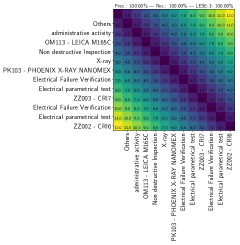
(a) LESE-3 cost matrix before flipping equipment. LESE-3 $=100.00\%$.

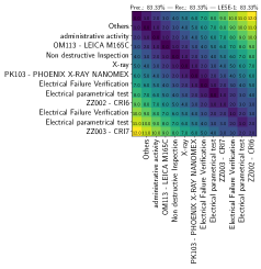
(b) LESE-1 cost matrix after flipping equipment. LESE-1 $=83.33\%$.

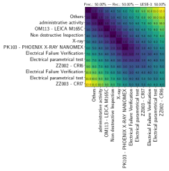
(c) LESE-3 cost matrix after flipping equipment. LESE-3 $=50.00\%$.

Figure 5: LESE-3 cost matrix before and after flipping equipment in triplet generated by GPT2. observe the final Levenshstein distance before flipping is $2$ and $6$ after flipping. The LESE-3 (F1-score) reflects this change in equipment and correlates with human evaluation.

LESE-1 and LESE-3 accurately measures the difference in this flip to a human level. Observe how the Levenshstein distance changes the heat on the images along the diagonal from index $9$ in Figure (5b) and index $7$ on Figure (5c). This changes indicate the time of occurrence of the $n$-gram Levenshstein deletion, insertion or substitution operations.

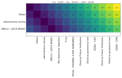
(a) LESE-3 cost matrix before transposing triplets. LESE-3 $=$ LESE-1 $=40.00\%$, Precision $=25.00\%$ & Recall $=100.00\%$.

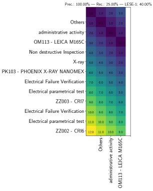
(b) LESE-3 cost matrix after transposing triplets. LESE-3 $=$ LESE-1 $=40.00\%$, Precision $=100.00\%$ & Recall $=25.00\%$.

Figure 6: LESE-3 cost matrix with unequal $3$-gram length of reference and hypothesis.

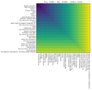
(a) LESE-3 cost matrix. LESE-3 $=40.00\%$, Precision $=25.00\%$ & Recall $=100.00\%$.

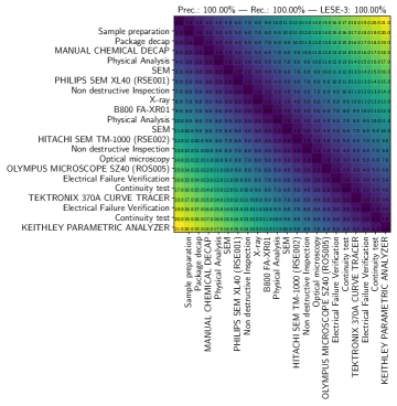
(b) LESE-3 cost matrix. LESE-3 $=40.00\%$, Precision $=100.00\%$ & Recall $=25.00\%$.

Figure 7: LESE-3 cost matrix with unequal $3$-gram length of reference and hypothesis.

When |r|${}_{\texttt{n-gram}}=1$ and less than |h|${}_{\texttt{n-gram}}$ or |h|${}_{\texttt{n-gram}}=1$ and less than |r|${}_{\texttt{n-gram}}$, the LESE-1 score is computed (See Figure (6)). A python implementation of the LESE-N algorithm is presented in the appendix. If we transpose Figure (6a) to (6b), the LESE-3 score is unchanged, however, precision becomes $100\%$ while recall is $25\%$. Other examples of LESE-3 evaluation are presented in Figures (7).

5 Conclusion

We evaluate the efficiency of pre-trained transformer models for the downstream task of failure analysis triplet generation. We observe that forward only auto-regressive modelling used in GPT2 and GPT3 gives it excellent capabilities to generate structured data. When adapted for FATG, GPT2 ROUGE scores outperforms other benchmarks for generating both short and long FATs, $\lambda$’s. Since, ROUGE, BLEU and METEOR scores do not accurately convey human-expert evaluation, we introduce Levenshstein Sequential Evaluation (LESE) metric. LESE-N performs on par with human expert judgment for different test cases. GPT2-Medium and Large models perform best on LESE-1 and LESE-3 triplet scores, which corresponds to human judgement.

Fine-tuned BART generates very short triplets and seeks contextual representation of triplets making it unfit for structured long-text sequences while GPT3, generates long story-telling-like data that do not necessarily follow known expert failure analysis FATs.

.1 Abbreviations

Abbreviation	Meaning
RCA	Root Cause Analysis
FMEA	Failure Mode and Effects Analysis
RE	Reliability Engineering
FA	Failure Analysis
FRACAS	Failure Reporting Analysis and Corrective Action System
FDR	Failure Description
FATs	Failure Analysis Triplets
FATG	Failure Analysis Triplet Generation
LM	Language Model
PLMs	Pre-trained Language Models
Seq2Seq	Sequence-to-Sequence
RNN	Recurrent Neural Network
LSTM	Long Short Term Memory
GRNN	Gated Recurrent Neural Network
PFFN	Position-wise Feed-Forward Network
PE	Position Embedding
BART	Bidirectional Auto-Regressive Transformer
GPT	Generative Pre-trained Transformers
BLEU	Bilingual Evaluation Understudy
ROUGE	Recall-Oriented Understudy for Gisting Evaluation
LESE	Levenshstein Sequential Evaluation
SS-FATG	Short sequence FATG
LS-FATG	Long sequence FATG

Table 9: A list of abbreviations and their respective meaning

.2 Python Implementation of LESE-N Algorithm.

⬇

import numpy as np

class LESE:

def __init__(self, a, b, n_gram):

’’’LESE: LEvenshstein Sequential Evaluation metric

Parameters

----------

a : str or list

Reference string sequence or list of string sequence.

b : str or list

Hypothesis string sequence or list of string sequence.

n_gram : int, optional

n-gram size. The default is 3. See lese(..) sub module

Returns

-------

None

’’’

self.a = a

self.b = b

self.n_gram = n_gram

self.lese(self.a, self.b, self.n_gram)

def precision_lev_(self, D_i_j, n_a, n_b, n):

max_n_a_n_b = max(n_a, n_b)

lev_seq = D_i_j//n

prec = max(0, abs((max_n_a_n_b - lev_seq))/n_b)

return prec

def recall_lev_(self, D_i_j, n_a, n_b, n):

max_n_a_n_b = max(n_a, n_b)

lev_seq = D_i_j//n

rec = max(0, abs((max_n_a_n_b - lev_seq))/n_a)

return rec

def f_score_lev_(self, D_i_j, n_a, n_b, n, beta = 1.):

’’’Sequential Levenshstein F1- score

Parameters

----------

D_i_j : float

Levenshstein distance.

n_a : int

N-gram length of reference sequence.

n_b : int

N-gram length of hypothesis sequence.

n : int

N-gram size.

beta : float, optional

beta weight for balancing precision-recall. The default is 1.

Returns

-------

float

Precision.

float

Recall.

float

f_score.

’’’

precision = self.precision_lev_(D_i_j, n_a, n_b, n)

recall = self.recall_lev_(D_i_j, n_a, n_b, n)

if precision == 0. and recall == 0.:

return 0., 0., 0.

else:

f_score = ((1+ np.square(beta))*precision*recall)/(np.square(beta)*precision+recall)

return precision, recall, f_score

def lese(self, a, b, n = 3):

’’’LESE: LEvenshstein Sequential Evaluation metric main module

Parameters

----------

a : str or list

Reference string sequence or list of string sequence.

b : str or list

Hypothesis string sequence or list of string sequence.

n : int, optional

n-gram size. The default is 3.

Returns

-------

Tuple

Tuple(Levenshstein distance, (precision, recall, f_1_score)).

Complexity

----------

Time: O(M*N)

Space: O(M*N)

’’’

if isinstance(a, str) and isinstance(b, str):

n_a = len(a)

n_b = len(b)

if(len(a)//n) ==1: n = 1

else: pass

if(len(b)//n) ==1: n = 1

else: pass

n_gram_a = len(a)//n #n-gram in reference

n_gram_b = len(b)//n #n-gram in hypothesis

if n_b == 0:

self.levenshstein_distance = n_a

self.precision_, self.recall_, self.f_score_ = (0.0, 0.0, 0.0)

return self.levenshstein_distance, self.precision_, self.recall_, self.f_score_

elif n_a == 0:

self.levenshstein_distance = n_b

self.precision_, self.recall_, self.f_score_ = (0.0, 0.0, 0.0)

return self.levenshstein_distance, self.precision_, self.recall_, self.f_score_

else:

pass

elif isinstance(a, list) and isinstance(b, list):

a = [x for x in a if x != ’nan’ if x != ’ ’ if x != ’’]

b = [x for x in b if x != ’nan’ if x != ’ ’ if x != ’’]

n_a = len(a)

n_b = len(b)

if(len(a)//n) ==1: n = 1

else: pass

if(len(b)//n) ==1: n = 1

else: pass

n_gram_a = len(a)//n

n_gram_b = len(b)//n

if n_b == 0:

self.levenshstein_distance = n_a

self.precision_, self.recall_, self.f_score_ = (0.0, 0.0, 0.0)

return self.levenshstein_distance, self.precision_, self.recall_, self.f_score_

elif n_a == 0:

self.levenshstein_distance = n_b

self.precision_, self.recall_, self.f_score_ = (0.0, 0.0, 0.0)

return self.levenshstein_distance, self.precision_, self.recall_, self.f_score_

else:

pass

self.D = np.zeros((n_a + 1, n_b + 1))

# Initialising first row using the length of string/list a: reference

for i in range(n_a + 1):

self.D[i][0] = i

# Initialising first column using the length of string/list b: hypothesis

for j in range(n_b + 1):

self.D[0][j] = j

#DP version

for i in range(1, n_a + 1):

for j in range(1, n_b + 1):

if a[i-1:i+n-1] == b[j-1:j+n-1]:

self.D[i][j] = self.D[i - 1][j - 1]

else:

insertion = 1 + self.D[i][j - 1] #insertion operation

deletion = 1 + self.D[i - 1][j] #deletion operation

substitution = 1 + self.D[i - 1][j - 1] #substitution operation

#select optimal cost, optimal cost == minimum cost of operation

self.D[i][j] = min(insertion, deletion, substitution)

self.levenshstein_distance = self.D[i][j]

self.precision_, self.recall_, self.f_score_ = self.f_score_lev_(self.D[i][j], n_gram_a, n_gram_b, n)

return self.levenshstein_distance, self.precision_, self.recall_, self.f_score_

Listing 1: Python Implementation of LESE-N Algorithm.

References

- Abidi et al., (2022) Abidi, M. H., Mohammed, M. K., and Alkhalefah, H. (2022). Predictive maintenance planning for industry 4.0 using machine learning for sustainable manufacturing. Sustainability (Switzerland), 14(6). Cited by: 0; All Open Access, Gold Open Access.
- ABS Group Inc. and Division, (1999) ABS Group Inc., R. and Division, R. (1999). Root Cause Analysis Handbook: A Guide to Effective Incident Investigation. G - Reference, Information and Interdisciplinary Subjects Series. Government Institutes.
- Ahmed et al., (2017) Ahmed, K., Keskar, N. S., and Socher, R. (2017). Weighted transformer network for machine translation.
- Bahdanau et al., (2014) Bahdanau, D., Cho, K., and Bengio, Y. (2014). Neural machine translation by jointly learning to align and translate.
- Bahdanau et al., (2015) Bahdanau, D., Cho, K., and Bengio, Y. (2015). Neural machine translation by jointly learning to align and translate. In Bengio, Y. and LeCun, Y., editors, 3rd International Conference on Learning Representations, ICLR 2015, San Diego, CA, USA, May 7-9, 2015, Conference Track Proceedings.
- Banerjee and Lavie, (2005) Banerjee, S. and Lavie, A. (2005). METEOR: An automatic metric for MT evaluation with improved correlation with human judgments. In Proceedings of the ACL Workshop on Intrinsic and Extrinsic Evaluation Measures for Machine Translation and/or Summarization, pages 65–72, Ann Arbor, Michigan. Association for Computational Linguistics.
- Bazu and Bajenescu, (2011) Bazu, M. and Bajenescu, T. T.-M. (2011). Failure analysis. A practical guide for manufacturers of electronic components and systems.
- Behbahani, (2006) Behbahani, A. R. (2006). Need for robust sensors for inherently fail-safe gas turbine engine controls, monitoring, and prognostics. volume 467, page 200 – 211. Cited by: 8.
- Brown et al., (2020) Brown, T., Mann, B., Ryder, N., Subbiah, M., Kaplan, J. D., Dhariwal, P., Neelakantan, A., Shyam, P., Sastry, G., Askell, A., Agarwal, S., Herbert-Voss, A., Krueger, G., Henighan, T., Child, R., Ramesh, A., Ziegler, D., Wu, J., Winter, C., Hesse, C., Chen, M., Sigler, E., Litwin, M., Gray, S., Chess, B., Clark, J., Berner, C., McCandlish, S., Radford, A., Sutskever, I., and Amodei, D. (2020). Language models are few-shot learners. In Larochelle, H., Ranzato, M., Hadsell, R., Balcan, M., and Lin, H., editors, Advances in Neural Information Processing Systems, volume 33, pages 1877–1901. Curran Associates, Inc.
- Chaturvedi et al., (2017) Chaturvedi, S., Peng, H., and Roth, D. (2017). Story comprehension for predicting what happens next. In Proceedings of the 2017 Conference on Empirical Methods in Natural Language Processing, pages 1603–1614, Copenhagen, Denmark. Association for Computational Linguistics.
- Chi et al., (2020) Chi, Z., Dong, L., Wei, F., Wang, W., Mao, X.-L., and Huang, H. (2020). Cross-lingual natural language generation via pre-training. In AAAI.
- Conneau et al., (2017) Conneau, A., Kiela, D., Schwenk, H., Barrault, L., and Bordes, A. (2017). Supervised learning of universal sentence representations from natural language inference data. In Palmer, M., Hwa, R., and Riedel, S., editors, Proceedings of the 2017 Conference on Empirical Methods in Natural Language Processing, EMNLP 2017, Copenhagen, Denmark, September 9-11, 2017, pages 670–680. Association for Computational Linguistics.
- Dai and Le, (2015) Dai, A. M. and Le, Q. V. (2015). Semi-supervised sequence learning. In Cortes, C., Lawrence, N., Lee, D., Sugiyama, M., and Garnett, R., editors, Advances in Neural Information Processing Systems, volume 28. Curran Associates, Inc.
- Devlin et al., (2019) Devlin, J., Chang, M., Lee, K., and Toutanova, K. (2019). BERT: pre-training of deep bidirectional transformers for language understanding. In Burstein, J., Doran, C., and Solorio, T., editors, Proceedings of the 2019 Conference of the North American Chapter of the Association for Computational Linguistics: Human Language Technologies, NAACL-HLT 2019, Minneapolis, MN, USA, June 2-7, 2019, Volume 1 (Long and Short Papers), pages 4171–4186. Association for Computational Linguistics.
- Ding et al., (2021) Ding, Z., Zhou, J., Liu, B., and Bai, W. (2021). Research of intelligent fault diagnosis based on machine learning. page 143 – 147. Cited by: 0.
- Duan, (2022) Duan, J. (2022). Improved systemic hazard analysis integrating with systems engineering approach for vehicle autonomous emergency braking system. ASCE-ASME Journal of Risk and Uncertainty in Engineering Systems, Part B: Mechanical Engineering, 8(3). Cited by: 0.
- Ezukwoke et al., (2021) Ezukwoke, K., Toubakh, H., Hoayek, A., Batton-Hubert, M., Boucher, X., and Gounet, P. (2021). Intelligent fault analysis decision flow in semiconductor industry 4.0 using natural language processing with deep clustering. In 2021 IEEE 17th International Conference on Automation Science and Engineering (CASE), pages 429–436.
- Gatt and Krahmer, (2018) Gatt, A. and Krahmer, E. (2018). Survey of the state of the art in natural language generation: Core tasks, applications and evaluation. J. Artif. Int. Res., 61(1):65–170.
- Gultekin et al., (2022) Gultekin, O., Cinar, E., Özkan, K., and Yazıcı, A. (2022). Real-time fault detection and condition monitoring for industrial autonomous transfer vehicles utilizing edge artificial intelligence. Sensors, 22(9). Cited by: 0; All Open Access, Gold Open Access, Green Open Access.
- (20) Holtzman, A., Buys, J., Du, L., Forbes, M., and Choi, Y. (2019a). The curious case of neural text degeneration.
- (21) Holtzman, A., Buys, J., Du, L., Forbes, M., and Choi, Y. (2019b). The curious case of neural text degeneration.
- Hu and Yang, (2019) Hu, B. and Yang, B. (2019). A particle swarm optimization algorithm for multi-row facility layout problem in semiconductor fabrication. Journal of Ambient Intelligence and Humanized Computing, 10(8):3201 – 3210. Cited by: 8.
- Huang et al., (2022) Huang, R., Li, J., Wang, Z., Xia, J., Chen, Z., and Li, W. (2022). Intelligent diagnostic and prognostic method based on multitask learning for industrial equipment. Zhongguo Kexue Jishu Kexue/Scientia Sinica Technologica, 52(1):123 – 137. Cited by: 0; All Open Access, Bronze Open Access.
- IFIP TC5 International Conference on Knowledge Enterprise: Intelligent Strategies in Product Design and Management, (2006) IFIP TC5 International Conference on Knowledge Enterprise: Intelligent Strategies in Product Design, M. and Management, P. (2006). IFIP Advances in Information and Communication Technology, 207:1 – 1041. Cited by: 0.
- Joshi et al., (2020) Joshi, M., Chen, D., Liu, Y., Weld, D. S., Zettlemoyer, L., and Levy, O. (2020). SpanBERT: Improving pre-training by representing and predicting spans. Transactions of the Association for Computational Linguistics, 8:64–77.
- Kim et al., (2017) Kim, Y., Denton, C., Hoang, L., and Rush, A. M. (2017). Structured attention networks.
- Kukich, (1983) Kukich, K. (1983). Design of a knowledge-based report generator. In Proceedings of the 21st Annual Meeting on Association for Computational Linguistics, ACL ’83, page 145–150, USA. Association for Computational Linguistics.
- Levenshtein, (1965) Levenshtein, V. I. (1965). Binary codes capable of correcting deletions, insertions, and reversals. Soviet physics. Doklady, 10:707–710.
- Lewis et al., (2019) Lewis, M., Liu, Y., Goyal, N., Ghazvininejad, M., Mohamed, A., Levy, O., Stoyanov, V., and Zettlemoyer, L. (2019). Bart: Denoising sequence-to-sequence pre-training for natural language generation, translation, and comprehension.
- Li et al., (2022) Li, H., Hu, G., Li, J., and Zhou, M. (2022). Intelligent fault diagnosis for large-scale rotating machines using binarized deep neural networks and random forests. IEEE Transactions on Automation Science and Engineering, 19(2):1109 – 1119. Cited by: 9.
- Li et al., (2021) Li, J., Tang, T., Zhao, W. X., and Wen, J.-R. (2021). Pretrained language models for text generation: A survey.
- Lin, (2004) Lin, C.-Y. (2004). ROUGE: A package for automatic evaluation of summaries. In Text Summarization Branches Out, pages 74–81, Barcelona, Spain. Association for Computational Linguistics.
- Lin and Hovy, (2003) Lin, C.-Y. and Hovy, E. (2003). Automatic evaluation of summaries using n-gram co-occurrence statistics. In Proceedings of the 2003 Conference of the North American Chapter of the Association for Computational Linguistics on Human Language Technology - Volume 1, NAACL ’03, page 71–78, USA. Association for Computational Linguistics.
- Lin et al., (2017) Lin, Z., Feng, M., Santos, C. N. d., Yu, M., Xiang, B., Zhou, B., and Bengio, Y. (2017). A structured self-attentive sentence embedding.
- Liu et al., (2016) Liu, P., Qiu, X., and Huang, X. (2016). Recurrent neural network for text classification with multi-task learning. In Proceedings of the Twenty-Fifth International Joint Conference on Artificial Intelligence, IJCAI’16, page 2873–2879. AAAI Press.
- Liu et al., (2018) Liu, P. J., Saleh, M., Pot, E., Goodrich, B., Sepassi, R., Kaiser, L., and Shazeer, N. (2018). Generating wikipedia by summarizing long sequences.
- Liu et al., (2020) Liu, Y., Gu, J., Goyal, N., Li, X., Edunov, S., Ghazvininejad, M., Lewis, M., and Zettlemoyer, L. (2020). Multilingual Denoising Pre-training for Neural Machine Translation. Transactions of the Association for Computational Linguistics, 8:726–742.
- (38) Liu, Y., Ott, M., Goyal, N., Du, J., Joshi, M., Chen, D., Levy, O., Lewis, M., Zettlemoyer, L., and Stoyanov, V. (2019a). Roberta: A robustly optimized bert pretraining approach.
- (39) Liu, Y., Ott, M., Goyal, N., Du, J., Joshi, M., Chen, D., Levy, O., Lewis, M., Zettlemoyer, L., and Stoyanov, V. (2019b). Roberta: A robustly optimized bert pretraining approach. ArXiv, abs/1907.11692.
- Mario, (1992) Mario, V. (1992). Failure reporting, analysis and corrective action system in the us semiconductor manufacturing equipment industry: A continuous improvement process. In Thirteenth IEEE/CHMT International Electronics Manufacturing Technology Symposium, pages 111–115.
- McCann et al., (2017) McCann, B., Bradbury, J., Xiong, C., and Socher, R. (2017). Learned in translation: Contextualized word vectors. In Proceedings of the 31st International Conference on Neural Information Processing Systems, NIPS’17, page 6297–6308, Red Hook, NY, USA. Curran Associates Inc.
- Melis et al., (2018) Melis, G., Dyer, C., and Blunsom, P. (2018). On the state of the art of evaluation in neural language models. In 6th International Conference on Learning Representations, ICLR 2018, Vancouver, BC, Canada, April 30 - May 3, 2018, Conference Track Proceedings. OpenReview.net.
- Merity et al., (2017) Merity, S., Keskar, N. S., and Socher, R. (2017). Regularizing and optimizing lstm language models.
- on Industry 4.0 and Smart Manufacturing, (2020) on Industry 4.0, I. C. and Smart Manufacturing, I. . (2020). volume 42. Cited by: 0.
- on Intelligent Computing and Science, (2011) on Intelligent Computing, I. C. and Science, I. (2011). Communications in Computer and Information Science, 134(PART 1). Cited by: 0.
- Pan and Yang, (2010) Pan, S. J. and Yang, Q. (2010). A survey on transfer learning. IEEE Transactions on Knowledge and Data Engineering, 22(10):1345–1359.
- Papineni et al., (2002) Papineni, K., Roukos, S., Ward, T., and Zhu, W.-J. (2002). Bleu: A method for automatic evaluation of machine translation. In Proceedings of the 40th Annual Meeting on Association for Computational Linguistics, ACL ’02, page 311–318, USA. Association for Computational Linguistics.
- Peters et al., (2018) Peters, M. E., Neumann, M., Iyyer, M., Gardner, M., Clark, C., Lee, K., and Zettlemoyer, L. (2018). Deep contextualized word representations.
- Phang et al., (2018) Phang, J., Févry, T., and Bowman, S. R. (2018). Sentence encoders on stilts: Supplementary training on intermediate labeled-data tasks. ArXiv, abs/1811.01088.
- Prajit Ramachandran, (2016) Prajit Ramachandran, Peter J. Liu, Q. V. L. (2016). Unsupervised pretraining for sequence to sequence learning. arXiv.
- Priyanka et al., (2022) Priyanka, E., Thangavel, S., Gao, X.-Z., and Sivakumar, N. (2022). Digital twin for oil pipeline risk estimation using prognostic and machine learning techniques. Journal of Industrial Information Integration, 26. Cited by: 9.
- Qiu et al., (2020) Qiu, X., Sun, T., Xu, Y., Shao, Y., Dai, N., and Huang, X. (2020). Pre-trained models for natural language processing: A survey. Science China Technological Sciences, 63(10):1872–1897.
- (53) Radford, A. and Narasimhan, K. (2018a). Improving language understanding by generative pre-training.
- (54) Radford, A. and Narasimhan, K. (2018b). Improving language understanding by generative pre-training.
- Radford et al., (2019) Radford, A., Wu, J., Child, R., Luan, D., Amodei, D., and Sutskever, I. (2019). Language models are unsupervised multitask learners.
- Raffel et al., (2020) Raffel, C., Shazeer, N., Roberts, A., Lee, K., Narang, S., Matena, M., Zhou, Y., Li, W., and Liu, P. J. (2020). Exploring the limits of transfer learning with a unified text-to-text transformer. Journal of Machine Learning Research, 21(140):1–67.
- Sai et al., (2022) Sai, A. B., Mohankumar, A. K., and Khapra, M. M. (2022). A survey of evaluation metrics used for nlg systems. ACM Comput. Surv., 55(2).
- Song et al., (2019) Song, K., Tan, X., Qin, T., Lu, J., and Liu, T.-Y. (2019). Mass: Masked sequence to sequence pre-training for language generation. In ICML.
- Vaswani et al., (2017) Vaswani, A., Shazeer, N., Parmar, N., Uszkoreit, J., Jones, L., Gomez, A. N., Kaiser, L., and Polosukhin, I. (2017). Attention is all you need. In Guyon, I., Luxburg, U. V., Bengio, S., Wallach, H., Fergus, R., Vishwanathan, S., and Garnett, R., editors, Advances in Neural Information Processing Systems, volume 30. Curran Associates, Inc.
- Wen et al., (2015) Wen, T.-H., Gasic, M., Mrksic, N., Su, P.-H., Vandyke, D., and Young, S. (2015). Semantically conditioned lstm-based natural language generation for spoken dialogue systems.
- Yang et al., (2019) Yang, Z., Dai, Z., Yang, Y., Carbonell, J., Salakhutdinov, R., and Le, Q. V. (2019). XLNet: Generalized Autoregressive Pretraining for Language Understanding. Curran Associates Inc., Red Hook, NY, USA.
- Zhang et al., (2019) Zhang, Y., Sun, S., Galley, M., Chen, Y.-C., Brockett, C., Gao, X., Gao, J., Liu, J., and Dolan, B. (2019). Dialogpt: Large-scale generative pre-training for conversational response generation.
- Zhu et al., (2015) Zhu, Y., Kiros, R., Zemel, R. S., Salakhutdinov, R., Urtasun, R., Torralba, A., and Fidler, S. (2015). Aligning books and movies: Towards story-like visual explanations by watching movies and reading books. 2015 IEEE International Conference on Computer Vision (ICCV), pages 19–27.