Strange Correlation Function for Average Symmetry-Protected Topological Phases

Abstract

We design a strange correlator for the recently discovered average symmetry-protected topological (ASPT) phases in $1d$ and $2d$. The strange correlator has long-range or power-law behavior if the density matrix $\rho$ is in a nontrivial ASPT phase. In all the $2d$ cases considered here, we find interesting connections between strange correlators and correlation functions in $2d$ loop models, based on which we can extract exact scaling exponents of the strange correlators.

I Introduction

Symmetry-protected topological (SPT) phases are short-range entanglement (SRE) quantum states which cannot be adiabatically connected to trivial product states in the presence of symmetries Gu and Wen (2009); Chen et al. (2011, 2012, 2013); Senthil (2015). SPT phases are natural generalizations of topological insulators and superconductors to strongly correlated fermionic and bosonic systems with internal and/or crystalline symmetries Lu and Vishwanath (2012); Wang and Gu (2020); Kapustin and Thorngren (2017); Cheng et al. (2018a); Levin and Gu (2012); Cheng et al. (2018b); Vishwanath and Senthil (2013); Wang and Senthil (2013); Wang et al. (2013); Fidkowski et al. (2013); Wang and Senthil (2014); Fu (2011); Hsieh et al. (2012); Isobe and Fu (2015); Song et al. (2017); Huang et al. (2017); Thorngren and Else (2018); Po et al. (2017); Cheng and Wang ; Zhang et al. (2020a, b); Tang et al. (2019); Zhang et al. (2022); Zhang (2022). Recently, it is shown that symmetry-protected short-range entanglement can still prevail even if part of the protecting symmetry is broken by quenched disorder locally but restored upon disorder averaging Ma and Wang (2022); Ringel et al. (2012); Mong et al. (2012); Fulga et al. (2014); Chou et al. (2018); Chou and Nandkishore (2021). This defines a new class of SPT phases dubbed average SPT (ASPT). (We will refer to ordinary SPT phases as clean SPTs in this paper.) The existence of ASPT, in addition to its theoretical novelties, provides practical applications as a symmetry-breaking disorder may be unavoidable in many settings, especially for crystalline SPT phases.

The nontrivial features of clean SPT phases often manifest on the physical boundaries which carry ’t Hooft anomalies of the symmetry, while the bulk correlation functions of local observables all decay exponentially due to the energy gap. Therefore, the bulk detection of an SPT state is nontrivial if only a wavefunction without a boundary is available. One useful tool is the strange correlator You et al. (2014); Wu et al. (2015); Vanhove et al. (2018); Zhou et al. (2022); Lepori et al. (2022); Scaffidi and Ringel (2016) defined for a given wavefunction $|\Psi\rangle$ as $C(r,r^{\prime})=\frac{\langle\Psi|O(r)O(r^{\prime})|\Psi_{0}\rangle}{\langle\Psi|\Psi_{0}\rangle}$, where $|\Psi_{0}\rangle$ is a symmetric trivial state serving as a reference state, and $O$’s are local observables in the system. It has been demonstrated that, given a nontrivial SPT wavefunction, the strange correlator is generically long-range or power-law correlated in the long-distance limit. One of the advantages of the strange correlator is that we can robustly diagnose nontrivial SPT phases without restricting to the boundaries, which is particularly useful for SPTs whose protecting symmetry is broken by the existence of boundaries.

The main result of this work is a generalization of the strange correlator which can detect nontrivial ASPTs in 1 and 2 spatial dimensions. We will first define the notion of ASPT and its strange correlator in Sec. II. Then we demonstrate the power of the strange correlator with several examples in $1d$ and $2d$ in Sec. III. In $1d$, we study the average cluster state with $\mathbb{Z}_{2}\times\mathbb{Z}_{2}^{A}$ symmetry (“A” denotes an average symmetry) and show its strange correlator is a non-zero constant at a long distance. In $2d$, we have three non-trivial examples with $\mathbb{Z}_{2}\times\mathbb{Z}_{2}\times\mathbb{Z}_{2}^{A}$, $\mathbb{Z}_{3}\times\mathbb{Z}_{3}^{A}$, and $\mathbb{Z}_{2}^{f}\times\mathbb{Z}_{2}^{A}$. These examples cover $2d$ bosonic ASPT with so-called $0d$-decoration and $1d$-decoration as well as $2d$ fermionic ASPT with $1d$-decoration. We show that there is a deep connection between the strange correlator and the so-called watermelon correlators in $O(n)$ loop models. In addition, the nature of the decorated domain wall states plays an important universal role in determining the resulting loop model that the strange correlation maps to. The mapping to the statistical models helps us gain analytical control of the calculation of strange correlators. In all of our examples, we can obtain exact scaling exponents for the strange correlators.

II Strange Correlator – Definition

Let us first make a few remarks on the definition of ASPTMa and Wang (2022). In the ASPT setting, we consider a statistical ensemble with an average symmetry $G$ and an exact symmetry $K$. Namely, we look at a density matrix of the following form,

$$\rho=\sum_{\mathcal{D}}p_{\mathcal{D}}|\Psi_{\mathcal{D}}\rangle\langle\Psi_{\mathcal{D}}|,$$ (1)

where $\mathcal{D}$ denotes configurations of symmetry defects of the symmetry group $G$ and $|\Psi_{\mathcal{D}}\rangle$ is $K$-symmetric SRE wavefunctions with the said defect configurations. The probability $p_{\mathcal{D}}$ is chosen such that the correlation of disorder for symmetry $G$ is short-ranged, namely

$$\langle\phi^{\dagger}_{G}(r)\phi_{G}(r^{\prime})\rangle_{\rho}=\sum_{\mathcal{D}}p_{\mathcal{D}}\langle\phi^{\dagger}_{G}(r)\phi_{G}(r^{\prime})\rangle_{\mathcal{D}}\sim e^{-|r-r^{\prime}|/\xi},$$ (2)

where $\phi$ is the order parameter for $G$ symmetry. This is equivalent to say the symmetry defects of $G$ proliferate in the ensemble. A nontrivial ASPT refers to cases where the SRE properties of the state cannot be removed adiabatically without breaking the exact symmetry $K$ and keeping the short-range nature of the $G$ disorder.

Typically, the decorated domain wall picture captures the nontrivial SRE in an ASPT. More precisely, for a nontrivial ASPT, in each state of the ensemble, an $n$-dimensional SPT ground state wavefunction of the $K$ symmetry is put on every $n$-dimensional symmetry defect of the $G$ symmetry, which we refer as $nd$-decoration in this paper. Note that the exact symmetry $K$ is always a normal subgroup of the full symmetry group. In another word, $K$ and $G$ fit into the following short exact sequence:

$$1\rightarrow K\rightarrow\mathcal{G}\rightarrow G\rightarrow 1.$$ (3)

For a trivial group extension, namely $\mathcal{G}=K\times G$, the corresponding ASPT phase has a clean limit Wang et al. (2021). In another word, one can purify the mixed state to an SPT wavefunction with exact $K\times G$ symmetry. However, if the group extension is nontrivial, one can show that a consistent purification procedure is not possible. We dubbed the corresponding ASPT phase as intrinsically ASPT phase Ma et al. (2022). We stress that the strange correlator defined below can detect nontrivial ASPT of both classes.

For ASPT phases, boundary detection sometimes is no longer convenient. Especially in the $0d$-decoration case, the boundary of ASPT does not host gapless mode but has spontaneous $K$ charge fluctuations according to the disorder configurations of $G$Ma and Wang (2022). Here we design a strange correlator that can detect the ASPT order in the bulk of the system. To that end, let us first construct a strange density matrix from the ASPT density matrix, which has the following explicit form

$$\rho_{s}=\sum\limits_{\mathcal{D}}p_{\mathcal{D}}|\Psi_{\mathcal{D}}\rangle\langle\Phi_{\mathcal{D}}|,$$ (4)

where we have used the same probability distribution as in $\rho$, $|\Psi_{\mathcal{D}}\rangle$ is the decorated domain wall wavefunction, and $|\Phi_{\mathcal{D}}\rangle$ is a reference trivial wavefunction with the same disorder configurations. The strange density matrix can be viewed as a super-operator acting on the ASPT density matrices $\rho$ and some reference trivial density matrix $\rho_{0}=\sum_{\mathcal{D}}p_{\mathcal{D}}|\Phi_{\mathcal{D}}\rangle\langle\Phi_{\mathcal{D}}|$. In terms of the strange density matrix, the strange correlator of some local operators $\phi(r)$ is defined as

$$C(r,r^{\prime})=\frac{\mathrm{Tr}\left(\rho_{s}\phi(r)\phi(r^{\prime})\right)}{\mathrm{Tr}\rho_{s}}.$$ (5)

In general, we will consider two types of operators, the operators that transform nontrivially under $G$ symmetry and the ones that transform under $K$ symmetry. In the following, we will show with examples that the strange correlator has long-ranged or power-law decay behavior in the long distance if $\rho$ is a nontrivial ASPT. In fact, if the ASPT to be detected has a clean limit, we show in the Appendix A that the strange correlator defined above can be mapped back to the ordinary strange correlator for a clean SPT wavefunction which is generically away from the fixed point wavefunction. However, such mapping is not possible for intrinsically ASPTs as they do not allow a clean limit.

III Strange correlator – Examples

III.1 Warm-up – $1d$ Averaged Cluster State

The first example is the $1d$ averaged cluster state Chen et al. (2014) protected by $\mathbb{Z}_{2}\times\mathbb{Z}_{2}^{A}$ symmetry, which is an example of $0d$-decoration in $1d$. Consider a spin-1/2 chain with $2N$ spins and periodic boundary conditions. The clean limit of the ASPT has a stabilizer Hamiltonian $H=-\sum_{j=1}^{2N}Z_{j-1}X_{j}Z_{j+1}$ where $X$ and $Z$ are Pauli matrices that are anti-commute. The two $\mathbb{Z}_{2}$ symmetries are defined on the odd and even sites, respectively, $\mathbb{Z}_{2}^{\mathrm{odd}}=\prod_{j\in\mathrm{odd}}X_{j},~{}~{}\mathbb{Z}_{2}^{\mathrm{even}}=\prod_{j\in\mathrm{even}}X_{j}$. Now we break the $\mathbb{Z}_{2}^{\mathrm{even}}$ to an average symmetry $\mathbb{Z}_{2}^{A}$ by random Zeeman fields $\{h_{2j}^{\mathcal{D}}=\pm 1\}$, which leads the 1d cluster state to a mixed ensemble labeled by $\{H_{\mathcal{D}},|\Psi_{\mathcal{D}}\rangle,p_{\mathcal{D}}\}$. $H_{\mathcal{D}}$ is the Hamiltonian for a specific domain wall realization of $\mathbb{Z}_{2}^{\mathrm{even}}$, $H_{\mathcal{D}}=-\sum_{j}Z_{2j}X_{2j+1}Z_{2j+2}+h_{2j}^{\mathcal{D}}Z_{2j}$. $|\Psi_{\mathcal{D}}\rangle$ is the corresponding ground state, which has the following explicit form

$$|\Psi_{\mathcal{D}}\rangle=\sum_{j=1}^{N}|Z_{2j}=h_{2j}\rangle\otimes|X_{2j+1}=h_{2j}h_{2j+2}\rangle$$ (6)

We pick $p_{\mathcal{D}}=1/2^{N}$ as the probability of each domain wall configuration - which corresponds to an infinite temperature ensemble of the even spins. We take the reference trivial wavefunctions with the following form

$$|\Phi_{\mathcal{D}}\rangle=\sum_{j=1}^{N}|Z_{2j}=h_{2j}\rangle\otimes|X_{2j+1}=1\rangle,$$ (7)

where there is no charge attached to the domain wall. With all the above ingredients, we can explicitly calculate the strange correlator of the $Z_{i}$ operator on the odd sites of the $1d$ averaged cluster state as

$$C_{ZZ}(i,j)=\frac{\mathrm{Tr}(\rho_{s}Z_{i}Z_{j})}{\mathrm{Tr}\rho_{s}}=1$$ (8)

which is a long-range correlation as we advertised. Note that the strange correlator detects the nontrivial ASPT state even though the boundary of this APST has no gapless modes.

III.2 $2d$ Bosonic ASPT with $\mathbb{Z}_{2}\times\mathbb{Z}_{2}\times\mathbb{Z}_{2}^{A}$ Symmetry

The second example is a $2d$ ASPT with $\mathbb{Z}_{2}\times\mathbb{Z}_{2}\times\mathbb{Z}_{2}^{A}$ symmetry. This is an example of an ASPT with $1d$-decoration in $2d$. The ASPT state can be achieved by decorating the domain wall of the average $G=\mathbb{Z}_{2}$ symmetry with a $1d$ cluster state protected by the exact symmetry $K=\mathbb{Z}_{2}\times\mathbb{Z}_{2}$ symmetry. We can picture the wavefunction in each disorder configuration as in Fig. 1. In particular, we consider Ising degrees of freedom on the sites of a triangular lattice. We put two spin-1/2 degrees of freedom on each link - we conveniently call them even and odd spins. The symmetry transformations are the same as in the cluster state. Whenever there is a domain wall piercing through the links, a cluster state wavefunction is put on the domain wall. Otherwise, the two spin-1/2 on the same link will be polarized to the $x$-direction locally.

Figure 1: Decorated domain wall state for $\mathbb{Z}_{2}\times\mathbb{Z}_{2}\times\mathbb{Z}_{2}^{A}$ symmetry. We have Ising spins on the triangular lattice denoted by the green dots. On each of the links, two spin-1/2 degrees of freedom are attached. On a domain wall, depicted by the solid red line on the dual honeycomb lattice, the corresponding spins form a cluster state. If there is no domain wall going through the link, the two spins are polarized to $|+\rangle$ states.

III.2.1 Mapping to a loop model

Let us first calculate the strange correlator of the $Z$ operators on the even spins, namely,

$$C_{K}(r,r^{\prime})=\frac{\mathrm{Tr}\left(\rho_{s}Z_{r}Z_{r^{\prime}}\right)}{\mathrm{Tr}\rho_{s}}=\frac{\sum_{\mathcal{D}}p_{\mathcal{D}}\langle\Psi_{\mathcal{D}}|Z_{r}Z_{r^{\prime}}|\Phi_{\mathcal{D}}\rangle}{\sum_{\mathcal{D}}p_{\mathcal{D}}\langle\Psi_{\mathcal{D}}|\Phi_{\mathcal{D}}\rangle}.$$ (9)

The subscript $K$ denotes that we consider operators that transform nontrivially under $K$. We dub this type of strange correlator as $K$-strange correlator. Let us first consider the denominator of Eq. (9). The sum over $\mathcal{D}$ is a sum over domain wall configurations of the Ising spins. Without loss of generality, let us assume the probability distribution $p_{\mathcal{D}}$ has the form of the Boltzmann weight of a classical Ising model, or equivalently $p_{\mathcal{D}}=2\prod_{l\in\mathcal{D}}x^{-l}$, where $x=\exp(-2\beta)$ is the domain wall tension and the factor of 2 comes from the fact that for the same domain wall configuration there are 2 Ising spin configurations related by the $\mathbb{Z}_{2}$ symmetry. Here, without causing any confusion, we use $l$ to label both the domain wall and the length of the domain wall. For the ensemble to be in a $\mathbb{Z}_{2}^{A}$ preserving phase, we need $x>x_{c}^{\mathrm{Ising}}=1/\sqrt{3}$ on a triangular lattice. In each configuration, we have a factor of a wavefunction overlap. It can be decomposed into the product of overlap between a cluster state and a trivial state on each domain wall,

$$\langle\Psi_{\mathcal{D}}|\Phi_{\mathcal{D}}\rangle=\prod_{l\in\mathcal{D}}\langle\psi_{\mathrm{cluster}}|\psi_{0}\rangle(l)=\prod_{l\in\mathcal{D}}2\times 2^{-l}.$$ (10)

Here the overlap is calculated using the fixed point wavefunction of the cluster state and trivial state, for details see Appendix C. Each overlap factor decays with the length of the system, which makes perfect sense. The decay rate in general is not universal. However, the factor of 2 in front of the exponential decay is universal - it is related to the quantum dimension of the boundary modes of the decorated $1d$ SPT. This factor is crucial in determining the behavior of strange correlators as we will explain later. Gathering everything, the denominator can be written as

$$\mathrm{Tr}(\rho_{s})=2\sum_{\mathcal{D}}\tilde{x}^{-L(\mathcal{D})}2^{n(\mathcal{D})},$$ (11)

where $L(\mathcal{D})$ is the total length of domain wall and $n(\mathcal{D})$ is the number of domain walls in configuration $\mathcal{D}$. $\tilde{x}$ is $x/2$, where 1/2 is the loop tension renormalization coming from the wavefunction overlaps. A keen reader may find the resemblance between Eq. (11) and the partition function of an $O(n)$ loop model with $n=2$.

Now we are ready to look at the numerator. The crucial observation is that the correlation function $\langle\Psi_{\mathcal{D}}|Z_{r}Z_{r^{\prime}}|\Phi_{\mathcal{D}}\rangle$ can only pick up a non-zero value if the two measured spins reside on the same domain wall. The non-zero value is precisely the strange correlator of the $1d$ cluster state times the factor of wavefunction overlaps. Therefore, the strange correlator, in the end, can be written as

$$C_{K}(r,r^{\prime})=\frac{\sum_{\mathcal{D}^{\prime}}\langle Z_{r}Z_{r^{\prime}}\rangle_{S}\tilde{x}^{-L(\mathcal{D}^{\prime})}2^{n(\mathcal{D}^{\prime})}}{\sum_{\mathcal{D}}\tilde{x}^{-L(\mathcal{D})}2^{n(\mathcal{D})}},$$ (12)

conditioned on that in every configurations of $\mathcal{D}^{\prime}$ there must be a domain wall connecting $r$ and $r^{\prime}$. The factor $\langle Z_{r}Z_{r^{\prime}}\rangle_{S}$ is a non-zero constant as the strange correlator of the $1d$ cluster state. This quantity essentially maps to a certain correlator, more specifically the 2-leg watermelon correlator, in the $O(2)$ loop model Duplantier (1989). For the loop tension $\tilde{x}>x_{c}^{n=2}=1/\sqrt{2}$, the loop model will be in the dense loop phases, where the loops behave critically. The strange correlator has the following power-law behavior:

$$C_{K}(r,r^{\prime})\sim\frac{1}{|r-r^{\prime}|^{2\Delta_{2}}},$$ (13)

where $\Delta_{2}$ is known as the 2-leg exponent. Its value in the $O(2)$ loop model is $\Delta_{2}=1/2$. For a brief review of the $O(n)$ loop model and its correlation function, see Appendix B.

A careful reader may notice that, if we start from the bare loop tension $x\in[1/\sqrt{3},1/\sqrt{2}]$, then the renormalized loop tension $\tilde{x}$ is not in the dense loop phase. In fact, loop tension in this regime will flow to 0 in the IR and the system prefers to have no loops. Therefore, the strange correlator defined in Eq. (9) decays exponentially with distance. However, this does not indicate that the strange correlator fails to detect the ASPT order because we also need to include the strange correlator associated with operators that transform nontrivially under $G$ symmetry. Let us consider the $G$-strange correlator,

$$C_{G}(r,r^{\prime})=\frac{\mathrm{Tr}\left(\rho_{s}\sigma_{r}\sigma_{r^{\prime}}\right)}{\mathrm{Tr}\rho_{s}},$$ (14)

where $\sigma$’s are the Ising spins on the sites of the triangular lattice. Note if we were to put in the original ASPT density matrix here to calculate the correlator, then it would be short-ranged as the definition of ASPT. However, it is no longer the case since we are dealing with the strange density matrix. The strange density matrix essentially changed the statistical model from an $n=1$ loop model (describing the Ising domain wall configurations) to $n=2$. This strange correlator is in fact measuring the probability of two points sitting in the same domain. In the dilute loop phase where loops are suppressed, this correlator is in fact long-ranged, namely a non-zero constant at long distance,

$$C_{G}(r,r^{\prime})\sim\text{const},\ \ \text{for}\ \ \tilde{x}<1/\sqrt{2}.$$ (15)

Therefore, strange correlators are either long-ranged or power-law decaying in the whole regime where ASPT is well defined, as shown in the schematic phase diagram in Fig. 2.

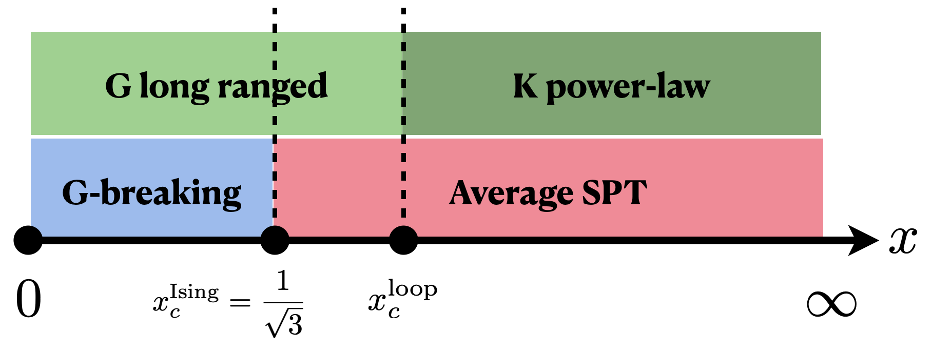
Figure 2: Phase diagram of the strange correlator. The ASPT is well defined in $x>x_{c}^{\text{Ising}}$. For $x<x_{c}^{\text{Ising}}$, the $G$ symmetry is spontaneously breaking in the ensemble. In the entire ASPT phase, the strange correlators are either long-ranged (in the $G$ symmetry sector) or quasi-long-ranged (in the $K$ symmetry sector).

III.2.2 Comment on the loop fugacity

We see that the mapping to the $O(2)$ loop model is critically dependent on the constant factor in Eq. (10). We would like to argue the universal nature of this factor by going away from the fixed point wavefunction using a field theoretical representation of the SPT wavefunction. It is known that the wavefunction of a 1d SPT state can be written as $O(3)$ non-linear sigma model (NL$\sigma$M) with a Wess–Zumino–Witten term at level-1. The overlap between an SPT wavefunction and a trivial state can be represented as,

$$\langle\Psi|\Phi\rangle=\int_{\mathcal{D}[\vec{n}(x)]}\exp\left(-\int_{x=0}^{L}\mathcal{L}[\vec{n}]+i\mathrm{WZW}_{1}[\vec{n}(x)]\right),$$ (16)

where $\mathcal{L}(n)$ contains the kinetic term of the NL$\sigma$M and possible anisotropic terms that break the $SO(3)$ symmetry. Doing a wick rotation, we can equivalently view this overlap as the thermal partition function at temperature $\beta=L$ of a quantum mechanical model of a charged particle moving on a sphere with a $2\pi$ magnetic monopole at the center. This Landau level problem has a robust 2-fold degeneracy of its ground state with energy $\frac{1}{2}\hbar\omega_{c}$ where $\omega_{c}$ depends on the details of the kinetic terms. The thermal partition function at large $\beta=L$ is given by $\langle\Psi|\Phi\rangle\cong 2\times e^{-L\hbar\omega_{c}/2}$, where the prefactor $2$ comes from the 2-fold ground state degeneracy. We also note that this overlap can be viewed as the boundary partition function of the SPT state. Therefore, the degeneracy is also the boundary degeneracy of the SPT that is decorated on the domain wall.

We can also provide a more rigorous argument based on the matrix product state (MPS) representation of $1d$ SPT phasesChen et al. (2011). A $K$-symmetric $1d$ SPT state can be described by an injective MPS,

$$|\Psi_{\mathrm{SPT}}\rangle=\sum\limits_{i_{1},\cdot\cdot\cdot i_{N}}\mathrm{Tr}\left[A_{i_{1}}\cdot\cdot\cdot A_{i_{N}}\right]|i_{1}\cdot\cdot\cdot i_{N}\rangle$$ (17)

which has the following symmetry property Chen et al. (2011)

$$\leavevmode\hbox to200.8pt{\vbox to57.54pt{\text{[drawing]}}}, V_{g} V_{g}^{\dagger} A_{j} A_{j} = U_{g} V_{g} V_{g}^{\dagger} A_{j} A_{j} = U_{g}$$ (18)

where $g\in K$, $U_{g}$, and $V_{g}$ are local unitary operators acting on the physical indices (dashed lines) and virtual indices (solid lines), respectively. For $g,h\in K$, the unitary operators $V_{g}$ and $V_{h}$ have the following property

$$V_{g}V_{h}=\omega(g,h)V_{gh},$$ (19)

where $\omega(g,h)\in\mathcal{H}^{2}[K,U(1)]$ which implies that $V_{g}$ is a projective representation of the group $G$.

Then we consider two MPSs of two topologically distinct $1d$ SPT phases $A$ and $B$, which are depicted by two 2-cocycles $\omega_{1}$ and $\omega_{2}$ in $\mathcal{H}^{2}[K,U(1)]$. Their overlap can be represented graphically as

(20)

where $E_{j}$ is the transfer matrix of two $1d$ MPSs. Furthermore, by acting $U_{g}$ and $U_{g}^{\dagger}$ to the physical indices of two MPSs, we have

(21)

i.e., $X_{g}E_{j}X_{g}^{\dagger}=E_{j}$, where $X_{g}=V_{g}^{\dagger}\otimes W_{g}$ that also satisfies the condition of projective representation of $K$ as

$$X_{g}X_{h}=\frac{\omega_{2}(g,h)}{\omega_{1}(g,h)}X_{gh}$$ (22)

Therefore, the transfer matrix $E_{j}$ has a $K$ symmetry and transforms projectively under $K$. For translation invariant MPSs, the overlap of these MPSs is $\mathrm{Tr}(E^{L})$ (where $L$ is the system size), which is determined by the largest eigenvalue of $E$.

For the $\mathbb{Z}_{2}$-classified $1d$ SPT phases, the largest eigenvalue of the transfer matrix will always have 2-fold degeneracy from the projectively imposed symmetry $G$, which leads to an overall factor $2$ of the wavefunction overlap of the trivial and nontrivial $1d$ SPT states.

Figure 3: $2d$ ASPT with $\mathbb{Z}_{2}^{f}\times\mathbb{Z}_{2}^{A}$ symmetry. There is one Ising spin on each site of the triangular lattice. Two Majorana modes are attached to each link. If a domain wall passes, the Majorana modes along the domain wall pair up in the same fashion as in the $1d$ Kitaev model. Otherwise, the 2 Majorana modes on a single link pair up locally with even fermion parity.

III.3 $2d$ Fermionic ASPT with $\mathbb{Z}_{2}^{f}\times\mathbb{Z}_{2}^{A}$ Symmetry

We can construct an example of fermionic ASPT which is analogous to the bosonic example above. In the fermionic case, we decorate the Ising domain walls with a Majorana chain with the anti-periodic boundary condition. More precisely, on each link of the triangular lattice, we put 2 Majorana modes, labeled $\chi_{A}$ and $\chi_{B}$, forming a complex fermion $c=(\chi_{A}+i\chi_{B})/2$. If an Ising domain wall goes through the link, the 2 Majorana modes will be paired with Majoranas from neighboring links. Otherwise, they pair up locally. For a demonstration, see Fig. 3.

Let us first consider the strange correlator of the complex fermion operators, namely

$$C_{K}(r,r^{\prime})=\frac{\mathrm{Tr}(\rho_{s}c(r)c(r^{\prime}))}{\mathrm{Tr}(\rho_{s})}.$$ (23)

For the Majorana chain decorationFidkowski and Kitaev (2011), the essential difference from the cluster state is the SPT-trivial overlap on the domain walls. Indeed, we can show for the fixed point wavefunction, the overlap has the following form (see Appendix C)

$$\langle\Psi_{\mathcal{D}}|\Phi_{\mathcal{D}}\rangle=\prod_{l\in\mathcal{D}}\langle\psi_{\mathrm{Majorana}}|\psi_{0}\rangle(l)=\prod_{l\in\mathcal{D}}\sqrt{2}\times\sqrt{2}^{-l}.$$ (24)

This means that the loop model now has loop fugacity $n=\sqrt{2}$. Similar to the previous case, on the numerator, the only configurations that can contribute to the strange correlator need to have one domain wall going through the two fermion positions. Therefore, the strange correlator reduces to

$$C_{K}(r,r^{\prime})=\frac{\sum_{\mathcal{D}^{\prime}}\langle c_{r}c_{r^{\prime}}\rangle_{S}\tilde{x}^{-L(\mathcal{D}^{\prime})}\sqrt{2}^{n(\mathcal{D}^{\prime})}}{\sum_{\mathcal{D}}\tilde{x}^{-L(\mathcal{D})}\sqrt{2}^{n(\mathcal{D})}},$$ (25)

where $\langle c_{r}c_{r^{\prime}}\rangle_{S}$=const as the strange correlator of the $1d$ Majorana chain. This strange correlator maps to the 2-leg watermelon correlator in the $O(n=\sqrt{2})$ model. The behavior of such a correlator depends on the value of $\tilde{x}=x/\sqrt{2}$. For $\tilde{x}>x_{c}^{n=\sqrt{2}}=1/\sqrt{2+\sqrt{2-\sqrt{2}}}\cong 0.601$, the loop model falls into the so-called dense loop fixed point, where the correlator has a similar power-law behavior as in Eq. (13) with an exponent $\Delta_{2}=1/3$. For $\tilde{x}=x_{c}^{n=\sqrt{2}}$, the loop model is at the dilute fixed point, where the exponent becomes $\Delta_{2}=3/5$. For $\tilde{x}<x_{c}^{n=\sqrt{2}}$, the loop model is no longer critical and the $K$-strange correlator becomes short-ranged.

In the regime $\tilde{x}<x_{c}^{n=\sqrt{2}}$ or $x<\sqrt{2}x_{c}^{n=\sqrt{2}}$, we can consider the $G$-strange correlator, which is defined as in Eq. (14). Since in this regime, the loop model is in a dilute loop phase, the $G$-strange correlator is again long-range ordered.

Figure 4: Top: the charge decoration rule for the $\mathbb{Z}_{3}\times\mathbb{Z}_{3}^{A}$ symmetry. A $2\pi/(-2\pi)$ vortex of $\mathbb{Z}_{3}^{A}$ is decorated with $+1/-1$ charge of the exact $\mathbb{Z}_{3}$ symmetry. The decoration rule is choosen in a rotational symmetric way. Bottom: The allowed configuration in the numerator of the strange correlator in Eq. 26. The allowed configuration must have a vortex and anti-vortex pair which is connected by three domain walls.

III.4 $2d$ Bosonic ASPT with $\mathbb{Z}_{3}\times\mathbb{Z}_{3}^{A}$ Symmetry

After discussing $2d$ cases with $1d$-decoration, let us consider a $2d$ example with $0d$-decoration structure. We construct a ASPT with $\mathbb{Z}_{3}\times\mathbb{Z}_{3}^{A}$. This ASPT has a structure that a nontrivial $\mathbb{Z}_{3}$ is attached on each vortex of the $\mathbb{Z}_{3}^{A}$ order parameter. The decoration rule is shown in Fig. 4. The mixed ensemble of quantum states consistent with this decoration defines a $\mathbb{Z}_{3}\times\mathbb{Z}_{3}^{A}$ ASPT.

We consider the strange correlation of creation and annihilation operators of $\mathbb{Z}_{3}$ charges, namely,

$$C_{K}(r,r^{\prime})=\frac{\mathrm{Tr}\left(\rho_{s}a^{\dagger}(r)a(r^{\prime})\right)}{\mathrm{Tr}\rho_{s}}.$$ (26)

Let us look at the denominator in this case, $\sum_{\mathcal{D}}p_{\mathcal{D}}\langle\Psi_{\mathcal{D}}|\Phi_{\mathcal{D}}\rangle$. We specify that the reference state has 0 charges decorated on the $\mathbb{Z}_{3}^{A}$ vortices. In this expression, the label $\mathcal{D}$ is supposed to represent all different configurations of $\mathbb{Z}_{3}^{A}$ order parameter. In particular, there will be domain wall and vortex configurations. However, if $\mathcal{D}$ has vortices, then the overlap function will be identically zero due to the nontrivial $\mathbb{Z}_{3}$ global charge decorated on the vortex in $|\Psi_{\mathcal{D}}\rangle$. Therefore, all the vortex configurations are killed in the summation and we end up again with a loop model. Note that there are two flavors of loops since there are two different kinds of domain walls in a $\mathbb{Z}_{3}$ model. Here, without loss of generality, we assume the probability distribution is given by a thermal weight of a $\mathbb{Z}_{3}$ clock model. As a result, the fugacities for the two kinds of domain walls are the same. The denominator can be written as

$$\mathrm{Tr}(\rho_{s})=3\sum_{\mathcal{D}^{\prime}}x^{-L(\mathcal{D^{\prime}})}2^{n(\mathcal{D^{\prime}})},$$ (27)

where $\mathcal{D}^{\prime}$ only contain loop configurations and the overall factor of $3$ comes from the $\mathbb{Z}_{3}$ symmetry. There is no loop tension renormalization from the wavefunction overlap. Eq. (27) again maps to the partition function of an $O(2)$ loop model.

By the same logic, the summation in the numerator of Eq. (26) should also contain only loop configurations except there should be a test vortex and a test anti-vortex right at position $r$ and $r^{\prime}$ respectively due to the charge creation and annihilation operators. We demonstrate examples of allowed configuration in Fig. 4. Therefore, the strange correlator maps to the 3-leg watermelon correlation of the $n=2$ loop model, namely

$$C_{K}(r,r^{\prime})\sim\frac{1}{|r-r^{\prime}|^{2\Delta_{3}}},$$ (28)

where $\Delta_{3}=9/8$ for $x>x_{c}^{{n=2}}=1/\sqrt{2}$.

Again, the same argument as before shows that, if the loop tension is $x<1/\sqrt{2}$, then the loop model is in the dilute loop phase and we can measure the analogous $G$-strange correlator to find long-range order.

IV Conclusion and Discussion

In this work, we define a way of detecting the nontrivial ASPT phases in the bulk by a strange correlator for the ASPT via a strange density matrix. For nontrivial ASPT, the corresponding strange correlator will show either long-range or power-law behavior and we present several examples to demonstrate the power of the strange correlator. In $2d$, all the strange correlation functions map to correlation functions in certain $2d$ loop models. Remarkably, the decorated SPT state on the symmetry defect of the average symmetry plays a peculiar role in determining the type of loop model and the dynamics of the loop model in the end. The nontrivial role of this decorated domain wall state in the strange correlator was noticed in Ref. Scaffidi and Ringel (2016) at a somewhat fine-tuned point of a clean SPT wavefunction. Our results apply to the ASPT case and also to clean SPT cases with more general SPT wavefunctions away from the fixed point. We also note that our construction of the strange correlator does not distinguish if the ASPT has a clean limit. For intrinsically ASPTs, the structure of the strange correlator and the mapping to the statistical models are essentially the same. Thus, we expect our strange correlator can detect intrinsically ASPT as well.

The generalization of the strange correlator to higher dimensional ASPTs is an exciting future direction. The map from the strange correlator to the statistical model is not limited to $2d$. For $3d$ ASPT with $1d$-decoration, the resulting statistical model will be $3d$ loop models for which many analytical results are also known. For $2d$-decoration, for example, a $3d$ ASPT phase with $K=\mathbb{Z}_{2}$ and $G=\mathbb{Z}_{2}^{A}$ from decorating a 2D Levin-Gu state on the codimension-1 $\mathbb{Z}_{2}^{A}$ domain wall, we imagine the strange correlator can be mapped to a correlation function in $3d$ membrane models. However, how exactly the nature of the decorated $2d$ state affects the resulting membrane model is not clear.

The intuition for the nontrivial behavior of the strange correlator for clean SPTs comes from a space-time rotation of the path integral representation of the strange correlator – the strange correlator is in some sense measuring the correlation function on the physical boundary of an SPT phase. Although it is not exact proof, such an argument provides much confidence in the nontriviality of strange correlator. In the ASPT case, the spatial disorder is strong. It is difficult to believe the wick rotation trick still holds. However, in all our examples, the strange correlators are still effective in detecting the ASPT order. To understand these in the future, we may need a deeper understanding of the underlying structure of strange correlators.

Appendix A Strange correlators of ASPT and clean SPT

In this section, we show that the strange correlator of ASPT phases is equivalent to the strange correlator of clean SPT phases assuming the ASPT phase has a clean limit.

As mentioned in the introduction, for clean SPT the strange correlator is defined as

$$C(r,r^{\prime})=\frac{\langle\Omega|\phi(r)\phi(r^{\prime})|\Psi\rangle}{\langle\Omega|\Psi\rangle}$$ (29)

where $\phi(r)$ is some local operator at the position $r$, $|\Psi\rangle$ is the wavefunction of the SPT phase, and $|\Omega\rangle$ is the wavefunction of a trivial product state.

Assuming the ASPT has a clean limit, we can always obtain a purified clean SPT wavefunction from the mixed density matrix that defines the ASPT state. In particular, we can have

$$\rho=\sum_{\mathcal{D}}p_{\mathcal{D}}|\Psi_{\mathcal{D}}\rangle\langle\Psi_{\mathcal{D}}|\longrightarrow|\Psi\rangle=\sum_{\mathcal{D}}\sqrt{p_{\mathcal{D}}}|\Psi_{\mathcal{D}}\rangle\otimes|\mathcal{D}\rangle,$$ (30)

where the state $|\mathcal{D}\rangle$ is just the quantum state corresponding to the configurations of disorder. For an ASPT with a clean limit, this procedure can always be done and the resulting wavefunction is guaranteed to be short-range entangled. However, if the ASPT does not have a clean limit, namely an intrinsically ASPT, such purification can be done, but the resulting wavefunction should not be short-range entangled. It is easy to come up with a trivial reference state

$$|\Omega\rangle=\sum_{\mathcal{D}}\sqrt{p_{\mathcal{D}}}|\Phi_{\mathcal{D}}\rangle|a_{\mathcal{D}}\rangle$$ (31)

where $|\Phi_{\mathcal{D}}\rangle$ are just decorating trivial product states on the domain walls.

On the one hand, the numerator of the strange correlator of ASPT phases (5) is

$$\mathrm{Tr}\left[{\rho_{S}}\phi(r)\phi(r^{\prime})\right]=\sum\limits_{\mathcal{D}}p_{\mathcal{D}}\langle\Phi_{\mathcal{D}}|\phi(r)\phi(r^{\prime})|\Psi_{\mathcal{D}}\rangle$$ (32)

On the other hand, the numerator of the strange correlator of the clean SPT phases (29) from the purified wavefunctions (31) is

$$\langle\Omega|\phi(r)\phi(r^{\prime})|\Psi\rangle=\sum\limits_{\mathcal{D}}p_{\mathcal{D}}\langle\Phi_{\mathcal{D}}|\phi(r)\phi(r^{\prime})|\Psi_{\mathcal{D}}\rangle$$ (33)

i.e., the numerators of the strange correlators (5) and (29) are identical. Following similar calculations, the denominators of (5) and (29) are also identical. Therefore, we conclude that if an ASPT phase has a clean limit, the strange correlator of this ASPT is identical to the strange correlator of the exact SPT phase in the clean limit, and they share the same long-range correlation properties.

Appendix B A review of $O(n)$ loop model and correlation function

In the main text, we have mapped the strange correlator of $2d$ ASPT phases to a certain correlation function in the self-avoiding $O(n)$ loop model on the honeycomb lattice. Here let us review some of the useful facts on the loop models. The partition function of the loop model is a sum over all possible self-avoiding loop configurations $\mathcal{C}$, weighted by a loop tension $x$ for the total length of loop configurations and a loop fugacity $n$ for the number of loops $|\mathcal{C}|$,

$$Z=\sum\limits_{\mathcal{C}}x^{\mathrm{length}}n^{|\mathcal{C}|}.$$ (34)

It is called the $O(n)$ loop model because the partition function of a honeycomb lattice of $O(n)$ spins can be transformed into the above form.

The phase diagram of the loop model is shown in Fig. 5. For a fixed value of $n\in[-2,2]$, there is a critical point $x_{c}=\left[2+\sqrt{2-n}\right]^{-1/2}$ which separates the so-called dense loop phase and dilute loop phase. For $x>x_{c}$/$x<x_{c}$, we call the corresponding phase the “dense/dilute” loop phase, and $x_{c}$ remarks their transition termed as the dilute fixed point Duplantier (1989).

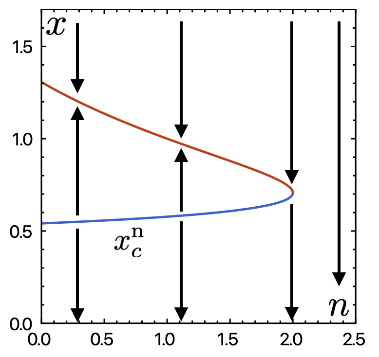
Figure 5: Phase diagram for loop models.

For the $O(n)$ loop model with $-2\leq n\leq 2$, the $L$-leg watermelon correlation function $C_{L}(\bm{x}-\bm{y})$ measures the probability that $L$ non-intersecting lines have a common source point $\bm{x}$ and shrink at the certain endpoint $\bm{y}$. At the dense phase $x>x_{c}$ and the dilute critical point $x_{c}$, the $L$-leg watermelon correlation function has power-law decay behavior as

$$C_{L}(\bm{x}-\bm{y})\sim|\bm{x}-\bm{y}|^{-2\Delta_{L}},$$ (35)

while $C_{L}(\bm{x}-\bm{y})$ decays exponentially in the dilute loop phase ($x<x_{c}$). The watermelon correlation is also power law right at the dilute fixed point but with a different exponent for $n<2$.

Let us the critical exponent $\Delta_{L}$. By the two-dimensional Coulomb gas technique Nienhuis (1987), the $O(n)$ model can be transformed into a solid-to-solid (SOS) model by orienting the loops in the continuum limit, which is a Gaussian model with the following action

$$S_{\mathrm{Gaussian}}=\frac{g}{4\pi}\int\mathrm{d}^{2}x(\nabla\phi)^{2},$$ (36)

where $g$ is the coupling constant of the Coulomb gas, such that

$$n=-2\cos(\pi g),$$ (37)

where $g\in[1,2]$ for the dilute critical point $x_{c}$ and $g\in[0,1]$ for the dense loop phase ($x>x_{c}$). The critical exponent $\Delta_{L}$ of the watermelon correlation function (35) is determined by

$$\Delta_{L}=\frac{g}{8}L^{2}-\frac{(1-g)^{2}}{2g},$$ (38)

for the $O(n)$ model where $n$ is parameterized by Eq. (37). In the main text, we have utilized Eq. (35) to calculate various critical exponents of watermelon correlation functions: $L=2$ and $L=3$ for $n=2$ model, and $L=2$ for $n=\sqrt{2}$ model.

Appendix C Wavefunction overlap of $1d$ dimerized topological states

In the main text, we emphasize that the wavefunction overlap of the decorated $1d$ SPT phase plays an essential role in the strange correlator (5). Therefore, in this section, we explicitly calculate the wavefunction overlap of $1d$ cluster states with trivial symmetric product states as well as the overlap of $1d$ Kitaev chain with trivial superconductor in systems with finite size using the fixed point wavefunctions.

For the $1d$ cluster state protected by $\mathbb{Z}_{2}\times\mathbb{Z}_{2}$, the wavefunction $|\psi\rangle$ of the $1d$ cluster state in $Z$-basis is explicitly written as

$$\langle\cdot\cdot\cdot s_{j-1}s_{j}s_{j+1}\cdot\cdot\cdot|\psi\rangle=(-1)^{\sum_{j}s_{j}s_{j+1}}/\sqrt{2^{2L}}$$ (39)

where $s_{j}=0,1$ and $2L$ is the number of qubits. Physically, there is a qubit with $X=-1$ at each domain wall of $Z$ (i.e., $Z_{j-1}Z_{j+1}=-1$) and a qubit with $X=1$ at the site away from the $Z$ domain wall. Then consider the trivial state $|\psi_{0}\rangle$ as the ground state of the disentangled Hamiltonian $H_{0}=-\sum_{j}X_{j}$, with the following explicit form

$$|\psi_{0}\rangle=\bigotimes\limits_{j=1}^{2L}\frac{1}{\sqrt{2}}(|\uparrow\rangle+|\downarrow\rangle)_{j}=\bigotimes\limits_{j=1}^{2L}|X_{j}=1\rangle$$ (40)

Hence the overlap of $1d$ cluster state (39) and trivial product state (40) is

$$\langle\psi_{0}|\psi\rangle=\frac{1}{2^{L-1}}=2\times 2^{-L}$$ (41)

As we have emphasized in the main text, the prefactor 2 is related to the quantum dimension of the boundary of the $1d$ SPT state.

Next, we consider the Majorana chain, with the following Hamiltonian

$$H=-\sum\limits_{j}c_{j}^{\dagger}c_{j+1}+h.c.-\sum\limits_{j}c_{j}c_{j+1}+h.c.$$ (42)

The ground states wavefunctions of the Majorana chain are

$$\begin{aligned} &|\Psi_{0}^{\mathrm{even}}\rangle=\frac{1}{\sqrt{2}}\left(|\Psi_{0}^{+}\rangle+|\Psi_{0}^{-}\rangle\right)\\ &|\Psi_{0}^{\mathrm{odd}}\rangle=\frac{1}{\sqrt{2}}\left(|\Psi_{0}^{+}\rangle-|\Psi_{0}^{-}\rangle\right)\end{aligned}$$ (43)

where the superscript even/odd represents the even/odd fermion parity of the ground state wavefunctions, and

$$|\Psi_{0}^{\pm}\rangle=\frac{1}{2^{L/2}}e^{\pm c_{1}^{\dagger}}e^{\pm c_{2}^{\dagger}}\cdot\cdot\cdot e^{\pm c_{L}^{\dagger}}|0\rangle$$ (44)

It is well-known that the ground state of the Majorana chain with periodic/anti-periodic boundary condition (PBC/anti-PBC) has odd/even fermion parity, hence $|\Psi_{0}^{\mathrm{even}}$/$|\Psi_{0}^{\mathrm{odd}}\rangle$ is the ground state wavefunction of the Majorana chain with anti-PBC/PBC. Then consider the atomic insulator as the $1d$ trivial product state, with the following disentangled Hamiltonian

$$H_{0}=\mu\sum\limits_{j}c_{j}^{\dagger}c_{j},~{}\mu>0$$ (45)

whose ground state wavefunction is the unoccupied vacuum state $|0\rangle$, with even fermion parity. Hence the wavefunction overlap between $|0\rangle$ and $|\Psi_{0}^{\mathrm{odd}}$ vanishes because of the different fermion parity, and the wavefunction overlap between $|0\rangle$ and $|\Psi_{0}^{\mathrm{even}}\rangle$ is

$$\langle 0|\Psi_{0}^{\mathrm{even}}\rangle=\left(\frac{1}{\sqrt{2}}\right)^{L-1}=\sqrt{2}\times 2^{-L/2},$$ (46)

where the prefactor $\sqrt{2}$ also coincides with the quantum dimension of the boundary Majorana zero modes of the $1d$ Majorana chain.

References

- Gu and Wen (2009) Z.-C. Gu and X.-G. Wen, “Tensor-entanglement-filtering renormalization approach and symmetry-protected topological order,” Phys. Rev. B 80, 155131 (2009).
- Chen et al. (2011) X. Chen, Z.-C. Gu, and X.-G. Wen, “Classification of gapped symmetric phases in one-dimensional spin systems,” Phys. Rev. B 83, 035107 (2011).
- Chen et al. (2012) X. Chen, Z.-C. Gu, Z.-X. Liu, and X.-G. Wen, “Symmetry-protected topological orders in interacting bosonic systems,” Science 338, 1604–1606 (2012).
- Chen et al. (2013) X. Chen, Z.-C. Gu, Z.-X. Liu, and X.-G. Wen, “Symmetry protected topological orders and the group cohomology of their symmetry group,” Phys. Rev. B 87, 155114 (2013).
- Senthil (2015) T. Senthil, “Symmetry-protected topological phases of quantum matter,” Annu. Rev. Condens. Matter Phys. 6, 299–324 (2015).
- Lu and Vishwanath (2012) Yuan-Ming Lu and Ashvin Vishwanath, “Theory and classification of interacting integer topological phases in two dimensions: A chern-simons approach,” Phys. Rev. B 86, 125119 (2012).
- Wang and Gu (2020) Q.-R. Wang and Z.-C. Gu, “Construction and classification of symmetry-protected topological phases in interacting fermion systems,” Phys. Rev. X 10, 031055 (2020), arXiv:1811.00536 [cond-mat.str-el] .
- Kapustin and Thorngren (2017) Anton Kapustin and Ryan Thorngren, “Fermionic spt phases in higher dimensions and bosonization,” Journal of High Energy Physics 2017, 80 (2017).
- Cheng et al. (2018a) M. Cheng, Z. Bi, Y.-Z. You, and Z.-C. Gu, “Classification of symmetry-protected phases for interacting fermions in two dimensions,” Phys. Rev. B 97, 205109 (2018a).
- Levin and Gu (2012) M. Levin and Z.-C. Gu, “Braiding statistics approach to symmetry-protected topological phases,” Phys. Rev. B 86, 115109 (2012).
- Cheng et al. (2018b) M. Cheng, N. Tantivasadakarn, and C. Wang, “Loop braiding statistics and interacting fermionic symmetry-protected topological phases in three dimensions,” Phys. Rev. X 8, 011054 (2018b).
- Vishwanath and Senthil (2013) A. Vishwanath and T. Senthil, “Physics of three-dimensional bosonic topological insulators: Surface-deconfined criticality and quantized magnetoelectric effect,” Phys. Rev. X 3, 011016 (2013).
- Wang and Senthil (2013) C. Wang and T. Senthil, “Boson topological insulators: A window into highly entangled quantum phases,” Phys. Rev. B 87, 235122 (2013).
- Wang et al. (2013) C. Wang, A. C. Potter, and T. Senthil, “Gapped symmetry preserving surface state for the electron topological insulator,” Phys. Rev. B 88, 115137 (2013).
- Fidkowski et al. (2013) L. Fidkowski, X. Chen, and A. Vishwanath, “Non-abelian topological order on the surface of a 3d topological superconductor from an exactly solved model,” Phys. Rev. X 3, 041016 (2013).
- Wang and Senthil (2014) C. Wang and T. Senthil, “Interacting fermionic topological insulators/superconductors in three dimensions,” Phys. Rev. B 89, 195124 (2014).
- Fu (2011) L. Fu, “Topological crystalline insulators,” Phys. Rev. Lett. 106, 106802 (2011).
- Hsieh et al. (2012) T. H. Hsieh, H. Lin, J. Liu, W. Duan, A. Bansil, and L. Fu, “Topological crystalline insulators in the snte material class,” Nat. Commun. 3, 982 (2012).
- Isobe and Fu (2015) H. Isobe and L. Fu, “Theory of interacting topological crystalline insulators,” Phys. Rev. B 92, 081304(R) (2015).
- Song et al. (2017) H. Song, S.-J. Huang, L. Fu, and M. Hermele, “Topological phases protected by point group symmetry,” Phys. Rev. X 7, 011020 (2017).
- Huang et al. (2017) S.-J. Huang, H. Song, Y.-P. Huang, and M. Hermele, “Building crystalline topological phases from lower-dimensional states,” Phys. Rev. B 96, 205106 (2017).
- Thorngren and Else (2018) Ryan Thorngren and Dominic V. Else, “Gauging spatial symmetries and the classification of topological crystalline phases,” Phys. Rev. X 8, 011040 (2018).
- Po et al. (2017) H. C. Po, A. Vishwanath, and H. Watanabe, “Symmetry-based indicators of band topology in the 230 space groups,” Nature Communications 8, 50 (2017).
- (24) M. Cheng and C. Wang, “Rotation symmetry-protected topological phases of fermions,” arXiv:1810.12308 [cond-mat.str-el] .
- Zhang et al. (2020a) J.-H. Zhang, Q.-R. Wang, S. Yang, Y. Qi, and Z.-C. Gu, “Construction and classification of point-group symmetry-protected topological phases in two-dimensional interacting fermionic systems,” Phys. Rev. B 101, 100501(R) (2020a).
- Zhang et al. (2020b) J.-H. Zhang, S. Yang, Y. Qi, and Z.-C. Gu, “Real-space construction of crystalline topological superconductors and insulators in 2d interacting fermionic systems,” Phys. Rev. Research 4, 033081 (2022) (2020b), 10.1103/PhysRevResearch.4.033081, arXiv:2012.15657 [cond-mat.str-el] .
- Tang et al. (2019) F. Tang, H. C. Po, A. Vishwanath, and X. Wan, “Comprehensive search for topological materials using symmetry indicators,” Nature 566, 486 (2019).
- Zhang et al. (2022) Jian-Hao Zhang, Yang Qi, and Zheng-Cheng Gu, “Construction and classification of crystalline topological superconductor and insulators in three-dimensional interacting fermion systems,” (2022), arXiv:2204.13558 [cond-mat.str-el] .
- Zhang (2022) Jian-Hao Zhang, “Strongly correlated crystalline higher-order topological phases in two-dimensional systems: A coupled-wire study,” Physical Review B 106, l020503 (2022).
- Ma and Wang (2022) Ruochen Ma and Chong Wang, “Average symmetry-protected topological phases,” (2022), arXiv:2209.02723 [cond-mat.str-el] .
- Ringel et al. (2012) Zohar Ringel, Yaacov E. Kraus, and Ady Stern, “Strong side of weak topological insulators,” Physical Review B 86, 045102 (2012).
- Mong et al. (2012) Roger S. K. Mong, Jens H. Bardarson, and Joel E. Moore, “Quantum transport and two-parameter scaling at the surface of a weak topological insulator,” Physical Review Letters 108, 076804 (2012).
- Fulga et al. (2014) I. C. Fulga, B. van Heck, J. M. Edge, and A. R. Akhmerov, “Statistical topological insulators,” Physical Review B 89, 155424 (2014).
- Chou et al. (2018) Yang-Zhi Chou, Rahul M. Nandkishore, and Leo Radzihovsky, “Gapless insulating edges of dirty interacting topological insulators,” Physical Review B 98, 054205 (2018).
- Chou and Nandkishore (2021) Yang-Zhi Chou and Rahul M. Nandkishore, “Marginally localized edges of time-reversal symmetric topological superconductors,” Physical Review B 103, 075120 (2021).
- You et al. (2014) Yi-Zhuang You, Zhen Bi, Alex Rasmussen, Kevin Slagle, and Cenke Xu, “Wave function and strange correlator of short-range entangled states,” Physical Review Letters 112, 247202 (2014).
- Wu et al. (2015) Han-Qing Wu, Yuan-Yao He, Yi-Zhuang You, Cenke Xu, Zi Yang Meng, and Zhong-Yi Lu, “Quantum monte carlo study of strange correlator in interacting topological insulators,” Physical Review B 92, 165123 (2015).
- Vanhove et al. (2018) Robijn Vanhove, Matthias Bal, Dominic J. Williamson, Nick Bultinck, Jutho Haegeman, and Frank Verstraete, “Mapping topological to conformal field theories through strange correlators,” Physical Review Letters 121, 177203 (2018).
- Zhou et al. (2022) Chengkang Zhou, Meng-Yuan Li, Zheng Yan, Peng Ye, and Zi Yang Meng, “Detecting subsystem symmetry protected topological order through strange correlators,” (2022), arXiv:2209.12917 [cond-mat.str-el] .
- Lepori et al. (2022) Luca Lepori, Michele Burrello, Andrea Trombettoni, and Simone Paganelli, “Strange correlators for topological quantum systems from bulk-boundary correspondence,” (2022), arXiv:2209.04283 [cond-mat.str-el] .
- Scaffidi and Ringel (2016) Thomas Scaffidi and Zohar Ringel, “Wave functions of symmetry-protected topological phases from conformal field theories,” Physical Review B 93, 115105 (2016).
- Wang et al. (2021) Qing-Rui Wang, Shang-Qiang Ning, and Meng Cheng, “Domain wall decorations, anomalies and spectral sequences in bosonic topological phases,” (2021), arXiv:2104.13233 [cond-mat.str-el] .
- Ma et al. (2022) Ruochen Ma, Jian-Hao Zhang, Zhen Bi, Meng Cheng, and Chong Wang, “Intrinsically average symmetry-protected topological phases,” to appear (2022).
- Chen et al. (2014) Xie Chen, Yuan-Ming Lu, and Ashvin Vishwanath, “Symmetry-protected topological phases from decorated domain walls,” Nature Communications 5 (2014), 10.1038/ncomms4507.
- Duplantier (1989) Bertrand Duplantier, “Two-dimensional fractal geometry, critical phenomena and conformal invariance,” Physics Reports 184, 229–257 (1989).
- Fidkowski and Kitaev (2011) L. Fidkowski and A. Kitaev, Phys. Rev. B 83, 075103 (2011).
- Lee et al. (2022) Jong Yeon Lee, Yi-Zhuang You, and Cenke Xu, “Symmetry protected topological phases under decoherence,” To appear (2022).
- Nienhuis (1987) B. Nienhuis, Phase Transitions and Critical Phenomena, edited by C. Domb and J. L. Lebowitz (Academic, London, 1987).