Uncertainty quantification for random domains
using periodic random variables
Abstract
We consider uncertainty quantification for the Poisson problem subject to domain uncertainty. For the stochastic parameterization of the random domain, we use the model recently introduced by Kaarnioja, Kuo, and Sloan (SIAM J. Numer. Anal., 2020) in which a countably infinite number of independent random variables enter the random field as periodic functions. We develop lattice quasi-Monte Carlo (QMC) cubature rules for computing the expected value of the solution to the Poisson problem subject to domain uncertainty. These QMC rules can be shown to exhibit higher order cubature convergence rates permitted by the periodic setting independently of the stochastic dimension of the problem. In addition, we present a complete error analysis for the problem by taking into account the approximation errors incurred by truncating the input random field to a finite number of terms and discretizing the spatial domain using finite elements. The paper concludes with numerical experiments demonstrating the theoretical error estimates.
1 Introduction
Modeling domain uncertainty is pertinent in many engineering applications, where the shape of the object may not be perfectly known. For example, one might think of manufacturing imperfections in the shape of products fabricated by line production, or shapes which stem from inverse problems such as tomography.
If the domain perturbations are small, one can apply the perturbation technique as in, e.g., [2, 13, 17]. In that approach, which is based on Eulerian coordinates, the shape derivative is used to linearize the problem under consideration around a nominal reference geometry. By Hadamard’s theorem, the resulting linearized equations for the first order shape sensitivities are homogeneous equations posed on the nominal geometry, with inhomogeneous boundary data only. By using a first order shape Taylor expansion, one can derive tensor deterministic partial differential equations (PDEs) for the statistical moments of the problem.
The approach we consider in this work is the domain mapping approach. It transfers the shape uncertainty onto a fixed reference domain and hence reflects the Lagrangian setting. Especially, it allows us to deal with large deformations, see [27, 31] for example. Analytic dependency of the solution on the random domain mapping in the case of the Poisson equation was shown in [3, 15] and in the case of linear elasticity in [14]. Related shape holomorphy for acoustic and electromagnetic scattering problems has been shown in [19, 21] and for Stokes and Navier-Stokes equations in [4]. Mixed spatial and stochastic regularity of the solutions to the Poisson equation on random domains, required for multilevel cubature methods, has been recently proved in [16].
In order to introduce the domain mapping approach, let be a probability space, where is the set of possible outcomes, the -algebra is the set of all events, and is a probability measure. We are interested in uncertainty quantification for the Poisson problem
| (1.1) |
where the domain , , is assumed to be uncertain. In the domain mapping framework, one starts with a reference domain . For example, in a manufacturing application, might be the planned domain provided by computer-aided design with no imperfections. It is assumed that a random perturbation field
is prescribed. The Poisson problem (1.1) on the perturbed domain is then transformed onto the fixed reference domain by a change of variable. This results in a PDE on the reference domain, equipped with a random coefficient and a random source term, which are correlated by the random deformation, and complicated by the occurrence of the Jacobian of the transformation. Note that the dependence on the random perturbation field is nonlinear. Nonetheless, in the domain mapping approach, the reference domain needs only to be Lipschitz, while the random perturbations have to be -smooth. This is in contrast to the perturbation approach mentioned above, where both the reference domain and the random perturbations need to be -smooth.
The approach adopted in this paper is first to truncate the initially infinite number of scalar random variables to a finite (but possibly large) number; then to approximate the transformed and truncated PDE on the reference domain by a finite element method; and finally to approximate the expected value of the solution (which is an integral, possibly high dimensional) by a carefully designed quasi-Monte Carlo (QMC) method—i.e., an equal weight cubature rule.
In [3, 15], the perturbation field was represented by an affine, vector-valued Karhunen–Loève expansion, under the assumption of uniformly independent and identically distributed random variables. In this work, we instead expand the perturbation field using periodic random variables, following the recent work [23]. The advantage of the periodic setting is that it permits higher order convergence of the QMC approximation to the expectation of the solution to (1.1). The periodic representation is equivalent in law to an affine representation of the input random field, where the random variables entering the series are i.i.d. with the Chebyshev probability density , . The density is associated with Chebyshev polynomials of the first kind, which is a popular family of basis functions in the method of generalized polynomial chaos (gPC). The choice of density is a modeling assumption, and it might be argued that in many applications choosing the Chebyshev density over the uniform density is a matter of taste rather than conviction, see [22, Sections 1–2] for more discussion.
The paper is organized as follows. The problem is formulated in Section 2, after which Section 3 establishes the regularity of the solution with respect to the stochastic variables; a more difficult task than in most such applications because of the nonlinear nature of the transformation, but a prerequisite for the design of good QMC rules. Section 4 considers error analysis, estimating separately the errors from dimension truncation, finite element approximation and QMC cubature. In the latter case, the error analysis leads to the design of appropriate weight parameters for the function space, ones that allow rigorous error bounds for the QMC contribution to the error. Numerical experiments that test the theoretical analysis are presented in Section 5, and some conclusions are drawn in Section 6. The appendix A contains several technical results required for the parametric regularity analysis.
2 Problem formulation
2.1 Notations
Let denote a set of parameters. Let us fix a bounded domain with Lipschitz boundary and as the reference domain.
We use multi-index notation throughout this paper. The set of all finitely supported multi-indices is denoted by , where is the support of a multi-index . For any sequence of real numbers and any , we define
where the product over the empty set is defined as by convention. We also define the multi-index notation
for higher order partial derivatives with respect to variable .
For any matrix , let denote the set of all singular values of and let denote the matrix spectral norm. For a function on we define
where we apply the vector 2-norm (Euclidean norm) or matrix 2-norm (spectral norm) depending on whether is a vector or a matrix. Similarly, we define
where is the gradient vector if is a scalar, and is the Jacobian matrix if is a vector. We will also need the standard Sobolev norm
for a scalar function in . We also define the norm
where is a nonempty domain.
In this paper we will make use of Stirling numbers of the second kind defined by
for integers , except for .
2.2 Parameterization of domain uncertainty
Let be a vector field such that
| (2.1) |
with stochastic fluctuations . Denoting the Jacobian matrix of by , the Jacobian matrix of vector field is
We assume that the family of admissible domains is parameterized by
and define the hold-all domain by setting
The convention of explicitly writing down the factor in (2.1) is not a crucial part of the analysis, but it ensures that the mean and covariance of the vector field match those of an affine and uniform parameterization for representing domain uncertainty using the same sequence of stochastic fluctuations , with the uniform random variables supported on . See also the discussion in [23].
In order to ensure that the aforementioned domain parameterization is well-posed and to enable our subsequent analysis of dimension truncation and finite element errors, we state the following assumptions for later use:
-
(A1)
For each , is an invertible, twice continuously differentiable vector field.
-
(A2)
For some , there holds
for all .
-
(A3)
There exist constants such that
where denotes the set of all singular values of the Jacobian matrix.
-
(A4)
There holds for all , and
-
(A5)
For some , there holds
-
(A6)
.
-
(A7)
The reference domain is a convex, bounded polyhedron.
For later convenience we define the sequence and constant by setting
| (2.2) |
It follows that we can take .
Remark. Under assumption (A3), there holds
| (2.3) |
This follows from the continuity of the determinant and .
2.3 The variational formulation on the reference domain
The variational formulation of the model problem (1.1) can be stated as follows: for , find such that
| (2.4) |
where is assumed to be an analytic function.
We can transport the variational formulation (2.4) to the reference domain by a change of variable. Let us first define the matrix-valued function
| (2.5) |
the transport coefficient
| (2.6) |
and the transported source term
Then we can recast the problem (2.4) on the reference domain as follows: for , find such that
| (2.7) |
for all .
3 Parametric regularity of the solution
In order to develop higher order rank-1 lattice cubature rules for the purpose of integrating the solution of (2.7) with respect to the parametric variable, we need to derive bounds on the partial derivatives in the Sobolev norm .
The analysis presented in this section is based on [15] and proceeds as follows:
- •
- •
- •
-
•
Finally, the main result of this section is stated in Theorem 3.7 which contains the partial derivative bound for , , making use of the aforementioned results.
3.1 Parametric regularity of the transport coefficient
Lemma 3.1.
Proof.
We will first derive a regularity bound for , . The bound for follows by applying implicit differentiation to the identity .
From the definition of it is easy to see that for any multi-index and any and we have
| (3.2) |
Taking the matrix -norm, we obtain
and hence with (2.2) we obtain
| (3.3) |
Now the Leibniz product rule yields for ,
and after taking the matrix 2-norm on both sides and then the -norm over we obtain
The bounds in (3.3) indicate that only the derivatives with will survive. Indeed, for with , only for remain, while for with and , only and remain. On the other hand, for with , in each term at least one of the factors must vanish. We conclude that
| (3.4) |
where we used for all .
Our assumption (A3) immediately yields for all that
which proves the lemma for the case . Now we consider . To obtain the derivative bounds on we start with and apply the Leibniz product rule to obtain
Separating out the term, post-multiplying both sides by , taking the matrix 2-norm followed by the -norm over , and applying (3.4), we obtain
The assertion follows by applying Lemmata A.1 and A.2 with , , , , and . ∎
Proof.
Let . The proof is carried out by induction over all the minors (subdeterminants) of the matrix , . For any , let denote the submatrix specified by the indices and with and . We will prove by induction on that
| (3.5) |
Similarly to (3.2), we have for the derivatives of matrix elements
| (3.6) |
for . Using and (2.2), we obtain for the -minors
Suppose (3.5) holds for all submatrices of size up to , and now we consider the case for a submatrix. For arbitrary , the Laplace cofactor expansion yields
The Leibniz product rule then gives
Together with (3.6) and the induction hypothesis (3.5) we obtain
| (3.7) |
To simplify the last term, we obtain in complete analogy with the derivation presented in [23, Lemma 2.2] the identity
Plugging this expression into (3.7) and collecting terms yields (3.5), which in turn completes the proof of the lemma. ∎
Lemma 3.3.
Proof.
Let . By the Leibniz product rule, we have from (2.6) that
Taking the matrix 2-norm followed by the -norm over , and then applying Lemmata 3.1 and 3.2, we obtain
where and , and we overestimated some multiplying factors to get
The last equality is due to Lemma A.3. Using and , we have
where the last sum over can be rewritten as
thus completing the proof. ∎
3.2 Parametric regularity of the transported source term
Lemma 3.4.
Proof.
The bound is a consequence of the Cauchy integral formula for analytic functions of several variables (cf., e.g., [20, Theorem 2.2.1]).
Let . Trivially, we see that , so we may assume in the following that . We will make use of the multivariate Faà di Bruno formula [29, Theorem 3.1 and Remark 3.3]
| (3.8) |
where we define for general and in a recursive manner as follows: , if or (i.e., contains negative entries), and otherwise
| (3.9) |
From the definition of in (2.1) it is easy to see that
which yields
Thus we obtain from (3.9) the recursion
By Lemma A.4 with , we have for all and that
which together with (3.8) yields for that
This yields the desired result since . The condition for the above sum can be dropped since the term is actually zero when . This allows us to then extend the formula to cover also the case . ∎
Lemma 3.5.
Under the assumptions of Lemma 3.4, there holds for all and that
3.3 Parametric regularity of the transported PDE
We have the following a priori bound.
Lemma 3.6.
Under the assumptions of Lemma 3.4, there holds for all that
| (3.10) |
where is the Poincaré constant associated with the domain .
Proof.
We take as test function in (2.7) to obtain
| (3.11) | ||||
where we used the Cauchy–Schwarz inequality and the Poincaré inequality , with the constant depending only on the domain .
From the definition of in (2.6), the left-hand side of (3.11) can be written as
where we used assumptions (A3) and (2.3). We recall that , see line below (2.2). The proof is completed by combining the upper and lower bounds, and applying the bound for by taking in Lemma 3.5. ∎
Theorem 3.7.
Proof.
We prove the theorem by induction on the order of . The case holds by Lemma 3.6. Let and , and suppose that the result holds for all multi-indices of order less than .
We differentiate both sides of (2.7) and apply the Leibniz product rule to obtain for all that
Taking and separating out the term, we obtain
Using similar steps as in the proof of Lemma 3.6, we then arrive at
Combining this with Lemmata 3.3 and 3.5, we obtain
With some further estimations, this can be expressed in the form of the recursive bound in Lemma A.5 with, using (which follows easily from (3.1)),
In particular, we used for the exponent in , which allowed us to enlarge the constant as defined in .
4 Error analysis
In practice, solving (2.7) is only possible after truncating the input random field (2.1) to finitely many terms and discretizing the spatial domain using, e.g., finite elements. In this section, we analyze the errors incurred by dimension truncation, finite element discretization, and QMC cubature for the expected value of the dimensionally-truncated, finite element solution of (2.7). We also discuss the construction of QMC cubatures with higher order convergence rates independently of the dimension, and present a combined error estimate for the problem.
4.1 Dimension truncation error
We are interested in finding a rate for
where denotes the solution to (2.7) as before and the dimensionally-truncated PDE solution is defined by
In order to derive a dimension-truncation error bound for this problem, we employ the Taylor series approach used in [9, 12] together with a change of variable technique. (The Neumann series approach used in, e.g., [7] is not applicable here because the transported problem cannot be recast in affine parametric form.)
Theorem 4.1.
Proof.
We start by defining
where the fluctuations for the same as in (A5). Let us consider an auxiliary PDE problem
| (4.1) |
where the domain realizations are defined instead via an affine parametric random perturbation field
with for the same as in (A5). The random field satisfies the hypotheses of [15, Theorem 5] (note that the random variables in [15] are supported on instead of ) and the transported PDE solution corresponding to (4.1) satisfies
for some , where the is the same as above.
Let be arbitrary and define
Clearly,
Fix . Then developing the Taylor series of about the point yields
Let be an undetermined integer which will be specified later. By defining , we observe that
where is the smooth periodic extension of the solution to (2.7) for all . Let us define . We obtain by a simple change of variable that
Since the last equality holds pointwise for all , we can integrate the equation on both sides over . We note that the integral takes the value between and , and gives the value when . Thus the summands corresponding to with for at least one vanish in the first term. Hence
where and . Recalling the definition of and taking the supremum over all with yields for the left-hand side that
which yields the overall bound
| (4.2) |
where the generic constant is independent of . The goal will be to balance and in (4.2) by choosing the value of appropriately.
The term in (4.2) can be bounded similarly to [7, Theorem 1]:
where we abuse notation slightly by interpreting the value of the term as if , and since the sequence is is non-increasing we defined if and if . Moreover, it is an easy consequence of (A6) that
where we used the well-known Stechkin’s lemma (cf., e.g., [25, Lemma 3.3]): for and any sequence of real numbers ordered such that , there holds
| (4.3) |
Therefore
The term in (4.2) can be estimated similarly to the approach taken in [9, Theorem 4.1]. The trivial inequality and the multinomial theorem imply together that
where the final inequality is a consequence of (4.3). The exponent of in the bound on is dominated by that of by choosing .
Finally, the Poincaré inequality implies that
and the error can be obtained by using the Cauchy–Schwarz inequality
This completes the proof. ∎
4.2 Finite element error
Let the assumptions (A1)–(A4) and (A7) hold. Let us denote by a family of finite element subspaces of indexed by the mesh size . We assume that the finite element spaces are spanned by continuous, piecewise linear finite element basis functions and the mesh corresponding to each is obtained from an initial, regular triangulation of by recursive uniform bisection of simplices.
We define the dimensionally-truncated finite element solution for as the solution to
for all , where we set as well as for all . Since the reference domain was assumed in (A7) to be a bounded, convex polyhedron, it follows that elements in have Lipschitz continuous representatives. Hence we may apply Lemma 3.5 and [10, Theorem 3.2.1.2] to obtain
| (4.4) |
where and the constant only depends on and the diameter of .
We have by Céa’s lemma that
| (4.5) |
for a constant independent of , , and , which can be seen by letting be arbitrary and deriving
where the penultimate step follows from Galerkin orthogonality.
The well-known approximation property (cf., e.g., [8, 26])
| (4.6) |
holds for all with a constant independent of . The inequalities (4.4), (4.5), and (4.6) yield altogether that
| (4.7) |
where the constant is independent of , , and .
An error estimate can be obtained from a standard Aubin–Nitsche duality argument.
Theorem 4.2.
Proof.
Since
it suffices to prove the error estimate.
4.3 Quasi-Monte Carlo cubature error and a choice of weights
Let us consider QMC cubature over the -dimensional unit cube for finite . An -point QMC rule is an equal weight cubature rule of the form
where the cubature nodes are deterministically chosen. In the subsequent analysis, we consider the family of rank-1 lattice rules, where the QMC nodes in are defined by
where is called the generating vector.
First we briefly recall the theory of lattice rules for -periodic integrands with absolutely convergent Fourier series: for
the lattice rule error is given by [30]
| (4.9) |
where the dual lattice depends on the lattice generating vector . For integrands belonging to the weighted Korobov space endowed with the norm
| (4.10) |
where is the smoothness parameter, are positive weights, and , we then have the integration error bound
It is known [6, Theorem 5] that the component-by-component (CBC) algorithm can be used to find a generating vector satisfying the bound
| (4.11) |
where was assumed to be prime in [6], but the result also generalizes to non-primes by replacing by the Euler totient function.
In the following we will adapt this theory to the particular integrand for . We derive smoothness-driven product-and-order dependent (SPOD) weights and show that the error can be bounded independent of ; weights of this form have previously appeared in [5, 23].
Theorem 4.3.
Proof.
We will begin by treating and the weights as arbitrary and will specify their values later in the proof. We will assume that is an integer, and we will express the integration error in term of the mixed derivatives of of order up to in each coordinate. For we denote by the multi-index whose component is equal to if and is otherwise. First we observe by differentiating the Fourier series of that
from which we conclude that the Fourier coefficients of are given by
| (4.13) |
We are ready to derive the integration error for . Using (4.9) we have
| (4.14) |
Denoting , we obtain using the definition of in (4.10) with (4.13)
| (4.15) |
where for the inequalities we used the unimodularity of the exponential function, changed the order of integration, and applied both Cauchy–Schwarz and Poincaré inequalities.
Combining (4.11), (4.3) and (4.3) together with Theorem 3.7, it follows that the CBC algorithm can be used to find a generating vector satisfying the bound
where , , and is defined as in (3.10). We choose the weights by (4.12) to ensure that the factor on the second line is bounded by .
Finally, we show that with this choice of weights there is a constant independent of such that . To this end, we plug the weights (4.12) into the expression for in (4.11), define , and use Jensen’s inequality (see, e.g., [18, Theorem 19])
to find that
| (4.16) |
where we define . By defining the auxiliary sequence , , that is
the last sum in (4.16) is bounded from above by
where the final inequality is due to the fact that includes all products of the form , not only those (as in the line above) with all different; and since the terms with all different are repeated times, in the last step we can divide by .
By choosing and , it is easily seen by Assumption (A5) and an application of the d’Alembert ratio test that the upper bound in the above expression is finite. This implies that the QMC error is of order , with the implied constant independent of the dimension when the weights are chosen according to (4.12). ∎
4.4 Overall error estimate
Let be the solution to (2.7), the corresponding dimensionally-truncated solution, and the dimensionally-truncated FE solution. It is easy to see that
| (4.17) | ||||
We combine the error bounds derived in Subsections 4.1–4.3. The error decomposition (4.17) allows us to deduce the following overall error estimate.
Theorem 4.4.
Let be the lattice cubature nodes in generated by a CBC algorithm using the construction detailed in Subsection 4.3. Suppose that for each lattice point, we solve (2.7) using one common finite element discretization in the domain . Under the assumptions (A1)–(A7), we have the combined error estimate
where denotes the mesh size of the piecewise linear finite element mesh and is a constant independent of , , and .
5 Numerical experiments
Let us consider the domain parameterization
where
| (5.1) |
with and , . Thus the reference domain in this case is the unit square, and the uncertain boundary is confined to the upper edge of the square. It is possible to write with the vector-valued expansion
where
We note that
| (5.2) |
and
| (5.3) |
The identity (5.2) can be easily verified from the definition of the matrix spectral norm, and (5.3) follows by observing that is maximized by and . The elements of the sequence needed for the construction of the QMC weights now simplify to
Moreover, we can take
The expected rate of QMC convergence is .
5.1 Source problem
We consider the Poisson problem (1.1) equipped with and the random domain described above for and . The input random field is truncated to terms. We construct a uniform regular triangulation for the reference domain with mesh size , which is then mapped to each realization of the random domain using . The PDE is solved using a first order finite element method. For each realization of , the finite element solution is computed in and then mapped back onto the reference domain . This is equivalent to but simpler than computing the solution on the reference domain, see [15]. We solve the PDE problem over QMC point sets with increasing number of cubature nodes and compute the relative errors
| (5.4) |
where denotes the -dimensional QMC operator over cubature nodes. As the reference solution, we use the approximate QMC solution obtained using cubature nodes. The QMC point sets for this experiment were constructed using the fast CBC algorithm with SPOD weights of the form (4.12), where we set and for numerical stability. The results are displayed in the left-hand side image of Figure 1. In this case, the observed rates are for : , : , : . The theoretically predicted convergence rates are clearly observed in the numerical results: using a higher value for the decay rate results in a faster rate of convergence.
In addition, we also consider a nonlinear quantity of interest (QoI)
and compute the relative errors
| (5.5) |
Again, the QMC solution obtained using cubature nodes is used as the reference. The results, computed using the same QMC rules as above, are displayed in the right-hand side image of Figure 1. The observed rates are for : , : , : . Even though the use of a nonlinear QoI results in more irregular convergence behavior, the general trends are still visible, i.e., faster decay of the input random field yields a faster cubature convergence rate.
5.2 Capacity problem
In this section, we consider an example which is beyond the setting considered in the previous sections to demonstrate that our method also works well for a broader class of domain uncertainty quantification problems.
We will consider the Dirichlet–Neumann problem
| (5.6) |
and its conjugate problem
| (5.7) |
As the QoI, we consider the capacity
where is the solution to (5.6). We also define its conjugate as
where is the solution to (5.7). It is well-known that (cf., e.g., [1, Theorem 4-5])
| (5.8) |
provided that specifies a Jordan arc such that for all and .
The solutions to (5.6) and (5.7) are calculated numerically using -FEM. As before, the finite element solutions to (5.6) and (5.7) are not computed on the reference domain ; for each realization of , the finite element solution is computed in . Numerically, we can use the reciprocal relation (5.8) to define an a posteriori error estimate
| (5.9) |
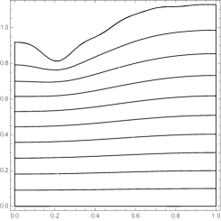
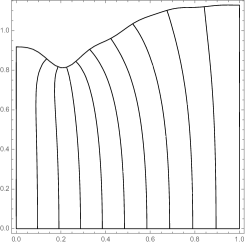
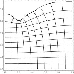
where and are computed using -FEM, and we tune the finite element approximation to ensure that (5.9) is approximately of the same order across all realizations of . One realization of with respective solutions and is shown in Figure 2.
The numerical experiments were carried out as follows:
-
(i)
We set , , and let in (5.1). We solve the problems (5.6) and (5.7) over QMC point sets with increasing number of cubature nodes and consider the error criteria
(5.10) where denotes the -dimensional QMC operator over cubature points. As the reference solution, we use the approximate QMC solution computed using . (The reference result is computed using a tailored lattice. In two cases the general lattice reference is available and the effect on the convergence curves is negligible.) The results are displayed in Figure 3a.
- (ii)
The QMC point sets for the above experiments were computed using the fast CBC algorithm using the same specifications as in Subsection 5.1. In order to utilize the a posteriori estimate introduced above, we remark that the boundary conditions of the numerical experiments are not the homogeneous Dirichlet zero boundary conditions analyzed in the earlier theory.
The observed rates are for : , : , : (see Figure 3a). The rate does not appear to depend on the dimension . The cone of convergence for shown in Figure 3c, is bounded by the rates (above) and (below). The general convergence patterns are clearly observed. The irregularities in the convergence behavior may be explained by the nonlinear QoI (compare with the experiment in Section 5.1) as well as the more complicated boundary conditions: the gradient term in the expression for the capacity appears to be sensitive to obtuse angles at the Dirichlet–Neumann interface for certain realizations of the random domain.
6 Conclusions
We analyzed the Poisson problem subject to domain uncertainty, employing a domain mapping approach in which the shape uncertainty is transferred onto a fixed reference domain. As a result, the coefficient of the transported PDE problem on the reference domain becomes highly nonlinear with respect to the stochastic variables. To this end, we developed a novel parametric regularity analysis for the transported problem subject to such diffusion coefficients. The parametric regularity analysis is an important ingredient in the design of tailored QMC rules and we demonstrated that these methods exhibit higher order cubature convergence rates when the random perturbation field is parameterized using the model introduced in [23] in which an infinite sequence of independent random variables enter the random field as periodic functions. The numerical results display that faster convergence in the stochastic fluctuations leads to faster QMC convergence in the computation of the PDE response, which is consistent with the theory.
Another novel feature of our work is the dimension truncation error analysis for the problem. Many studies in uncertainty quantification for PDEs with random coefficients exploit the parametric structure of the problem, using a Neumann series expansion to obtain dimension truncation error bounds. However, there have been several recent studies suggesting a Taylor series approach which is based on the parametric regularity of the problem [9, 11, 12]. The Taylor series approach can be used to obtain dimension truncation rates for non-affine parametric PDE problems, but a limitation of the aforementioned papers is that the parametric regularity bound needs to be of product-and-order dependent (POD) form in order for the Taylor-based approach to yield useful results. This issue is circumvented in the present paper by the use of a change of variables technique in order to transform our problem into a form in which the Taylor series approach can be used to produce improved dimension truncation error rates.
The results developed in this paper constitute important groundwork for other applications involving domain uncertainty such as domain shape recovery problems.
Acknowledgements
F. Y. Kuo and I. H. Sloan acknowledge the support from the Australian Research Council (DP210100831). This research includes computations using the computational cluster Katana supported by Research Technology Services at UNSW Sydney [24].
Appendix A Technical results
Lemma A.1.
Let , , , and . Let and be sequences of non-negative real numbers and suppose that
for all . Then
where we define, with ,
| (A.1) |
The result is sharp in the sense that all inequalities can be replaced by equalities. The result also extends to , i.e., we can remove the upper bounds on and .
Proof.
We prove the claim by induction with respect to the order of the multi-indices . The claim is resolved immediately for , so let us fix and suppose that the assertion holds for all multi-indices with order less than . Then
where we swapped the order of the sums over and . The inner sum over can be rewritten as
which can be further simplified using the identity (cf., e.g., [28, formula 26.8.23])
Hence
where we swapped the order of the sums over and and then carried out the change of variable . Changing the order of the sums again leads to
Relabeling to and applying the definition of yields the desired result.
We remark that if the inequalities for and the recursion on are replaced by equalities then all steps of the proof are equalities and so is the final formula. We also remark that the proof does not make any use of the upper bounds and , so the result extends trivially to the case . ∎
Let . It is interesting to note that if , for example, with , then the numbers (A.1) have the following representation in closed form:
These are so-called Delannoy numbers. We prove an upper bound for in general.
Lemma A.2.
Proof.
Let us first observe that the sequence can be represented using the recurrence and , ; see, e.g., entry A080599 in the On-line Encyclopedia of Integer Sequences (OEIS) and references therein. We also have and , .
We prove the claim (A.2) by induction with respect to the order of the multi-indices while utilizing the recursive characterization of sequence . We immediately see that (A.2) holds with equality when . Fix such that and suppose that the claim holds for all multi-indices with order less than . Then
as desired. ∎
Lemma A.3.
Let and let and be arbitrary sequences of real numbers. Then
| (A.3) |
Proof.
Moving the sum over further inside, we can write
| LHS of (A.3) | ||
as required. In the second equality we used the identity (cf., e.g., [28, formula 26.8.23])
In the third equality we introduced a change of variables . In the fourth equality we swapped the order of the sums. Finally we relabel to . ∎
Lemma A.4.
Let , and be sequences of non-negative real numbers satisfying
Then
The result is sharp in the sense that all inequalities can be replaced by equalities.
Proof.
We prove the claim by induction with respect to the multi-indices . The case is resolved immediately by observing that
as desired.
Fix and , and suppose that the claim holds for all pairs of multi-indices, with first multi-index of order and second multi-index . If , then the claim is trivially true, so we may assume in the following that . By letting be arbitrary, we find that
We introduce , , and . Then
Making use of the fact that (see [28, formula 26.8.25])
we obtain
where we used the change of variable in conjunction with the property for all . Recognizing the above expression as
concludes the proof. We remark that if the inequality for the recursion on is replaced by equality then all steps of the proof are equalities and so is the final formula. ∎
Lemma A.5.
Let be a constant and suppose that is a sequence of non-negative real numbers. Suppose that and
Then
where
| (A.4) |
The result is sharp in the sense that all inequalities can be replaced by equalities.
Proof.
The proof is carried out by induction with respect to the multi-indices . The base step is trivially true, so let us assume that is such that the claim holds for all multi-indices with order . Then the recurrence together with the induction hypothesis yields that
| (A.5) |
with
To simplify our presentation we abbreviate temporarily and . Then we can write
| (A.6) |
where we used Lemma A.3 in the third equality.
Reinserting the definitions of and , the inner sum over in (A) becomes
| (A.7) |
Substituting (A) and (A) into (A.5), we obtain
The result now follows from the definition of the sequence . ∎
We need to derive an upper bound for the sequences . In anticipation of this, let us define the auxiliary sequence
| (A.8) |
This sequence is listed as A003480 in The On-Line Encyclopedia of Integer Sequences (OEIS). We observe that this sequence satisfies the following property.
Lemma A.6.
The sequence defined by (A.8) satisfies
Proof.
Let . Then
as required. ∎
Remark. Lemma A.6 may be viewed as an extension of the renewal property of sequence A003480; see corresponding entry in the OEIS for further details.
We are now ready to state an upper bound for the sequence .
Proof.
The proof is carried out by induction with respect to the multi-indices . The base step , , is resolved by observing that and
Let with and suppose that the assertion holds for all multi-indices with . Then by separating out the term in (A.4) and applying the induction hypothesis to for , we obtain
where we used Lemma A.6 in the first equality. This completes the proof. ∎
It remains to obtain an estimate on the sequence.
Lemma A.8.
The sequence defined by (A.8) satisfies
Proof.
The claim is clearly true with equality when . If , then the sequence admits the following characterization (see the OEIS entry for this sequence and references therein):
from which the claim readily follows. ∎
References
- [1] L. V. Ahlfors. Conformal Invariants: Topics in Geometric Function Theory. Higher Mathematics Series. McGraw-Hill, 1973.
- [2] I. Babuška and P. Chatzipantelidis. On solving elliptic stochastic partial differential equations. Comput. Methods Appl. Mech. Engrg., 191:4093–4122, 2002.
- [3] J. E. Castrillón-Candás, F. Nobile, and R. F. Tempone. Analytic regularity and collocation approximation for elliptic PDEs with random domain deformations. Comput. Math. Appl., 71(6):1173–1197, 2016.
- [4] A. Cohen, Ch. Schwab, and J. Zech. Shape holomorphy of the stationary Navier–Stokes equations. SIAM J. Math. Anal., 50(2):1720–1752, 2018.
- [5] J. Dick, F. Y. Kuo, Q. T. Le Gia, D. Nuyens, and Ch. Schwab. Higher order QMC Petrov–Galerkin discretization for affine parametric operator equations with random field inputs. SIAM J. Numer. Anal., 52(6):2676–2702, 2014.
- [6] J. Dick, I. H. Sloan, X. Wang, and H. Woźniakowski. Good lattice rules in weighted Korobov spaces with general weights. Numer. Math., 103(1):63–97, 2006.
- [7] R. N. Gantner. Dimension truncation in QMC for affine-parametric operator equations. In A. B. Owen and P. W. Glynn, editors, Monte Carlo and Quasi-Monte Carlo Methods 2016, pages 249–264, Stanford, CA, 2018. Springer.
- [8] D. Gilbarg and N. S. Trudinger. Elliptic Partial Differential Equations of Second Order. Springer-Verlag, 2nd edition, 2001.
- [9] A. D. Gilbert, I. G. Graham, F. Y. Kuo, R. Scheichl, and I. H. Sloan. Analysis of quasi-Monte Carlo methods for elliptic eigenvalue problems with stochastic coefficients. Numer. Math., 142(4):863–915, 2019.
- [10] P. Grisvard. Elliptic Problems in Nonsmooth Domains. Pitman Publishing Inc., 1985.
- [11] P. A. Guth and V. Kaarnioja. Generalized dimension truncation error analysis for high-dimensional numerical integration: lognormal setting and beyond, 2022. Preprint at https://arxiv.org/abs/2209.06176.
- [12] P. A. Guth, V. Kaarnioja, F. Y. Kuo, C. Schillings, and I. H. Sloan. Parabolic PDE-constrained optimal control under uncertainty with entropic risk measure using quasi-Monte Carlo integration, 2022. Preprint at https://arxiv.org/abs/2208.02767.
- [13] H. Harbrecht. On output functionals of boundary value problems on stochastic domains. Math. Methods Appl. Sci., 33(1):91–102, 2010.
- [14] H. Harbrecht, V. Karnaev, and M. Schmidlin. Quantifying domain uncertainty in linear elasticity. Technical Report 2023-06, Fachbereich Mathematik, Universität Basel, Switzerland, 2023.
- [15] H. Harbrecht, M. Peters, and M. Siebenmorgen. Analysis of the domain mapping method for elliptic diffusion problems on random domains. Numer. Math., 134(4):823–856, 2016.
- [16] H. Harbrecht and M. Schmidlin. Multilevel quadrature for elliptic problems on random domains by the coupling of FEM and BEM. Stoch. Partial Differ. Equ. Anal. Comput., 2021. to appear.
- [17] H. Harbrecht, R. Schneider, and Ch. Schwab. Sparse second moment analysis for elliptic problems in stochastic domains. Numer. Math., 109(3):385–414, 2008.
- [18] G. H. Hardy, J. E. Littlewood, and G. Pólya. Inequalities. Cambridge University Press, Cambridge, UK, 1934.
- [19] R. Hiptmair, L. Scarabosio, C. Schillings, and Ch. Schwab. Large deformation shape uncertainty quantification in acoustic scattering. Adv. Comput. Math., 44(5):1475–1518, 2018.
- [20] L. Hörmander. An Introduction to Complex Analysis in Several Variables. North-Holland, 3rd edition, 1990.
- [21] C. Jerez-Hanckes, Ch. Schwab, and J. Zech. Electromagnetic wave scattering by random surfaces: Shape holomorphy. Math. Models Methods Appl. Sci., 27(12):2229–2259, 2017.
- [22] V. Kaarnioja, F. Y. Kuo, and I. H. Sloan. Lattice-based kernel approximation and serendipitous weights for parametric PDEs in very high dimensions. To appear in: A. Hinrichs, P. Kritzer, F. Pillichshammer (eds.). Monte Carlo and Quasi-Monte Carlo Methods 2022. Springer Verlag.
- [23] V. Kaarnioja, F. Y. Kuo, and I. H. Sloan. Uncertainty quantification using periodic random variables. SIAM J. Numer. Anal., 58(2):1068–1091, 2020.
- [24] Katana. Published online, 2010. DOI:10.26190/669X-A286.
- [25] D. Kressner and C. Tobler. Low-rank tensor Krylov subspace methods for parametrized linear systems. SIAM J. Matrix Anal. Appl., 32(4):1288–1316, 2011.
- [26] F. Y. Kuo, Ch. Schwab, and I. H. Sloan. Quasi-Monte Carlo finite element methods for a class of elliptic partial differential equations with random coefficients. SIAM J. Numer. Anal., 50(6):3351–3374, 2012.
- [27] P. S. Mohan, P. B. Nair, and A. J. Keane. Stochastic projection schemes for deterministic linear elliptic partial differential equations on random domains. Internat. J. Numer. Methods Engrg., 85(7):874–895, 2011.
- [28] F. W. J. Olver, A. B. Olde Daalhuis, D. W. Lozier, B. I. Schneider, R. F. Boisvert, C. W. Clark, B. R. Miller, B. V. Saunders, H. S. Cohl, M. A. McClain, and eds. NIST Digital Library of Mathematical Functions. Release 1.1.6 of 2022-06-30., http://dlmf.nist.gov/.
- [29] T. H. Savits. Some statistical applications of Faa di Bruno. J. Multivariate Anal., 97(10):2131–2140, 2006.
- [30] I. H. Sloan and P. J. Kachoyan. Lattice methods for multiple integration: Theory, error analysis and examples. SIAM J. Numer. Anal., 24(1):116–128, 1987.
- [31] D. Xiu and D. M. Tartakovsky. Numerical methods for differential equations in random domains. SIAM J. Sci. Comput, 28(3):1167–1185, 2006.