The Kochawave curve, a variant of the Koch curve

Abstract

This paper presents the construction and some properties of the Kochawave curve, a simple and asymmetrical variant of the Koch curve.

1 Introduction

The Koch curve [9] is a well-known fractal described in 1904 by the Swedish mathematician Helge von Koch [2].

Since then, many variants of the Koch curve have been described in the literature, such as the Cesàro fractal [8] and the quadratic Koch curve [1], just to name two (see Li [3], Rani [4], Ventrella [6] and Wikipedia [9] for other variants).

We present here another variant of the Koch curve: the Kochawave curve, mentioned and named by Wahl [7]. The Kochawave curve has a simple and asymmetrical structure, and as its name suggests, looks like a wave.

2 Construction

The Kochawave curve is a fractal curve. We describe four ways to construct it.

2.1 Construction with segments

The Kochawave curve can be constructed starting from one unit segment, and iteratively replacing each line segment $\overrightarrow{AE}$ with four line segments $\overrightarrow{AB}$, $\overrightarrow{BC}$, $\overrightarrow{CD}$, $\overrightarrow{DE}$ such that the points $A$, $B$, $D$ and $E$ are colinear and equally spaced (and appear in that order) and $DEC$ forms an equilateral triangle (see figure 1).

Figure 1: The construction rule for the Kochawave curve

The Koch curve has a similar construction rule, except that there $BDC$ forms an equilateral triangle (see figure 2).

Figure 2: The construction rule for the Koch curve

The first four iterations of the construction of the Kochawave curve are depicted in figure 3.

Figure 3: The first four iterations of the Kochawave curve

The Kochawave curve is the limiting figure as the iterations continue indefinitely (see figure 4).

Figure 4: The Kochawave curve

2.2 Construction with triangles

We can construct three entangled Kochawave curves starting from one unit sided equilateral triangle, and iteratively replacing each equilateral triangle, say of side length $w$, with four equilateral triangles, of side lengths $w/3$, $w/3$, $w/3$ and $w/\sqrt{3}$, respectively, with the same orientation as in the original triangle, as depicted in figure 5.

Figure 5: The construction rule for the three entangled Kochawave curves

The first four iterations of the construction of the three entangled Kochawave curves are depicted in figure 6.

Figure 6: The first four iterations of the three entangled Kochawave curves

The three entangled Kochawave curves are the limiting figure as the iterations continue indefinitely (see figure 7). We see that the limiting figure is made up of three copies of the Kochawave curve we saw in figure 4.

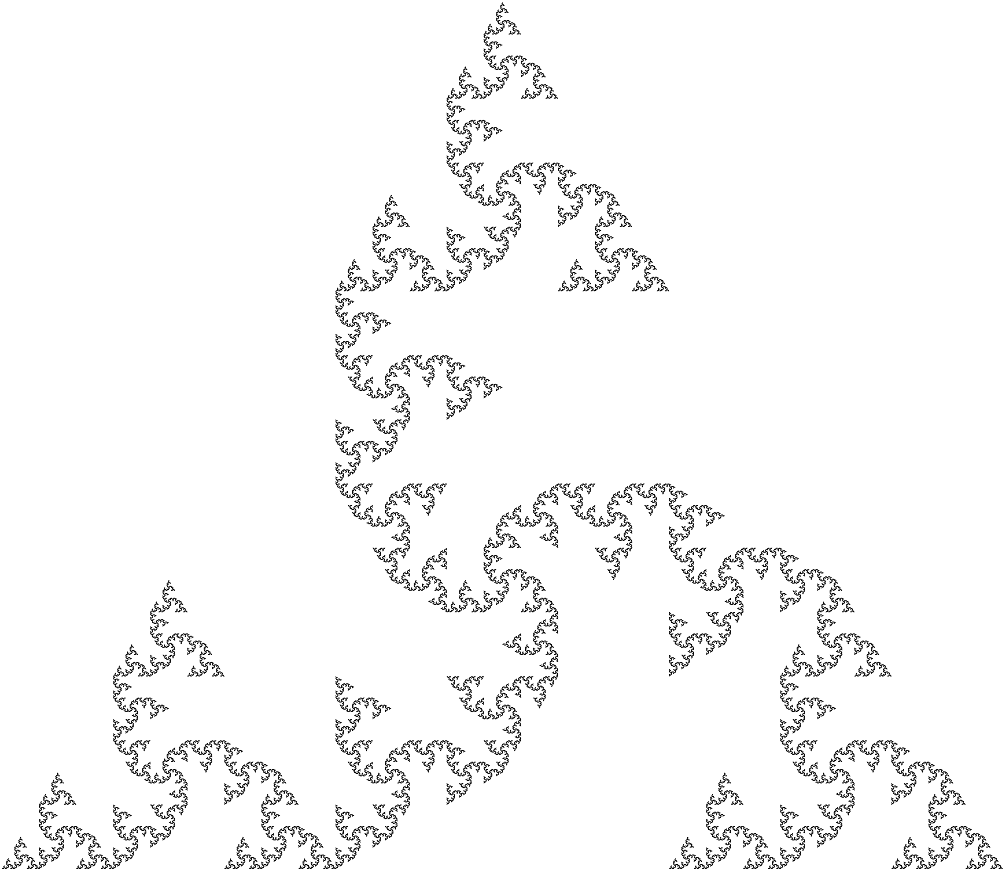
Figure 7: The three entangled Kochawave curves

2.3 Construction with an L-system

We can express the Kochawave curve with the following L-system:

• alphabet: $\{S,\ *\ ,\ /,\ +\}$,

• axiom: $S$,

• unique production rule: $S\rightarrow S\ *\ S\ /\ S\ +\ S$.

The alphabet is to be interpreted as described in the following table.

Symbol	Interpretation
$S$	Draw one step forward.
$*$	Turn $30^{\circ}$ left and stretch the next steps by $\sqrt{3}$.
$/$	Turn $150^{\circ}$ right and stretch the next steps by $1/\sqrt{3}$.
$+$	Turn $120^{\circ}$ left.

The length of the $k^{th}$ step is $\sqrt{3}^{u_{k-1}}$, where $u_{k-1}$ denotes the number of $1$’s in the base-4 representation of $k-1$.

2.4 Numerical construction

Let:

$$z_{0}=0,\ z_{k+1}=z_{k}+\frac{(1+\omega)^{u_{k}}}{\omega^{2v_{k}}}$$

where $\omega=e^{\frac{i\pi}{3}}$, and $u_{k}$ and $v_{k}$ denote the number of $1$’s and of $2$’s, respectively, in the base-4 expansion of $k$.

The coordinates of the sequence of points $\{z_{n}\}_{n\geq 0}$ on a hexagonal lattice are given by the OEIS [5] sequences A335380 and A335381.

The set of endpoints of the segments after $n$ iterations of the construction described in section 2.1 is given by:

$$K_{n}=\left\{\frac{z_{k}}{3^{n}},\ k=0\mathinner{\ldotp\ldotp}4^{n}\right\}$$

The first few sets are depicted in figure 8.

Figure 8: The sets of points $K_{0}$ to $K_{3}$ (in blue)

As $z_{4n}=3z_{n}$, $K_{n}\subset K_{n+1}$.

The closure of the limit $\lim_{n\to\infty}K_{n}$ is the Kochawave curve.

3 Properties

3.1 Length of the Kochawave curve

After $n$ iterations of the construction described in section 2.1, the length $L_{n}$ of the structure is given by:

$$L_{n}=\left(1+\frac{1}{\sqrt{3}}\right)^{n}$$

Note that $L_{0}=1$ as we started with a unit segment.

As $\lim_{n\to\infty}L_{n}=\infty$, the Kochawave curve has infinite length.

3.2 Area of the three entangled Kochawave curves

After $n$ iterations of the construction described in section 2.2, the area $T_{n}$ of the structure is given by:

$$T_{n}=\frac{\sqrt{3}}{4}\cdot\left(\frac{2}{3}\right)^{n}$$

Note that $T_{0}=\frac{\sqrt{3}}{4}$ as we started with a unit sided equilateral triangle.

As $\lim_{n\to\infty}T_{n}=0$, the three entangled Kochawave curves have empty area. By contrast, the Koch antisnowflake has positive area.

3.3 Area of the Kochawave curve

After $n$ iterations of the construction described in section 2.1, the area $A_{n}$ enclosed between the structure and the initial segment satisfies:

$$3A_{n}+T_{n}=\frac{\sqrt{3}}{4}$$

Hence:

$$A_{n}=\frac{\frac{\sqrt{3}}{4}-T_{n}}{3}=\frac{1}{4\sqrt{3}}\cdot\left[1-\left(\frac{2}{3}\right)^{n}\right]$$

The area $A$ of the Kochawave curve is given by:

$$A=lim_{n\to\infty}A_{n}=\frac{1}{4\sqrt{3}}$$

This is one third of the area of a unit sided equilateral triangle, and indeed, we can divide an equilateral triangle into three Kochawave curves (see figure 9).

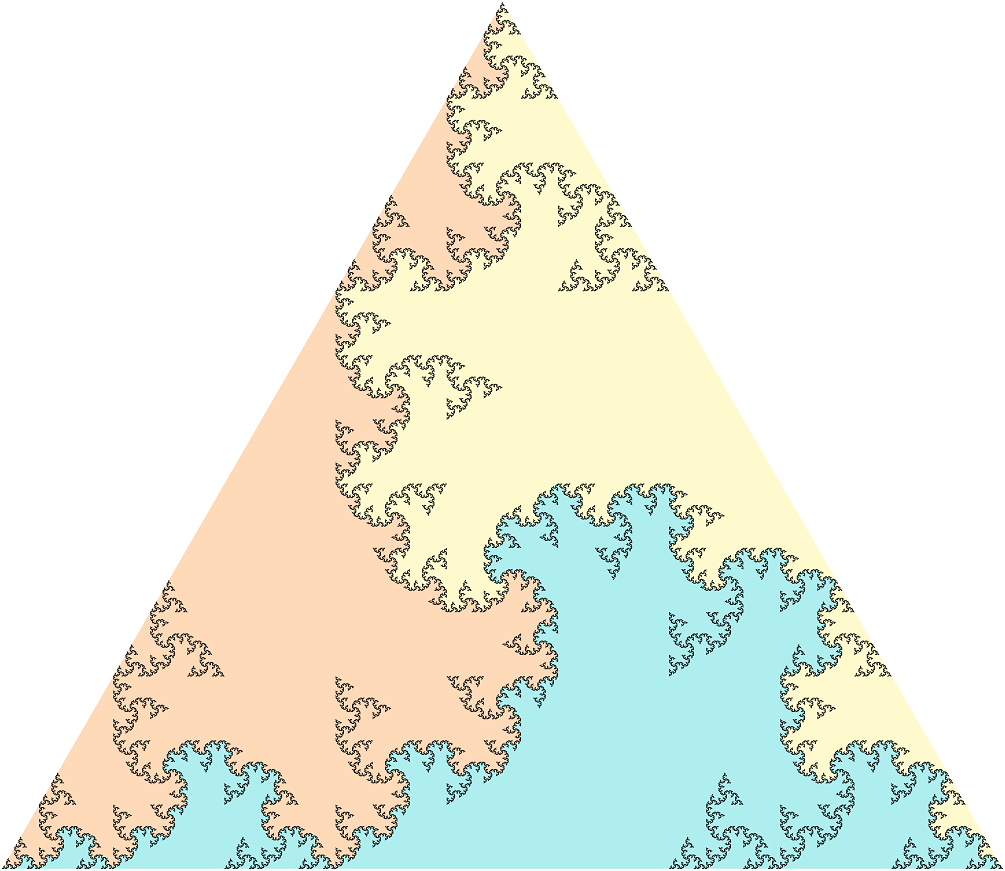
Figure 9: An equilateral triangle divided into three Kochawave curves

3.4 Height of the Kochawave curve

After $n$ iterations of the construction described in section 2.1, the height $H_{n}$ of the structure is given by:

$$H_{n}=\max_{p\in K_{n}}Im(p)=\left\{\begin{array}[]{cl}0&\mathrm{if}\ n=0\\ \frac{1}{2\sqrt{3}}&\mathrm{if}\ n=1\\ \frac{2}{3\sqrt{3}}&\mathrm{if}\ n>1\end{array}\right.$$

The height $H$ of the Kochawave curve is given by:

$$H=lim_{n\to\infty}H_{n}=\frac{2}{3\sqrt{3}}$$

The leftmost point of height $H$ has position $\frac{4+4\omega}{9}$.

The rightmost point of height $H$ has position $\frac{5+4\omega}{9}$.

3.5 Centroid of the Kochawave curve

We can dissect a Kochawave curve, say of weight $1$, into five parts:

• one copy of the curve of weight $\frac{1}{3}$,

• three copies of the curve of weight $\frac{1}{9}$,

• one triangle of weight $\frac{1}{3}$.

as depicted in figure 10 (this dissection derives directly from the construction described in section 2.1).

This leads to the following linear equation for the centroid $m$ of the Kochawave curve:

$$m=\frac{1}{9}\cdot\frac{m}{3}+\frac{1}{3}\cdot\frac{1+(1+\omega)m}{3}+\frac{1}{9}\cdot\frac{2+\omega-\omega m}{3}+\frac{1}{9}\cdot\frac{2+m}{3}+\frac{1}{3}\cdot\frac{\frac{5}{3}+\frac{\omega}{3}}{3}$$

Hence the centroid $m$ of the Kochawave curve is:

$$m=\frac{59+17\omega}{111}$$

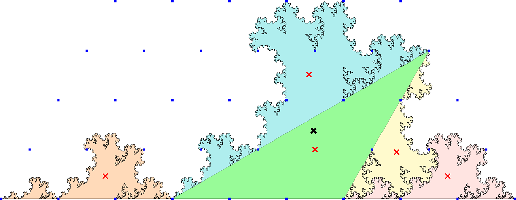
Figure 10: The dissection of a Kochawave curve into five parts (red marks correspond to centroids of parts, the black mark corresponds to the centroid $m$)

3.6 Volume of solid of revolution

The volume $V$ of the solid of revolution of the Kochawave curve around its base unit segment satisfies:

$$V=2\pi\cdot Im(m)\cdot A=\frac{17}{444}\pi$$

3.7 Hausdorff dimension of the Kochawave curve

The Kochawave curve satisfies the open set condition; its Hausdorff dimension $d$ is the unique real solution of the following equation:

$$\frac{1}{3^{d-1}}+\frac{1}{\sqrt{3}^{d}}=1$$

and has exact value:

$$d=2\cdot\frac{\log\frac{1+\sqrt{13}}{2}}{\log 3}$$

which is approximately $1.518$.

3.8 Symmetries

Contrary to the Koch curve, the Kochawave curve has no particular symmetry (see figure 4). As for the Koch antisnowflake, the three entangled Kochawave curves have 3-fold rotational symmetry (see figure 7).

3.9 Cantor set underlying the Kochawave curve

When building the Kochawave curve starting from one unit segment as described in section 2.1, the remainder of this initial segment forms a ternary Cantor set. This property is shared with the Koch curve.

Figure 11: Remainder of the initial segment after one to four iterations (in blue)

3.10 Connectivity

The Kochawave curve and the three entangled Kochawave curves are simply connected.

3.11 Left boundary

During the construction of the Kochawave curve seen in section 2.1, we notice closed loops made of equilateral triangles. Each of these equilateral triangles will give rise to three small entangled Kochawave curves, and participate in the fractal nature of the Kochawave curve (see figure 12).

Figure 12: The closed loops after four iterations of the construction of the Kochawave curve (in green)

If we remove these closed loops, we obtain a simple curve $\mathcal{C}$, with the same area (see section 3.3) as the corresponding Kochawave curve. The curve $\mathcal{C}$ can be split into two parts, $AO$ and $BO$ (where $O$ is the center of the equilateral triangle with base $AB$); $AO$, when rotated $120^{\circ}$ counterclockwise around $O$, gives $BO$ (see figure 13).

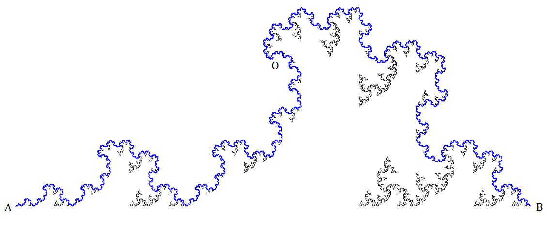
Figure 13: The curve $\mathcal{C}$ (in blue)

We can construct the curve $\mathcal{C}$ starting with a single black unit segment, and applying the substitution rules depicted in figure 14.

Figure 14: The construction rules for the curve $\mathcal{C}$

After $n$ iterations, the total length of the construction, say $c_{n}$, satisfies:

$$\left(\frac{1}{2}+\frac{1}{\sqrt{3}}\right)^{n}\leq c_{n}\leq\left(1+\frac{1}{\sqrt{3}}\right)^{n}$$

These inequalities are deduced from the two construction rules in figure 14.

As $\frac{1}{2}+\frac{1}{\sqrt{3}}>1$, $\lim_{n\to\infty}c_{n}=\infty$, and the curve $\mathcal{C}$ has infinite length.

4 Tessellations of the plane

4.1 Tiles

We describe five tiles whose edges are made of two, three or four Kochawave curves. These tiles can cover the Euclidian plane (see section 4.2).

4.1.1 Biface antisymmetrical tile

The biface antisymmetrical tile is made of two Kochawave curves arranged head to tail as depicted in figure 15.

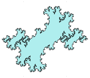
Figure 15: The biface antisymmetrical tile

This tile can be obtained by arranging $2^{k-1}$ copies of the rhomboid tile (see figure 18) scaled by a factor $1/3^{k}$ for $k\geq 1$.

4.1.2 Biface symmetrical tile

The biface symmetrical tile is made of two Kochawave curves arranged symmetrically as depicted in figure 16.

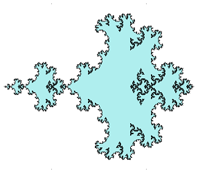
Figure 16: The biface symmetrical tile

This tile can be obtained by arranging $2^{k-1}$ copies of the dart tile (see figure 19) scaled by a factor $1/3^{k}$ for $k\geq 1$.

4.1.3 Triangular tile

The triangular tile is made of three Kochawave curves arranged around an equilateral triangle as depicted in figure 17.

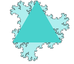
Figure 17: The triangular tile

4.1.4 Rhomboidal tile

The rhomboidal tile is made of four Kochawave curves arranged around a rhomboid as depicted in figure 18.

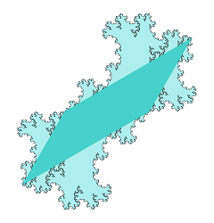
Figure 18: The rhomboidal tile

4.1.5 Dart tile

The dart tile is made of four Kochawave curves arranged around a dart as depicted in figure 19.

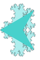
Figure 19: The dart tile

4.2 Tessellations

We describe five ways to cover the Euclidian plane with the tiles seen in section 4.1.

4.2.1 With biface antisymmetrical tiles

We can cover the plane with copies of the biface antisymmetrical tile in one size (see figure 20). This covering is periodic.

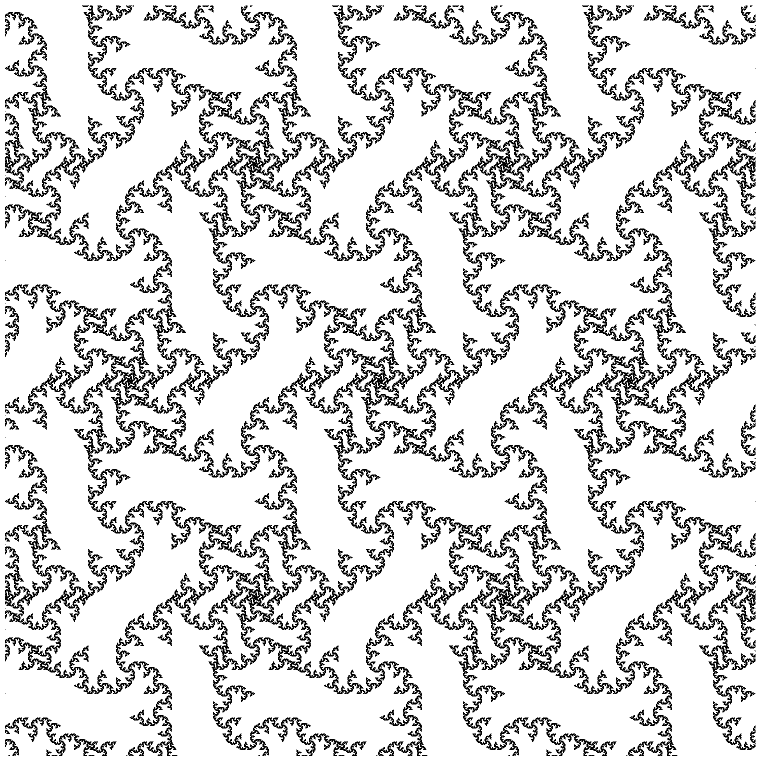
Figure 20: Covering the plane with biface antisymmetrical tiles

4.2.2 With biface antisymmetrical tiles

We can cover the plane with copies of the biface antisymmetrical tile in one size (see figure 21). This covering is periodic.

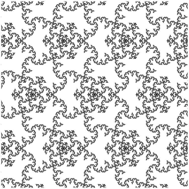
Figure 21: Covering the plane with biface symmetrical tiles

4.2.3 With triangular tiles

We can cover the plane with copies of the triangular tile in one size (see figure 22). This covering is periodic.

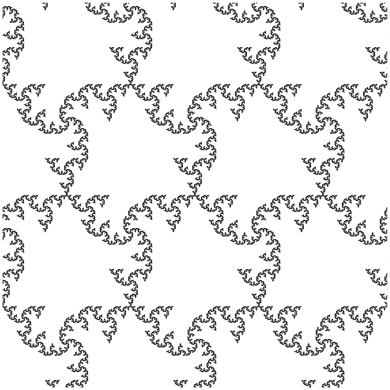
Figure 22: Covering the plane with triangular tiles

4.2.4 With rhomboidal tiles

We can cover the plane with copies of the rhomboidal tile scaled by factors $3^{k}$ for $k\in\mathbb{Z}$ (see figure 23). This covering has scale invariance.

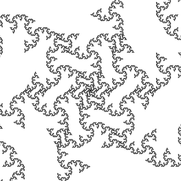
Figure 23: Covering the plane with rhomboidal tiles

4.2.5 With dart tiles

We can cover the plane with copies of the dart tile scaled by factors $3^{k}$ for $k\in\mathbb{Z}$ (see figure 24). This covering has scale invariance.

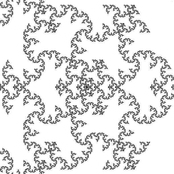
Figure 24: Covering the plane with dart tiles

5 Acknowledgments

I would like to express my very great appreciation to Jörg Arndt, Kevin Ryde and Neil Sloane for their valuable and constructive suggestions.

References

- [1] Robert Ferréol, “Quadratic Koch curve”, https://mathcurve.com/fractals/kochquadratique/kochquadratique.shtml
- [2] Helge von Koch, “Sur une courbe continue sans tangente, obtenue par une construction géométrique élémentaire”, https://zbmath.org/?q=an%3A35.0387.02; 1904
- [3] Yao-Qiang Li, “Generalized Koch curves and Thue-Morse sequences”, https://arxiv.org/abs/2009.14488
- [4] Mamta Rani, Riaz Ul Haq, Deepak Kumar Verma, “Variants of Koch curve: A Review”, https://www.researchgate.net/publication/322799091
- [5] The OEIS Foundation Inc. (2022), “The On-Line Encyclopedia of Integer Sequences”, published electronically at https://oeis.org
- [6] Jeffrey Ventrella, “Brain-filling Curves - A Fractal Bestiary”, http://www.brainfillingcurves.com/; 2012
- [7] Bernt Rainer Wahl, “The Fractal Explorer”, http://www.wahl.org/fe/HTML_version/link/FE3W/c3.htm#koch; 2006
- [8] Eric W. Weisstein, “Cesàro Fractal. From MathWorld—A Wolfram Web Resource”, https://mathworld.wolfram.com/CesaroFractal.html
- [9] Wikipedia, The Free Encyclopedia, “Koch snowflake”, https://en.wikipedia.org/wiki/Koch_snowflake