Neural Network-based CUSUM for Online
Change-point Detection

Abstract

Change-point detection, detecting an abrupt change in the data distribution from sequential data, is a fundamental problem in statistics and machine learning. CUSUM is a popular statistical method for online change-point detection due to its efficiency from recursive computation and constant memory requirement, and it enjoys statistical optimality. CUSUM requires knowing the precise pre- and post-change distribution. However, post-change distribution is usually unknown a priori since it represents anomaly and novelty. When there is a model mismatch with actual data, classic CUSUM can perform poorly. While likelihood ratio-based methods encounter challenges in high dimensions, neural networks have become an emerging tool for change-point detection with computational efficiency and scalability. In this paper, we introduce a neural network CUSUM (NN-CUSUM) for online change-point detection. We also present a general theoretical condition when the trained neural networks can perform change-point detection and what losses can achieve our goal. We further extend our analysis by combining it with the Neural Tangent Kernel theory to establish learning guarantees for the standard performance metrics, including the average run length (ARL) and expected detection delay (EDD). The strong performance of NN-CUSUM is demonstrated in detecting change-point in high-dimensional data using both synthetic and real-world data.

1 Introduction

Quick detection of unknown change in the distribution of sequential data, known as change-point detection, is a crucial issue in statistics and machine learning [1, 2, 3, 4]. It is often triggered by an event that may lead to significant consequences, making timely detection critical in minimizing potential losses. For instance, a change-point could arise when production lines become unmanageable. Early detection and remediation by practitioners would result in lesser loss. With the rapidly growing amount of streaming data, the change-point detection is applicable to practical problems across diverse fields such as epidemiology [5], social network analysis [6], and scientific imaging [7].

In the modern high-volume and complex data era, across numerous applications, sequential data is collected over networks with higher dimensionality and more complex distributions than before. Therefore, the conventional setting of the change-point detection problem has been surpassed in scope by its modern version. The assumptions in the classical methodologies are possibly too restrictive to tackle the newly occurring challenges, including the high-dimensionality and complex spatial and temporal dependence of sequential data.

Various methods have been proposed to address the challenges above. Deep learning architectures (e.g., RNN, CNN, autoencoder) were often used to learn complex spatio-temporal dependence in the data for change-point detection [8, 9, 10]. Moustakides and Basioti [11] aimed to develop a suitable optimization framework for training neural network-based estimates of the likelihood ratio or its transformations where the estimates can be used for change-point detection and hypothesis testing. Detecting changes by statistics generated by online training of neural networks has been recently studied in a few previous works. Lee et al. [12] consider a similar approach of using a trained neural network statistic-based CUSUM procedure for change-point detection. Hushchyn et al.  [13] introduces online neural network classification (ONNC) and online neural network regression (ONNR), which is based on sequentially applying neural networks for classification or regression for comparing the current batch of data with the immediate past batch of data, to obtain the detection statistic with separating training and testing. However, prior works did not present theoretical guarantees of the algorithms; here, we generalize the prior works by considering general losses, presenting a formal theoretical guarantee with extensive numerical experiments. Moreover, ONNC and ONNR [13] can be viewed as Shewhart chart type (without accumulating history information and with short memory) rather than a CUSUM-type of algorithm (accumulating all past history information through the recursion); it is known that Shewhart may be good at detecting larger changes but not small changes, while CUSUM procedures are known to be sensitive to small changes and enjoy asymptotic optimality properties.

In this paper, we leverage neural networks to efficiently detect the change-point in the streaming data with high-dimensionality and complex spatial-temporal correlations. The starting point is to convert online change-point detection into a classification problem, of which neural networks are highly capable. Now that the explicit form of the distribution and the log-likelihood ratio is unknown, neural networks benefit us in that the training loss of the neural networks will approximate the underlying true log-likelihood ratio between pre- and post-change distributions. Further, we couple the loss from the neural networks with CUSUM recursion. We present the statistical performance guarantee for two statistical metrics, the average run length (ARL) and the expected detection delay (EDD) for the proposed algorithm, combining renewal theory for stopping time analysis and neural-tangent-kernel (NTK) analysis. We summarize the idea as an efficient online training procedure and design extensive simulations and empirical experiments to thoroughly discuss the proposed method and both conventional and state-of-art methods.

2 Preliminaries

Consider a sequence of observations $\{x_{t}\in\mathbb{R}^{d}:t=1,2,\ldots\}$. At some point, there may be a change-point $k$ such that the distribution of the data shifted from $f_{0}$ to $f_{1}$, which can be formulated as the following composite sequential hypothesis test

$$\begin{split}H_{0}:&\quad x_{1},x_{2},\ldots,x_{t},\ldots\overset{\mathrm{iid}}{\sim}f_{0},\\ H_{1}:&\quad x_{1},x_{2},\ldots,x_{k}\overset{\mathrm{iid}}{\sim}f_{0},\quad x_{k+1},\ldots x_{t},\ldots\overset{\mathrm{iid}}{\sim}f_{1},\end{split}$$ (1)

where $f_{0}$ and $f_{1}$ represent the pre- and post-change distributions, respectively. The expectations under $f_{0}$ or $f_{1}$ are denoted by $\mathbb{E}_{0}[\cdot]$ and $\mathbb{E}_{1}[\cdot]$, respectively. We assume that pre-change data under $f_{0}$ are adequate to converge any interested pre-change statistics. We call the pool of pre-change data in the training process as pilot sequence. This assumption commonly holds since, in practice, the process is mostly pre-change, which allows the sufficient collection of reference data to represent the “normal” state. Another assumption is that the pre-change distribution $f_{0}$ is known, which can be viewed to be equivalent to sufficient pre-change data up to some estimation error.

The classic CUSUM procedure is popular possibly due to its computationally efficient recursive procedure, and enjoys various optimality properties (see, e.g., a survey [4]). CUSUM detects the change using the exact likelihood ratio through the recursion $S_{t}^{\rm C}=\left(S_{t-1}^{\rm C}+\log({f_{1}(x_{t})}/{f_{0}(x_{t})})\right)^{+}.$ where $S_{0}^{\rm C}=0$, and $(x)^{+}=\max\{x,0\}$. CUSUM procedure is a stopping time $\tau_{\rm C}=\inf\{t:S_{t}^{\rm C}>b\},$ where $b>0$ is the pre-specified threshold. However, the post-change distribution $f_{1}$ is usually unknown and in practice, when the assumed distributions deviate from the true distributions, CUSUM may suffer from performance degradation.

3 Neural Network CUSUM

In this section, we propose the Neural Network (NN)-CUSUM procedure. We consider a neural network function $g_{\theta}(x):\mathbb{R}^{d}\rightarrow\mathbb{R}$, parameterized by $\theta$. The network sequentially takes a pre-change distributed pilot sequence and an unknown distributed online sequence as input. During training, we convert the change-point detection problem into a binary classification problem and label data from the pilot and online sequences with $y_{i}=0$ and $y_{i}=1$, respectively. We feed the labeled data into the neural network and train it using a carefully crafted logistic loss function. Subsequently, the neural network computes the logistic loss for each data point in the pilot and online sequences for every time step. We employ the difference between the average logistic function values of the pilot and online sequences as the sequential statistics for detecting change-point. Figure 1 visualize the proposed framework.

The stopping time $\tau$ is crucial in the sequential hypothesis testing approach for detecting changes in a streaming dataset. It indicates the time to terminate the data stream and declares the occurrence of a distribution shift prior to time $\tau$. We borrow the conventional exact CUSUM framework in our proposed scheme to construct the stopping time. However, we replace the exact log-likelihood ratio with an approximation from a neural network. Before presenting our approach’s specifics, we provide an overview of the exact CUSUM procedure and other relevant methods.

3.1 Training

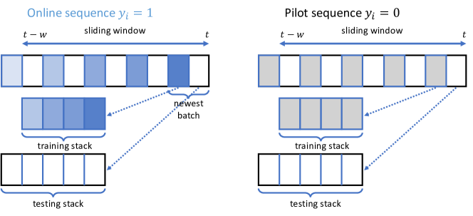
Figure 1: Illustration of the NN-CUSUM procedure, figure reproduced from [12]. When the newest batch from the streaming data (treated with label $y_{i}=1$) is received, it is divided to put into the training stack and the testing stack, respectively (the oldest samples are purged from the stacks). The neural network inherited from the previous $t$ will be updated using a stochastic gradient descent algorithm for one-pass through the freshened training stack data. The updated neural network is then used to compute the test statistic for data in the freshened testing stack data. The label $y_{i}=0$ (from pilot samples) is constructed in a completely parallel way. The training/testing stack sizes are hyper-parameters to be tuned in practice to achieve a good detection performance.

The training of the neural network is conducted via stochastic gradient descent (SGD) updates of the neural network parameter $\theta$ on the training stack. As is shown in Figure 1, the training stack contains multiple mini-batches of data in $[t-w,t]$ window from arriving data stream. Within the window, we use a fraction of $\alpha$ samples for training and a fraction of $1-\alpha$ samples for testing. This gives the online training data set $\widetilde{X}_{t}^{\rm tr}$ and the online test data set $\widetilde{X}_{t}^{\rm te}$, with a size of $\alpha w$ and $(1-\alpha)w$, $\alpha\in(0,1)$, respectively. The window length $w$ and training split fraction $\alpha$ are algorithm parameters.

The sliding window moves forward with stride $s$, $s\leq w$. Half of the stride is put into the training stack and the other half is put into the testing stack. Recall that the data in the online sequence $X_{t}$ are labeled 1 and the data in the pilot sequence $\widetilde{X}_{t}$ are labeled 0. We updated the pilot sequence by drawing randomly from pilot samples.

Let $\varphi(x,\theta)$ be the neural network function that maps from $\mathcal{X}\subset\mathbb{R}^{D}\to\mathbb{R}$ and $\theta$ is the network parameter. Consider training the neural network using the following general loss, which is computed from the combined training split of arrival and pilot samples on the window $D_{t}^{\rm tr}:=X_{t}^{\rm tr}\cup\widetilde{X}_{t}^{\rm tr}=\{x_{i}\}_{i=1}^{2m}$, $m=\alpha w$, labeled by $y_{i}=1$ if $x_{i}\in X_{t}^{\rm tr}$ and $y_{i}=0$ if $x_{i}\in\widetilde{X}_{t}^{\rm tr}$,

$$\ell(\theta;D_{t}^{\rm tr})=\frac{1}{m}\sum_{i=1}^{2m}l(\varphi(x_{i},\theta),y_{i}),$$ (2)

We may use different training loss functions. The per-sample loss function $l(u,y)$ can be chosen to be different losses. For the logistic loss,

$$l_{\rm logit}(u,y)=y\log(1+e^{-u})+(1-y)\log(1+e^{u}).$$ (3)

Apart from the logistic loss, we also consider the $\ell^{2}$-loss, defined as

$$l_{\ell^{2}}(u,y)=\frac{1}{2}\left(y(u-1)^{2}+(1-y)(u+1)^{2}\right),$$ (4)

and the linearized version of the logit loss, motivated by the MMD test statistic [14], as

$$l_{\rm MMD}(u,y)=-yu+(1-y)u.$$ (5)

Here we assume that the SGD training to minimize (2) is conducted on $D_{t}^{\rm tr}$ for each window indexed by $t$ separately from scratch, and the trained network parameter is denoted as $\hat{\theta}_{t}$.

The choice of the loss function is motivated by the fact that the functional global minimizer gives the log density ratio: For $f_{0}$ and $f_{1}$, which are probability densities on $\mathbb{R}^{d}$, let

$$\ell[\varphi]=\int\log(1+e^{\varphi(x)})f_{0}(x)dx+\int\log(1+e^{-\varphi(x)})f_{1}(x)dx,$$

which is the population loss, then $\ell[\varphi]$ is minimized at $\varphi^{*}=\log(f_{1}/f_{0})$. One can verify that the functional $\ell[\varphi]$ is convex with respect to perturbation in $\varphi$. By that $\frac{\delta\ell}{\delta\varphi}=\frac{f_{0}e^{\varphi}-f_{1}}{1+e^{\varphi}}$, we know $\delta\ell/\delta\varphi$ vanishes when $e^{\varphi}=f_{1}/f_{0}$, that is $\varphi=\varphi^{*}$, and this is a global minimum of $\ell[\varphi]$.

In our implementation, the neural network parameter $\theta$ is initialized at time zero and then updated by SGD (e.g., Adam [15]) through batches of training samples in a sliding training window. Newly arrived data stay in the stack for $w/s$ steps. We trained the network on the training stack in every $k$ step. Thus, on average, each data sample has been used $(w/s)/k$ times for training $\theta$. The number $(w/s)/k$ can be viewed as a hyperparameter indicating an effective number of epochs.

3.2 Testing and CUSUM

At time $t$ of the arrival stream of $X_{t}$, suppose the trained neural network provide a test function $g_{\hat{\theta}_{t}}(x)$, where $\hat{\theta}_{t}$ denotes the dependence on the trained neural network parameter which also depends on time index $t$. For logistic and $\ell_{2}$ loss, we set the function $g_{\hat{\theta}_{t}}=\varphi(\cdot,\hat{\theta}_{t})$. For MMD loss, $g_{\hat{\theta}_{t}}$ will be specified in Section 4.3. We compute the sample average on the testing windows $X^{\rm te}_{t}$ and $\widetilde{X}^{\rm te}_{t}$ (recall that $\tilde{X}_{t}\sim f_{0}$ are drawn sequentially from the pilot samples):

$$\eta_{t}:=\frac{1}{(1-\alpha)w}\left[\sum_{x\in X^{\rm te}_{t}}g_{\hat{\theta}_{t}}(x)-\sum_{x\in\widetilde{X}^{\rm te}_{t}}g_{\hat{\theta}_{t}}(x)\right].$$ (6)

where $\alpha\in(0,1)$ describes the proportion of the data in the window used for testing; so $\alpha w$ data are used for updating the training stack.

Starting with $S_{0}=0$, the recursive CUSUM is computed as

$$S_{t}=(S_{t-1}+\eta_{t}-d)^{+},$$ (7)

where $d>0$ is a small constant called the “drift” to ensure that the expected value of the drift term is negative before the change, and positive after the change; we will give the condition of the test function that can satisfy this in the following section.

For simplicity, our algorithm computes $\eta_{t}$ at intervals of $s$ (for “stride”), which is the size of mini-batches of loading the stream data, e.g. $s=10$; in the extreme case, $s=1$. When $s=w$, the sliding window contains completely non-overlapping data. The test statistic $S_{t}$ is computed with stride $s$. For some pre-specified threshold $b>0$, the detection procedure is by the stopping time

$$\tau=\inf\{t:S_{t}>b\}.$$ (8)

4 Performance guarantee

For simplicity, we analyze a simplified setting of online NN training where the sliding window $(t-w,t]$ is taken without overlapping, that is the stride $s=w$. For change-point detection, after training, the increment in CUSUM on the $t$-th window is computed from the testing split $D_{t}^{\rm te}:=X_{t}^{\rm te}\cup\widetilde{X}_{t}^{\rm te}=\{x_{i}\}_{i=1}^{m^{\prime}}$, $m^{\prime}=(1-\alpha)w$ as follows, where the binary labels $y_{i}$ is 1 for arrival and 0 for pilot samples as before,

$$\eta_{t}=\frac{1}{m^{\prime}}\sum_{i=1}^{2m^{\prime}}y_{i}g_{\hat{\theta}_{t}}(x_{i})-(1-y_{i})g_{\hat{\theta}_{t}}(x_{i}).$$ (9)

Recall that we set the function $g_{\hat{\theta}_{t}}=\varphi(\cdot,\hat{\theta}_{t})$ for logistic and $\ell_{2}$ loss. For MMD loss, the definition of $g_{\hat{\theta}_{t}}$ is given below in (13). Note that the increment (9) can be equivalently written as

$${\eta}_{t}=\int_{\mathcal{X}}g_{\hat{\theta}_{t}}(x)(\hat{f}_{1,t}^{\rm te}(x)-\hat{f}_{0,t}^{\rm te}(x))dx,$$ (10)

where $\hat{f}_{1,t}^{\rm te}$ and $\hat{f}_{0,t}^{\rm te}$ are the empirical distribution of the test split of the $t$-th window from the arrival and pilot samples respectively, namely $\hat{f}_{1,t}^{\rm te}=\frac{1}{m^{\prime}}\sum_{x_{i}\in X_{t}^{\rm te}}\delta_{x_{i}}$, $\hat{f}_{0,t}^{\rm te}=\frac{1}{m^{\prime}}\sum_{x_{i}\in\widetilde{X}_{t}^{\rm te}}\delta_{x_{i}}$.

4.1 Theoretical justification of neural network-based CUSUM

First, we show what test function $g_{\theta}(x)$ is necessary to achieve change-point detection. It is known from for the CUSUM detection procedure to work; we need the property that the expected value of the increment is negative before the change happens and after the change has happened. Below, we use $\mathbb{E}_{0}$ to denote the distribution of data when there is no change, i.e., all the data are i.i.d. with distribution $f_{0}$. And Use $\mathbb{E}_{1}$ to denote the distribution when the change happens at the first time instance, i.e., all the samples are i.i.d. with distribution $f_{1}$. Consider the test with a deterministic test function $g_{\theta}(x)$ instead of $g_{\hat{\theta}}(x)$ (conditioning on training), the requirement of positive expected increment can be satisfied if, for a deterministic test function $g_{\theta}(x)$, the above requirement can be satisfied if the test function $g_{\theta}(x)$ satisfies following regularity condition

$$\int g_{\theta}(x)[f_{1}(x)-f_{0}(x)]dx>0.$$ (11)

As a result, we have

$$\mathbb{E}_{0}[\eta_{t}]<\mathbb{E}_{1}[\eta_{t}],$$

Remark 4.1.

In our setting, the parameter is estimated, and thus the parameter $\hat{\theta}$ is also random. In this case, for the CUSUM procedure to detect the change, we need

$$\mathbb{E}_{0}[g_{\hat{\theta}_{t}}(X)]<\mathbb{E}_{1}[g_{\hat{\theta}_{t}}(X)]$$ (12)

where the expectation is taken with respect to both the distribution of $\hat{\theta}$ and $X$ respectively. Note that $\hat{\theta}$ and $X$ are independent by construction (training, testing split), and thus the expectation can be separated into a double integral. Various training loss functions $\ell$ can lead to the desired properties, and we will give a few examples.

Analysis roadmap. Below, we present a finite sample analysis. Recall that we will assume the stride $s=w$, i.e., the windows are completely non-overlapping. We will establish when would the regularity condition (11) holds. The analysis will take two steps: (i) When the trained model parameter $\theta_{t}$ is held fixed (given the training data), relate the sample version $\eta_{t}:=\int g_{\hat{\theta}_{t}}(x)[\hat{f}_{1}(x)-\hat{f}_{0}(x)]dx$ to the population version $\mathbb{E}_{1}[\eta_{t}|\hat{\theta}_{t}]=\int g_{\hat{\theta}_{t}}(x)[f_{1}(x)-f_{0}(x)]dx$, in Section 4.2; (ii) relate $\mathbb{E}_{1}[\eta_{t}|\hat{\theta}_{t}]$ over the trained parameter (randomized over the training data) to the Maximum Mean Divergence (MMD) statistic between $f_{0}$ and $f_{1}$, in Section 4.3.

4.2 Concentration over testing data

We will consider the deviation of $\eta_{t}$ (10) from its expected value conditioning on the trained parameter $\hat{\theta}_{t}$, namely,

$$\mathbb{E}_{i}[\eta_{t}|\hat{\theta}_{t}]=\int_{\mathcal{X}}g_{\hat{\theta}_{t}}(x)({f}_{i}(x)-{f}_{0}(x))dx,\quad i=0,1,$$

which is determined by $D_{t}^{\rm tr}$. Conditioning on training, $\eta_{t}$ is an independent sum and thus the deviation can be bounded using standard concentration and the bound should depend on the test sample size $(1-\alpha)w$. This is proved in the following lemma.

Lemma 4.1 (Concentration on test split).

Suppose the trained neural network function $g_{\hat{\theta}}(x)$ belongs to a uniformly bounded family $\mathcal{G}$, such that $C:=\sup_{g\in\mathcal{G}}\sup_{x\in\mathcal{X}}|g(x)|<\infty$, then for any $\lambda>0$,

$$\mathbb{P}_{i}[\eta_{t}-\mathbb{E}_{i}[\eta_{t}|\hat{\theta}_{t}]>\frac{2C\lambda}{\sqrt{{(1-\alpha)w}}}|\hat{\theta}_{t}]\leq e^{-\frac{\lambda^{2}}{2}},\,\mathbb{P}_{i}[\eta_{t}-\mathbb{E}_{i}[\eta_{t}|\hat{\theta}_{t}]<-\frac{2C\lambda}{\sqrt{{(1-\alpha)w}}}|\hat{\theta}_{t}]\leq e^{-\frac{\lambda^{2}}{2}},$$

for $i=0,1$. The probability $\mathbb{P}_{i}$ is over the randomness of the testing split on $t$-th window.

By definition, $\mathbb{E}_{0}[\eta_{t}|\hat{\theta}_{t}]=0$ always. To be able to show that $\mathbb{E}_{1}[\eta_{t}|\hat{\theta}_{t}]>0$, we would need to analyze the training guarantee. For training using the MMD loss (5), the guarantee holds w.h.p. as shown in (19) by Lemma 4.2.

4.3 NTK MMD training loss

Below, we consider an approximation of $\eta_{t}$ in (10) under the MMD loss, called $\eta_{t}^{\rm NTK}$. This is useful for subsequent analysis and can be linked to the NTK analysis in understanding neural network training dynamics. For fixed window $(t-w,t]$, the training of MMD loss (5) is conducted by one-pass SGD minimization of the $2m$ samples with a small learning rate $\gamma>0$ (allowed by numerical precision [14]). We denote the trained parameter as $\hat{\theta}=\hat{\theta}_{t}$ and the random initial parameter as $\theta_{0}$. The increment $\eta_{t}$ is computed by specifying $g_{\hat{\theta}_{t}}$ as

$$g_{\hat{\theta}_{t}}(x)=\frac{1}{\gamma}(\varphi(x,{\hat{\theta}})-\varphi(x,{{\theta_{0}}})).$$ (13)

By the NTK kernel approximation under technical assumptions of the neural network function class, cf. Proposition 2.1 and Appendix A.2 in [14], we know that

$$g_{\hat{\theta}_{t}}(x)=\hat{g}^{\rm NTK}(x)+O(\gamma)~{}~{}~{}a.s.,\quad\hat{g}^{\rm NTK}(x):=\int_{\mathcal{X}}K_{0}(x,x^{\prime})(\hat{f}_{1,t}^{\rm tr}(x^{\prime})-\hat{f}_{0,t}^{\rm tr}(x^{\prime}))dx^{\prime}$$ (14)

where $\hat{f}_{1,t}^{\rm tr}$ and $\hat{f}_{0,t}^{\rm tr}$ are empirical distributions of the training split defined as $\hat{f}_{1,t}^{\rm tr}=\frac{1}{m}\sum_{x_{i}\in X_{t}^{\rm tr}}\delta_{x_{i}}$, $\hat{f}_{0,t}^{\rm tr}=\frac{1}{m}\sum_{x_{i}\in\widetilde{X}_{t}^{\rm tr}}\delta_{x_{i}}$, and $K_{0}(x,x^{\prime}):=\langle\partial_{\theta}\varphi(x,\theta_{0}),\partial_{\theta}\varphi(x^{\prime},\theta_{0})\rangle$ is the zero-time finite width NTK. The constant in $O(\gamma)$ depends on the theoretical boundedness of the network function class over short-time training. The approximation (14) gives that the increment ${\eta}_{t}$ (10) can be approximated as ${\eta}_{t}={\eta}_{t}^{\rm NTK}+O(\gamma)$ a.s. where

$${\eta}_{t}^{\rm NTK}:=\iint K_{0}(x,x^{\prime})(\hat{f}_{1,t}^{\rm tr}(x^{\prime})-\hat{f}_{0,t}^{\rm tr}(x^{\prime}))(\hat{f}_{1,t}^{\rm te}(x)-\hat{f}_{0,t}^{\rm te}(x))dx^{\prime}dx.$$ (15)

For the expected increment condition on training, (14) implies that (note that $\mathbb{E}_{0}[{\eta}_{t}|\hat{\theta}_{t}]=0$ always)

$$\mathbb{E}_{1}[{\eta}_{t}|\hat{\theta}_{t}] =\int_{\mathcal{X}}g_{\hat{\theta}_{t}}(x)(f_{1}(x)-{f}_{0}(x))dx$$

$$=\int_{\mathcal{X}}\hat{g}^{\rm NTK}(x)(f_{1}(x)-{f}_{0}(x))dx+O(\gamma)=\mathbb{E}_{1}[{\eta}_{t}^{\rm NTK}|D_{t}^{\rm tr}]+O(\gamma).$$ (16)

Meanwhile, note that the full expectation $\mathbb{E}_{1}{\eta}_{t}^{\rm NTK}$ equals the squared population kernel MMD between $f_{1}$ and $f_{0}$ [16] with respect to the kernel $K_{0}$

$${\rm MMD}^{2}(f_{1},f_{0}):=\iint K_{0}(x,x^{\prime})({f}_{1}(x^{\prime})-{f}_{0}(x^{\prime}))({f}_{1}(x)-{f}_{0}(x))dx^{\prime}dx=:\eta^{*}.$$ (17)

By definition, $\eta^{*}=0$ when $f_{1}=f_{0}$. We assume $\eta^{*}>0$ when $f_{1}\neq f_{0}$, that is, the NTK kernel $K_{0}$ is discriminative enough to produce a positive $\eta^{*}$ post change. The following lemma provides the guarantee of the positivity of $\mathbb{E}_{1}[\eta_{t}^{\rm NTK}|D_{t}^{\rm tr}]$ at sufficiently large finite training sample size $\alpha w$.

Lemma 4.2 (Guarantee under MMD loss).

Suppose $\sup_{x,x^{\prime}\in\mathcal{X}}K_{0}(x,x^{\prime})\leq B$, $B$ being a positive constant, and $\eta^{*}>0$. For any $\epsilon>0$, after the change, w.p. $\geq 1-\epsilon$,

$$\mathbb{E}_{1}[\eta_{t}^{\rm NTK}|D_{t}^{\rm tr}]\geq{\rm MMD}^{2}(f_{1},f_{0})-B\sqrt{\frac{2\log(1/\epsilon)}{\alpha w}}.$$ (18)

The good event is over the randomness of training data $D_{t}^{\rm tr}$ on the $t$-th window.

Combined with (16), this suggests that under the high probability good event in Lemma 4.2,

$$\mathbb{E}_{1}[{\eta}_{t}|\hat{\theta}_{t}]\geq{\rm MMD}^{2}(f_{1},f_{0})-\varepsilon_{w},\quad\varepsilon_{w}=O((\alpha w)^{-1/2})+O(\gamma).$$ (19)

As $\gamma$ can be made small in practice, $\mathbb{E}_{1}[{\eta}_{t}|\hat{\theta}_{t}]>0$ when $\alpha w$ is large enough such that $\varepsilon_{w}<{\rm MMD}^{2}(f_{1},f_{0})$.

4.4 ARL and EDD

To justify the theoretical properties of the detection procedures, we employ two established performance metrics: (i) the average run length (ARL), representing the expected value of the stopping time in the absence of any changes; (ii) the expected detection delay (EDD), defined to be the expected stopping time when a change occurs immediately at $\tau=0$. Though the EDD is defined in an extreme case, for the testing problems and detection procedures in this paper, it serves as an upper bound on the expected delay after a change-point until detection occurs when the change point $\tau\geq 0$ is allowed to appear later [17, Section 4.2].

The following analysis is for stride $s=w$, when the sliding windows do not overlap, and the increments are i.i.d. The ARL is given by $\mathbb{E}_{0}[\tau]=|e^{b}-b-1|/d+w,$ which is on the order of $O(e^{b})$.

When we choose $b=O(\log\gamma)$, the ARL of the procedure is $\mathbb{E}_{0}[\tau]\geq\gamma$. Under such $b$, the EDD of the procedure, when the change happens in the first time instance, for linear loss (NTK-MMD), the EDD holds with probability $1-e^{-\lambda_{1}^{2}/2}-e^{-\lambda_{2}^{2}/2}$ that

$$\mathbb{E}_{1}[\tau]\leq\frac{\log\gamma(1+o(1))}{{\rm MMD}^{2}(f_{1},f_{0})-\frac{2C\lambda_{1}}{\sqrt{{(1-\alpha)w}}}-{\frac{B\lambda_{2}}{\sqrt{\alpha w}}}}+w.$$ (20)

While the expression is by the deviation bounds in Lemmas 4.1 and 4.2, the order of deviation as $\sim w^{-1/2}$ on the denominator holds with other constant factors. From the expression, it can be directly seen that $w\sim(\log\gamma)^{2/3}$ minimizes the EDD upper bound (20), when $\gamma\rightarrow\infty$. In addition, we can argue that certain choice of loss is better than others: logistic loss matches lower bound $\log\gamma/{\rm KL}(f_{1}||f_{0})$ [18], where ${\rm KL}$ denotes the Kullback-Leibler divergence between the two distributions.

5 Experiments on Simulated Data

The proposed NN-CUSUM procedure is examined on simulated high dimensional Log Gaussian data and Gaussian mixture data, and we compare the detection capability of NN-CUSUM with classical and state-of-art baselines. The data dimension is 100. Technical details and additional experiments are revealed in Appendix C.

$w$	Pre-change	Post-change
20	$0.0262{(0.1528)}$	$0.4268{(0.4511)}$
60	$0.0152{(0.1675)}$	$0.8073{(0.3378)}$
100	$0.0138{(0.2014)}$	$1.0640{(0.3340)}$
200	$-0.0305{(0.3785)}$	$1.2658{(0.4870)}$

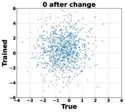
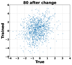
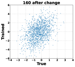
Figure 2: (Table) The mean computed values of $\eta_{t}$ pre and post-change with standard deviations in parentheses. (Plots) True vs. trained log-likelihood ratio evaluated on test samples at delay 0, 80, and 160 post-change. Computed by logistic-loss training of a fully-connected NN having 1 hidden layer on Gaussian sparse mean shift data in 100 dimensions.

Baselines.

The alternative baselines include (1) Exact CUSUM, (2) Window-limited CUSUM (WL-CUSUM), (3) Hotelling-CUSUM, (4) Multivariate Exponentially Weighted Moving Average (MEWMA), (5) Online Neural Network Classification (ONNC) and (6) Online Neural Network Regression (ONNR). Exact-CUSUM is included to provide a lower bound on EDDs for all the other baselines since it has full knowledge of the data distributions. More details are in Appendix B.

Calibration of procedure.

We can compare the baselines with NN-CUSUM under the standard metrics ARL and EDD introduced in Section 4.4. The direct computation of ARL is burdensome based on a large number of repetitions, each taking quite a long time to stop when there is no change. Now we provide an alternative to approximate the ARL with a much lower computation cost.

By borrowing the general arguments from [19, 20] and [17], the stopping time $\tau$ is asymptotically exponentially distributed for some rate parameter $\lambda$ relying on the threshold $b$

$$\mathbb{P}_{0}[\tau\leq c]-[1-\exp\{-\xi c\}]\to 0,\quad\mathbb{E}_{0}[\tau]\sim\xi^{-1}\quad\text{as}\quad b\to\infty,$$ (21)

where $\mathbb{P}_{0}[\cdot]$ is the probability measure under $f_{0}$. The argument that with no changes, all stopping times in this paper are asymptotically exponentially distributed can be advantageous. It allows for efficient simulation of the ARL without having to simulate the process until the stopping time $\tau$, which can be computationally expensive. Instead, one can simulate each sequence until a time $c$. Then an accurate estimate of $\mathbb{P}_{0}[\tau\leq c]$ can be obtained through the empirical frequency of the event $\{\tau\leq c\}$. The rate parameter $\xi$ can be solved with the cumulative distribution function of an exponential distribution equal to the estimate of $\mathbb{P}_{0}[\tau\leq m]$. An approximation of the ARL will be $\xi^{-1}$ as shown in (21).

Numerical Justification.

We first empirically verify that the NN training will produce a significant positive increment $\eta_{t}$ post-change (and around zero before change). The NN is trained on Gaussian sparse mean shift in $\mathbb{R}^{100}$ (more details in Appendix C) using logistic loss, and the NN is fully connected with 1 hidden layer of width 512. $w$ is the window length of the training and testing stacks, and training split portion $\alpha=0.5$. In the table in Figure 2, the positivity of post-change $\eta_{t}$ is obtained with $w=20$ and becomes more significant for larger window size. The distributions of $\eta_{t}$ pre- and post-change are shown in Figure A.1. As has been explained in Section 4.1, as long as $\eta_{t}$ gives a positive mean post-change the NN-CUSUM procedure can effectively detect the change point, which can happen with $w$ as small as 20 here. There is a trade-off in window size $w$ because larger $w$ may delay the detection though it gives a larger drift in $\eta_{t}$. The plot in Figure A.1 shows that the trained network function, though differs from the true $\log(f_{1}/f_{0})$, provides a certain approximation which is good enough to produce a positive $\eta_{t}$ post-change.

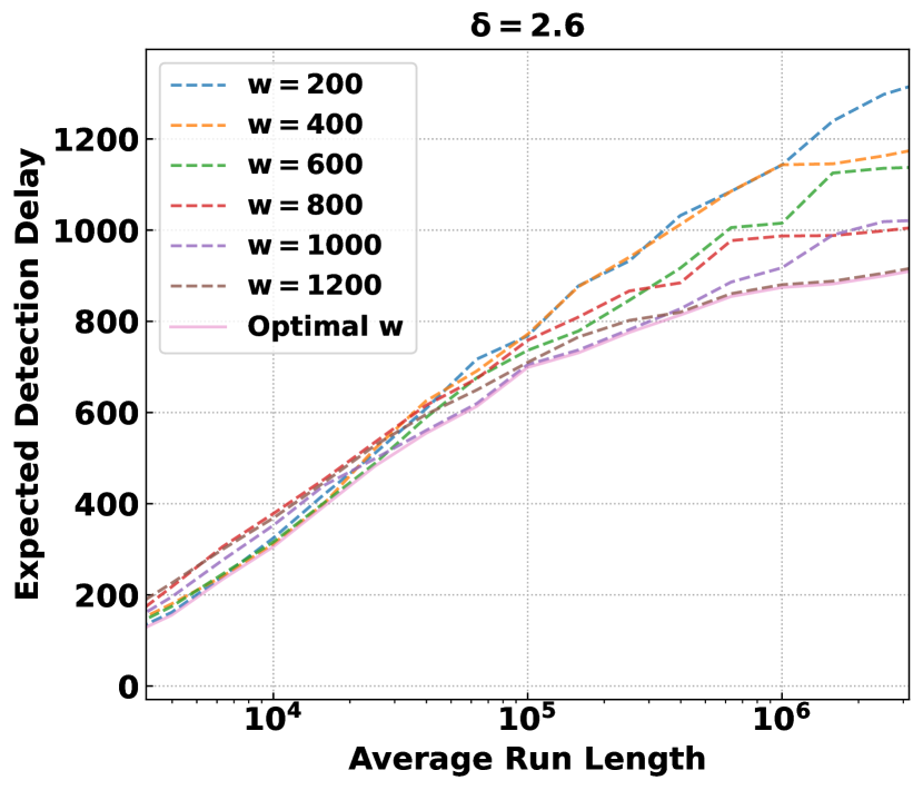
(a) Minimal EDD

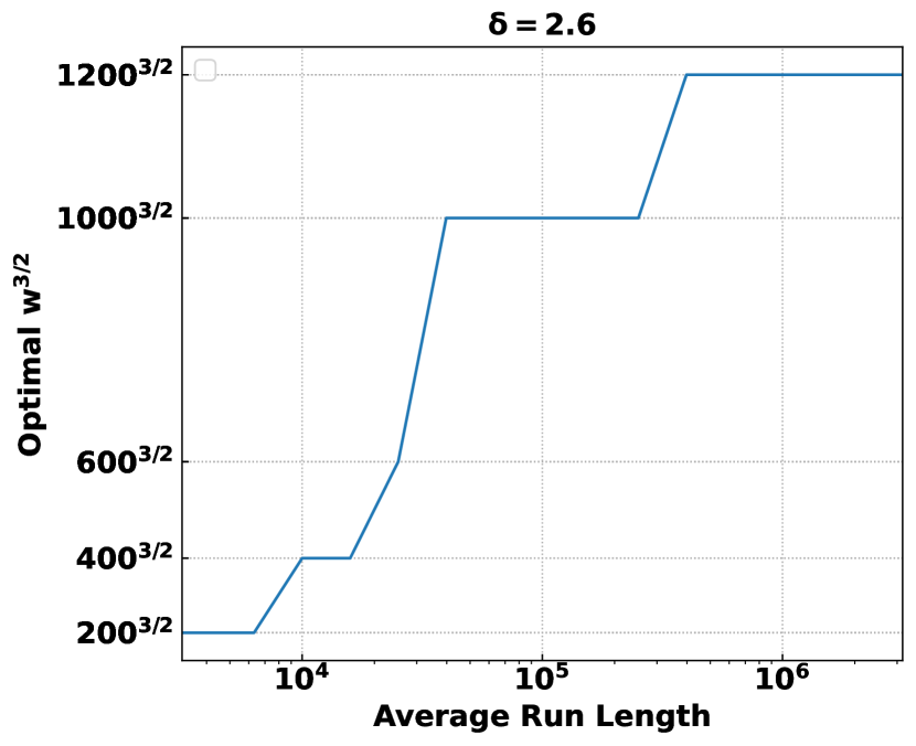
(b) Optimal window size $w$

Figure 3: (a) Minimal ARL vs EDD over window sizes from 200 to 1200 by 200; (b) Optimal window size $w$ vs ARL;

We further investigate the influence of window size $w$ on the ARL and EED. Figure 3 exhibits the numerical justification in the setting of the Gaussian mixture model with a component shift whose magnitude is $\delta=2.6$. The parameter $w$ varies from 200 to 1200, and $\alpha$ is between 0.1 and 0.8. In Figure 3(a), the dotted curves are the lowest EDD over all $\alpha$’s for every fixed $w$. And the lower envelope of EDDs is achieved by the optimal EDD over every pair of $w$ and $\alpha$. Over all $\alpha$’s, transitions of optimal $w$ can happen w.r.t. the growth of ARLs. Figure 3(b) indicates a linear relationship between the polynomial of $w$ and ARL. This is consistent with the theoretical relation suggested by the right hand side of (20).

Numerical Comparison.

We conduct extensive simulations throughout different settings on simulated high-dimensional data. Table 1 summarizes the numerical results under a fixed ARL at $5000$. Overall, NN-CUSUM outperforms other baselines in terms of smaller detection delays. In the Gaussian mean shift, WL-CUSUM is slightly better than NN-CUSUM since this setting is simple and the model mismatch in WL-CUSUM is avoided. In the Gaussian covariance shift, though WL-CUSUM still possesses appropriate parametric assumptions, the high dimension of data leads to a difficult estimation of the sample covariance and a large detection delay. NN-CUSUM is still one of the most competitive methods. In an average sense, MEWMA is better than NN-CUSUM. However, MEWMA also possesses high variance. For more complex data distributions like log Gaussian distributions and Gaussian mixture models, NN-CUSUM is consistently the most competitive one.

Table 1: For ARL$=5000$, EDDs on various methods and settings with data dimensions $100$. The standard deviations are reported in parentheses.

	Gaussian mean shift				Gaussian covariance shift
	$\delta=0.8$	$\delta=1.0$	$\delta=1.2$	$\delta=1.4$	$\rho=0.4$	$\rho=0.5$	$\rho=0.6$	$\rho=0.7$
NN-CUSUM	$508.00{(58.643)}$	$399.70{(28.853)}$	$353.80{(22.868)}$	$343.00{(16.371)}$	$988.80{(180.737)}$	$877.50{(124.783)}$	$718.10{(67.839)}$	$632.40{(65.882)}$
ONNC	$1808.35{(504.784)}$	$810.50{(412.678)}$	$721.88{(301.904)}$	$872.17{(101.257)}$	$1211.30{(165.680)}$	$1022.46{(118.554)}$	$955.78{(90.635)}$	$882.90{(55.607)}$
ONNR	$1059.67{(645.337)}$	$1258.66{(266.482)}$	$989.78{(157.136)}$	$617.80{(246.583)}$	$1460.10{(794.503)}$	$1169.06{(606.176)}$	$1096.34{(410.372)}$	$892.71{(362.830)}$
WL-CUSUM	$521.51{(48.580)}$	$362.56{(27.294)}$	$271.21{(19.096)}$	$208.93{(15.152)}$	$3325.83{(39.851)}$	$2931.66{(35.324)}$	$2581.79{(36.266)}$	$2341.10{(42.671)}$
MEWMA	$1196.44{(1149.512)}$	$482.66{(380.023)}$	$282.27{(274.986)}$	$162.93{(149.694)}$	$856.38{(910.125)}$	$512.58{(485.139)}$	$333.89{(368.357)}$	$220.55{(213.151)}$
Hotelling-CUSUM	$927.99{(419.346)}$	$735.55{(295.524)}$	$508.18{(136.690)}$	$358.79{(92.238)}$	$2895.87{(1524.820)}$	$3273.19{(1544.348)}$	$3098.57{(1582.602)}$	$2486.91{(1582.011)}$
Exact-CUSUM	$13.57{(6.304)}$	$9.10{(4.826)}$	$7.26{(4.194)}$	$4.90{(2.914)}$	$4.79{(2.906)}$	$2.96{(2.332)}$	$1.99{(1.375)}$	$1.41{(1.001)}$

	Log Gaussian covariance shift				Gaussian mixture model with component shift
	$\rho=0.5$	$\rho=0.6$	$\rho=0.7$	$\rho=0.8$	$\delta=2.6$	$\delta=2.8$	$\delta=3.0$	$\delta=3.2$
NN-CUSUM	$809.50{(122.330)}$	$649.50{(96.906)}$	$656.40{(90.572)}$	$579.60{(58.426)}$	$501.50{(238.384)}$	$489.00{(184.732)}$	$436.40{(139.926)}$	$439.40{(104.086)}$
ONNC	$898.80{(81.565)}$	$824.26{(73.915)}$	$751.82{(49.054)}$	$738.58{(48.261)}$	$748.16{(766.567)}$	$455.44{(340.327)}$	$698.50{(597.975)}$	$552.96{(526.050)}$
ONNR	$741.41{(774.347)}$	$996.78{(925.933)}$	$664.29{(423.954)}$	$641.46{(433.003)}$	$1824.24{(1199.535)}$	$1350.01{(837.241)}$	$1364.20{(733.951)}$	$1234.14{(684.074)}$
WL-CUSUM	$4786.62{(73.538)}$	$4721.39{(89.170)}$	$4694.93{(97.554)}$	$4598.74{(90.818)}$	$4699.42{(37.399)}$	$4671.49{(38.534)}$	$4635.17{(36.026)}$	$4610.90{(41.614)}$
MEWMA	$2607.87{(1746.947)}$	$1429.36{(1091.883)}$	$1066.95{(1037.376)}$	$1036.82{(934.255)}$	$3883.60{(1564.703)}$	$4343.19{(1349.269)}$	$4175.54{(1467.160)}$	$4076.63{(1471.006)}$
Hotelling-CUSUM	$2823.57{(1692.267)}$	$2630.29{(1634.382)}$	$2446.73{(1625.028)}$	$2178.87{(1507.793)}$	$5000.00{(0.000)}$	$5000.00{(0.000)}$	$5000.00{(0.000)}$	$5000.00{(0.000)}$
Exact-CUSUM	$1.43{(1.259)}$	$0.95{(0.942)}$	$0.61{(0.811)}$	$1.00{(0.000)}$	$3.64{(3.738)}$	$2.35{(2.471)}$	$2.54{(2.931)}$	$2.20{(2.462)}$

6 Real Data Experiments

We evaluated NN-CUSUM and baselines on two tasks using real-world data: human activity detection and Higgs boson detection. and Higgs Boson detection [21]. Details of each dataset are available in Appendix D. Since the asymptotic estimation of ARL (21) is not available for real-world data, we computed EDD by averaging the detection delay of multiple sequences of data on a chosen threshold for a specific rate of type-I error. Details of the setup for each experiment are available in Appendix E. We also conducted additional experiments to explore the impact of hyperparameters on performance. The results of additional experiments are available in Appendix F.

Human activity change detection.

For the human activity change detection task, we use Human Activity Sensing Consortium (HASC) 2013 challenge dataset [22]. The dataset consists of 3-dimensional G-force measurements of several human activities. We selected four activities from the dataset (walk, jog, skip, and stair up) to construct four ordered activity sequence pairs for evaluation. A change-point detection method is expected to detect the time index when the activity change. Table 2 shows EDD of NN-CUSUM and baselines for the activity pairs on the threshold chosen by 0.05 type-I error. We observe that Hotelling-CUSUM, WL-CUSUM, and MEWMA show better performance in the case where there exists a significant difference in the two activities. In those cases, while NN-CUSUM does not always outperform other baselines NN-CUSUM shows consistent performance with lower standard deviations. Hotelling-CUSUM, WL-CUSUM, and MEWMA achieve unstable detection performance in the cases where the difference in two activities is not obvious, showing failures in detection. NN-CUSUM achieves consistent performance outperforming or showing comparable performance with other baselines.

Table 2: Expected detection delay of NN-CUSUM and baselines on human activity detection. The threshold was chosen by 0.05 type-I error. * denotes the result includes at least one failure in detection. - denotes complete failure in detection. The standard deviation was reported in parentheses.

	NN-CUSUM	ONNC	ONNR	Hotelling-CUSUM	WL-CUSUM	MEWMA
Walk$\rightarrow$Stairup	$291.4{(36.5)}$	$292.3{(146.8)}$	$242.6{(136.5)}$	$666.9^{\ast}{(327.8)}$	$147.5^{\ast}{(287.7)}$	$533.8^{\ast}{(467.8)}$
Jog$\rightarrow$Skip	$209.6{(30.6)}$	$222.3{(83.8)}$	$170.0{(77.1)}$	$49.9{(30.1)}$	$57.0{(47.6)}$	$27.9{(23.0)}$
Skip$\rightarrow$Jog	$281.6{(50.0)}$	$315.8{(95.5)}$	$367.1{(81.9)}$	-	$101.8{(42.5)}$	-
Stairup$\rightarrow$Walk	$371.4{(71.0)}$	$477.7{(166.8)}$	$347.0{(127.7)}$	$387.0^{\ast}{(330.5)}$	$627.2^{\ast}{(380.9)}$	$586.7^{\ast}{(425.6)}$

Higgs boson detection.

We use Higgs dataset from the University of California Irvine machine learning repository [23]. The Higgs dataset contains 28 features extracted from two types of signal: one that produces Higgs bosons that occur only at extremely high-energy densities; and a background signal that does not produce Higgs bosons [21]. For the Higgs boson detection task, we construct sequences where post-change data are the features of the Higgs boson produced signal and pre-change data are the features of the background signal. We expect a change-point detection method to detect the time index when the data changes from the background signal to the Higgs boson produced signal. Table 3 shows the EDD of NN-CUSUM and baselines on Higgs boson detection. NN-CUSUM outperforms all other baselines. ONNR and Hotelling-CUSUM include at least one failure to detect change-point over multiple sequences. MEWMA completely fails to detect change-point.

Table 3: Same baselines as in Table 2 for Higgs boson detection.

NN-CUSUM	ONNC	ONNR	Hotelling-CUSUM	WL-CUSUM	MEWMA
$425.5{(96.1)}$	$440.1{(98.9)}$	$722.5^{\ast}{(292.3)}$	$965.9^{\ast}{(111.7)}$	$497.8{(18.3)}$	-

7 Discussion

We present a new framework for online change-point detection, which we call neural network CUSUM (NN-CUSUM). The motivation is that the training of a logistic loss will converge (in population) to a log-likelihood ratio between two samples, which thus naturally motivated us to construct CUSUM statistics using the sequentially learned neural network to test samples. We developed a novel online procedure by training and testing data-splitting to achieve online change-point detection. The new procedure is compared with Hotelling-CUSUM to show its good performance on simulated and real data experiments. The performance gain is particularly large for high-dimensional data.

The approach can be extended in several directions. Ongoing work includes establishing theoretical performance property guarantees by combining the training dynamic of neural networks with analysis of change-point detection procedures, and hopefully to show the near optimality since the detection statistic is based on approximating the log-likelihood ratio based CUSUM.

Appendix A Proofs

Proof of Lemma 4.1.

Let $g={\hat{\theta}}$ be fixed, $\sup_{x\in\mathcal{X}}|g(x)|\leq C$. By definition, with $m^{\prime}=(1-\alpha)w$,

$$\eta_{t}=\frac{1}{m^{\prime}}\sum_{i=1}^{m^{\prime}}(g(x_{i})-g(\tilde{x}_{i})),$$

where $x_{i}\sim f_{1}$, i.i.d,. $\tilde{x}_{i}\sim f_{0}$, i.i.d., and are independent. The the random variable $(g(x_{i})-g(\tilde{x}_{i}))$ is i.i.d. and is bounded by $2C$. The lemma directly follows Classical Hoeffding’s inequality. ∎

Proof of Lemma 4.2.

The proof follows a similar argument in [14, Lemma B.1]. By definition (15),

$$\bar{\eta}:=\mathbb{E}_{1}[\eta_{t}^{\rm NTK}|D_{t}^{\rm tr}]=\int(\phi_{1}(x^{\prime})-\phi_{0}(x^{\prime}))(\hat{f}_{1,t}^{\rm tr}(x^{\prime})-\hat{f}_{0,t}^{\rm tr}(x^{\prime}))dx^{\prime},$$

where

$$\phi_{i}(x^{\prime}):=\int K_{0}(x,x^{\prime})f_{i}(x)dx,\quad i=0,1.$$

Thus $\bar{\eta}$ can be written as the independent sum over the training samples as

$$\bar{\eta}=\frac{1}{m}\sum_{i=1}^{m}(\phi(x_{i})-\phi(\tilde{x}_{i})),\quad\phi:=\phi_{1}-\phi_{0},$$

where $x_{i}\sim f_{1}$, i.i.d,. $\tilde{x}_{i}\sim f_{0}$, i.i.d. are from the training split and are independent, $m=\alpha w$. Meanwhile, by the uniform boundedness of $K_{0}(x,x^{\prime})\in[0,B]$,

$$\phi_{i}(x)\in[0,B],\quad\forall x\in\mathcal{X},\quad i=0,1.$$

As a result,

$$|\phi(x)|=|\phi_{1}(x)-\phi_{0}(x)|\leq B,\quad\forall x\in\mathcal{X}.$$

Then, the classical Hoeffding inequality gives that for any $\lambda>0$,

$$\mathbb{P}_{1}[\bar{\eta}-\mathbb{E}_{1}\bar{\eta}<-\lambda B\sqrt{\frac{1}{\alpha w}}]\leq e^{-\lambda^{2}/2},$$

where the probability $\mathbb{P}_{1}$ is over the randomness of the training data $D_{t}^{\rm tr}$ post change. Recall that $\mathbb{E}_{1}\bar{\eta}=\eta^{*}$ by definition, the lemma follows by taking $\lambda=\sqrt{2\log(1/\delta)}>0$. ∎

Appendix B Experimental Baselines

In this section, we introduce the technical details on the compared baselines. As a general scheme for change-point detection, the practitioners need to calculate the statistics at each time and compare the statistics with a pre-specified threshold. When the sequential statistics exceed a threshold at some time $t$, an alarm will be raised to claim a change happens and the stopping time $\tau$ will be set to the value $t$.

Window-Limited CUSUM (WL-CUSUM) procedure.

WL-CUSUM is extensively designed in [24]. When the pre-change density $f_{0}$ is fully known and the post-change density $f_{1}(\cdot,\theta)$ possesses a known form but an unknown parameter $\theta\in\Theta$, the log-likelihood ratio is adjusted adaptively as:

$$\ell(x_{t},\hat{\theta}_{t-1})=\log\frac{f_{1}(x_{t},\hat{\theta}_{t-1})}{f_{0}(x_{t})},$$

where $\hat{\theta}_{t-1}\in\Theta$ is an estimation of $\theta$. If a window size $w$ is fixed, the estimation $\hat{\theta}_{t}$ relies on the data within the window $\{x_{t},\ldots,x_{t-w+1}\}$. The option on the estimator is not rigid. The most common option could be the Maximum Likelihood Estimator (MLE) taking the form:

$$\hat{\theta}_{t}=\operatorname*{arg\,max}_{\theta\in\Theta}\sum_{i=0}^{w-1}\log f_{1}\left(x_{t-i},\theta\right),$$

which we will adopt throughout the experiments. The remaining would be similar to the exact CUSUM. With $S_{0}^{\rm WLC}=0$, the recursion takes the form:

$$S_{t}^{\rm WLC}=(S_{t-1}^{\rm WLC}+\ell(x_{t},\hat{\theta}_{t-1}))^{+}.$$

And the stopping time is determined by:

$$\tau_{\rm WLC}=\inf\{t:S_{t}^{\rm WLC}>b\},$$

with the threshold $b$.

Hotelling CUSUM procedure.

Instead of using the exact log-likelihood ratio in the recursion, the Hotelling CUSUM procedure (motivated by the classic Hotelling T-square statistics) uses the Hotelling T-square statistic in the recursion. It can be treated as a non-parametric detection statistic (only uses the first and the second order moments). It is good in detecting mean shifts but not very effective in detecting other types of changes (such as covariance shifts). Define

$$\begin{split}g_{0}^{\rm H}(x_{t})&:=\frac{1}{2}(x_{t}-\hat{\mu}_{p})^{T}(\widehat{\Sigma}_{p}+\lambda I_{d})^{-1}(x_{t}-\hat{\mu}_{p}),\\ g^{\rm H}(x_{t})&:=g_{0}^{\rm H}(x_{t})-\hat{d}_{p}\end{split}$$

where $\hat{\mu}_{p}$ and $\widehat{\Sigma}_{p}$ are estimated mean, and covariance matrix from the pilot sequence assumed to be drawn from $f_{0}$; $\hat{d}_{p}$ usually set to be $\mathbb{E}_{x\sim f_{0}}g^{\rm H}_{0}(x)+\epsilon$ for some small constant $\epsilon$ and is computed by sample average on a test split of the pilot sequence in practice. The positive scalar $\lambda$ is a regularizing parameter because the covariance matrix estimator $\widehat{\Sigma}_{p}$ may be singular, e.g., when the data dimension is high compared to the size of the pilot sequence. Once $\hat{\mu}_{p}$, $\widehat{\Sigma}_{p}$ and $\hat{d}_{p}$ are pre-computed on the pilot set, the recursive CUSUM is computed upon the arrival of stream samples of $x_{t}$ as

$$S^{\rm H}_{t}=(S^{\rm H}_{t-1}+g^{\rm H}(x_{t}))^{+}.$$

The associated stopping time procedure is $\tau_{H}=\inf\{t:S^{\rm H}_{t}>b_{\rm H}\}$.

Multivariate Exponentially Weighted Moving Average (MEWMA).

The MEWMA procedure is a statistical method commonly used in quality control and process monitoring. It is designed to detect shifts or abnormalities in multivariate data by analyzing the mean vector and covariance structure. MEWMA calculates a statistic that combines the differences between the current observation and the expected values based on historical data, weighted by exponentially decreasing weights. This weighting scheme assigns more importance to recent observations while still considering the entire history. By comparing the calculated statistic to control limits, the MEWMA procedure can identify when a process is out of control and signal the need for investigation or corrective action. As was introduced in [25], MEWMA computes

$$z_{t}=rx_{t}+(1-r)z_{t-1},\quad t\geq 1$$

where $z_{0}=0$ and the decay rate belongs to the range $0<r\leq 1$. The MEWMA chart raises the alarm under the stopping time

$$\tau_{\rm M}=\inf\{t:z_{t}^{\top}\Sigma_{z_{t}}^{-1}z_{t}>b_{\rm M}\}$$

where the covariance matrix of $z_{t}$ yields the closed form $\Sigma_{z_{t}}=\left(r\left(1-(1-r)^{2t}\right)/(2-r)\right)\Sigma_{0}$ and $b_{\rm M}$ is a mannualy selected threshold.

Online Neural Network Classification (ONNC).

ONNC is an online change-point detection algorithm based on neural networks proposed in [13]. It processes mini-batches of time series observations sequentially and estimates whether they have the same distribution or not. The algorithm compares two mini-batches of observations using a neural network and calculates a distance metric between them. If the distance exceeds a certain threshold, it signals a change point. The implementation is encoded in the Algorithm 1 in [13].

Online Neural Network Regression (ONNR).

ONNR is another neural network-based online change-point detection algorithm introduced in [13]. Similar to ONNC, it processes mini-batches of time series observations sequentially and compares them using a dynamically training neural network. The difference between ONNR from ONNC is that instead of calculating a distance metric between mini-batches, ONNR predicts the next observation in each mini-batch and compares the prediction errors. If the prediction errors exceed a certain threshold, an alarm will be raised. The details are revealed in Algorithm 2 in [13].

Appendix C Additional Simulations

Throughout the simulated experiments, we generate the sequences with a total length $10,000$ and the change point located in the middle, namely $k=5,000$. To compute stable performance metrics, we generate $100$ sequences to perform the detection procedures under each setting. Meanwhile, all methods share pilot data containing $100$ pre-change sequences with lengths $10,000$. The detection procedures are allowed to learn the statistical behavior of the pre-change process from the pilot data.

The neural network architecture of NN-CUSUM consists of one fully-connected hidden layer with ReLU activation. We set the dimension of the hidden layer to 512. The last layer is a one-dimensional fully-connected layer without activation. The training batch size was set to 10 with 5 epochs. The stride of the sliding window and the number of training/testing stacks were set to 10 and 100 respectively. We used Adam [15] for training.

C.1 Numerical Justification

We introduce additional numerical justifications within the setting of the Gaussian sparse mean shift. Figure A.1 is a visualization of the table in Figure 2. The data is generated as a sequence with a length 20000 and dimensions 100. The mean shift happens at the time 10000. The neural network is dynamically trained along the sequence under with the logistic error function. During this procedure, the empirical distribution of the increments $\eta_{t}$’s is visualized under different window size $w$. Figure A.1 supports the table more intuitively by a tendency that as the sizes of training and testing windows both increase, the shift in the mean of $\eta_{t}$ becomes more evident, potentially representing a faster detection.

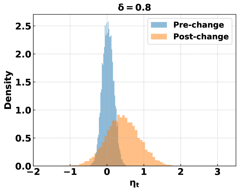
(a) $w=20$.

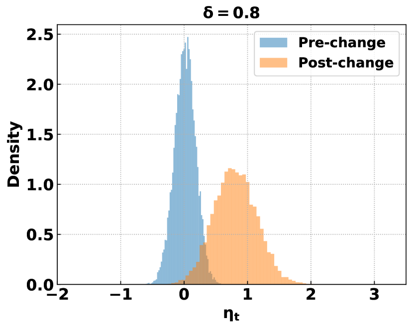
(b) $w=60$.

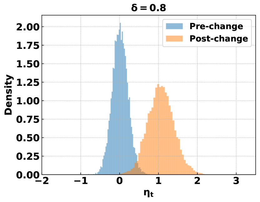
(c) $w=100$.

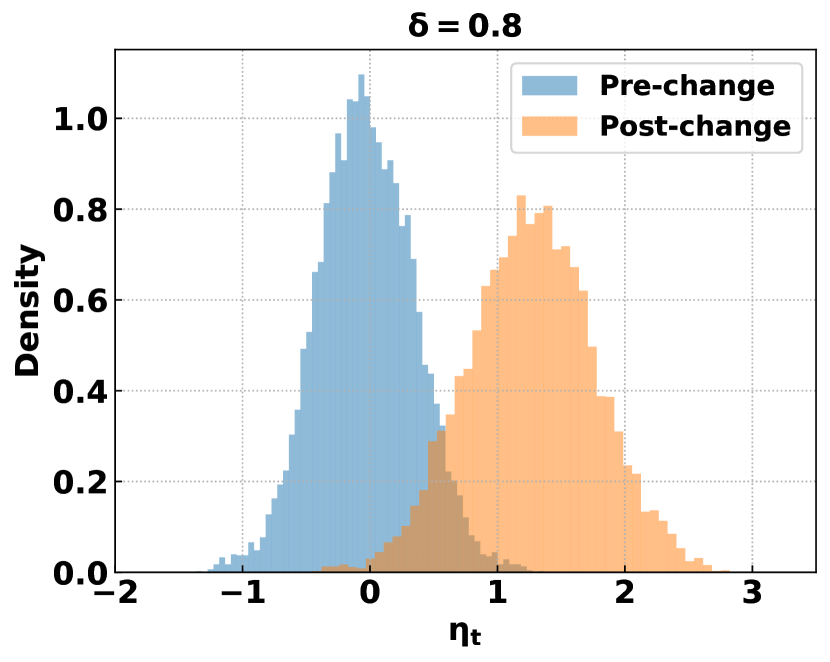
(d) $w=200$.

Figure A.1: Distribution of $\eta_{t}$ pre and post-change.

Figure A.2 demonstrates the training convergence of the separate training on pre and post-change sequences of the neural networks. Multiple sequences are plotted simultaneously. The figure serves as a sanity check to validate the stable convergence of the neural network in the proposed scheme.

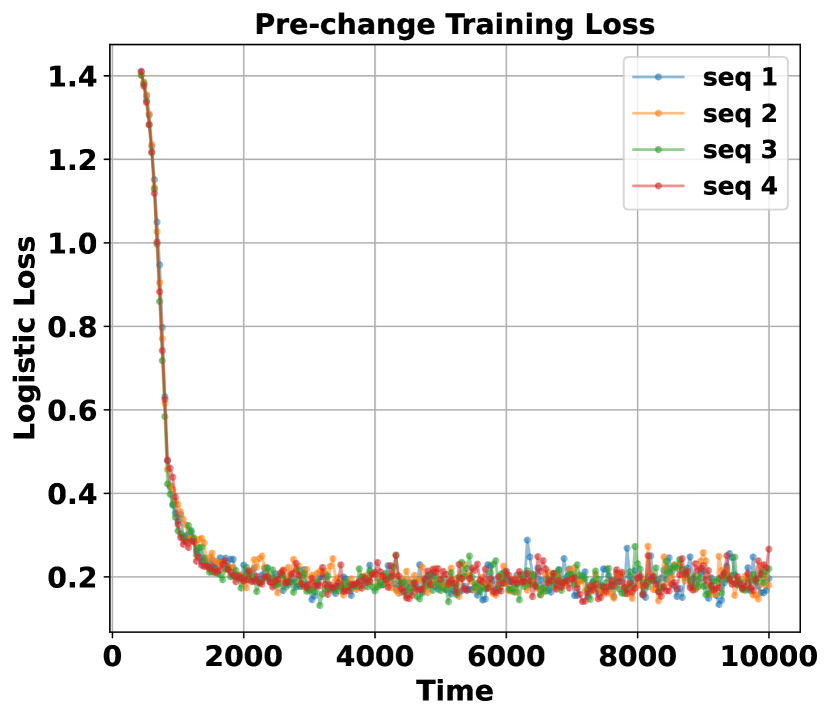
(a) Pre-change training logistic loss

(b) Post-change training logistic loss

Figure A.2: (a) Convergence of pre-change training logistic loss over time; (b) Convergence of post-change training logistic loss over time.

C.2 Numerical Comparison

Gaussian Distribution with Sparse Mean Shift.

In this experiment, we evaluate the methods on 100-dimensional vector data from Gaussian distribution with sparse mean shifts. To be precise, for the fixed dimension $d=100$, the pre-change distribution $f_{0}$ is $\mathcal{N}(0,I_{d})$ and post-change distribution $f_{1}$ is $\mathcal{N}(\mu_{q},I_{d})$ with the shifted mean vector $\mu_{q}=(\delta,\delta/2,\delta/3,0,\cdots,0)^{T}$ and a pre-specified mean shift magnitude parameter $\delta\in\{0.8,1,1.2,1.4\}$. This is a challenging case since the post-change mean vector is sparse.

Figure A.3 presents a log ARL-EDD plot for sparse mean shift experiments. NN-CUSUM and WL-CUSUM demonstrate competitive performance in achieving the lowest EDD in different ARL ranges when the mean shift magnitude is not large ($\delta\in\{0.8,1.0,1.2\}$). Hotelling-CUSUM and MEWMA charts exhibit slow detection of the sparse and non-significant mean shift, with their delays increasing significantly with larger ARL. For relatively significant magnitudes ($\delta=1.4$), WL-CUSUM charts outperform the other baselines. Overall, in mild shift magnitudes, NN-CUSUM shows highly competitive performance and Hotelling-CUSUM and MEWMA take thousands of steps more than NN-CUSUM and WL-CUSUM to detect the change. Once the magnitude is evident, NN-CUSUM remains comparable with the others, with a detection difference of less than 500 steps.

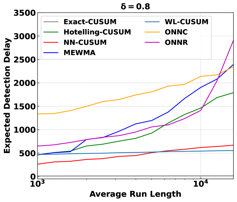
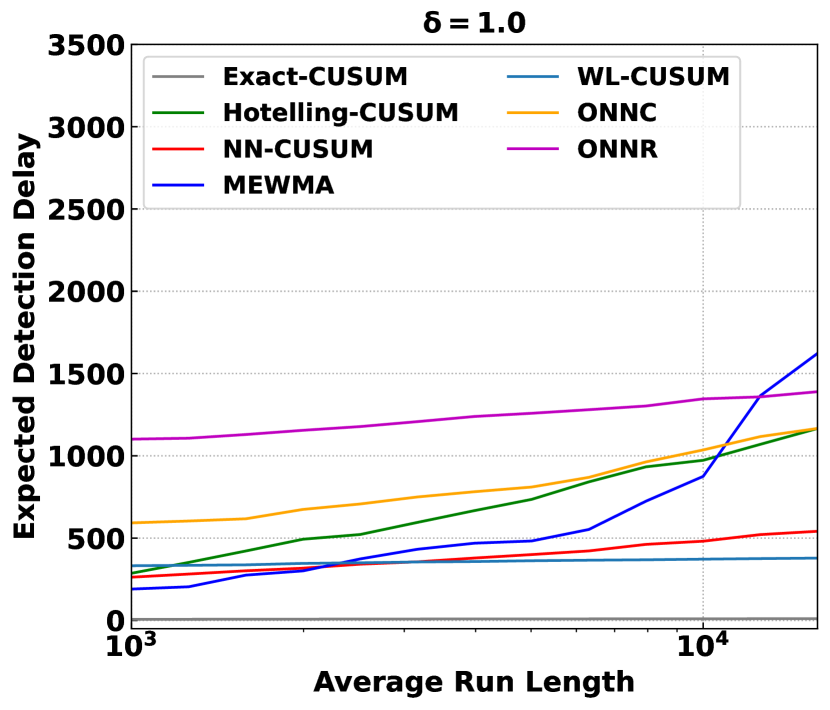
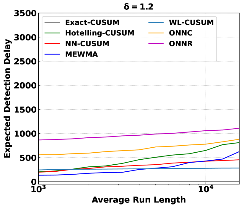
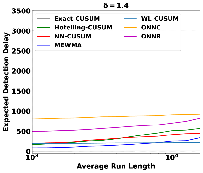
Figure A.3: EDD v.s. ARL on 100-dimensional Gaussian distributed data with a sparse mean shift varying its magnitude $\delta$ in $\{0.8,1.0,1.2,1.4\}$.

Gaussian Distribution with Sparse Covariance Shift.

We are also interested in the detection of the sparse covariance shift. Still, we fix the dimension $d=100$. The pre-change distribution $f_{0}$ is $\mathcal{N}(0,I_{d})$ and post-change distribution $f_{1}$ is $\mathcal{N}\mbox{$\left({0,I_{d}-D^{2}+DED}\right)$}$, where $E$ is $d\times d$ all-ones matrix and $D$ is a specified diagonal matrix. To be precise, we have $D=\sqrt{\rho}D_{0}$ where $D_{0}$ is a sparse diagonal matrix with 10 out of 100 of the diagonal entries being ones and the remaining entries being zeros. The index set of non-zero diagonal entries is specified as $\{1,11,\ldots,81,91\}$. The covariance shift magnitude $\rho$ varies in $\{0.4,0.5,0.6,0.7\}$. Such a design of $D$ triggers quite sparse non-zero covariances between the coordinates.

The log ARL-EDD plot in Figure A.4 depicts the performance of different methods in sparse covariance shift experiments. With small magnitudes of the shift ($\rho=0.4,0.5$), NN-CUSUM outperforms other methods by achieving the smallest EDDs at any given ARL. Meanwhile, the baseline MEWMA can accomplish the detection task relatively well. When $\rho=0.6,0.7$, NN-CUSUM and MEWMA show comparably quick detection ability. In contrast, the Hotelling-CUSUM charts exhibit rapid deterioration in performance as the ARL grows, indicating that it is ill-suited for high-dimensional sparse covariance detection. The WL-CUSUM shows stable EDD w.r.t. the varying ARL. However, WL-CUSUM also has evident disadvantages compared to NN-CUSUM and MEWMA. Notably, as the magnitude of the shift increases, most of the methods exhibit a decrease in detection delay, serving as a sanity check for the performance of these methods.

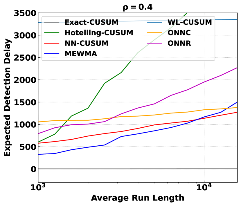
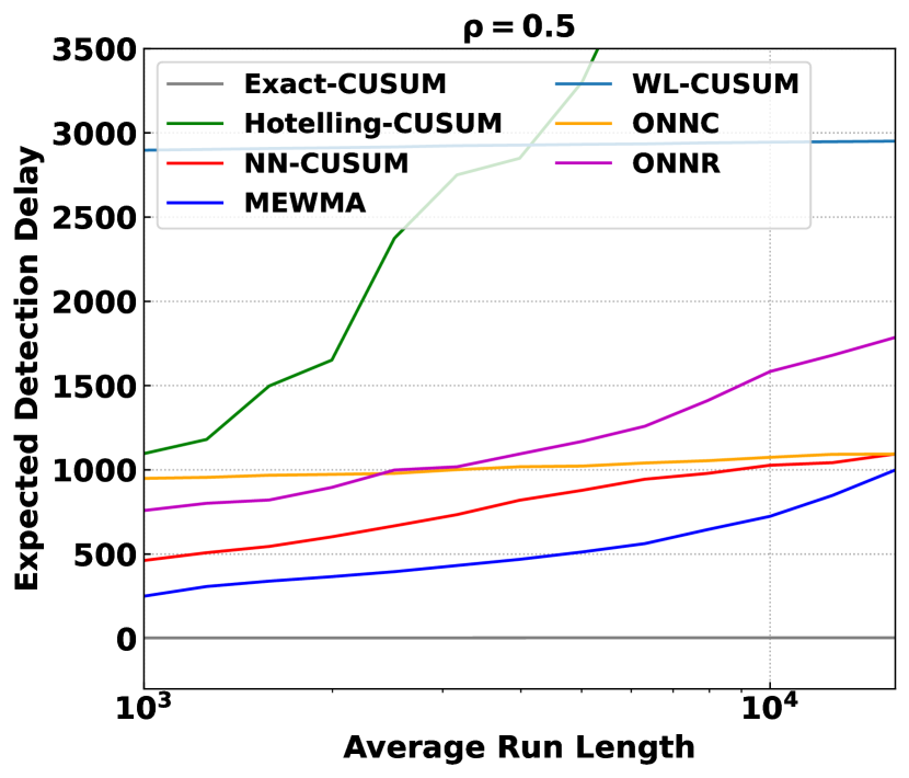
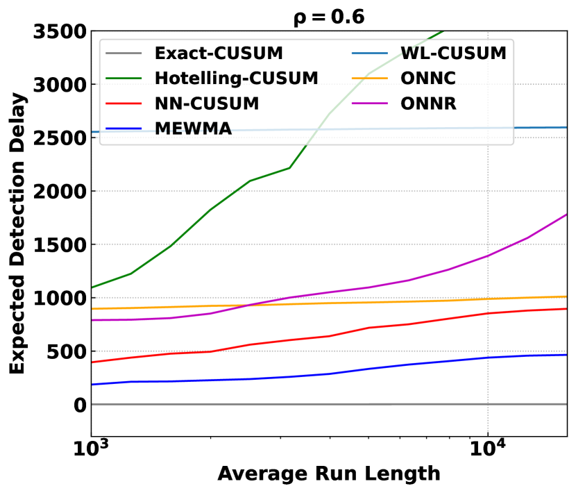
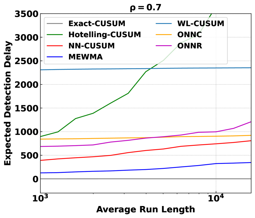
Figure A.4: EDD v.s. ARL on 100-dimensional Gaussian distributed data with a sparse covariance shift varying its magnitude $\rho$ in $\{0.4,0.5,0.6,0.7\}$.

Log Gaussian Distribution with Sparse Covariance Shift.

We also the detection of the sparse covariance shift for non-normal distribution. With data dimension $d=100$, we generate data following log-normal distribution. To be precise, the pre-change distribution $f_{0}$ is $\exp\{\mathcal{N}(0,I_{d})\}$ and post-change distribution $f_{1}$ is $\exp\{\mathcal{N}\mbox{$\left({0,I_{d}-D^{2}+DED}\right)$}\}$, where $E$ is all-ones matrix. $D$ is defined similarly as in the sparse diagonal matrix case with 20 out of 100 diagonal entries being ones. The covariance shift magnitude $\rho$ varies in $\{0.5,0.6,0.7,0.8\}$. Figure A.5 demonstrates that NN-CUSUM and ONNC are the most acute in detection of the sparse covariance shift in high-dimensional log-normal distribution. Hotelling-CUSUM, MEWMA and ONNR gradually lose their efficiency to detect the change as the ARL grows large. WL-CUSUM adopts the parametric form for the shift in Gaussian distributions. Thus the skewness in log Gaussian distribution leads to its failure.

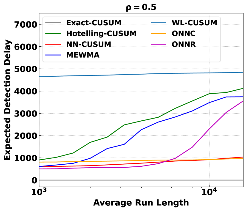
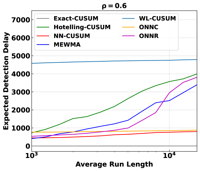
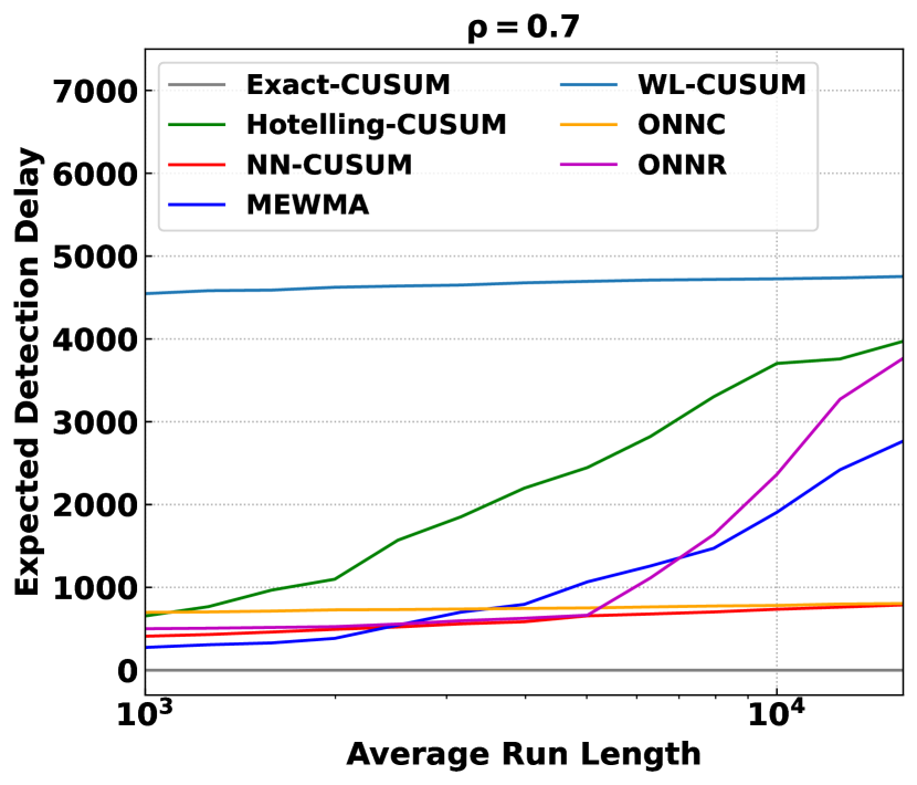
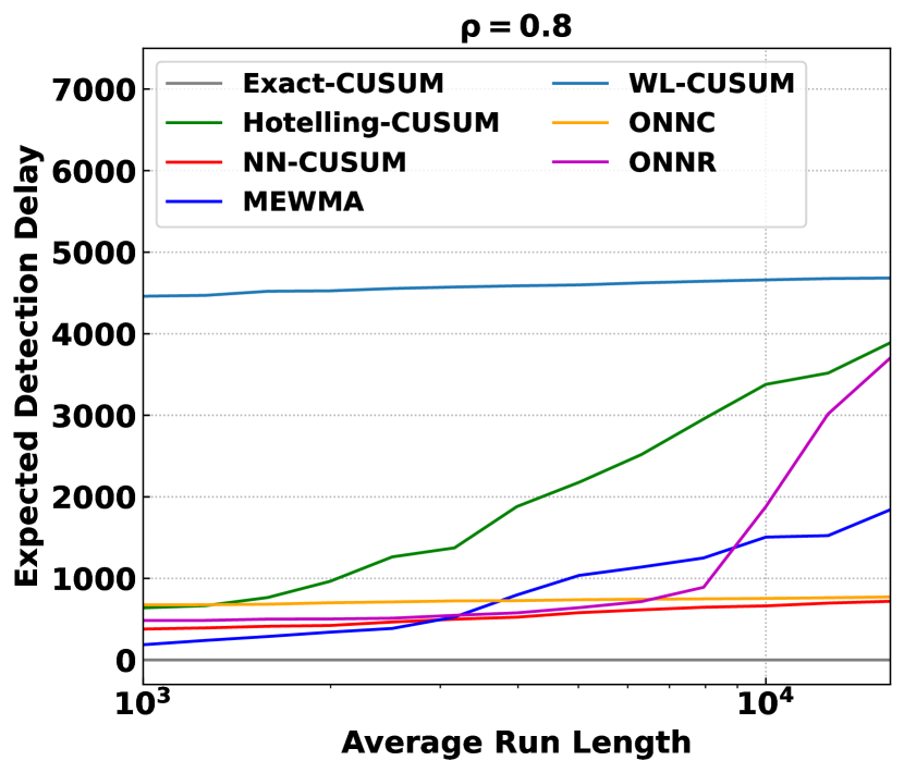
Figure A.5: EDD v.s. ARL on 100-dimensional Log Gaussian distributed data with a sparse covariance shift varying its magnitude $\rho$ in $\{0.5,0.6,0.7,0.8\}$.

Gaussian Mixture Model with Component Shift.

Besides the conventional shift types, namely the mean shift and covariance shift, we also design Gaussian mixture model with component shift to mimic the complex dynamics in real data. With $d=100$, the pre-change distribution $f_{0}$ is $\frac{1}{2}\mathcal{N}(2e_{d},I_{d})+\frac{1}{2}\mathcal{N}(-2e_{d},I_{d})$ and post-change distribution $f_{1}$ is $\frac{1}{3}\mathcal{N}\mbox{$\left({2e_{d},I_{d}}\right)$}+\frac{1}{3}\mathcal{N}\mbox{$\left({-2e_{d},I_{d}}\right)$}+\frac{1}{3}\mathcal{N}\mbox{$\left({\delta e_{d},(1-\rho)I_{d}+\rho E}\right)$}$ where the $d$-dimensional vector $e_{d}$ is an all-one vector and the $d\times d$ matrix $E$ is an all-one matrix. The mean shift magnitude $\delta$ varies in $\{2.6,2.8,3.0,3.2\}$ and the covariance shift magnitude $\rho$ is fixed at $0.2$.

Figure A.6 exhibits the performance of each method in the detection of Gaussian mixture component shift. NN-CUSUM steadily outperforms each method with considerably lower EDD at a relatively large ARL level. NN-CUSUM is the most competitive method in complex data shifts. Non-parametric methods are better than the methods based on certain parametric assumptions. For parametric methods, faced with complex data shifts, violations of their assumptions or model mismatch could cause the failure of detection.

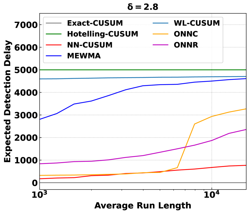
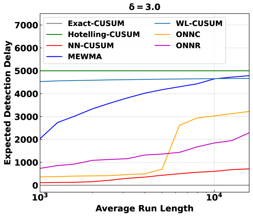
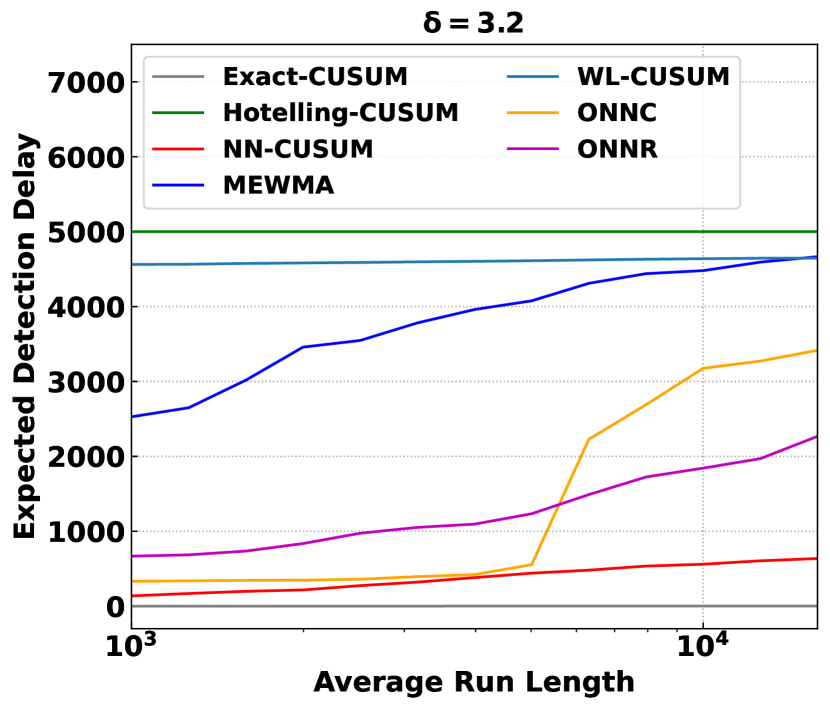
Figure A.6: EDD v.s. ARL on 100-dimensional Gaussian Mixture model data with a component shift varying its mean shift magnitude $\delta$ in $\{2.6,2.8,3.0,3.2\}$.

Varying Dimensions.

To study the impact of the data dimensions on the detection, we let the dimension of data varies in $\{2,5,10,20\}$ in the Gaussian mixture component shift dataset. We select the case $\delta=2.8$, which is the most manifest to detect.

Figure A.7 demonstrates the impact of dimensionality on the detection performance of different methods. Despite the complexity of the data shift structure, both Hotelling-CUSUM and WL-CUSUM exhibit effective detection performance when the dimension is low. However, as the dimension increases, the performance of Hotelling-CUSUM experiences a sharp decline, while WL-CUSUM exhibits relatively better resilience. Nonetheless, even WL-CUSUM exhibits manifest deterioration in performance as the dimension reaches 20. In contrast, NN-CUSUM maintains robust and satisfactory detection ability throughout the process, with an EDD consistently lower than 1,000.

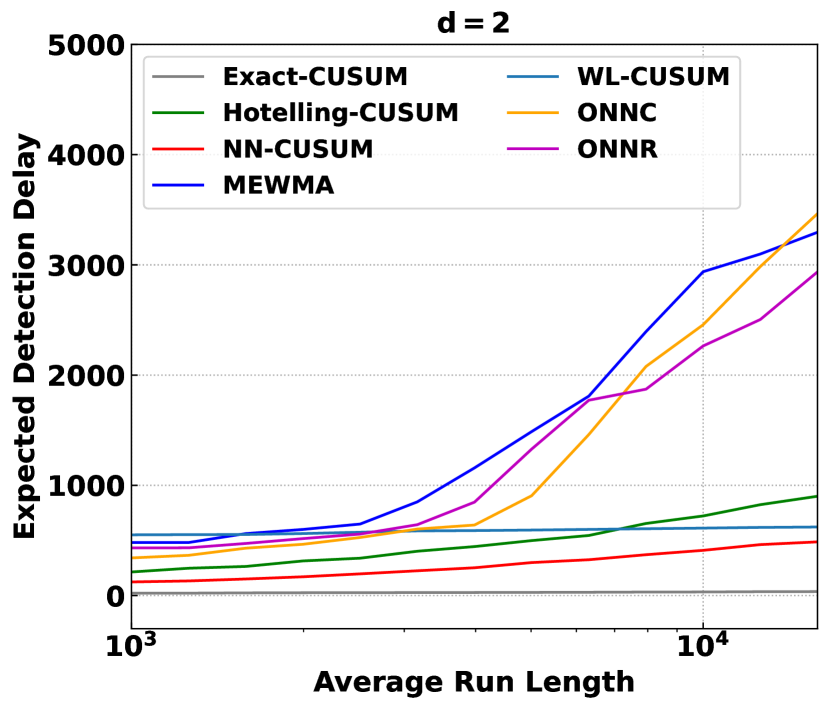
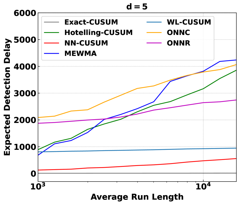
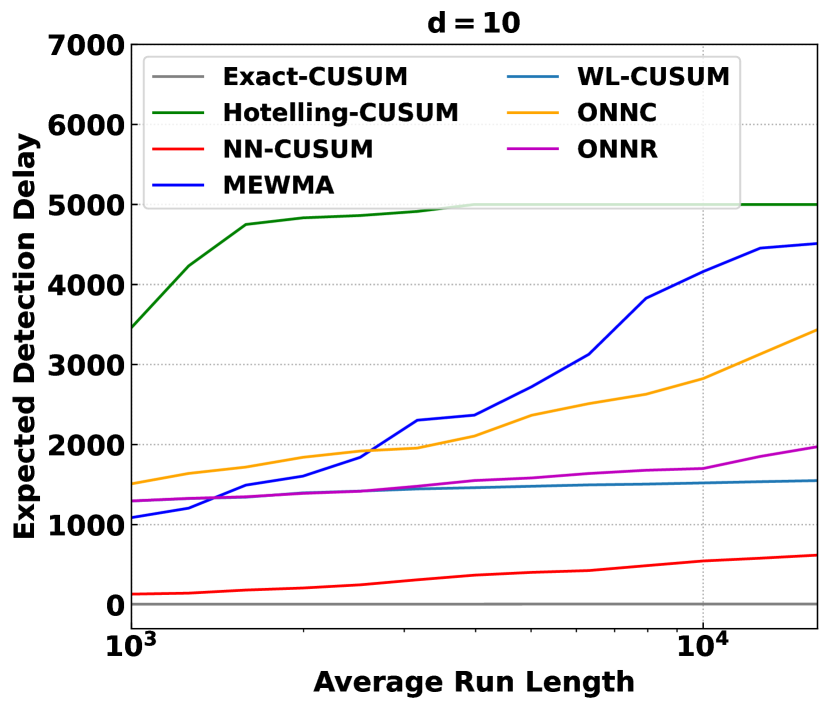
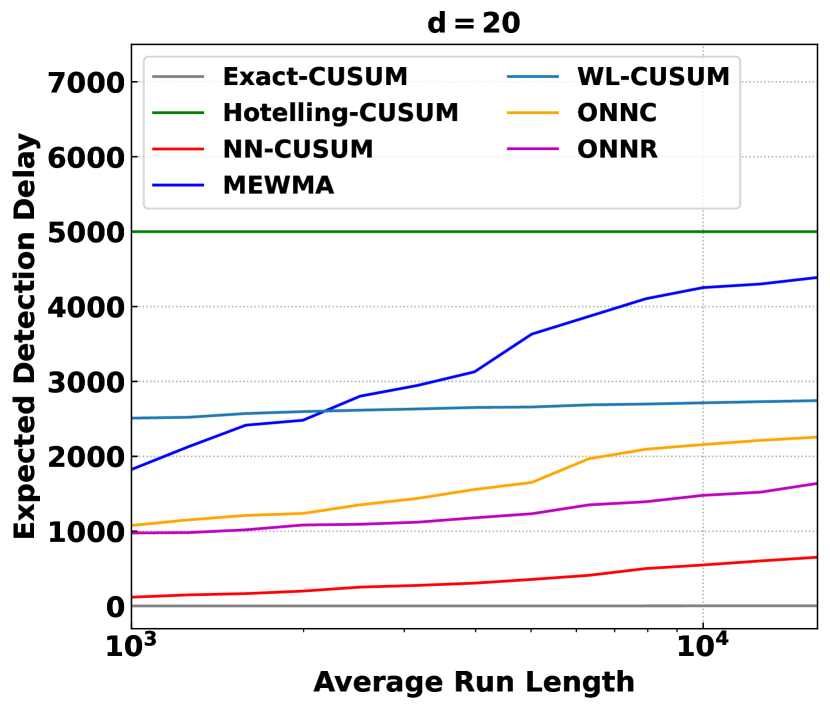
Figure A.7: EDD v.s. ARL Gaussian mixture model data with a component shift varing dimensions in $\{2,5,10,20\}$.

Appendix D Details of Datasets

D.1 Human Activity Change Detection

The dataset contains G-force measurements of several human activities from multiple individuals collected by portable 3D accelerometers. Therefore, each activity is a sequence of 3-dimensional data. Since the raw dataset includes noise, we chose one 20000-length sequence for each activity that shows the most stable pattern with minimum noises. Figure A.8 shows data sequences of the four activities up to 1000 time index.

D.2 Higgs Boson Detection

Higgs dataset contains two types of signal. The signal that produces Higgs bosons and background signal that does not produces Higgs bosons. Data of signal consist of 28 features where 21 features are kinematic properties measured by the particle detectors and 7 features are high-level features derived from the 21 kinematic features by physicists.

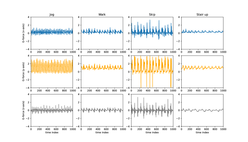
Figure A.8: Data sequences of the four activities (jog, walk, skip, and stair up) up to 1000 time index.

Appendix E Experimental Setup

E.1 Human Activity Change Detection

The stopping threshold for 0.05 type-I error was obtained by taking an average over 20 sequences of 1000-length pre-change activity. Each sequence consists of 500-length pilot sequence and 500-length online sequence. The expected detection delay was computed by averaging the detection delay of 10 of 1500-length sequences on the chosen threshold. Each 1500-length sequence consists of 500-length pilot sequence from pre-change activity and 1000-length online sequence from the post-change activity.

We use a fully connected neural network with one 512-width hidden layer. The training stack and testing stack size was set to 100 and 200, respectively. The batch size for training was set to 10 and the learning rate of the optimizer was set to 0.001. Stride was set to 2. Sensitivity analysis for the hyperparameters is available in Appendix F.

E.2 Higgs Boson Detection

The stopping threshold for 0.05 type-I error was obtained by taking an average over 20 sequences of 1000-length pre-change activity. Each sequence consists of 500-length pilot sequence and 500-length online sequence. The expected detection delay was computed by averaging the detection delay of 20 of 2000-length sequences on the chosen threshold. Each 2000-length sequence consists of 1000-length pilot sequence from pre-change activity and 1000-length online sequence from post-change activity.

The neural network architecture, setting of training and testing stack size, batch size, learning rate, stride are the same as in Human Activity data. The hyperparameter sensitivity analysis is given in Appendix F.

Appendix F Additional Real Data Experiments

We conducted additional experiments to explore the impact of hyperparameters on performance. For each experiment, all other hyperparameters except the tuning hyperparameter were set to the same setup as in Appendix E. We first investigated the effect of wider and deeper neural networks. Table A.1 and Table A.6 show EDD of NN-CUSUM with different network structures on human activity detection and Higgs boson detection, respectively. Table A.2 and Table A.3 show EDD of ONNC and ONNR with different network structures on human activity detection respectively. We also conducted experiments with $l_{2}$ loss in training. Table A.4 and Table A.7 show EDD of NN-CUSUM with $l_{2}$ training loss on human activity detection and Higgs boson detection, respectively. We finally conducted experiments with different strides. Table A.5 and Table A.8 show EDD of NN-CUSUM with different strides on human activity detection and Higgs boson detection, respectively.

We plotted EDD per method as violin plot to further investigate the results (Figure A.9 and Figure A.10). In human activity detection, we plotted EDD for each method without separating the results based on activity pair. We can observe that NN-CUSUM, ONNC, and ONNR show stable detection performance without any failure on human activity detection (Figure A.9). NN-CUSUM especially shows consistent performance with lower variances. On Higgs boson detection, NN-CUSUM, WL-CUSUM, and ONNC show stable detection performance without any failure in detection (Figure A.10). Specifically, NN-CUSUM achieved better detection performance than ONNC and WL-CUSUM on average.

Table A.1: Expected detection delay of NN-CUSUM with wider network structure and deeper network structure on human activity detection. The threshold was chosen by 0.05 type-I error. The standard deviation was reported in parentheses.

	layer=1, width=512	layer=1, width=1024	layer=2, width=512
Walk$\rightarrow$Stairup	$291.4{(36.5)}$	$249.6{(73.7)}$	$239.8{(115.0)}$
Jog$\rightarrow$Skip	$209.6{(30.6)}$	$159.4{(81.1)}$	$153.8{(117.5)}$
Skip$\rightarrow$Jog	$281.6{(50.0)}$	$364.4{(42.8)}$	$401.0{(50.3)}$
Stairup$\rightarrow$Walk	$371.4{(71.0)}$	$353.0{(79.4)}$	$339.8{(127.7)}$

Table A.2: Expected detection delay of ONNC with wider network structure and deeper network structure on human activity detection. The threshold was chosen by 0.05 type-I error. The standard deviation was reported in parentheses.

	layer=1, width=512	layer=1, width=1024	layer=2, width=512
Walk$\rightarrow$Stairup	$292.3{(146.8)}$	209.9 (120.5)	201.2 (140.4)
Jog$\rightarrow$Skip	$222.3{(83.8)}$	$305.1{(142.3)}$	$238.2{(102.7)}$
Skip$\rightarrow$Jog	$315.8{(95.5)}$	$533.7*{(265.8)}$	$534.3*{(289.8)}$
Stairup$\rightarrow$Walk	$477.7{(166.8)}$	$494.9{(187.8)}$	$477.4{(177.4)}$

Table A.3: Expected detection delay of ONNR with wider network structure and deeper network structure on human activity detection. The threshold was chosen by 0.05 type-I error. The standard deviation was reported in parentheses.

	layer=1, width=512	layer=1, width=1024	layer=2, width=512
Walk$\rightarrow$Stairup	$242.6{(136.5)}$	$236.6{(119.8)}$	$146.1{(95.2)}$
Jog$\rightarrow$Skip	$170.0{(77.1)}$	$66.9{(69.7)}$	$101.7{(77.7)}$
Skip$\rightarrow$Jog	$367.1{(81.9)}$	$68.5{(84.4)}$	$135.3{(107.9)}$
Stairup$\rightarrow$Walk	$347.0{(127.7)}$	$372.8{(145.6)}$	$305.2{(78.9)}$

Table A.4: Expected detection delay of NN-CUSUM with different training loss on human activity detection. The threshold was chosen by 0.05 type-I error. The standard deviation was reported in parentheses.

	logistic loss	$l_{2}$ loss
Walk$\rightarrow$Stairup	$291.4{(36.5)}$	$262.8{(85.1)}$
Jog$\rightarrow$Skip	$209.6{(30.6)}$	$159.2{(68.9)}$
Skip$\rightarrow$Jog	$281.6{(50.0)}$	$318.0{(38.8)}$
Stairup$\rightarrow$Walk	$371.4{(71.0)}$	$360.0{(77.8)}$

Table A.5: Expected detection delay of NN-CUSUM with different strides on human activity detection. The threshold was chosen by 0.05 type-I error. The standard deviation was reported in parentheses.

	stride=2	stride=4	stride=10
Walk$\rightarrow$Stairup	$291.4{(36.5)}$	$300.2{(69.0)}$	$323.0{(57.1)}$
Jog$\rightarrow$Skip	$209.6{(30.6)}$	$218.6{(74.8)}$	$284.0{(94.9)}$
Skip$\rightarrow$Jog	$281.6{(50.0)}$	$338.6{(57.9)}$	$314.0{(63.6)}$
Stairup$\rightarrow$Walk	$371.4{(71.0)}$	$349.0{(71.7)}$	$429.0{(83.8)}$

Table A.6: Expected detection delay of NN-CUSUM with wider network structure and deeper network structure on Higgs boson detection. The threshold was chosen by 0.05 type-I error. The standard deviation was reported in parentheses.

layer=1, width=512	layer=1, width=1024	layer=2, width=512
$425.5{(96.1)}$	$443.3{(137.1)}$	$440.6{(126.8)}$

Table A.7: Expected detection delay of NN-CUSUM with different training loss on Higgs boson detection. The threshold was chosen by 0.05 type-I error. The standard deviation was reported in parentheses.

logistic loss	$l_{2}$ loss
$425.5{(96.1)}$	$424.3{(161.9)}$

Table A.8: Expected detection delay of NN-CUSUM with different strides on Higgs boson detection. The threshold was chosen by 0.05 type-I error. The standard deviation was reported in parentheses.

stride=2	stride=4	stride=10
$425.5{(96.1)}$	$448.0{(123.9)}$	$431.5{(132.5)}$

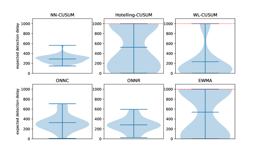
Figure A.9: Violin plot of EDD of NN-CUSUM and baselines on human activity change detection. Values on red dotted lines indicate failure in detection since maximum length of online sequence was 1000.

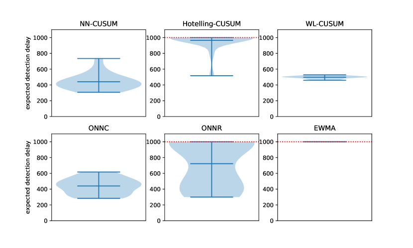
Figure A.10: Violin plot of EDD of NN-CUSUM and baselines on Higgs boson detection. Values on red dotted lines indicate failure in detection since maximum length of online sequence was 1000.

References

- [1] David Siegmund, Sequential analysis: tests and confidence intervals, Springer Science & Business Media, 1985.
- [2] Alexander Tartakovsky, Igor Nikiforov, and Michele Basseville, Sequential analysis: Hypothesis testing and changepoint detection, CRC Press, 2014.
- [3] H Vincent Poor and Olympia Hadjiliadis, Quickest detection, vol. 40, Cambridge University Press Cambridge, 2009.
- [4] Liyan Xie, Shaofeng Zou, Yao Xie, and Venugopal V Veeravalli, “Sequential (quickest) change detection: Classical results and new directions,” IEEE Journal on Selected Areas in Information Theory, vol. 2, no. 2, pp. 494–514, 2021.
- [5] Michael Baron, V Antonov, C Huber, M Nikulin, and VJL Polischook, “Early detection of epidemics as a sequential change-point problem,” Longevity, aging and degradation models in reliability, public health, medicine and biology, LAD, pp. 7–9, 2004.
- [6] Leto Peel and Aaron Clauset, “Detecting change points in the large-scale structure of evolving networks,” in Twenty-Ninth AAAI Conference on Artificial Intelligence, 2015.
- [7] Ming Qu, Frank Y Shih, Ju Jing, and Haimin Wang, “Automatic solar filament detection using image processing techniques,” Solar Physics, vol. 228, no. 1, pp. 119–135, 2005.
- [8] Zahra Ebrahimzadeh, Min Zheng, Selcuk Karakas, and Samantha Kleinberg, “Pyramid recurrent neural networks for multi-scale change-point detection,” 2018.
- [9] Zahra Atashgahi, Decebal Constantin Mocanu, Raymond Veldhuis, and Mykola Pechenizkiy, “Memory-free online change-point detection: A novel neural network approach,” arXiv preprint arXiv:2207.03932, 2022.
- [10] Muktesh Gupta, Rajesh Wadhvani, and Akhtar Rasool, “Real-time change-point detection: A deep neural network-based adaptive approach for detecting changes in multivariate time series data,” Expert Systems with Applications, vol. 209, pp. 118260, 2022.
- [11] George V Moustakides and Kalliopi Basioti, “Training neural networks for likelihood/density ratio estimation,” arXiv preprint arXiv:1911.00405, 2019.
- [12] Junghwan Lee, Yao Xie, and Xiuyuan Cheng, “Training neural networks for sequential change-point detection,” in ICASSP 2023-2023 IEEE International Conference on Acoustics, Speech and Signal Processing (ICASSP). IEEE, 2023, pp. 1–5.
- [13] Mikhail Hushchyn, Kenenbek Arzymatov, and Denis Derkach, “Online neural networks for change-point detection,” arXiv preprint arXiv:2010.01388, 2020.
- [14] Xiuyuan Cheng and Yao Xie, “Neural tangent kernel maximum mean discrepancy,” Advances in Neural Information Processing Systems, vol. 34, pp. 6658–6670, 2021.
- [15] Diederik P Kingma and Jimmy Ba, “Adam: A method for stochastic optimization,” arXiv preprint arXiv:1412.6980, 2014.
- [16] Arthur Gretton, Karsten M Borgwardt, Malte J Rasch, Bernhard Schölkopf, and Alexander Smola, “A kernel two-sample test,” The Journal of Machine Learning Research, vol. 13, no. 1, pp. 723–773, 2012.
- [17] Yao Xie and David Siegmund, “Sequential multi-sensor change-point detection1,” The Annals of Statistics, vol. 41, no. 2, pp. 670–692, 2013.
- [18] Gary Lorden, “Procedures for reacting to a change in distribution,” The annals of mathematical statistics, pp. 1897–1908, 1971.
- [19] David Siegmund and ES Venkatraman, “Using the generalized likelihood ratio statistic for sequential detection of a change-point,” The Annals of Statistics, pp. 255–271, 1995.
- [20] David Siegmund and Benjamin Yakir, “Detecting the emergence of a signal in a noisy image,” Statistics and its Interface, vol. 1, no. 1, pp. 3–12, 2008.
- [21] Pierre Baldi, Peter Sadowski, and Daniel Whiteson, “Searching for exotic particles in high-energy physics with deep learning,” Nature communications, vol. 5, no. 1, pp. 4308, 2014.
- [22] Nobuo Kawaguchi, Nobuhiro Ogawa, Yohei Iwasaki, Katsuhiko Kaji, Tsutomu Terada, Kazuya Murao, Sozo Inoue, Yoshihiro Kawahara, Yasuyuki Sumi, and Nobuhiko Nishio, “Hasc challenge: gathering large scale human activity corpus for the real-world activity understandings,” in Proceedings of the 2nd augmented human international conference, 2011, pp. 1–5.
- [23] “Higgs data set,” https://archive.ics.uci.edu/ml/datasets/HIGGS.
- [24] Liyan Xie, George V Moustakides, and Yao Xie, “Window-limited cusum for sequential change detection,” arXiv preprint arXiv:2206.06777, 2022.
- [25] Cynthia A Lowry, William H Woodall, Charles W Champ, and Steven E Rigdon, “A multivariate exponentially weighted moving average control chart,” Technometrics, vol. 34, no. 1, pp. 46–53, 1992.