Anomaly Detection in Additive Manufacturing Processes using Supervised Classification with Imbalanced Sensor Data based on Generative Adversarial Network

Abstract

Supervised classification methods have been widely utilized for the quality assurance of the advanced manufacturing process, such as additive manufacturing (AM) for anomaly (defects) detection. However, since abnormal states (with defects) occur much less frequently than normal ones (without defects) in a manufacturing process, the number of sensor data samples collected from a normal state is usually much more than that from an abnormal state. This issue causes imbalanced training data for classification analysis, thus deteriorating the performance of detecting abnormal states in the process. It is beneficial to generate effective artificial sample data for the abnormal states to make a more balanced training set. To achieve this goal, this paper proposes a novel data augmentation method based on a generative adversarial network (GAN) using additive manufacturing process image sensor data. The novelty of our approach is that a standard GAN and classifier are jointly optimized with techniques to stabilize the learning process of standard GAN. The diverse and high-quality generated samples provide balanced training data to the classifier. The iterative optimization between GAN and classifier provides the high-performance classifier. The effectiveness of the proposed method is validated by both open-source data and real-world case studies in polymer and metal AM processes.

1 Introduction

Advanced manufacturing processes, such as additive manufacturing (AM), are widely applied in various fields, including aerospace, healthcare, and the automotive industry (Liu et al., 2019). However, a major barrier preventing broader industrial adoption of the processes is the quality assurance of products. For example, surface defects exist, such as under-fill from the Fused Filament Fabrication (FFF) process shown in Fig. 1. It is due to highly complex interactions in consecutive layers during printing. The defect causes a deficiency in the mechanical properties of the final product, such as density, tensile strength, and compressive strength (Hajalfadul and Baumers, 2021). Therefore, timely detection of the anomaly in the process is necessary so that corrective actions can be taken to mitigate the defects and improve the quality of products (Makes and Collaborative, 2017).

Recently, the development of sensor technologies and computational power offered online process data, providing excellent opportunities to achieve effective quality assurance through a data-driven approach (Liu et al., 2021). Specifically, the sensor data are usually in high volume in terms of both dimensionality and sampling frequency, having plenty of information about the manufacturing processes (Zhou et al., 2020). Therefore, it is very beneficial to investigate the underlying relationships between the sensor data and process quality state based on a data-driven perspective (Li et al., 2021). Utilizing the sensor data, supervised classification methods have been widely applied to online anomaly detection in the manufacturing process (Banadaki et al., 2020; Jin et al., 2019; Guo et al., 2019). This is because these methods can fully utilize the label information of the process state, resulting in more accurate and reliable detection results than unsupervised methods. Banadaki et al. (2020); Jin et al. (2019); Guo et al. (2019) utilized balanced training data collected from both normal and abnormal states in the manufacturing processes to achieve a high anomaly detection rate from classifiers (Choi et al., 2021).

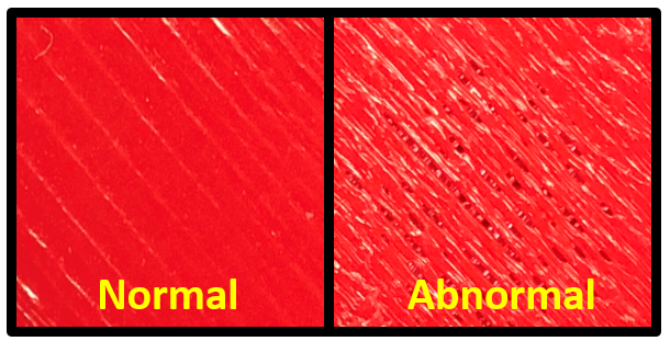
Figure 1: Normal surface and Abnormal defect in AM process.

However, the manufacturing process is usually in a normal state (Li et al., 2021). Therefore, balanced training data assumed by the existing work (Banadaki et al., 2020; Jin et al., 2019) is expensive and not realistic. In reality, abnormal conditions, such as surface defects in AM process (Fig. 1), may happen but rarely. Consequently, the sensor data collected under abnormal states are smaller than those collected in a normal state, and may not be sufficient for training supervised classification methods. It causes imbalanced training data among process states (Chawla et al., 2004), leading to compromised anomaly detection performance in actual manufacturing processes (Li et al., 2021). Specifically, when the number of training data samples from a normal state is significantly more than that of abnormal states, the prediction in classification models tends to be biased towards the normal state (i.e., majority class) (Choi et al., 2021). This leads to a high probability of misclassifying samples from the abnormal states (i.e., minority classes).

To overcome this severe issue caused by imbalanced data problems in the manufacturing process, data augmentation can be applied to obtain balanced training data among process states. Simple data augmentation techniques such as rotation, flipping, and synthetic minority oversampling technique (SMOTE) (Chawla et al., 2002) are widely used for balancing training data in the supervised classification method for the manufacturing process because of their simplicity in application (Cui et al., 2020; Lee et al., 2020; Mycroft et al., 2020). However, such methods consider only local information; therefore, they cannot reflect the entire data distribution and overcome the problem of overfitting (Douzas and Bacao, 2018; Mikołajczyk and Grochowski, 2018). As a result, these methods are unsuitable for generating realistic and diverse data on abnormal states in manufacturing applications (Fathy et al., 2020; Ranasinghe and Parlikad, 2019). Recently, the generative adversarial network (GAN) (Goodfellow et al., 2014) has been actively used for data augmentation in manufacturing. This is because GAN generates more representative data than the simple augmentation method by learning the entire distribution of actual data through two neural networks: discriminator and generator (Antoniou et al., 2017; Kiyasseh et al., 2020). For example, Gobert et al. (2019) used conditional GAN to generate layer images from the metal AM process. In addition, Li et al. (2021) developed a novel GAN method considering temporal orders of the sensor signal from the polymer AM process to generate the balanced training signal data.

Utilizing GAN, the existing studies achieved high classification performance by training the classifier with the generated balanced training samples. The generated samples of each process state are realistic by learning the distribution of actual data. However, features enabling differentiation between process states (i.e., state-distinguishable features) that can further improve the classification performance have not been considered in the generation process from GAN in the previous studies (Gobert et al., 2019; Li et al., 2021).

This paper proposes a novel GAN-based data augmentation method in manufacturing to generate realistic and state-distinguishable generated data. Compared to a standard GAN consisting of two players, i.e., discriminator and generator, the proposed method comprises three players, including a classifier. All players are jointly optimized in the proposed approach to meet their respective goals. Specifically, the generator learns to generate data deceiving the discriminator. In contrast, a discriminator learns to distinguish whether data is from a generator or an actual process. This adversarial learning results in generating realistic samples from the generator. At the same time, the generator and classifier cooperate to generate distinctive samples among process states in the manufacturing process. Specifically, the classifier guides the generator to create samples that could benefit classification results. Then, the classifier is trained with balanced training data supplemented from generated samples of abnormal states. This iterative learning among three-player finally provides the classifier with high performance.

Furthermore, the proposed method provides two terms in the objective function of the discriminator to improve the training stability of standard GAN. First, the proposed method regularizes the gradient of the discriminator (Fedus et al., 2017). Second, the proposed approach provides an additional task to the discriminator compared to standard GAN, preventing the discriminator from discerning the origin of data very well (Huang and Jafari, 2021). Both terms improve the training stability by preventing gradient exploding in training the generator. The contributions of this work are summarized as follows:

• From the methodological point of view, this paper proposes a novel data augmentation method that standard GAN and classifier are jointly optimized with techniques to stabilize the learning process of standard GAN. The generated samples from the generator provide balanced training data to the classifier. The iterative optimization between GAN and classifier provides a classifier with superior performance.

• From the application perspective, the proposed method is applied to anomaly detection in actual additive manufacturing processes. The technique successfully detects process anomalies when highly imbalanced data sets exist. The effectiveness of the proposed method is validated from polymer and metal AM processes, namely, Fused Filament Fabrication (FFF) and Electron Beam Melting (EBM) processes.

The rest of this paper is organized as follows. A brief review of related research work is provided in Section 2. The proposed methodology is presented in Section 3, followed by case studies with open-source and actual AM data sets to validate its effectiveness in Section 4. Finally, conclusions are discussed in Section 5.

2 Review of Related Work

The relevant existing studies on anomaly detection approaches for the manufacturing processes are briefly reviewed first in Section 2.1, and subsequently, the existing data augmentation methods are summarized in Section 2.2. Afterward, the research gaps in the current work are identified in Section 2.3.

2.1 Anomaly Detection Approaches for the Manufacturing Processes

The anomaly detection approaches for manufacturing processes have been extensively studied. Recently, deep learning-based methods have been widely used. For example, Kyeong and Kim (2018) proposed using convolutional neural networks (CNNs) to classify mixed-type defect patterns in wafer bin maps in the semiconductor manufacturing process. Kwon et al. (2020) used deep neural networks to accurately classify melt pool images in the metal AM process concerning different laser powers, resulting in different porosity levels. Zhang et al. (2020) converted the vibration signal from the drive end bearing to the images. The images were used as training data for CNN for bearing fault diagnosis. In addition, Jia et al. (2019) applied CNN to extract the features from the infrared thermal images for the fault diagnosis of rotating machinery in the manufacturing process.

In addition to the deep learning-based methods, various machine learning-based methods are utilized in anomaly detection in the manufacturing processes. For example, Montazeri and Rao (2018) proposed a graph-theoretic approach to differentiate the distinctive thermal signatures of melt pool images, leading to poor abnormal surface finish from the metal AM process. Mahmoudi et al. (2019) also developed a novel anomaly detection framework in the metal AM process. The approach classified the process state by accounting for the spatial dependence among successive melt pools through the Gaussian process. For the polymer AM process, Liu et al. (2021) proposed a feature extraction method based on manifold learning to diagnose surface defects such as under-fill. Shen et al. (2020) also proposed a novel supervised feature extraction method to extract discriminant and informative features from the surface states in the FFF process. In addition to the several AM processes, Bhat et al. (2016) presented a classification method to diagnose the cutting tool condition in the manufacturing process by analyzing the machined surface. Specifically, a kernel-based support vector machine classifier was trained with the features extracted from the gray-level co-occurrence matrix of machined surface images. Wang and Chen (2019) proposed weight masks to extract rotation-invariant features for wafer map failure pattern detection in the semiconductor manufacturing process.

2.2 Data Augmentation Methods

The existing data augmentation methods from the literature can be divided into two categories, sampling-based approaches, e.g., an oversampling technique, and deep learning-based approaches, e.g., GAN.

Sampling-based approaches such as oversampling methods generate synthetic samples based on the existing samples, including interpolation, to balance the data. The most popular oversampling method is the synthetic minority oversampling technique (SMOTE) proposed by Chawla et al. (2002). It also has several extensions (Fernández et al., 2018). For example, many rules for regions of data to be oversampled are settled down, such as Borderline-SMOTE (B-SMOTE) (Han et al., 2005) and the adaptive synthetic sampling approach (ADASYN) (He et al., 2008). Furthermore, there exist hybrid methods, such as SMOTE editing the nearest neighbor (SMOTENN) (Batista et al., 2004) and SMOTE-Iterative partitioning filter (SMOTE-IPF) (Sáez et al., 2015). They remove unsuitable samples after SMOTE-based oversampling.

Recently, deep learning has become popular in data augmentation due to its powerful computation for high-dimensional data (Shorten and Khoshgoftaar, 2019). GAN is one of the most widely applied approaches, which was first introduced by Goodfellow et al. (2014). GAN-based work for data augmentation exploits the GAN models, such as deep convolutional GAN (DCGAN) (Wang et al., 2017), cycle GAN (Zhang, 2018), and conditional GAN (cGAN) (Douzas and Bacao, 2018) to supplement the limited actual data by generated data. Balancing GAN (BAGAN) (Mariani et al., 2018) is a modified version of an auxiliary classifier GAN (Odena et al., 2017) that focuses on the generation of minority class samples. Moreover, Huang and Jafari (2021) proposed an enhanced version of BAGAN (BAGAN-GP) that overcomes the unstable training issue in BAGAN by providing an improved initialization method and gradient penalty technique (Gulrajani et al., 2017). Recently, Choi et al. (2021) proposed a three-player GAN that consists of a discriminator, generator, and classifier. In this method, the processes of generating samples and training classifiers are jointly optimized. It generates both realistic and state-distinguishable generated samples that are beneficial to improving the classification results. However, this work follows a standard GAN structure (Goodfellow et al., 2014) that is prone to unstable learning resulting in limited diversity and poor quality of generated samples (Zhu et al., 2019).

2.3 Research Gap Analysis

The studies summarized in Section 2.1 contributed to anomaly detection in the manufacturing process. However, the work does not consider the imbalanced training data that usually occurs in reality. Instead, the literature requires sufficient data from abnormal states, which is highly time-consuming and prohibitively costly. Research efforts in Section 2.2 provided data augmentation work to overcome the imbalanced training data issue in the manufacturing process. However, the sampling-based methods consider only local information; therefore, they cannot reflect the entire data distribution (Douzas and Bacao, 2018). Recently, GAN-based methods have been widely used because of their superior performance in data augmentation. However, the process of generating samples through GAN and the process of training a classifier with the generated samples are handled independently in most of the studies. It is critical to generate realistic samples that follow the distribution of actual samples through GAN. However, it is also important that the generated samples help improve the classifier performance as training data. To achieve this, the realistic samples must be well-distinguishable among the process states. Thus, this paper proposes a novel GAN-based data augmentation method for additive manufacturing applications where the processes of generating samples and training a classifier are jointly optimized. Furthermore, the proposed method regularizes the gradient of the discriminator and provides an additional task to the discriminator compared to standard GAN. This improves the training stability that prevents gradient exploding of the generator. It results in a better quality of generated samples, improving the classifier’s performance compared to the existing work. The effectiveness of the proposed method is validated with imbalanced surface images from actual AM processes described in Section 4.

3 Proposed Research Framework

This section proposes a novel GAN-based data augmentation method. The structure of the proposed method is illustrated in Section 3.1. Specifically, the objective function of the proposed method is described in Section 3.2, followed by the training procedure in Section 3.3.

3.1 Three-Player Structure for Imbalanced Data Learning

Fig. 2 shows the structure of the proposed method, which consists of three players: a discriminator, a generator, and a classifier.

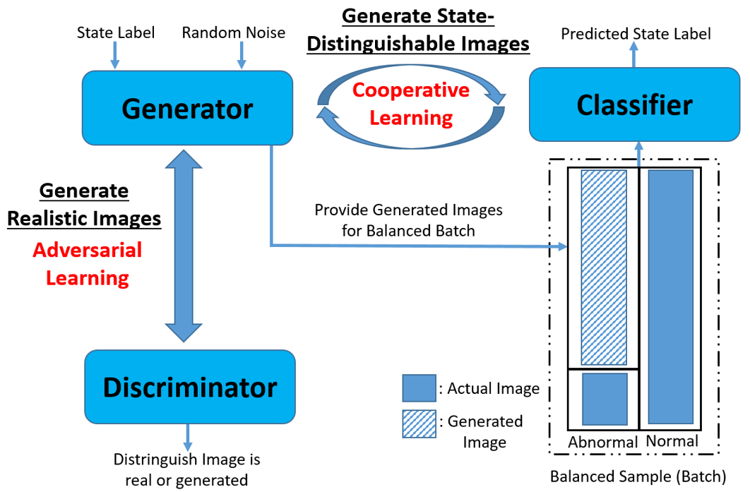
Figure 2: Structure of the proposed method.

The generator generates images of the manufacturing process from the random noise and corresponding state label. Among the generated images, the images of abnormal states are combined with the actual imbalanced manufacturing process images, providing a balanced training sample to the classifier. The proposed method offers adversarial and cooperative learning to make the generated images beneficial to the classifier’s performance. The roles of these two are provided as follows.

• Adversarial learning: The relationship between discriminator and generator follows the adversarial relationship from the GAN structure. The relationship enables both networks to compete with each other, resulting in realistic generated samples of the manufacturing process from the generator.

• Cooperative learning: The cooperative relationship between the generator, and the classifier enables the generator to generate samples that are distinguishable among process states in the manufacturing process (i.e., state-distinguishable samples) from the classifier.

Based on these two relationships, the generator generates samples of abnormal states in the manufacturing process with both properties (i.e., realistic and state-distinguishable). The generated samples are added to actual ones and provided as a balanced training batch that the number of training samples passing through the network at one time of a classifier. The iterative learning process among these three players finally provides a classifier with high performance. The detailed objective function and training procedures are explained in the following sections.

3.2 Objective Functions for Three-Player

In this subsection, the review of the generative adversarial network in the manufacturing process is described in Section 3.2.1 initially. Then, the objective functions of the discriminator, generator, and classifier are illustrated in Sections 3.2.2, 3.2.3, and 3.2.4, respectively.

3.2.1 Generative Adversarial Network in the Manufacturing Process

The idea of a Generative Adversarial Network (GAN) is to train two networks, namely, generator $G$ and discriminator $D$, with a minimax game for $V(D,G)$ demonstrated in Eq. (1) (Wang et al., 2017).

$$\min_{G}\max_{D} V(D,G)=\mathbb{E}_{x_{a}\sim P(X_{a})}[\text{log}(D(x_{a}))]$$ (1)

$$+\mathbb{E}_{z\sim P({Z})}[\text{log}(1-D(G(z))],$$

where $z$ is the random noise, and $x_{a}$ denotes actual samples from the manufacturing process. Specifically, the generator is to generate samples of the manufacturing process $G(z)$ from $z$, and the discriminator is to distinguish whether the origin of input samples is from actual ($x_{a}$) or generator ($G(z)$). In other words, the discriminator is to discern the input samples, while the generator synthesizes artificial samples to deceive the discriminator. This adversarial learning results in the distribution of newly generated samples, close to the underlying distribution of the actual samples in the manufacturing process, $P(X_{a})$.

As shown in Fig. 2, the proposed method needs to provide balanced training samples among the manufacturing process states in every batch of a classifier. To achieve this, conditional GAN (Douzas and Bacao, 2018) is applied in the proposed method making the process state label attached to the input of the generator and discriminator. It enables users to determine the number of generated samples from abnormal states of the manufacturing process to make a balanced batch. The objective function of conditional GAN is demonstrated in Eq. (2) as follows.

$$\min_{G}\max_{D} V(D,G)=\mathbb{E}_{(x_{a},y_{a})\sim P(X_{a},Y_{a})}[\text{log}(D(x_{a},y_{a}))]$$ (2)

$$+\mathbb{E}_{(z,y_{g})\sim P(Z,Y_{g})}[\text{log}(1-D(G(z,y_{g}),y_{g})],$$

where $y_{a}$ and $y_{g}$ denote the process state label of an actual and generated sample, respectively.

3.2.2 Objective Function of Discriminator

The objective of the discriminator in the proposed method is to maximize Eq. (2) through adversarial learning with the generator. Specifically, the discriminator learns to distinguish the input ($x_{a},y_{a}$) and ($G(z,y_{g}),y_{g}$) are actual and generated, respectively. In addition, the proposed method provides two additional terms for stabilizing the learning process, as the training of the GAN is unstable and challenging to converge due to the gradient exploding issue in adversarial learning (Tao and Wang, 2020; Arjovsky and Bottou, 2017).

First, the proposed method regularizes the gradient of the discriminator by providing the gradient penalty in the form of Eq. (3) as follows.

$$\mathbb{E}_{(\hat{x},y_{a})\sim P(\hat{X},Y_{a})}[(\lVert\nabla_{(\hat{x},y_{a})}D(\hat{x},y_{a})\rVert_{2}-1)^{2}],$$ (3)

where $\hat{x}=\alpha x_{a}+(1-\alpha)G(z)$, and $\alpha$ is sampled uniformly between 0 and 1. It enforces 1-Lipschitz continuity to the discriminator (Davenport, 1951). The term is widely used in the previous work (Gulrajani et al., 2017; Fedus et al., 2017; Huang and Jafari, 2021) to overcome the limited diversity and poor quality of generated samples from GAN caused by unstable adversarial learning.

Second, the proposed method provides an additional input consisting of the actual sample ($x_{a}$) and a mislabeled process state ($y_{m}$) to the discriminator. The discriminator learns to distinguish that the input ($x_{a},y_{m}$) is not an actual but generated sample because of the mislabeled process state by minimizing the following quantity.

$$-\mathbb{E}_{(x_{a},y_{m})\sim P(X_{a},Y_{m})}[\text{log}(1-D(x_{a},y_{m})],$$

where $y_{m}$ is randomly sampled from the remaining labels in the manufacturing process except for the actual state label. Since the input provides an additional task for the discriminator to learn, it prevents the discriminator distinguishes very well between actual and generated samples before the generator approximates the actual sample distribution of the manufacturing process. Otherwise, it causes unstable learning of GAN through exploding or vanishing the gradient of the generator (Tran et al., 2018; Arjovsky and Bottou, 2017).

In summary, the objective function of the discriminator ($L^{D}$) in the proposed method is to minimize the following equation consisting of several losses.

$$L^{D}( Z,X_{a},Y_{a},Y_{g},Y_{m})=$$ (4)

$$\underbrace{-\mathbb{E}_{(x_{a},y_{a})\sim P(X_{a},Y_{a})}[\text{log}(D(x_{a},y_{a}))]}_{\text{loss from actual sample in discriminator}}$$

$$\underbrace{-\mathbb{E}_{(z,y_{g})\sim P(Z,Y_{g})}[\text{log}(1-D(G(z,y_{g}),y_{g})]}_{\text{loss from generated sample in discriminator}}$$

$$\underbrace{-\mathbb{E}_{(x_{a},y_{m})\sim P(X_{a},Y_{m})}[\text{log}(1-D(x_{a},y_{m})]}_{\text{loss from mislabeled sample in discriminator}}$$

$$+\lambda\underbrace{\mathbb{E}_{(\hat{x},y_{a})\sim P(\hat{X},Y_{a})}[(\lVert\nabla_{(\hat{x},y_{a})}D(\hat{x},y_{a})\rVert_{2}-1)^{2}]}_{\text{loss from gradient penalty}},$$

where $\lambda$ is the coefficient of the gradient penalty term. The first three losses in Eq. (4) are related to losses when the discriminator misclassified the origin of the actual, generated, and mislabeled sample. The last loss represents the loss related to the gradient of the discriminator.

3.2.3 Objective Function of Generator

The objective of the generator is to generate samples via learning the distribution of actual samples of the manufacturing process ($P(X_{a})$) by minimizing Eq. (2). Alternatively, the proposed method trains the generator to maximize Eq. (5) to avoid the saturation problem occurring when minimizing Eq. (2) in practice (Goodfellow et al., 2014).

$$\mathbb{E}_{(z,y_{g})\sim P(Z,Y_{g})}[\text{log}(D(G(z,y_{g}),y_{g})].$$ (5)

In addition to Eq. (5), the generator in the proposed method has an additional term in the objective function related to the classifier. In contrast to an adversarial relationship with a discriminator, the cooperative relationship is designed between the generator and classifier to generate well-distinguishable samples among process states in the manufacturing process. To achieve this, the classification loss from labels of generated samples is provided to the objective function of the generator (2 term in Eq. (6)). Finally, the generator in the proposed method is trained by minimizing its objective function ($L^{G}$), Eq. (6).

$$L^{G}(Z,Y_{g})= \underbrace{-\mathbb{E}_{(z,y_{g})\sim P(Z,Y_{g})}[\text{log}(D(G(z,y_{g}),y_{g}))]}_{\text{loss from generated sample in discriminator}}$$ (6)

$$\underbrace{-\mathbb{E}_{(z,y_{g})\sim P(Z,Y_{g})}[y_{g}\text{log}(C(G(z,y_{g})))]}_{\text{loss from generated sample in classifier}},$$

where $-\mathbb{E}_{(z,y_{g})\sim P(Z,Y_{g})}[y_{g}\text{log}(C(G(z,y_{g})))]$ (2 term in Eq. (6)) denotes the cross-entropy loss of generated samples from the classifier.

3.2.4 Objective Function of Classifier

The objective function of the classifier ($L^{C}$) consists of the classification loss from both actual and generated samples of the manufacturing process as Eq. (7). As described in Fig. 2, the samples from the generator are supplemented with actual samples from the manufacturing process to make balanced training data in every batch of the classifier. The classifier is optimized to minimize the classification loss from both actual and generated sample by minimizing Eq. (7).

$$L^{C}(Z,X_{a}, Y_{a},Y_{g})=\underbrace{-\mathbb{E}_{(x_{a},y_{a})\sim P(X_{a},Y_{a})}[y_{a}\text{log}(C(x_{a}))]}_{\text{loss from actual sample in classifier}}$$ (7)

$$\underbrace{-\mathbb{E}_{(z,y_{g})\sim P(Z,Y_{g})}[y_{g}\text{log}(C(G(z,y_{g}))]}_{\text{loss from generated sample in classifier}}.$$

In particular, $-\mathbb{E}_{(z,y_{g})\sim P(Z,Y_{g})}[y_{g}\text{log}(C(G(z,y_{g}))]$, a common term in both Eqs. (6) and (7) enables cooperative learning between the generator and classifier.

3.3 Training Procedure

To train the three players in the proposed method, the method adopts an alternating gradient descent method among the training of generator, discriminator, and classifier. Before starting alternating optimization, the auto-encoder is pre-trained with the existing imbalanced samples from the manufacturing process. Auto-encoder is trained to minimize the reconstruction error of inputs. Auto-encoder is widely used for the initialization of the generator in GAN because it leads to stable learning and helps the generator learn common data set knowledge (Mariani et al., 2018). The pre-trained decoder from an auto-encoder is initialized as the generator in the proposed method. After the pre-training step, the three players are optimized alternatively. First, the discriminator is trained with a batch from actual and generated samples to minimize Eq. (4). Sequentially, a batch from generated samples is utilized to update the generator by minimizing Eq (6). Finally, the classifier is trained by minimizing Eq. (7) with balanced training data from all the process states in the manufacturing process. Specifically, a batch ($m$) from actual data is sampled first. Then, the remaining samples from abnormal states ($m_{g}$) are generated from the generator to make a balanced training set. The alternating training procedure is iterated until it reaches the pre-defined epochs. The overall training procedure of the proposed method is illustrated in Algorithm 1. The parameters of a discriminator, generator, and classifier are denoted as $\theta_{d},\theta_{g},$ and $\theta_{c}$, respectively.

Initialize the parameters of three players (i.e., $\theta_{d}$, $\theta_{g}$, and $\theta_{c}$).

            P-Epoch: Number of epochs in the pre-training.

            A-Epoch: Number of epochs in the alternating loop.

            Batch size: Size of samples ($m$) in each batch.

Procedure:

           [Pre-Training Generator]

                 Initialize: epoch=1

                 while epoch $\leq$ P-Epoch do

                   Sample a batch of $m$ samples from $X_{a}$

                   Train auto-encoder ($\theta_{g}$)

                   epoch + +

                 end while

            [Alternating Optimization]

                 Initialize: epoch=1

                 while epoch $\leq$ A-Epoch do

                    Sample $m$ samples from $X_{a},Z,Y_{g},Y_{m}$

                    Train a discriminator $(\theta_{d})$ by minimizing Eq. (4)

                    Sample $m$ samples from $Z,Y_{g}$

                    Train a generator $(\theta_{g})$ by minimizing Eq. (6)

                    Sample $m$ samples from $X_{a}$

                    Sample $m_{g}$ from $Z,Y_{g}$ of abnormal states to balance the batch                     Train a classifier $(\theta_{c})$ by minimizing Eq. (7)

                    epoch + +

                  end while

Algorithm 1 Training Procedures of the proposed method.

4 Real-World Case Studies

Several real-world case studies are provided to show the effectiveness of the proposed method. Section 4.1 demonstrates the advantages of the proposed method based on the ablation study. The method is deeply self-analyzed in various aspects. Sections 4.2, 4.3, and 4.4 provide comparative case studies with benchmark methods across multiple data sets. Specifically, open-source data set is used in Section 4.2. In addition, the surface image data from two actual AM processes, namely, Fused Filament Fabrication (FFF) and Electron Beam Melting (EBM) processes, are utilized in Sections 4.3 and 4.4, respectively, to demonstrate the effectiveness of the proposed method in an actual AM process. The performance is evaluated by the classification results from the imbalanced training data set. The framework of all case studies is Keras with TensorFlow backend. The studies are performed by an NVIDIA Tesla P4 GPU with 8GB memory.

1) Benchmark Methods: For the benchmark methods, both the sampling-based and GAN-based approaches described in Section 2.2 are used. In the sampling-based methods, SMOTE (Chawla et al., 2002), B-SMOTE (Han et al., 2005), and ADASYN (He et al., 2008), which are implemented in the imbalanced-learn library in python, are adopted. For the GAN-based approaches, two state-of-the-art methods, CDRAGAN (Huang and Jafari, 2021), and BAGAN-GP (Huang and Jafari, 2021) are selected. In addition, Cooperative GAN (Choi et al., 2021), which jointly optimizes GAN and the classifier, is determined as one of the benchmark methods. Finally, classification performance without any data augmentation method is provided as the baseline.

2) Hyperparameters and Experimental Settings: The optimizer for the proposed method is the Adam algorithm (Kingma and Ba, 2014) with a learning rate of 0.0002 and momentums of 0.5 and 0.9 (Huang and Jafari, 2021). To make the networks in the proposed method irrespective of the image size, all the image inputs are resized as 64$\times$64$\times$channels. The dimension of the random noise ($z$) is 128. Since the proposed method deals with image data, the auto-encoder with convolution layers is used for pre-training (Huang and Jafari, 2021). In addition, the discriminator and generator are designed with a convolution layer, leakyReLu layer, and transpose convolution layer. For the classifier, Convolutional Neural Network (CNN) is utilized in the case studies since CNN extracts the features from the raw data directly, resulting in superior performance in image classification (Dhillon and Verma, 2020). For a fair comparison, the CNN with the same hyperparameters is used for all the methods. Besides, the unique hyperparameters of each method, such as the scheduling parameter in the Cooperative GAN (Choi et al., 2021), are searched within a specific range following the guidelines provided in the literature and determined with the values that showed the best performance. The detailed hyperparameters of the generator, discriminator, and classifier are provided in Appendix A.

3) Performance Evaluation Measure: The classification performance is evaluated by the value of the F-score, Precision, and Recall (Powers, 2020). Precision and Recall are related to the level of type I and type II errors, respectively. F-score can be formulated by Eq. (8), which is the combination of Precision and Recall.

$$\text{F-score}=2\times\frac{\text{Precision}\times\text{Recall}}{\text{Precision}+\text{Recall}}.$$ (8)

Since this paper aims to improve the classification accuracy with the imbalanced training data, case studies with various balanced ratios are provided. A balanced ratio is the ratio between the training data size of the minority and the majority classes. All the case studies were repeated ten times, and the average of ten repetitions was provided as the performance measure.

4.1 Ablation Studies

The ablation study is conducted with MNIST fashion data (Xiao et al., 2017). From the 1000 images of each of three labels, namely, T-shirt, Pullover, and Dress, imbalanced training data is constructed as described in Table 1. To provide the challenging task, the balanced ratio between the majority and minority classes is 0.10. The remaining images are used as testing data.

Table 1: Imbalanced training data samples in ablation studies.

Data Set	Majority Class	Minority Class	Balanced Ratio	Majority Class Training Samples	Minority Class Training Samples
MNIST fashion	T-shirt	Pullover, Dress	0.10	800	80

The study is carried out by sequentially adding each ablation component since each component cannot be implemented without the previous components. The role of each component is validated through the ablation of a baseline and three variants, as illustrated in Table 2. Baseline trains classifier with imbalanced training data without any data augmentation. Instead, Variant 1 uses a conditional version of standard GAN (i.e., CGAN (Mirza and Osindero, 2014)) to provide balanced training data of the classifier by generating additional minority class samples ($G(z,y_{g})$ in Section 3). Furthermore, Variant 2 jointly trains the classifier and CGAN by providing cross-entropy losses ($y_{g}\text{log}(C(G(z,y_{g})))$, and $y_{a}\text{log}(C(x_{a}))$ in Section 3) so that the generator in the CGAN produces distinctive samples among the process states. Finally, Variant 3, which is the proposed method, adds the terms ($\lVert\nabla D(\hat{x},y_{a})\rVert_{2}$, and $D(x_{a},y_{m})$ in Section 3) that are related to stabilizing the learning process in the objective function of the discriminator in Variant 2.

Table 2 shows the results of the ablation study. In addition to F-score, Precision, and Recall, Frechet Inception Distance (Dowson and Landau, 1982) (FID) is used as an additional performance measure in the ablation study. FID is a metric used to evaluate the quality of images generated by GAN. Specifically, it is a metric between two multidimensional Gaussian distributions that are the distribution of neural network features from the actual and generated images, respectively. FID is computed from the mean and the covariance of the activation function of the network as follows:

$$\text{FID}=\lVert\mu_{a}-\mu_{g}\rVert^{2}+\text{Tr}(\Sigma_{a}+\Sigma_{g}-2(\Sigma_{a}\Sigma_{g})^{1/2}),$$

where $\mu_{a}$ and $\Sigma_{a}$ are the mean and standard deviation from actual images, respectively; likewise, $\mu_{g}$ and $\Sigma_{g}$ are those from generated images, respectively. The smaller FID represents that the generated images follow the distribution of actual images resulting in better quality and diversity (Chen et al., 2021). In Table 2, the FID scores of each label are presented. 1500 images of each label from actual and generated images, respectively, are used to calculate the FID.

Table 2: Performance evaluation in ablation studies.

	$G(z,y_{g})$	$y_{a}\text{log}(C(x_{a})),$ $y_{g}\text{log}(C(G(z,y_{g})))$	$\lVert\nabla D(\hat{x},y_{a})\rVert_{2},$ $D(x_{a},y_{m})$	F-score	Precision	Recall	FID T-shirt	FID Pullover	FID Dress
Baseline	✗	✗	✗	0.783	0.785	0.873	NA	NA	NA
Variant1	✓	✗	✗	0.791	0.789	0.879	203.9	239.9	226.1
Variant2	✓	✓	✗	0.806	0.797	0.886	192.3	234.9	227.9
Variant3 (Proposed)	✓	✓	✓	0.830	0.814	0.900	109.3	142.9	184.3

The performance of all the measures of Variant 1 improves compared to the baseline. It shows the effectiveness of GAN for supplementing imbalanced training data. In Variant 2, an improvement in the performance of most of the measures is achieved compared to the first ablation. This implies that joint training of GAN and classifier guides the generator to generate samples beneficial to the classifier, that is, both realistic and state-distinguishable samples. It consequently improves the performance of the classifier. Finally, when both terms stabilizing the learning process of GAN are added, which is the proposed method (Variant 3), the performances are significantly improved since stable training enables the generator to generate more realistic and state-distinctive samples. Specifically, Fig. 3 compares the log scale norm for the gradient of the generator ($\log(\nabla\lVert L^{G}(Z,Y_{g})\rVert$) between Variant 2 and the proposed method. The results show the gradient of the proposed method decreases with the small variance, while the gradient of Variant 2 explodes with a large variance, resulting in unstable learning and low-quality generated samples (Arjovsky and Bottou, 2017).

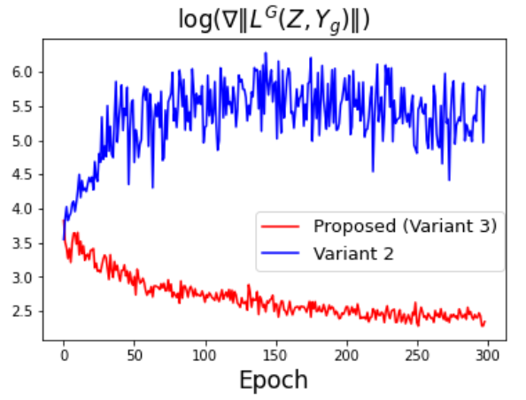
Figure 3: Comparison of a log scale norm for the gradient of the generator.

Fig. 4 shows the quality of generated images in each step of the ablation study. Fig. 4 (a) represents the actual images from each label. Figs. 4 (b), (c), and (d) illustrate the generated images of each label from Variant 1, 2, and the proposed method, respectively. Like the results of the FID score in Table 2, the quality of generated samples is improved as each ablation is added.

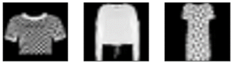
(a)

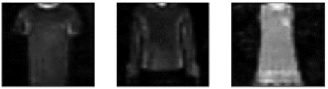
(b)

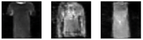
(c)

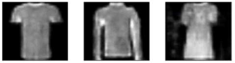
(d)

Figure 4: Samples of T-shirt, Pullover, and Dress from (a) actual images, (b) generated images from Variant 1, (c) generated images from Variant 2, and (d) generated images from Variant 3 (Proposed method).

Beyond the image quality and FID score, Fig. 5 shows the effectiveness of the generated samples from the proposed method based on the comparison between the feature of generated and actual samples. Specifically, Fig. 5 represents the t-distributed Stochastic Neighbourhood Embedding (t-SNE) of the feature from the intermediate layer of the classifier in the proposed method. t-SNE is a tool for visualizing high-dimensional data (Dimitriadis et al., 2018).

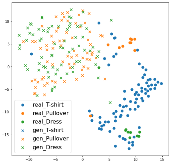
(a)

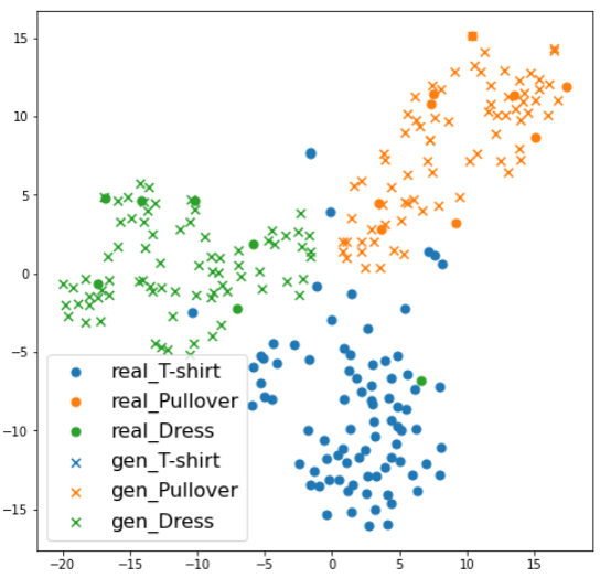
(b)

Figure 5: t-SNE of the feature from the intermediate layer of the classifier from the proposed method in epochs (a) 0 and (b) 300.

It is a nonlinear dimensionality reduction technique suitable for incorporating high-dimensional data into lower-dimensional data (2-D or 3-D) for visualization. ‘$\bullet$’ and ‘$\times$’ in Fig. 5 denote the feature in the intermediate layer of classifiers from actual and the generated samples in the balanced training batch, respectively. For a balanced training batch, the minority class has many ‘$\times$’ in each batch. Fig. 5 (a) shows the distribution alignments of actual and generated samples are different at epoch 0. Since the proposed method learns to generate realistic and distinctive samples for the classifier, Fig. 5 (b) shows that the features of generated samples (‘$\times$’) correctly follow those of actual samples (‘$\bullet$’) according to their respective labels at epoch 300. In addition, features from each label are clearly separated. The balanced training data with these properties let the proposed method achieve high classification performance.

4.2 Open-Source Data Case Studies

The open-source image data set is used for the comparative studies in this section. MNIST fashion (Xiao et al., 2017) and CIFAR-10 (Recht et al., 2018), which are widely used for the evaluation of image-based classifiers, are selected. In MNIST fashion data, five labels related to upper clothes are selected for analysis. This step provides high similarity among the classes to make a challenging problem (Choi et al., 2021). For CIFAR-10 data, Airplane, Automobile, and Ship images are selected for the same reason as the MNIST fashion data. In each label of MNIST fashion and CIFAR-10 data, 1000 and 1500 images are collected, respectively. Then, imbalanced training data is provided in Table 3. The balanced ratios are determined as 0.10 and 0.30 for MNIST fashion and CIFAR-10 data, respectively. This is because the balanced ratios with less than these values provide poor performance that is meaningless for the comparison. The remaining data sets are used as testing data.

Table 3: Imbalanced training data samples in open-source data case studies.

Data Set	Majority Class	Minority Class	Balanced Ratio	Majority Class Training Samples	Minority Class Training Samples
MNIST fashion	T-shirt	Pullover, Dress, Coat, Shirt	0.10	800	80
CIFAR-10	Airplane	Automobile, Ship	0.30	1000	300

Table 4 shows the performance evaluation of the proposed and benchmark methods in two open-source data sets. The proposed method achieves the best performance in most measures in both data sets. Compared to a baseline using imbalanced training data to train the classifier, the sampling-based method such as SMOTE (Chawla et al., 2002), B-SMOTE (Han et al., 2005), and ADASYN (He et al., 2008) generally achieves similar or worse performance.

Table 4: Performance evaluation in open-source data case studies.

	MNIST fashion			CIFAR-10
	F-score	Precision	Recall	F-score	Precision	Recall
Baseline	0.621	0.650	0.696	0.617	0.661	0.670
SMOTE	0.612	0.645	0.687	0.618	0.660	0.669
B-SMOTE	0.610	0.643	0.683	0.642	0.642	0.631
ADASYN	0.604	0.639	0.679	0.559	0.638	0.627
CDRAGAN	0.632	0.657	0.703	0.597	0.648	0.655
BAGAN-GP	0.634	0.661	0.708	0.634	0.664	0.680
Cooperative GAN	0.619	0.646	0.693	0.619	0.628	0.656
Proposed	0.642	0.664	0.713	0.652	0.655	0.684

Since both case studies have a small number of minority data, the sampling-based method has limitations in generating various data that can cover the testing data. In contrast, the GAN-based techniques usually achieve better performance than sampling-based methods since their generators learn the actual distribution and produce various training data for the classifier. Especially, the generator from the proposed method provides more diverse and better quality images by jointly optimizing the classifier, resulting in improvements in classification results.

4.3 Polymer Additive Manufacturing Process Data Case Studies

A Hyrel System 30M 3-D printer equipped with a 0.5 mm extruder nozzle is used for this case study. Fig. 6 (a) shows a front view of the printer. Acrylonitrile butadiene styrene (ABS), with a diameter of 1.75 mm, is used as a filament for printing. This study uses a digital microscope camera for high-quality image acquisition at a sampling frequency of 1 Hz. The camera is mounted near the extruder to collect images of the surface that is being printed (Fig. 6 (b)).

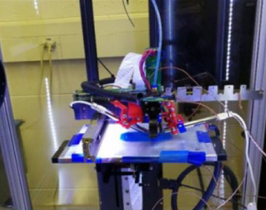
(a)

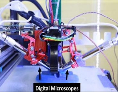
(b)

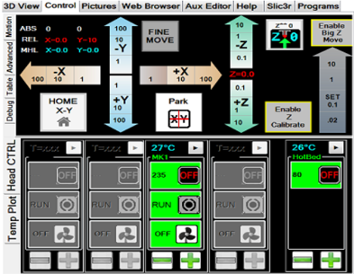
(c)

Figure 6: (a) Front view of Hyrel system 30M; (b) Digital Microscope Camera; (c) Software Controller.

Based on the design of experiments in Liu et al. (2019), the surface images for normal state, under-fill caused by feed rate and under-fill caused by the cooling fan, as shown in Fig. 7, can be obtained by setting up the specific machine parameters in the software controller (Fig. 6 (c)).

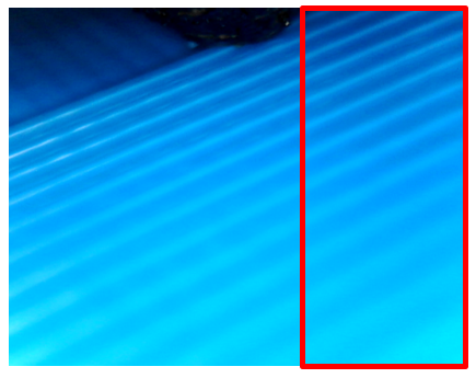
(a)

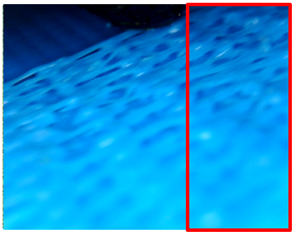
(b)

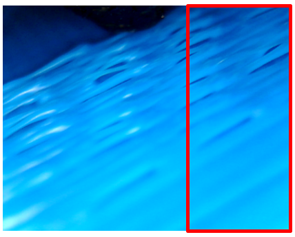
(c)

Figure 7: (a) Normal; (b) Under-fill caused by feed rate; (c) Under-fill caused by a cooling fan. The red rectangle represents the regions of interest in each image.

Two process states which are the under-fill caused by feed rate and under-fill caused by the cooling fan, are the abnormal states that cause quality deterioration in the FFF process (Liu et al., 2019; Shen et al., 2020). To increase the size of image samples, the region of interest is one-third of each image in Fig. 7 with the size of 460 $\times$ 213 $\times$ 3. Therefore, each image collected from a microscope provides three image samples. In total, there are 915 samples from the normal process state and 591 and 459 samples from under-fill caused by feed rate and cooling fan, respectively. This section provides case studies with various balanced ratios between normal and abnormal states of the FFF process to see the performance change according to ratio changes. The balanced ratios of training data are provided in Table 5, where the minority classes are denoted as the cause of abnormal states in the process. Specifically, the balanced ratios provide the performances of F-score, Precision, and Recall that are applicable in practice are utilized. The remaining images in each process state are used as testing data.

Table 5: Imbalanced training data samples in Polymer AM case studies.

Majority Class	Minority Class	Balanced Ratio	Majority Class Training Samples	Minority Class Training Samples
Normal	Under-feed, Under-fan	0.10	800	80
Normal	Under-feed, Under-fan	0.15	800	120
Normal	Under-feed, Under-fan	0.20	800	160

Fig. 8 shows the performance evaluation of the proposed and benchmark methods in various balanced ratios.

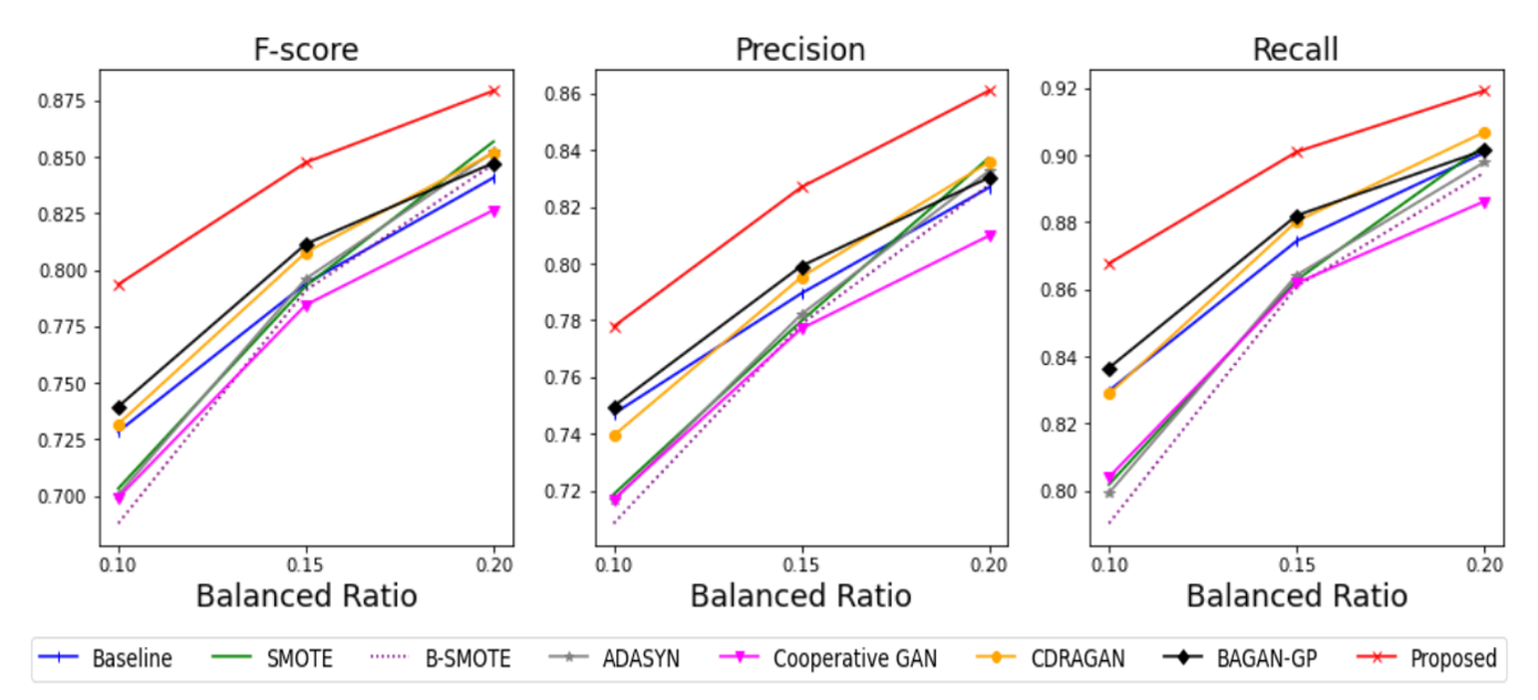
Figure 8: F-scores, precisions, and Recalls in FFF process case studies under different balanced ratios.

The performances of all the methods are improved when the number of training samples in minority classes increases (i.e., the balanced ratio increases). This is because a large number of samples provides more information for the generator to learn the actual distribution. In every balanced ratio, the proposed method achieves the best performance in all the measures, which shows the effectiveness of the realistic and state-distinguishable generated samples in the AM process. Specifically, the proposed method improved 3%$\sim$13%, 3%$\sim$10%, and 2%$\sim$10% of the performance of the benchmark methods regarding their F-score, Precision, and Recall, respectively. In addition, the proposed method performs better than cooperative GAN, which also jointly optimizes GAN and classifier but follows the basic objective function of the discriminator in GAN. This demonstrates the effectiveness of stable learning through regularizing the gradient of the discriminator and an additional task provided to the discriminator in the proposed method. Sampling-based methods show worse performance than GAN-based methods in general since the methods only consider the local information resulting in limited diverse generated images (Douzas and Bacao, 2018).

Fig. 9 shows the t-SNE of the feature from the intermediate layer of classifiers from the proposed method in epochs 0 and 300 when the balanced ratio is 0.20. Like Fig. 5, ‘$\bullet$’ and ‘$\times$’ represent features of actual and generated samples, respectively. The colors differentiate each process state in the FFF process.

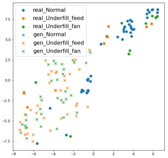
(a)

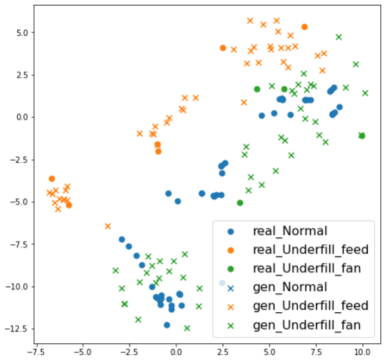
(b)

Figure 9: t-SNE of the feature from the intermediate layer of classifiers from the proposed method in epochs (a) 0 and (b) 300 in the FFF process when the balanced ratio is 0.2.

To make a balanced training data, two abnormal states in the FFF process have adequate generated samples (‘$\times$’) than actual samples (‘$\bullet$’) in each batch. Compared to epoch 0 (Fig. 9 (a)), features in epoch 300 (Fig. 9 (b)) show that the features from generated samples (‘$\times$’) of abnormal states of the FFF process follow those of actual samples (‘$\bullet$’) correctly to each process state. Based on these balanced training data in the FFF process, the classifier achieves the best prediction results compared to benchmark methods. Fig. 10 shows the samples of actual and generated images denoted as ‘$\bullet$’ and ‘$\times$’ in Fig. 9 (b), respectively. The generated images (Fig. 10 (b)) are realistic and distinguishable among process states based on both adversarial and cooperative learning in the proposed method.

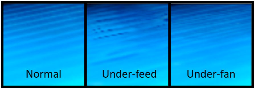
(a)

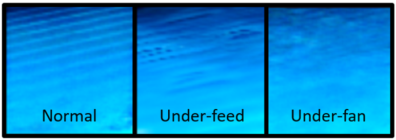
(b)

Figure 10: Samples of each process state in the FFF process from (a) actual; (b) generator when the balanced ratio is 0.2.

4.4 Metal Additive Manufacturing Process Data Case Studies

The machine ARCAMQ10 plus is utilized to print samples from the EBM process using Ti-6A1-4V powder. The dimensions of the printed sample are 15 mm $\times$ 15 mm $\times$ 25 mm. In the EBM process, there exist three different scan strategies, i.e., Dehoff, Raster, and Random (Kirka et al., 2017). The different scan strategies provide different surface patterns for the printed samples. After printing three different samples with each scan strategy, a 3-D scanner captures detailed 3-D information about the top surface (15 mm $\times$ 15 mm) quality (Wang et al., 2021). The images shown in Fig. 11 are the surface patterns of the Raster, Dehoff, and Random, respectively.

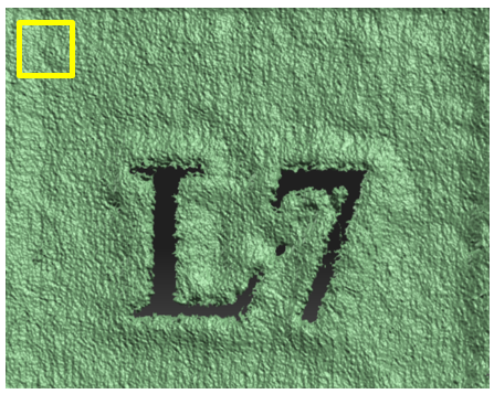
(a)

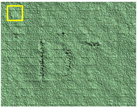
(b)

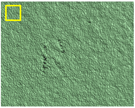
(c)

Figure 11: (a) Raster. (b) Dehoff. (c) Random; L7, D7, and R are the markers to identify samples using different scan strategies. The yellow square indicates the region of interest.

The objective of classification in this case study is to identify the scan strategy from the surface images. For each image in Fig. 11, the size is 824 $\times$ 1118 $\times$ 3. To obtain training samples, 322 images with sizes of 120 by 120 are collected from the upper part of each image (300 $\times$ 1118 $\times$ 3) since the bottom parts of the surface image with letters and numbers have many defects, such as porosity. Specifically, the collected images are highly overlapped in the horizontal directions (114 pixels) to have plenty of samples. Since the Raster scan strategy is commonly used and similar to the common AM bi-directional path, the strategy is considered a majority class (Saville et al., 2021; Nandwana and Lee, 2020). Therefore, the scan strategies with Dehoff and Random are determined as minority classes in these case studies. From the 322 images from each scan strategy, the various balanced ratios of training data are designed as in Table 6. As with polymer AM case studies in Section 4.3, the balanced ratios that provide the reasonable F-score, Precision, and Recall applicable in practice are utilized in case studies. The remaining images in each scan strategy are used as testing data.

Table 6: Imbalanced training data samples in Metal AM case studies.

Majority Class	Minority Class	Balanced Ratio	Majority Class Training Samples	Minority Class Training Samples
Raster	Dehoff, Random	0.3	150	45
Raster	Dehoff, Random	0.4	150	50
Raster	Dehoff, Random	0.5	150	75

Fig. 12 shows the performance evaluation of the proposed and benchmark methods in the EBM process. In this case study, most sampling-based methods perform better than the baseline, but the GAN-based methods usually represent worse results than the baseline. This might be caused by the highly overlapped actual samples. Compared to the polymer AM case study, the number of actual images is small and highly overlapped since we only have a single image of the top surface.

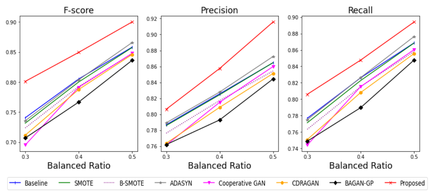
Figure 12: F-scores, Precisions, and Recalls in EBM process case studies under different balanced ratios.

Therefore, it does not provide enough information for the GAN-based methods to learn the actual distribution. Relatively, the sampling-based methods show better performance because the actual images are highly overlapped with each other. Still, the proposed method achieves the best results compared to benchmark methods by generating balanced training samples that are both realistic and scan strategy-distinguishable. Specifically, the F-score, Precision, and Recall of the proposed method were improved 4%$\sim$15%, 2%$\sim$8%, and 3%$\sim$8% over those of benchmark methods, respectively.

t-SNE results in Fig. 13 show similar results to the FFF process in Fig. 9. In epoch 300, the features from generated samples follow those of corresponding scan strategies from actual samples. Fig. 14 shows the actual and generated samples of all the scan strategies from the proposed method denoted as ‘$\bullet$’ and ‘$\times$’ in Fig. 13 (b), respectively. Compared to the actual images in Fig. 14 (a), the generated images in the EBM process (Fig. 14 (b)) are realistic. In addition, the generated images are distinguishable according to each scan strategy, which is validated by the superior classification performance of the proposed method.

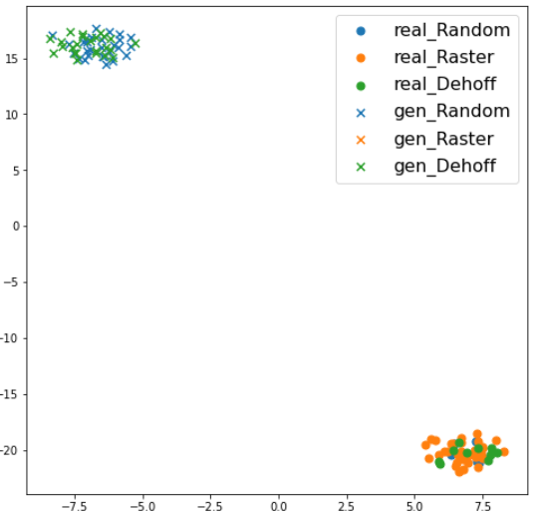
(a)

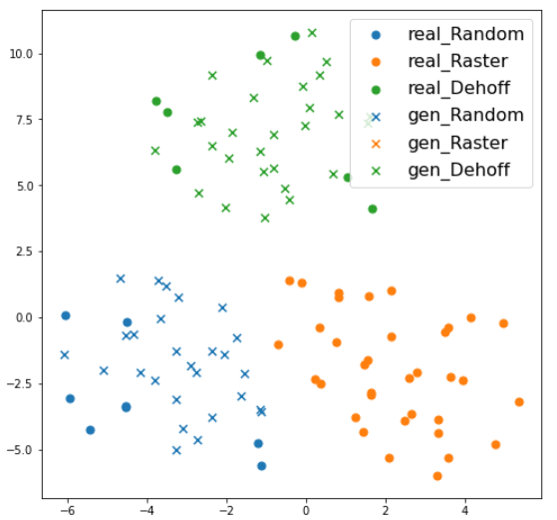
(b)

Figure 13: t-SNE of the feature from the intermediate layer of classifiers from the proposed method in epochs (a) 0 and (b) 300 in the EBM process when the balanced ratio is 0.3.

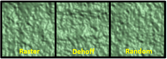
(a)

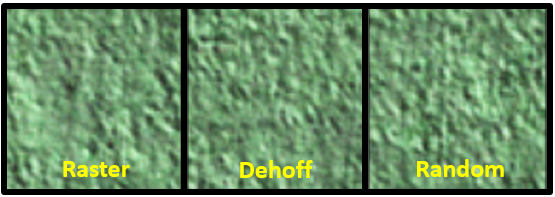
(b)

Figure 14: Samples of each scan strategy in the EBM process from (a) actual; (b) generator when balanced ratio is 0.3.

5 Conclusions

This paper proposes a novel GAN-based data augmentation method to deal with the imbalanced training data issue in manufacturing processes. The method consists of three-player, namely, generator, discriminator, and classifier, jointly optimized. Through the adversarial learning between the generator and the discriminator, the generator generates realistic samples of abnormal states in the manufacturing process. At the same time, the cooperative learning between the generator and classifier enables the generator to generate the state-distinguishable samples of the manufacturing process. The generated samples are added to actual samples and provided as a balanced training batch for a classifier. In addition, the method regularizes the gradient of the discriminator and provides an additional task to the discriminator compared to standard GAN. It prevents the gradient exploding of the generator resulting in a better quality of generated samples. The iterative learning process among these three players finally provides a classifier with high performance in classification results. The effectiveness of the proposed method is validated in both open-source and actual AM process data. Specifically, the method achieves the best performance compared to benchmark methods in the various balanced ratio of training data between normal and abnormal states in both the FFF and EBM processes.

Acknowledgments The research reported in this publication was supported by the Office of Naval Research under award N00014-18–1-2794, and the Department of Defense under award N00014-19–1-2728.

Appendix A Structure and Hyperparameters in the Methods

In this section, the detailed structure and hyperparameters of the proposed and benchmark methods are provided. Table 7 provides the hyperparameters of each method.

Table 7: Hyperparameters of each method.

Methods	Parameters	Value
SMOTE, ADASYN	Nearest K samples	5
B-SMOTE	Type	1
	Nearest K samples	5
CDRAGAN BAGAN-GP Cooperative GAN Proposed	Number of iterations	300
	Training ratio between generator and discriminator	10
	Optimizer	Adam
	Learning rate	0.0002
	Momentum	$\beta_{1}=0.5,\beta_{2}=0.9$
	Hidden layers (Discriminator)	4 blocks of [Conv2D, LeakyRelu]
	Hidden layers (Generator)	4 blocks of [Conv2D-Transpose, LeakyRelu, BatchNormalization]
	Number of Kernels in each block (Discriminator)	(64,128,128,256)
	Number of Kernels in each block (Generator)	(128,128,64,Number of channel)
	Kernel sizes	(4,4)
	Strides	(2,2)
	Padding	Same
	Activation functions	LeakyRelu, Tanh
	Kernel initializer	Random Normal(sd=0.02)
	Slope of Leaky Relu	0.2
CDRAGAN, BAGAN-GP Proposed	Gradient Penalty Coefficient	10
Cooperative GAN	Range of scheduling parameter	[0.1,0.9]
BAGAN-GP, Proposed	Epochs in pre-training	300

The gradient penalty coefficient is determined as 10 as suggested by Kodali et al. (2017); Huang and Jafari (2021). The scheduling parameter in the Cooperative GAN, is searched within a specific range ([0.1, 0.9]) following the guidelines provided in the literature (Choi et al., 2021) and selected with the values that showed the best validation performance. A batch size ($m$ in Algorithm 1) varies along the number of actual samples in each case study since the proposed method is highly computationally expensive. Specifically, batch sizes are 100 in Section. 4.1, 200 & 100 in Section. 4.2, 60 in Section. 4.3, and 50 in Section. 4.4. Table 8 shows the hyperparameters of the classifier in case studies. Convolutional Neural Network is used for the classifier. For a fair comparison, all the methods use the same classifier as described in Table 8.

Table 8: Hyperparameters of the classifier.

Parameters	Value
Number of epochs	300
Optimizer	Adam
Learning rate	0.0002
Momentum	$\beta_{1}=0.5,\beta_{2}=0.9$
Hidden Layers	4 blocks of [Conv2D, LeakyRelu]
Number kernels in each block	(32,32,128,256)
Kernel sizes	(4,4)
Strides	(2,2)
Padding	Same
Activation functions	Leaky Relu, Softmax
Kernel initializer	Random Normal (sd=0.02)
Slope of Leaky Relu	0.2

References

- \bibcommenthead
- Antoniou et al. (2017) Antoniou, A., A. Storkey, and H. Edwards. 2017. Data augmentation generative adversarial networks. arXiv preprint arXiv:1711.04340 .
- Arjovsky and Bottou (2017) Arjovsky, M. and L. Bottou. 2017. Towards principled methods for training generative adversarial networks. arXiv preprint arXiv:1701.04862 .
- Banadaki et al. (2020) Banadaki, Y., N. Razaviarab, H. Fekrmandi, and S. Sharifi. 2020. Toward enabling a reliable quality monitoring system for additive manufacturing process using deep convolutional neural networks. arXiv preprint arXiv:2003.08749 .
- Batista et al. (2004) Batista, G.E., R.C. Prati, and M.C. Monard. 2004. A study of the behavior of several methods for balancing machine learning training data. ACM SIGKDD explorations newsletter 6(1): 20–29 .
- Bhat et al. (2016) Bhat, N.N., S. Dutta, T. Vashisth, S. Pal, S.K. Pal, and R. Sen. 2016. Tool condition monitoring by svm classification of machined surface images in turning. The International Journal of Advanced Manufacturing Technology 83(9): 1487–1502 .
- Chawla et al. (2002) Chawla, N.V., K.W. Bowyer, L.O. Hall, and W.P. Kegelmeyer. 2002. Smote: synthetic minority over-sampling technique. Journal of artificial intelligence research 16: 321–357 .
- Chawla et al. (2004) Chawla, N.V., N. Japkowicz, and A. Kotcz. 2004. Special issue on learning from imbalanced data sets. ACM SIGKDD explorations newsletter 6(1): 1–6 .
- Chen et al. (2021) Chen, T., Y. Cheng, Z. Gan, J. Liu, and Z. Wang. 2021. Data-efficient gan training beyond (just) augmentations: A lottery ticket perspective. Advances in Neural Information Processing Systems 34 .
- Choi et al. (2021) Choi, H.S., D. Jung, S. Kim, and S. Yoon. 2021. Imbalanced data classification via cooperative interaction between classifier and generator. IEEE Transactions on Neural Networks and Learning Systems .
- Cui et al. (2020) Cui, W., Y. Zhang, X. Zhang, L. Li, and F. Liou. 2020. Metal additive manufacturing parts inspection using convolutional neural network. Applied Sciences 10(2): 545 .
- Davenport (1951) Davenport, H. 1951. On a principle of lipschitz. Journal of the London Mathematical Society 1(3): 179–183 .
- Dhillon and Verma (2020) Dhillon, A. and G.K. Verma. 2020. Convolutional neural network: a review of models, methodologies and applications to object detection. Progress in Artificial Intelligence 9(2): 85–112 .
- Dimitriadis et al. (2018) Dimitriadis, G., J.P. Neto, and A.R. Kampff. 2018. t-sne visualization of large-scale neural recordings. Neural computation 30(7): 1750–1774 .
- Douzas and Bacao (2018) Douzas, G. and F. Bacao. 2018. Effective data generation for imbalanced learning using conditional generative adversarial networks. Expert Systems with applications 91: 464–471 .
- Dowson and Landau (1982) Dowson, D. and B. Landau. 1982. The fréchet distance between multivariate normal distributions. Journal of multivariate analysis 12(3): 450–455 .
- Fathy et al. (2020) Fathy, Y., M. Jaber, and A. Brintrup. 2020. Learning with imbalanced data in smart manufacturing: A comparative analysis. IEEE Access 9: 2734–2757 .
- Fedus et al. (2017) Fedus, W., M. Rosca, B. Lakshminarayanan, A.M. Dai, S. Mohamed, and I. Goodfellow. 2017. Many paths to equilibrium: Gans do not need to decrease a divergence at every step. arXiv preprint arXiv:1710.08446 .
- Fernández et al. (2018) Fernández, A., S. Garcia, F. Herrera, and N.V. Chawla. 2018. Smote for learning from imbalanced data: progress and challenges, marking the 15-year anniversary. Journal of artificial intelligence research 61: 863–905 .
- Gobert et al. (2019) Gobert, C., E. Arrieta, A. Belmontes, R.B. Wicker, F. Medina, and B. McWilliams 2019. Conditional generative adversarial networks for in-situ layerwise additive manufacturing data. In 2019 International Solid Freeform Fabrication Symposium. University of Texas at Austin.
- Goodfellow et al. (2014) Goodfellow, I., J. Pouget-Abadie, M. Mirza, B. Xu, D. Warde-Farley, S. Ozair, A. Courville, and Y. Bengio. 2014. Generative adversarial nets. Advances in neural information processing systems 27 .
- Gulrajani et al. (2017) Gulrajani, I., F. Ahmed, M. Arjovsky, V. Dumoulin, and A.C. Courville. 2017. Improved training of wasserstein gans. Advances in neural information processing systems 30 .
- Guo et al. (2019) Guo, J., J. Wu, Z. Sun, J. Long, and S. Zhang. 2019. Fault diagnosis of delta 3d printers using transfer support vector machine with attitude signals. IEEE Access 7: 40359–40368 .
- Hajalfadul and Baumers (2021) Hajalfadul, M. and M. Baumers. 2021. Building a quality cost model for additive manufacturing. University Of Khartoum Engineering Journal 11(1) .
- Han et al. (2005) Han, H., W.Y. Wang, and B.H. Mao 2005. Borderline-smote: a new over-sampling method in imbalanced data sets learning. In International conference on intelligent computing, pp. 878–887. Springer.
- He et al. (2008) He, H., Y. Bai, E.A. Garcia, and S. Li 2008. Adasyn: Adaptive synthetic sampling approach for imbalanced learning. In 2008 IEEE international joint conference on neural networks (IEEE world congress on computational intelligence), pp. 1322–1328. IEEE.
- Huang and Jafari (2021) Huang, G. and A.H. Jafari. 2021. Enhanced balancing gan: Minority-class image generation. Neural Computing and Applications: 1–10 .
- Jia et al. (2019) Jia, Z., Z. Liu, C.M. Vong, and M. Pecht. 2019. A rotating machinery fault diagnosis method based on feature learning of thermal images. Ieee Access 7: 12348–12359 .
- Jin et al. (2019) Jin, Z., Z. Zhang, and G.X. Gu. 2019. Autonomous in-situ correction of fused deposition modeling printers using computer vision and deep learning. Manufacturing Letters 22: 11–15 .
- Kingma and Ba (2014) Kingma, D.P. and J. Ba. 2014. Adam: A method for stochastic optimization. arXiv preprint arXiv:1412.6980 .
- Kirka et al. (2017) Kirka, M.M., Y. Lee, D.A. Greeley, A. Okello, M.J. Goin, M.T. Pearce, and R.R. Dehoff. 2017. Strategy for texture management in metals additive manufacturing. Jom 69(3): 523–531 .
- Kiyasseh et al. (2020) Kiyasseh, D., G.A. Tadesse, L. Thwaites, T. Zhu, D. Clifton, et al. 2020. Plethaugment: Gan-based ppg augmentation for medical diagnosis in low-resource settings. IEEE journal of biomedical and health informatics 24(11): 3226–3235 .
- Kodali et al. (2017) Kodali, N., J. Abernethy, J. Hays, and Z. Kira. 2017. On convergence and stability of gans. arXiv preprint arXiv:1705.07215 .
- Kwon et al. (2020) Kwon, O., H.G. Kim, M.J. Ham, W. Kim, G.H. Kim, J.H. Cho, N.I. Kim, and K. Kim. 2020. A deep neural network for classification of melt-pool images in metal additive manufacturing. Journal of Intelligent Manufacturing 31(2): 375–386 .
- Kyeong and Kim (2018) Kyeong, K. and H. Kim. 2018. Classification of mixed-type defect patterns in wafer bin maps using convolutional neural networks. IEEE Transactions on Semiconductor Manufacturing 31(3): 395–402 .
- Lee et al. (2020) Lee, X.Y., S.K. Saha, S. Sarkar, and B. Giera. 2020. Automated detection of part quality during two-photon lithography via deep learning. Additive manufacturing 36: 101444 .
- Li et al. (2021) Li, Y., Z. Shi, C. Liu, W. Tian, Z. Kong, and C.B. Williams. 2021. Augmented time regularized generative adversarial network (atr-gan) for data augmentation in online process anomaly detection. IEEE Transactions on Automation Science and Engineering .
- Liu et al. (2021) Liu, C., Z. Kong, S. Babu, C. Joslin, and J. Ferguson. 2021. An integrated manifold learning approach for high-dimensional data feature extractions and its applications to online process monitoring of additive manufacturing. IISE Transactions 53(11): 1215–1230 .
- Liu et al. (2019) Liu, C., A.C.C. Law, D. Roberson, and Z.J. Kong. 2019. Image analysis-based closed loop quality control for additive manufacturing with fused filament fabrication. Journal of Manufacturing Systems 51: 75–86 .
- Mahmoudi et al. (2019) Mahmoudi, M., A.A. Ezzat, and A. Elwany. 2019. Layerwise anomaly detection in laser powder-bed fusion metal additive manufacturing. Journal of Manufacturing Science and Engineering 141(3) .
- Makes and Collaborative (2017) Makes, A. and A.A.M.S. Collaborative. 2017. Standardization roadmap for additive manufacturing. February), Public Draft .
- Mariani et al. (2018) Mariani, G., F. Scheidegger, R. Istrate, C. Bekas, and C. Malossi. 2018. Bagan: Data augmentation with balancing gan. arXiv preprint arXiv:1803.09655 .
- Mikołajczyk and Grochowski (2018) Mikołajczyk, A. and M. Grochowski 2018. Data augmentation for improving deep learning in image classification problem. In 2018 international interdisciplinary PhD workshop (IIPhDW), pp. 117–122. IEEE.
- Mirza and Osindero (2014) Mirza, M. and S. Osindero. 2014. Conditional generative adversarial nets. arXiv preprint arXiv:1411.1784 .
- Montazeri and Rao (2018) Montazeri, M. and P. Rao. 2018. Sensor-based build condition monitoring in laser powder bed fusion additive manufacturing process using a spectral graph theoretic approach. Journal of Manufacturing Science and Engineering 140(9) .
- Mycroft et al. (2020) Mycroft, W., M. Katzman, S. Tammas-Williams, E. Hernandez-Nava, G. Panoutsos, I. Todd, and V. Kadirkamanathan. 2020. A data-driven approach for predicting printability in metal additive manufacturing processes. Journal of Intelligent Manufacturing 31(7): 1769–1781 .
- Nandwana and Lee (2020) Nandwana, P. and Y. Lee. 2020. Influence of scan strategy on porosity and microstructure of ti-6al-4v fabricated by electron beam powder bed fusion. Materials Today Communications 24: 100962 .
- Odena et al. (2017) Odena, A., C. Olah, and J. Shlens 2017. Conditional image synthesis with auxiliary classifier gans. In International conference on machine learning, pp. 2642–2651. PMLR.
- Powers (2020) Powers, D.M. 2020. Evaluation: from precision, recall and f-measure to roc, informedness, markedness and correlation. arXiv preprint arXiv:2010.16061 .
- Ranasinghe and Parlikad (2019) Ranasinghe, G.D. and A.K. Parlikad 2019. Generating real-valued failure data for prognostics under the conditions of limited data availability. In 2019 IEEE International Conference on Prognostics and Health Management (ICPHM), pp. 1–8. IEEE.
- Recht et al. (2018) Recht, B., R. Roelofs, L. Schmidt, and V. Shankar. 2018. Do cifar-10 classifiers generalize to cifar-10? arXiv preprint arXiv:1806.00451 .
- Sáez et al. (2015) Sáez, J.A., J. Luengo, J. Stefanowski, and F. Herrera. 2015. Smote–ipf: Addressing the noisy and borderline examples problem in imbalanced classification by a re-sampling method with filtering. Information Sciences 291: 184–203 .
- Saville et al. (2021) Saville, A.I., S.C. Vogel, A. Creuziger, J.T. Benzing, A.L. Pilchak, P. Nandwana, J. Klemm-Toole, K.D. Clarke, S.L. Semiatin, and A.J. Clarke. 2021. Texture evolution as a function of scan strategy and build height in electron beam melted ti-6al-4v. Additive manufacturing 46: 102118 .
- Shen et al. (2020) Shen, B., W. Xie, and Z.J. Kong. 2020. Clustered discriminant regression for high-dimensional data feature extraction and its applications in healthcare and additive manufacturing. IEEE Transactions on Automation Science and Engineering 18(4): 1998–2010 .
- Shorten and Khoshgoftaar (2019) Shorten, C. and T.M. Khoshgoftaar. 2019. A survey on image data augmentation for deep learning. Journal of big data 6(1): 1–48 .
- Tao and Wang (2020) Tao, S. and J. Wang 2020. Alleviation of gradient exploding in gans: Fake can be real. In Proceedings of the IEEE/CVF Conference on Computer Vision and Pattern Recognition, pp. 1191–1200.
- Tran et al. (2018) Tran, N.T., T.A. Bui, and N.M. Cheung 2018. Dist-gan: An improved gan using distance constraints. In Proceedings of the European conference on computer vision (ECCV), pp. 370–385.
- Wang et al. (2017) Wang, C., Z. Yu, H. Zheng, N. Wang, and B. Zheng 2017. Cgan-plankton: Towards large-scale imbalanced class generation and fine-grained classification. In 2017 IEEE International Conference on Image Processing (ICIP), pp. 855–859. IEEE.
- Wang and Chen (2019) Wang, R. and N. Chen. 2019. Wafer map defect pattern recognition using rotation-invariant features. IEEE Transactions on Semiconductor Manufacturing 32(4): 596–604 .
- Wang et al. (2021) Wang, R., A.C. Law, D. Garcia, S. Yang, and Z. Kong. 2021. Development of structured light 3d-scanner with high spatial resolution and its applications for additive manufacturing quality assurance. The International Journal of Advanced Manufacturing Technology 117(3): 845–862 .
- Xiao et al. (2017) Xiao, H., K. Rasul, and R. Vollgraf. 2017. Fashion-mnist: a novel image dataset for benchmarking machine learning algorithms. arXiv preprint arXiv:1708.07747 .
- Zhang et al. (2020) Zhang, J., S. Yi, G. Liang, G. Hongli, H. Xin, and S. Hongliang. 2020. A new bearing fault diagnosis method based on modified convolutional neural networks. Chinese Journal of Aeronautics 33(2): 439–447 .
- Zhang (2018) Zhang, Y. 2018. Deep generative model for multi-class imbalanced learning. University of Rhode Island .
- Zhou et al. (2020) Zhou, L., H. Tao, W. Paszke, V. Stojanovic, and H. Yang. 2020. Pd-type iterative learning control for uncertain spatially interconnected systems. Mathematics 8(9): 1528 .
- Zhu et al. (2019) Zhu, J., G. Yang, and P. Lio 2019. How can we make gan perform better in single medical image super-resolution? a lesion focused multi-scale approach. In 2019 IEEE 16th International Symposium on Biomedical Imaging (ISBI 2019), pp. 1669–1673. IEEE.