Critical growth of cerebral tissue in organoids: theory and experiments

Abstract

We develop a Fokker-Planck theory of tissue growth with three types of cells (symmetrically dividing, asymmetrically dividing and non-dividing) as main agents to study the growth dynamics of human cerebral organoids. Fitting the theory to lineage tracing data obtained in next generation sequencing experiments, we show that the growth of cerebral organoids is a critical process. We derive analytical expressions describing the time evolution of clonal lineage sizes and show how power-law distributions arise in the limit of long times due to the vanishing of a characteristic growth scale. We discuss that the independence of critical growth on initial conditions could be biologically advantageous.

Introduction

The mechanisms of tissue growth and renewal are a core topic of stem-cell research (Chatzeli_2020_tracing_fate_stem_cells, ; Simons2011_cell_renewal_strategies, ). In particular, the role of stochasticity in cell differentiation is discussed (lin_2021_neural_progenitors_mammalian, ; zechner2020_stochasticity_differentiation, ; Klingler2020_cortical_stochastic, ; Llorca2019_stochastic_differentiation_cortex, ; Corominas2020_intestinal_niches, ; smith_2015_stochasticity_cell_diff, ). Single cell sequencing (kashima_2020_single_cell_seq_rev, ), combined with the labeling of cells with inheritable DNA sequences, enables large scale, quantitative studies of cell populations in biological tissues, where offspring populations can be traced back to their individual ancestral cells (wagner_2020_sc_omics_lineage_tracing, ; kester_2018_single_cell_lineage_tracing, ). Such lineage tracing experiments have revealed that offspring numbers in mammalian cerebral tissue can vary by several orders of magnitude (Llorca2019_stochastic_differentiation_cortex, ; esk_2020_organoid_tissue_screen, ), which supports the hypothesis that stochasticity is an important property of cell proliferation and differentiation in the developing cerebral cortex.

This work presents a study of lineage tracing data obtained by sequencing 15 cerebral organoids at different stages of their development (esk_2020_organoid_tissue_screen, ). Cerebral organoids are highly controllable, self organized in vitro models of the human cerebral cortex grown from stem cells. Organoids are unique because they model human tissues which cannot be studied in vivo. They have therefore become important biological tools to study neural development and brain diseases (lancaster2013_organoids, ; lancaster2017_organoids, ; kim2020human, ). We take a physics point of view on the population dynamics of cell lineages in cerebral organoids, show that organoid growth is a critical process, and discuss the biological implications.

Figure 1: The SAN model of dividing and differentiating cells. Stem cells (green, S) either divide at rate $g_{S}$ (S$\rightarrow$2S), differentiate at rate $g_{A}$ (S$\rightarrow$A) or die at a rate $g_{0}$ (S$\rightarrow$Ø). Differentiated cells (orange, A) that committed to a developmental trajectory either divide asymmetrically (A$\rightarrow$A+N) at a rate $g_{A}$, or differentiate directly into non-dividing N cells (rate $g_{F}$). On average, each A cell produces $\bar{N}$ N-cells until it looses the ability to divide. At criticality, the rates $g_{S}$ (division) and $g_{A}$ (differentiation) are equal.

Model

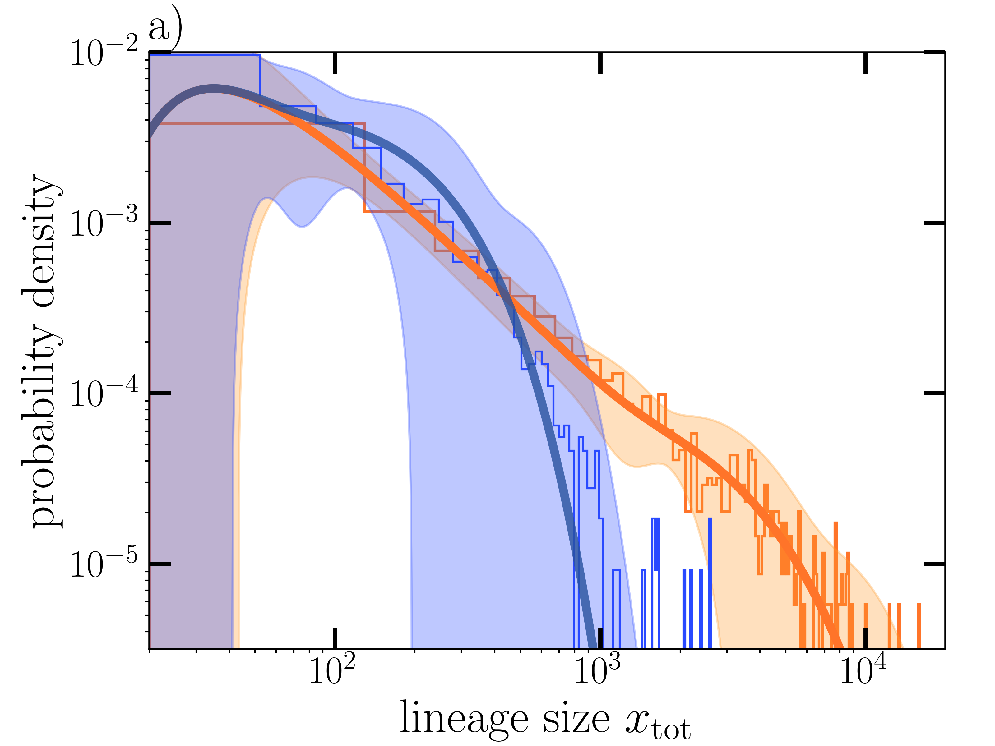
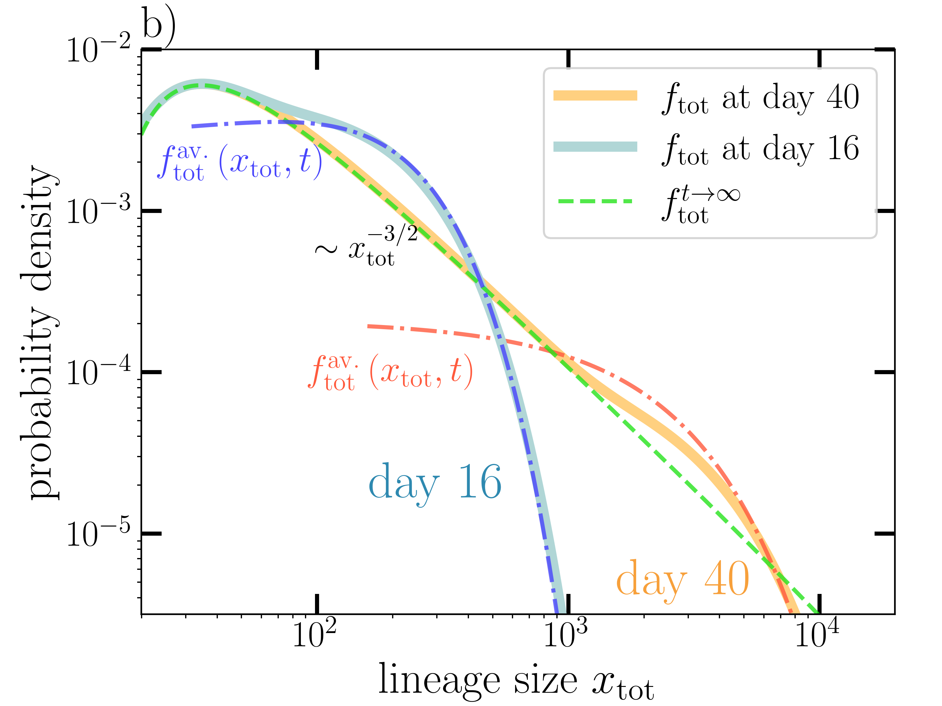
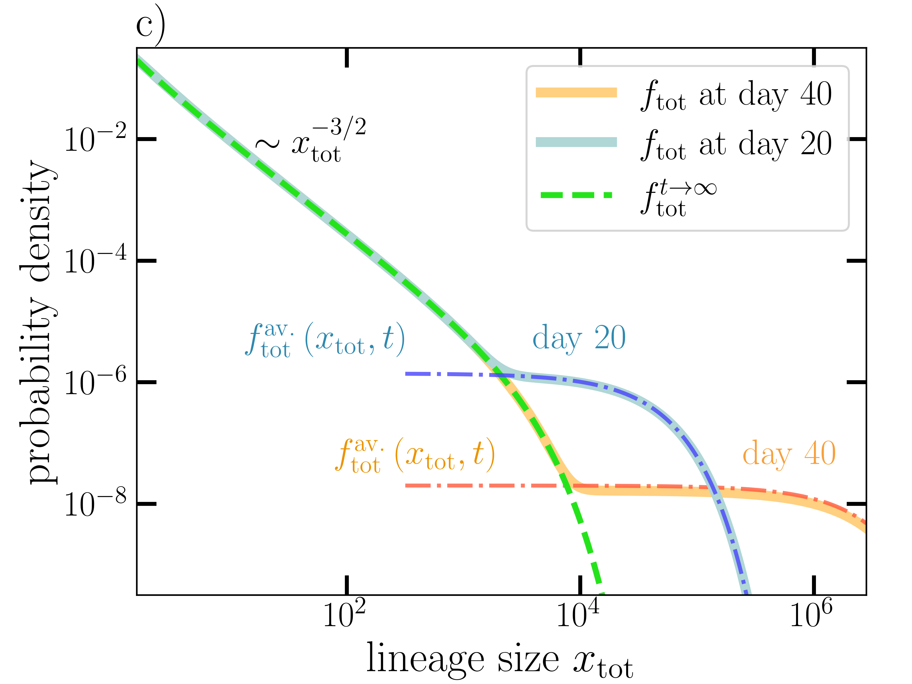
Figure 2: a) Histograms of lineage sizes of two organoids sequenced at $t=16\,\mathrm{days}$ (blue) and $t=40\,\mathrm{days}$ (orange) and the corresponding probability densities of the SAN model $f_{\mathrm{tot}}\left(x_{\mathrm{tot}},t\right)$ (thick solid lines). Parameter values are given in Table 1. Shaded areas indicate error margnis. b) Theoretical SAN model probability densities and the analytical approximations $f_{\mathrm{tot}}^{t\rightarrow\infty}\left(x_{\mathrm{tot}}\right)$ (dashed, green line) and $f_{\mathrm{tot}}^{\mathrm{av.}}\left(x_{\mathrm{tot}},t\right)$ (dashed, dotted lines) of Eqs. (5), (6) for the parameter estimates of Table 1 ($\alpha<0$ - sub-critical regime). For $t\rightarrow\infty$ the distribution approaches the weakly truncated $3/2$-power-law Lévy distribution $f_{\mathrm{tot}}^{t\rightarrow\infty}\left(x_{\mathrm{tot}}\right)$ everywhere. c) SAN model predictions for small $\alpha>0$ (super-critical regime). $f_{\mathrm{tot}}\left(x_{\mathrm{tot}},t\right)$ still approaches $f_{\mathrm{tot}}^{t\rightarrow\infty}\left(x_{\mathrm{tot}}\right)$, except for very large lineage sizes, where the avalanche of active S-cell proliferation dominates. We used $\alpha=0.2$, $\beta=10$, $s_{0}=1$ and $N=1$.

Our study begins with the observation that the numbers of descendants of an individual stem cell in the organoid (lineage sizes) are roughly distributed according to a 3/2-power-law. This behavior becomes more and more pronounced at late stages of the organoid development. To model the growth process mathematically, we build upon the theory of continuous state branching processes (feller1951_Two_singular_diffusion_problems, ; lamperti1967limit, ), pioneered by Feller (Feller_Kampf_ums_Dasein, ). These processes are known to lead to power-law distributed poluation sizes (Zapperi1995_SOC, ; alava2012branching, ; diSanto_munoz_2017branching, ).

We thus introduce the SAN model. It consists of three agents: symmetrically dividing S-cells that represent stem cells, asymmetrically dividing A-cells and non-dividing N-cells (fully developed cells, e.g. neurons). S-cells undergo symmetric division (S$\rightarrow$2S) at rate $g_{S}$, differentiation (S$\rightarrow$A) at rate $g_{A}$ and death (S$\rightarrow$0) at rate $g_{0}$. A-cells have committed to a developmental trajectory and produce N-cells through asymmetric divisions (A$\rightarrow$A+N) at a rate $g_{N}$ until the process is terminated by direct differentiation (A$\rightarrow$N) (rate $g_{F}$). The branching process of symmetric division and differentiation of S-cells with rates $g_{S}$ and $g_{A}$ is at the heart of the SAN-model. Criticality is reached, when the two rates are equal: $g_{S}=g_{A}$. The model is illustrated in Fig. 1. We solve the SAN-model analytically in the continuum limit and show how, at long times, $3/2$-power-law distributions of cell populations asymptotically arise near criticality. Fitting the model predictions to the empirical data of Ref. (esk_2020_organoid_tissue_screen, ), we show that cerebral organoid growth is indeed critical (see Fig. 2 and Table 1).

In experiments, organoids are grown for forty days. As we will demonstrate, our model can describe tissue growth as a dynamical process with a limited number of parameters – three rates and one initial condition.

Fokker-Planck description of lineage dynamics

We start with a master equation for the SAN process. Individual populations of S, A and N-cells are not accessible in experiments, since all descendants of a stem cell inherit the same lineage identifier. We therefore need to calculate the probability distribution of the total lineage size $x_{\mathrm{tot}}=s+a+n$. This calls for a slight simplification. We replace the processes A$\rightarrow$A + N and A$\rightarrow$N by the assumption that each A-cell produces $\bar{N}=1+g_{N}/g_{F}$ N-cells over the course of its existence (where the $+1$ stems from the final A$\rightarrow$N conversion) (Fig. 1). Since the N-cell output per A-cell varies by multiple orders of magnitude less than the total offspring of an S-cell (pflug2021_SAN, ), this simplification does not affect the model’s main predictions, making it analytically tractable. $\bar{N}$ is a fitting parameter in our theory. The total lineage size becomes $x_{\mathrm{tot}}=s+n$. The master equation for the probability distribution $f$ of S- and N-cell numbers $s$, $n$ at time $t$ then reads

$$\partial_{t}f\left(s,n,t\right) = g_{S}\left(s-1\right)f\left(s-1,n,t\right)$$ (1)

$$+ g_{A}\left(s+1\right)f\left(s+1,n-\bar{N},t\right)$$

$$+ g_{0}\left(s+1\right)f\left(s+1,n,t\right)$$

$$- \left(g_{S}s+g_{A}s+g_{0}s\right)f\left(s,n,t\right).$$

The right hand side terms of Eq. (1) correspond to the different processes that the cells undergo: S-cell death at rate $g_{0}$, S-cell division at rate $g_{S}$ and differentiation into $\bar{N}$ N-cells at rate $g_{A}$. Focusing on large cell counts, we translate the discrete process of Eq. (1) into a continuous version given by the Fokker-Planck equation (vanKampen, ):

$$\partial_{t}f\left(\mathbf{x},t\right)=\mathcal{L}f\left(\mathbf{x},t\right)$$ (2)

with the differential operator

$$\mathcal{L} =\left(-\alpha\partial_{s}+\frac{\beta}{2}\partial_{s}^{2}-g_{A}\bar{N}\partial_{s}\partial_{n}-\bar{N}g_{A}\partial_{n}+\frac{g_{A}\bar{N}^{2}}{2}\partial_{n}^{2}\right)s.$$ (3)

Here, $\mathbf{x}=\left(s,n\right)$ is a vector with continuous cell numbers as components, $\alpha=g_{S}-g_{A}-g_{0}$ and $\beta=g_{S}+g_{A}+g_{0}$.

Regimes of growth: power-laws and avalanches

Next, we want to examine the implications of the Fokker-Planck Eq. (2) for the lineage sizes within a tissue sample. We solve Eq. (2) with the initial condition $f\left(\mathbf{x},t=0\right)=\delta\left(s-s_{0}\right)\delta\left(n\right)$. $s_{0}$ corresponds to the initial number of stem cells of a lineage – not necessarily unity, since stem cells proliferate at initial stages of organoid preparation, which are not considered here otherwise. Using the Fourier transform of Eqs. (2), (3) with respect to $\mathbf{x}$ and the method of characteristics to solve the resulting first order partial differential equation (see supplementary material), we find the characteristic function of $f\left(\mathbf{x},t\right)$, $\tilde{f}\left(\mathbf{q},t\right)=\int_{-\infty}^{\infty}e^{-i\mathbf{q}\cdot\mathbf{x}}f\left(\mathbf{x},t\right)$.

The distribution of total lineage sizes $x_{\mathrm{tot}}$ is given by an integral of $f\left(\mathbf{x},t\right)$ over all states with equal $x_{\mathrm{tot}}$:

$$f_{\mathrm{tot}}\left(x_{\mathrm{tot}},t\right)=\int_{0}^{x_{\mathrm{tot}}}f\left(s,x_{\mathrm{tot}}-s,t\right)ds.$$ (4)

The presence of a critical point can be clearly seen from the expectation value of the stem cell population: for finite $\alpha$, $\left\langle s\right\rangle=s_{0}e^{\alpha t}$, whereas for the critical $\alpha=0$, $\left\langle s\right\rangle=s_{0}$. For $t\rightarrow\infty$, $f_{\mathrm{tot}}\left(x_{\mathrm{tot}},t\right)$ approaches a limiting distribution $f_{\mathrm{tot}}^{t\rightarrow\infty}\left(x_{\mathrm{tot}}\right)$ – a truncated $3/2$-power-law Lévy distribution (tsallis1997levy, ; gnedenko1954_stable_distr, ; bouchaud1990anomalous, ):

$$f_{\mathrm{tot}}^{t\rightarrow\infty}\left(x_{\mathrm{tot}}\right)\approx\frac{s_{0}\beta e^{-\frac{\alpha^{2}x_{\mathrm{tot}}}{\beta^{2}\bar{N}}}}{2\sqrt{2\pi}\bar{N}\left(x_{\mathrm{tot}}/\bar{N}\right)^{3/2}}.$$ (5)

This formula holds for $\alpha\ll\beta$. For a more general expression see supplemetary Eq. (S 28). At criticality the distribution becomes a true $3/2$-power-law.

The way in which $f_{\mathrm{tot}}\left(x_{\mathrm{tot}},t\right)$ approaches the limit of Eq. (5) is very different for $\alpha>0$ and $\alpha<0$. For positive $\alpha$ and large enough lineage size $x_{\mathrm{tot}}>x_{\mathrm{tot}}^{*}\sim e^{\alpha t}$, there is a region where $f_{\mathrm{tot}}\left(x_{\mathrm{tot}},t\right)$ is not approximated by Eq. (5). This is the avalanche region illustrated in Fig. 2 c). Here, lineages have a high percentage of proliferating S-cells which are driving the system’s growth. The lineage sizes are very large but the probability of their occurrence is very small. For $x_{\mathrm{tot}}<x_{\mathrm{tot}}^{*}$ most lineages are fully differentiated and stopped growing. In the avalanche regime, $f_{\mathrm{tot}}\left(x_{\mathrm{tot}},t\right)$ can be approximated by

$$f_{\mathrm{tot}}^{\mathrm{av.}}\left(x_{\mathrm{tot}},t\right)\approx\frac{\sqrt{a}\exp\left(-\frac{a}{q_{\mathrm{tot}}^{*}}-\frac{x_{\mathrm{tot}}}{q_{\mathrm{tot}}^{*}N}\right)}{q_{\mathrm{tot}}^{*}\sqrt{x_{\mathrm{tot}}\bar{N}}}I_{1}\left(2\sqrt{\frac{ax_{\mathrm{tot}}}{q_{\mathrm{tot}}^{*2}\bar{N}}}\right)$$ (6)

where $I_{1}\left(z\right)$ is the modified Bessel function of the first kind and $q_{\mathrm{tot}}^{*}\left(t\right)$ and $a\left(t\right)$ are defined in supplementary Eqs. (S 37) and (S 42).

For $\alpha<0$, we also find an avalanche region with an active S-cell population approximately described by Eq. (6) (even though the avalanche will stop eventually). As pointed out in the supplement, the approximation breaks down for $\alpha t>1$, but is still reasonable for the data at hand. This region is located at large $x_{\mathrm{tot}}$, for which $f_{\mathrm{tot}}\left(x_{\mathrm{tot}},t\right)>f_{\mathrm{tot}}^{t\rightarrow\infty}\left(x_{\mathrm{tot}}\right)$, followed by a rapid truncation at even larger $x_{\mathrm{tot}}$ (Fig. 2 b)). In contrast to the behavior at $\alpha>0$, $f_{\mathrm{tot}}\left(x_{\mathrm{tot}},t\right)$ convergences to $f_{\mathrm{tot}}^{t\rightarrow\infty}\left(x_{\mathrm{tot}}\right)$ uniformly: the avalanches becomes less and less pronounced as $t\rightarrow\infty$, because the S-cells of all lineages eventually fully differentiate if $\alpha\leq 0$ (Feller_Kampf_ums_Dasein, ). Our analysis of the data shows that $\alpha\lesssim 0$ holds in experiments (see Table 1).

Dynamics and criticality in experiments

The experimental data consists of lineage identifier counts for 15 organoids that were sequenced on days 16, 21, 25, 32 and 40 – three copies for each day(esk_2020_organoid_tissue_screen, ). Accounting for statistical and readout errors, they can be related to lineage sizes (pflug2021_SAN, ). Each organoid consists of $\sim 10^{4}$ lineages, while total cell counts evolve from $\sim 10^{5}$ at day 16 to $\sim 10^{6}$ at day 40. The organoids grow undisturbed from day 11 onward, when they are not subjected to intrusive procedures anymore. Four parameters are determined from experimental data: $\alpha$, $\beta$, $s_{0}$ and $\bar{N}$. The data at day 40 is very roughly distributed according to an $x^{-3/2}$ power-law (see Fig. 2), indicating near critical growth with $\alpha\ll\beta$.

To determine the parameters precisely, we use the empirical characteristic function of the data

$$\tilde{f}_{\mathrm{exp}}\left(q_{\mathrm{tot}}\right)=\sum_{k}e^{iq_{\mathrm{tot}}x_{\mathrm{tot}}^{\left(k\right)}}.$$ (7)

Here $x_{\mathrm{tot}}^{\left(i\right)}$ are the experimentally determined lineage sizes. The characteristic function of our model $\tilde{f}\left(q_{\mathrm{tot}},t\right)$ (Eq. (S 33)) is then least squares fitted to $\tilde{f}_{\mathrm{exp}}\left(q_{\mathrm{tot}}\right)$. Moving the fitting procedure to Fourier space has several advantages: $\tilde{f}_{\mathrm{exp}}\left(q_{\mathrm{tot}}\right)$ is less noisy than the empirical probability distribution and no smoothing procedures such as kernel density estimates need to be used. Approximations needed when transforming $\tilde{f}\left(q_{\mathrm{tot}},t\right)$ to real space are avoided. Model fitting via the characteristic function has been considered e.g. in Refs. (yu2004_characteristic_function_fitting, ; chan2009_characteristic_function_fitting, ). Our estimates for the model parameters are shown in Table 1.

$\alpha\left[\mathrm{day}^{-1}\right]$	$-0.018\pm 0.004$
$\beta\left[\mathrm{day}^{-1}\right]$	$4\pm 1$
$s_{0}$	$9\pm 3$
$\bar{N}$	$2\pm 1$

Table 1: Parameters of the SAN model estimated from experimental data with one standard deviation errors. $\alpha$ is the net growth rate of the stem cell population, and $\beta$ characterizes the stochasticity of the system. $s_{0}$ and $\bar{N}$ are the average initial number of stem cells and the average number of N-cells produced by each stem cell, respectively.

In Fig. 2 a) we show a comparison between the probability densities of the SAN model $f_{\mathrm{tot}}\left(x_{\mathrm{tot}},t\right)$ and binned histograms of the data at days 16 and 40. We used 500 bins for the data at day 40, and 80 bins for day 16. In the supplement, we show that the agreement is independent on bin-size. Small lineages ($<20$ cells) were excluded since these lineages, with a high probability, died out at preparatory stages. $f_{\mathrm{tot}}\left(x_{\mathrm{tot}},t\right)$ is found using a Fast Fourier Transform of $\tilde{f}\left(q_{\mathrm{tot}},t\right)$.

The estimates of Table 1 show that organoid growth is indeed a critical process with $\left|\alpha\right|\ll\beta$. It also shows that even at day $40$ the process is far from its $t\rightarrow\infty$ limit ($\alpha t\approx 0.8$) and the organoids maintain an avalanche-like population of S-cells at large $x_{\mathrm{tot}}$.

The SAN model is only a minimal model of biological reality and as such cannot account for the full spread of the experimental data. It does, for example, not account for the data at small $x_{\mathrm{tot}}$ (see Fig. 2). Many small lineages have died out in the early stages of the organoid development and are obviously not described by SAN dynamics. We assumed that all lineages consist of $s_{0}$ stem cells at day 11. This is only an average. While for large lineages the initial number of stem cells is unimportant since the growth is stochastic, it matters for lineages that differentiated quickly. Other neglected aspects are the time dependence of rates, and the non-markovian nature of division and differentiation. Despite these caveats, the SAN model proves to be surprisingly robust and fits the experimental data well. In supplementary section D, we perform Kolmogorov-Smirnov (K-S) tests on different intervals for the data at day 40. K-S tests are a sensitive tool to test the power-law behavior of empirical data (clauset2009power-law_Kolmogorov_Smirnov, ; touboul2010power_law_neural_avalanches_Kolmogorov_Smirnov, ; touboul2017power_law_neural_avalanches_Kolmogorov_Smirnov, ). We find that the test produces high p-values (up to $p\approx 0.8$) in the region between $x_{\mathrm{tot}}\approx 200$ and $x_{\mathrm{tot}}\approx 2000$, where the power-law is most pronounced.

Extinction trajectories

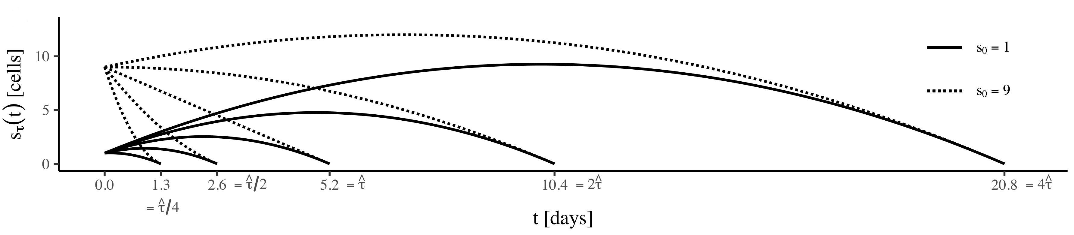
Figure 3: Single lineage stem cell populations for initial sizes $s_{0}=1$ (solid lines) and $s_{0}=9$ (dotted lines) and different extinction times $\tau$ (see Eq. (9)). For large extinction times $\tau$, the trajectories for $s_{0}=1$ and $s_{0}=9$ become equal for large times: In the critical state the population dynamics is dominated by stochasticity, and hence obtains a universal form independent of the initial conditions.

We now turn to the influence of criticality on the dynamics of single lineages. We focus on $\alpha=0$ and restrict ourselves to S-cells as the only dynamical component. Neglecting the dynamics of the $n$ variable, we drop all but the first two terms in $\mathcal{L}$ in Eq. (3). The reduced Fokker-Planck equation is equivalent to the stochastic differential equation

$$ds=\sqrt{{\beta s}}dw(t).$$ (8)

$w\left(t\right)$ is the standard Brownian motion. It is known that any $s\left(t\right)$ described by Eq. (8), at some time $\tau$, reaches $s\left(\tau\right)=0$ (Feller_Kampf_ums_Dasein, ), i.e. the S-cell population of the lineage goes extinct due to differentiation. Using the Onsager-Machlup formalism (durr_onsager-machlup_1978, ), we find the extinction trajectory

$$s_{\tau}\left(t\right)=s_{0}\left(1-\frac{1}{\tau}\right)\left(1+\left(\frac{\tau}{\hat{\tau}}-1\right)\frac{t}{\tau}\right).$$ (9)

It describes the most probable path between $s\left(0\right)=s_{0}$ and $s\left(\tau\right)=0$ (see Fig. 3). Here, $\hat{\tau}=4s_{0}/\left(\sqrt{3}\beta\right)$. Details of the calculation are given in the supplementary material. Eq. (9) and Fig 3 show that at criticality, the cells loose memory of the initial condition $s_{0}$, since for $\hat{\tau}\ll t<\tau$

$$s_{\tau}\left(t\right)\sim\sqrt{3}\beta t\left(1-t/\tau\right)/4.$$ (10)

This is not the case for $\alpha\gtrless 0$.

Most importantly, since the lineage sizes are power-law distributed, an overwhelming majority of organoid cells will belong to a few very large lineages. For these lineages, $\tau\gg\hat{\tau}$ will hold, meaning that their development will be largely independent of the initial condition $s_{0}$ (Eq. (10)). This is an essential feature of critical growth: it is independent of the initial conditions.

Discussion

Finally, we discuss possible implications of critical tissue growth. Tuning itself to the critical point, the organoid maximizes the stochasticity of the growth process. We are not dealing with stochastic growth at a given rate. Instead, the characteristic time scale of growth vanishes ($\alpha=0$) and growth is fully determined by the stochasticity of the process. This is in contrast to many other examples of organ growth and regeneration (fausto2000liver, ; zeng2008_organ_size_control, ; Ainslie2020_Drosophila_tissue_growth_kinetics, ) where the growth process is arrested in a coordinated manner. In critical growth, the long term dynamics of large lineages, which make up most of the organoid, does not depend on initial conditions. Stochastic fluctuations have erased all memory of the lineage’s initial size. This might hint at a biological advantage of the critical regime: the outcome of the growth process is less influenced by perturbations in its initial stages, when the tissue is most susceptible to disturbances.

Second, the critical nature of the process implies a mechanism balancing the rates of division and differentiation of stem cells. Such balancing mechanisms are known from homeostatic stem cell renewal (simons_strategies_2011, ). One distinguishes between mechanisms based on asymmetric division (only one daughter cell is a stem cell while the other differentiates) and population asymmetry (the rates of stem cell loss and division are balanced on population level). The first strategy cannot produce critical lineage dynamics because it is strictly deterministic. On the population level, stem cell niches are a well known regulatory mechanism for homeostatic tissues (moore2006stem, ; lin_classic_2015, ; Corominas2020_intestinal_niches, ) found in intestinal crypts (moore2006stem, ) and the adult human brain (alvarez2004long, ). The available niche space limits the number of possible divisions. For growing tissues, the competition for a scarce resource, e.g. space or nutrients, can provide a feedback loop that limits the stem cells’ ability for division at the population level. Such a feedback loop is often encountered in models of self organized criticality (SOC) (Zapperi1995_SOC, ), where the event probabilities are balanced and tuned to the critical point e.g. by energy conservation. For cerebral tissue, the currently available data gives no clues to the nature of the balancing mechanism. The search, however, could inspire future experimental research. Recent advances in lineage tracing allow to study the spatial distribution of lineages in cerebral organoids using light-sheet microscopy and spatial transcriptome sequencing (he2022spatial_lineage_tracing, ). Inferring the spatial dynamics of the growth process could help to identify the the mechanism behind organoid SOC. Quantitative lineage tracing experiments with other organoid types such as intestinal (angus2020intestinal_organoids, ; date2015intestinal_organoid, ), retinal (volkner2016retinal, ; quadrato2017cell, ) or cardiac organoids (nugraha2019human, ; hoang2018cardiac_organoids, ) could reveal whether critical growth is specific to cerebral tissue, or whether it is a more general organizing principle.

Supplementary Material

Supplementary Sec..1 Solving the Fokker-Planck equation

All supplementary equations are marked with an “S”, while equation numbers without “S” refer to the main text. The idea that a laplace transform of the S-cell (branching) part of the Fokker-Planck equation (2) yields a solvable first order partial differential equation was used by Feller in Ref. (feller1951_Two_singular_diffusion_problems, ). Here we use the Fourier transform to obtain the distributions of total population sizes of the branching based SAN-model near criticality.

Although cell counts are discrete, we chose a continuous model to describe the data. For small $s$ the results of the continuous and discrete approaches will differ, yet both are reasonable approximations of biological reality. While using the discrete version may seem preferential at first, cell division is only the end result of a series of changes to a cell’s internal state as it transitions through the G1, S, G2 and M stages of the cell cycle. Because the continuous process accounts for these changes by allowing cell counts to change gradually, it may be in fact the model that is closer to reality.

Supplementary Sec..1.1 The characteristic function

The Fokker-Planck equation (2) can be solved in the Fourier domain. After a Fourier transform, Eq. (2) becomes

$$\frac{\partial\tilde{f}\left(\mathbf{q},t\right)}{\partial t} = -\left[\frac{\beta}{2}q_{s}^{2}+\alpha iq_{s}+ig_{A}\left(\bar{N}q_{n}\right)+\frac{g_{A}}{2}\left(\bar{N}q_{n}\right)^{2}-g_{A}q_{s}\left(\bar{N}q_{n}\right)\right]\left(i\frac{\partial}{\partial q_{s}}\right)\tilde{f}\left(\mathbf{q},t\right)$$ (S 1)

with

$$\tilde{f}\left(\mathbf{q},t\right)=\int d^{3}x\,e^{-i\mathbf{q}\cdot\mathbf{x}}f\left(\mathbf{x},t\right),$$ (S 2)

where $\mathbf{q}=\left(s,n\right)$. In the following we will drop the factors of $\bar{N}$ for notational simplicity and restore them later on with the substitution

$$q_{n}\rightarrow\bar{N}q_{n}.$$ (S 3)

Let us choose the initial condition

$$f\left(\mathbf{x},t=0\right)=\delta\left(s_{0}-s\right)\delta\left(n\right),$$ (S 4)

which corresponds to $s_{0}$ S-cells at $t=0$. In Fourier space this initial condition translates to

$$\tilde{f}\left(\mathbf{q},t=0\right)=e^{-is_{0}q_{s}}.$$ (S 5)

Eq. (S 1) contains only first order derivatives and can be solved with the method of characteristics. The characteristic equations are

$$\frac{\partial t}{\partial\tau} =1$$

$$\frac{\partial q_{s}}{\partial\tau} =\left[-\alpha q_{s}+i\frac{\beta}{2}q_{s}^{2}-g_{A}q_{n}+i\frac{g_{A}}{2}q_{n}^{2}-ig_{A}q_{s}q_{n}\right].$$ (S 6)

The first equation is trivial. It is solved by $t=\tau$. The second equation is solved by

$$q_{s}\left(t\right)=\frac{1}{\beta}\frac{i\kappa\left(q_{n}\right)\left(C_{1}e^{t\kappa\left(q_{n}\right)}-1\right)}{C_{1}e^{t\kappa\left(q_{n}\right)}+1}+\frac{g_{A}q_{n}-i\alpha}{\beta}$$ (S 7)

with

$$\kappa\left(q_{n}\right) =\sqrt{-\left(g_{A}q_{n}-i\alpha\right)^{2}-2i\beta D\left(q_{n}\right)}$$ (S 8)

$$D\left(q_{n}\right) =-g_{A}q_{n}+i\frac{g_{A}}{2}q_{n}^{2}.$$ (S 9)

The solution for the Fourier transformed Fokker-Planck equation (S 1) is found by solving for the integration constant $C_{1}$:

$$C_{1}=\frac{\alpha+\kappa\left(q_{n}\right)+ig_{A}q_{n}-i\beta q_{s}}{\kappa\left(q_{n}\right)-\alpha-ig_{A}q_{n}+i\beta q_{s}}e^{-t\kappa\left(q_{a}\right)}.$$ (S 10)

The next step is to look for a function of $C_{1}$, $G\left(C_{1}\left(q_{s},q_{n},t\right)\right)$, which satisfies

$$\left.G\left(C_{1}\right)\right|_{t=0}=q_{s},$$ (S 11)

so that a function $\tilde{f}\left(\mathbf{q},t\right)$ that satisfies the initial condition of Eq. (S 5) can be written as

$$\tilde{f}\left(\mathbf{q},t\right)=e^{-is_{0}G\left(C_{1}\right)}.$$ (S 12)

Such a function is given by

$$G\left(q_{s},q_{n},t\right) =\frac{q_{s}\rho\left(q_{n},t\right)-\frac{2}{\beta}\lambda\left(q_{n},t\right)D\left(q_{a}\right)}{1+i\lambda\left(q_{n},t\right)q_{s}}$$ (S 13)

$$\lambda\left(q_{n},t\right) =\frac{\beta}{\kappa\left(q_{n}\right)\coth\left(\frac{1}{2}\kappa\left(q_{n}\right)t\right)-\alpha-ig_{A}q_{n}}$$

$$\rho\left(q_{n},t\right) =\frac{\kappa\left(q_{n}\right)\coth\left(\frac{1}{2}\kappa\left(q_{n}\right)t\right)+\alpha+ig_{A}q_{n}}{\kappa\left(q_{n}\right)\coth\left(\frac{1}{2}\kappa\left(q_{n}\right)t\right)-\alpha-ig_{A}q_{n}}.$$

The function $\tilde{f}\left(\mathbf{q},t\right)$ of Eq. (S 12) is the characteristic function of $f\left(\mathbf{x},t\right)$. For later purposes we want to separate $\kappa\left(q_{n}\right)$ into real and imaginary parts. We find

$$\mathrm{Re}\left(\kappa\left(q_{n}\right)\right) =\sqrt{\frac{\sqrt{4g_{A}^{2}q_{n}^{2}\left(\alpha+\beta\right)^{2}+\left(\alpha^{2}+g_{A}q_{n}^{2}\left(\beta-g_{A}\right)\right)^{2}}-g_{A}^{2}q_{n}^{2}+\beta g_{A}q_{n}^{2}+\alpha^{2}}{2}}$$ (S 14)

$$\mathrm{Im}\left(\kappa\left(q_{n}\right)\right) =\text{sign}\left(q_{n}\right)\sqrt{\frac{\sqrt{4g_{A}^{2}q_{n}^{2}\left(\alpha+\beta\right)^{2}+\left(\alpha^{2}+g_{A}q_{n}^{2}\left(\beta-g_{A}\right)\right)^{2}}+g_{A}^{2}q_{n}^{2}-\beta g_{A}q_{n}^{2}-\alpha^{2}}{2}}.$$ (S 15)

Supplementary Sec..1.2 Large $t$ limit. Distribution of N cells.

Let us gain some intuition into the dynamics of the growth process. If the S-cells are dividing at a near critical near zero rate $\alpha$, while they are differentiating at a much larger rate $g_{A}$, we can expect that, as $t$ grows, most lineages will consist of differentiated cells. Lineages that escaped differentiation will have to be very lucky and sufficiently large. As a first step, we want to consider the distribution differentiated cells.

The inverse Fourier transform of Eq. (S 12) with respect to $q_{s}$ reads

$$f\left(s,q_{a},t\right) =\int\frac{dq_{s}}{2\pi}e^{iq_{s}s-is_{0}G\left(q_{s},q_{n},t\right)}.$$ (S 16)

This expression can be rewritten as

$$f\left(s,q_{n},t\right) =e^{-\frac{\rho s_{0}}{\lambda}}\int\frac{dq_{s}}{2\pi}e^{iq_{s}s}\left[\exp\left(\frac{is_{0}2D\left(q_{n}\right)\lambda/\beta+\rho s_{0}/\lambda}{1+i\lambda q_{s}}\right)-1+1\right]$$

$$=e^{-\frac{\rho s_{0}}{\lambda}}\int\frac{dq_{s}}{2\pi}e^{iq_{s}s}\left[\exp\left(\frac{is_{0}2D\left(q_{n}\right)\lambda/\beta+\rho s_{0}/\lambda}{1+i\lambda q_{s}}\right)-1\right]+e^{-\frac{\rho s_{0}}{\lambda}}\delta\left(x_{s}\right).$$ (S 17)

We have thus separated the function $f\left(x_{s,}q_{n},t\right)$ into a part which depends on $x_{s}$ and describes lineages that are still evolving and a second part with $x_{s}=0$. This latter part contains information on the distribution of N-cells in fully differentiated lineages. Its inverse Fourier transform with respect to $q_{n}$ is given by

$$f\left(s=0,n\right) =e^{-\frac{\alpha}{\beta}s_{0}}\int\frac{dq_{n}}{2\pi}\exp\left(iq_{n}\left(n-s_{0}\frac{g_{A}}{\beta}\right)-s_{0}\frac{\kappa\left(q_{n}\right)}{\beta}\right)$$ (S 18)

Notice that $f\left(s=0,n\right)$ does not depend on time. We will later see that $f\left(s=0,n\right)$ is the $t\rightarrow\infty$ limit of the distribution of total lineage sizes (see Eq. (4) in the main text). Note that the integrand of the first right hand side term in the second line of Eq. (S 17) approaches zero as $q_{s}\rightarrow\infty$. This is a consequence of separating out the delta function and is necessary to regularize the integral. We will attend to this issue below. To do the integral in Eq. (S 18), it is useful to take a look at the analytic structure of the integrand. Nonanalyticities arise from the square root structure of $\kappa\left(q_{n}\right)$. Two branch cuts start at the two imaginary roots of $\kappa\left(q_{n}\right)$ and run to $+i\infty$ and $-i\infty$ along the imaginary $q_{n}$ axis (see Fig. S 1). The positive imaginary root is

$$iq_{n}^{*}\equiv\frac{i\alpha^{2}}{g_{A}\left(\alpha+\beta\right)+\sqrt{\beta g_{A}\left(\alpha^{2}+2\alpha g_{A}+\beta g_{A}\right)}},$$ (S 19)

while for the negative imaginary root we find

$$iq_{n}^{{}^{\prime}}=\frac{i\alpha^{2}}{g_{A}\left(\alpha+\beta\right)-\sqrt{\beta g_{A}\left(\alpha^{2}+2\alpha g_{A}+\beta g_{A}\right)}}.$$ (S 20)

For small $\left|\alpha\right|\ll\beta$, we have

$$iq_{n}^{*} \approx\frac{i\alpha^{2}}{2\beta g_{A}},$$ (S 21)

$$iq_{n}^{{}^{\prime}} \approx-\frac{2i\beta}{\beta-g_{A}}-\frac{2i\alpha}{\beta-g_{A}}.$$ (S 22)

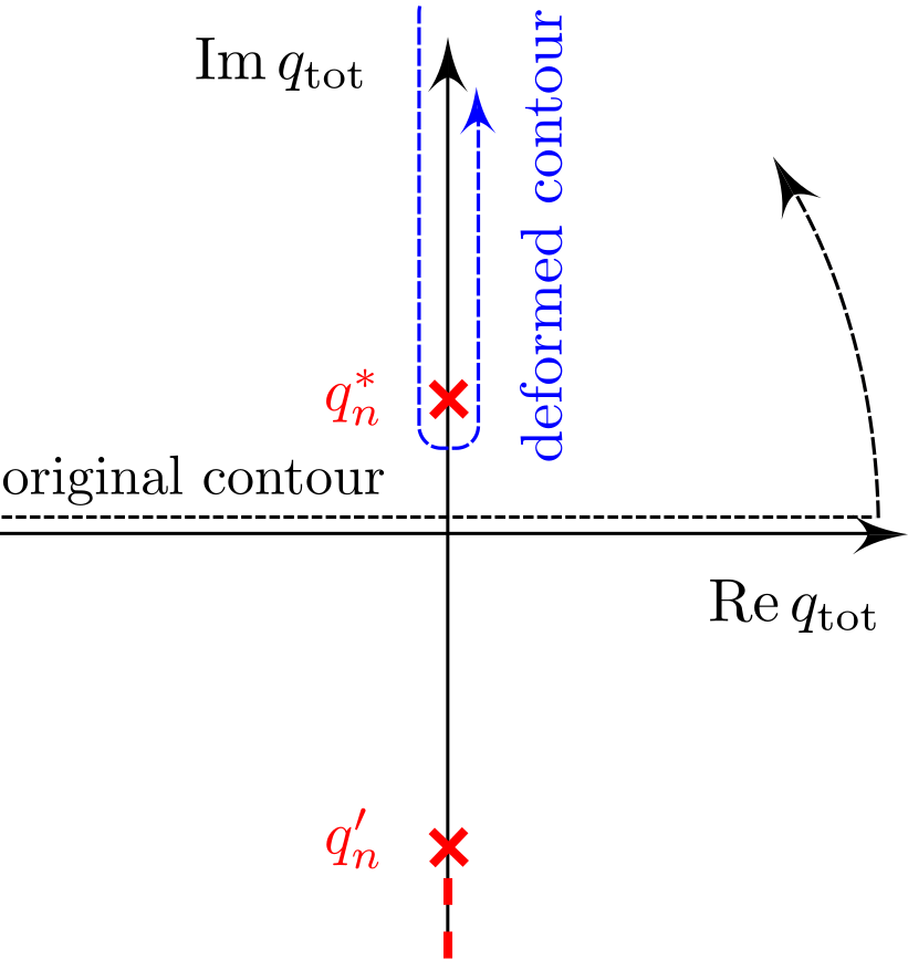
Supplementary Figure S 1: The branch-cut and contour integration in Eq. (S 23).

We thus make a crucial observation: The branch-cut in the upper complex half-plane of $q_{n}$ descends to the origin for $\alpha=0$, while the branch cut in the lower half plane always starts below $-2i\beta/\left(\beta-g_{A}\right)$. For $n>0$, the integral over the real line in the inverse Fourier transform in Eq. (S 18) can be deformed to an integral around the branch cut running from $+i\infty$ to $q_{a}^{*}$ to the left hand side of the branch cut (at a small distance $\varepsilon$, say), and then running back to infinity on the right hand side (see Fig. S 1). The half-circle around $q_{a}^{*}$ is of order $\varepsilon$ and can be neglected. We can write

$$f\left(s=0,n\right) =e^{-\frac{\alpha s_{0}}{\beta}}\int\frac{dq_{n}}{2\pi}\exp\left\{iq_{n}\left(n-s_{0}\frac{g_{A}}{\beta}\right)-s_{0}\frac{\kappa\left(q_{n}\right)}{\beta}\right\}$$

$$=e^{-\frac{\alpha s_{0}}{\beta}}\int_{\infty}^{q_{n}^{*}}\frac{idq_{n}}{2\pi}\exp\left\{-\left(q_{n}-i\varepsilon\right)\left(n-s_{0}\frac{g_{A}}{\beta}\right)-s_{0}\frac{\kappa\left(iq_{n}+\varepsilon\right)}{\beta}\right\}$$

$$\quad+e^{-\frac{\alpha s_{0}}{\beta}}\int_{q_{n}^{*}}^{\infty}\frac{idq_{n}}{2\pi}\exp\left\{-\left(q_{n}+i\varepsilon\right)\left(n-s_{0}\frac{g_{A}}{\beta}\right)-s_{0}\frac{\kappa\left(iq_{n}-\varepsilon\right)}{\beta}\right\},$$ (S 23)

On the new contour, we need

$$\kappa\left(iq_{n}\right)=\sqrt{\left(\alpha-g_{A}q_{n}\right)^{2}-\beta g_{A}q_{n}\left(q_{n}+2\right)}.$$ (S 24)

It is clear from Eq. (S 23) that the most important contribution to the integrals will come from the vicinity of $q_{n}^{*}$, because the integrand decays exponentially for larger $q_{n}$ the faster, the larger $n$. Expanding $\kappa\left(iq_{n}\right)$ around $q_{n}^{*}$, we obtain

$$\kappa\left(iq_{n}\pm\varepsilon\right)=\pm i\sqrt{2\sqrt{\beta g_{A}\left(2\alpha g_{A}+\alpha^{2}+\beta g_{A}\right)}\left(q-q_{n}^{*}\right)}$$ (S 25)

(approaching the branch cut from different sides changes the sign of the square root). Thus, for large $n$, we approximate Eq. (S 23) as

$$f\left(s=0,n\right) \approx-e^{-\frac{\alpha s_{0}}{\beta}}\int_{q_{n}^{*}}^{\infty}\frac{idq_{a}}{2\pi}\exp\left\{-q_{n}\left(n-s_{0}\frac{g_{A}}{\beta}\right)-\frac{s_{0}}{\beta}i\sqrt{2\sqrt{\beta g_{A}\left(2\alpha g_{A}+\alpha^{2}+\beta g_{A}\right)}\left(q_{n}-q_{n}^{*}\right)}\right\}$$

$$\quad+e^{-\frac{\alpha s_{0}}{\beta}}\int_{q_{n}^{*}}^{\infty}\frac{idq_{a}}{2\pi}\exp\left\{-q_{n}\left(n-s_{0}\frac{g_{A}}{\beta}\right)+\frac{s_{0}}{\beta}i\sqrt{2\sqrt{\beta g_{A}\left(2\alpha g_{A}+\alpha^{2}+\beta g_{A}\right)}\left(q_{n}-q_{n}^{*}\right)}\right\}$$

$$=-ie^{-\frac{\alpha s_{0}}{\beta}}\int_{0}^{\infty}\frac{dq_{a}}{2\pi}\exp\left\{-\left(q_{n}+q_{n}^{*}\right)\left(n-s_{0}\frac{g_{A}}{\beta}\right)-\frac{s_{0}}{\beta}i\sqrt{2pq_{n}}\right\}$$

$$\quad+ie^{-\frac{\alpha s_{0}}{\beta}}\int_{0}^{\infty}\frac{dq_{a}}{2\pi}\exp\left\{-\left(q_{n}+q_{n}^{*}\right)\left(n-s_{0}\frac{g_{A}}{\beta}\right)+\frac{s_{0}}{\beta}i\sqrt{2pq_{n}}\right\}$$

$$=2\mathrm{Im}\left(e^{-\frac{\alpha s_{0}}{\beta}}\int_{0}^{\infty}\frac{dq_{a}}{2\pi}\exp\left\{-\left(q_{n}+q_{n}^{*}\right)\left(n-s_{0}\frac{g_{A}}{\beta}\right)+\frac{s_{0}}{\beta}i\sqrt{2pq_{n}}\right\}\right)$$ (S 26)

with

$$p=\sqrt{\beta g_{A}\left(2\alpha g_{A}+\alpha^{2}+\beta g_{A}\right)}$$ (S 27)

For the remaining integral we obtain

$$f\left(s=0,n\right) \approx\frac{s_{0}\sqrt{p}e^{\frac{-ps_{0}^{2}}{2\beta^{2}\left(n-s_{0}\frac{g_{A}}{\beta}\right)}-q_{n}^{*}\left(n-s_{0}\frac{g_{A}}{\beta}\right)}}{\sqrt{2\pi}\beta\left(n-s_{0}\frac{g_{A}}{\beta}\right)^{3/2}}$$

$$\approx\frac{s_{0}\sqrt{p}e^{-q_{n}^{*}\left(n-s_{0}\frac{g_{A}}{\beta}\right)}}{\sqrt{2\pi}\beta\left(n-s_{0}\frac{g_{A}}{\beta}\right)^{3/2}}$$ (S 28)

This is a truncated, one-sided Lévy distribution (tsallis1997levy, ; gnedenko1954_stable_distr, ; bouchaud1990anomalous, ). The appearance of the Lévy distribution could have been anticipated, since the integrand of Eq. (S 18) for $\alpha=0$ can be mapped to the characteristic function of the Lévy distribution after the argument of the square root in $\kappa\left(q_{n}\right)$ has been expanded for small $q_{n}$. For small $\alpha$ and $g_{0}$ we find $g_{A}=\left(-\alpha+\beta-g_{0}\right)/2\approx\beta/2$, as well as $p\approx\beta^{2}/2$, and for $n\gg 1$ the truncated power law of Eq. (S 28) becomes Eq. (5) of the main text with $\bar{N}=1$. In the main text, we stated that the $t\rightarrow\infty$ limit of $f_{\mathrm{tot}}\left(x_{\mathrm{tot}},t\right)$ – the distribution of total lineage sizes $x_{\mathrm{tot}}$ – is governed by the same expression as $f\left(s=0,n\right)$ (see Eq. (5) of the main text). We will justify this statement below. On an intuitive level this can be understood as a consequence of the fact that, as $t$ increases, most cells will already have differentiated and $f_{\mathrm{tot}}$ will be dominated by the N-cell distribution.

Since $q_{n}^{*}$ descends to the origin as $\alpha\rightarrow 0$, the truncation of the $3/2$-power-law of (S 28) vanishes and (S 28) becomes a true Lévy stable power-law distribution. Returning to the observation that the integrand of (S 18) is nonanalytic in the lower complex half plane, we conclude that $f\left(s=0,n\right)$ is finite for $n<0$, meaning that there is a finite probability to find a negative number of N-cells. This is a consequence of approximating the discrete master equation by a continuous Fokker-Planck equation which is accurate for large $s$ and $n$. However, one can easily convince oneself that $f\left(s=0,n\right)$ decays very fast as $n$ decreases below zero: Following the reasoning of the above branch-cut integration, we see that $f\left(s=0,n\right)$ will be suppressed by an exponential factor $e^{-q_{n}^{\prime}n}$. On the other hand, we see from Eq. (S 22) that for small $\alpha$

$$\left|q_{n}^{{}^{\prime}}\right|\gg\left|q_{n}^{*}\right|$$ (S 29)

holds. Thus we conclude that the probability for a negative $n$ is very small, and can be neglected as an artifact of the Fokker-planck approximation. Notice that the probability for negative $s$ is zero, because Eq. (S 12) is analytic in $q_{s}$, except for a single pole which is always in the upper complex half plane (since $\mathrm{Re}\left(\lambda\left(q_{n}\right)>0\right)$ as Eqs. (S 14), (S 13) indicate). Indeed, while the diffusion coefficient associated with the second derivative in $s$ in Eq. (3) vanishes at $s=0$, the diffusion coefficient associated with $n$-diffusion does not vanish at the origin and allows for a small leakage of probability towards negative $n$.

So far we have been investigating the analytic structure of the $s=0$ contribution to $\tilde{f}\left(\mathbf{q},t\right)$. However similar arguments carry over to the general case. Multiplying the numerator and denominator of the function $G\left(q_{s},q_{n},t\right)$ in Eq. (S 13) by $\lambda\left(q_{n},t\right)^{-1}$ and keeping $q_{s}$ real for the moment, we see, that the characteristic function $\tilde{f}\left(\mathbf{q},t\right)$ (Eq. (S 12)) is analytic in $q_{n}$ except for the branch-cuts of $\kappa\left(q_{n}\right)$ and the pole at $\lambda\left(q_{n},t\right)=i/q_{s}$. This pole occurs when $\lambda\left(q_{n},t\right)$ is purely imaginary. $f\left(s,n,t\right)$ will decay for $n<0$ the faster, the lower the nonanalyticities with $\mathrm{Im}\left(q_{n}\right)<0$ lie in the complex plane. Eq. (S 29) shows that the contribution of the lower half branch-cut is indeed negligible since it starts much further away from the origin than the upper branch-cut. A numerical inspection of $\lambda\left(q_{n},t\right)$ shows that regions where $\lambda\left(q_{n},t\right)$ is purely imaginary in the lower complex half plane of $q_{n}$ are indeed sufficiently far from the origin for all reasonable parameter choices. We conclude that the finite values of $f\left(s,n,t\right)$ for negative $n$ are simply an artifact of the Fokker-Planck approximation to the original master equation (1) and are small.

Supplementary Sec..1.3 The lineage size distribution $f_{\mathrm{tot}}\left(x_{\mathrm{tot}},t\right)$

As pointed out in the main text, we are ultimately interested in the distribution of the lineage size

$$x_{\mathrm{tot}}=s+n.$$ (S 30)

This distribution is obtained by summing $f\left(s,n,t\right)$ over all states which satisfy the condition (S 30):

$$f_{\mathrm{tot}}\left(x_{\mathrm{tot}},t\right)=\int_{0}^{x_{\mathrm{tot}}}f\left(s,x_{\mathrm{tot}}-s,t\right)ds$$ (S 31)

(see also Eq. (4) in the main text). Having argued in Sec. Supplementary Sec..1.2, that the distribution $f\left(s,n,t\right)$ corresponding to the characteristic function (S 12) is confined to positive $s$ and – to a good approximation – to positive $n$, we can extend the integration in Eq. (S 31) to the complete real axis:

$$f\left(x_{\mathrm{tot}},t\right)\approx\int_{-\infty}^{\mathrm{\infty}}ds\,f\left(s,x_{\mathrm{tot}}-s,t\right).$$

A Fourier transform then gives

$$\tilde{f}\left(q_{\mathrm{tot}},t\right)\approx\tilde{f}\left(q_{s}=q_{\mathrm{tot}},q_{n}=q_{\mathrm{tot}},t\right),$$ (S 32)

where the characteristic function of Eq. (S 12) is on the right hand side. This yields

$$\tilde{f}\left(q_{\mathrm{tot}},t\right)=\exp\left(\frac{q_{\mathrm{tot}}s_{0}\left[\alpha+2g_{A}+\kappa\left(q_{\mathrm{tot}}\right)\coth\left(\frac{1}{2}\kappa\left(q_{\mathrm{tot}}\right)t\right)\right]}{-i\alpha+g_{A}q_{\mathrm{tot}}-\beta q_{\mathrm{tot}}+i\kappa\left(q_{\mathrm{tot}}\right)\coth\left(\frac{1}{2}\kappa\left(q_{\mathrm{tot}}\right)t\right)}\right).$$ (S 33)

Analytic expressions for the power-law and avalanche regimes

The characteristic function given in Eq. (S 33) has a peculiar behavior at $q_{\mathrm{tot}}=0$ which determines the asymptotics for large $x_{\mathrm{tot}}$. To see this, let us first investigate the $t\rightarrow\infty$ and the $q_{\mathrm{tot}}\rightarrow\infty$ limits of $\tilde{f}\left(q_{\mathrm{tot}},t\right)$. Since $\mathrm{Re}\kappa\left(q_{\mathrm{tot}}\right)>0$ holds for all real $q_{\mathrm{tot}}$ (see Eq. (S 14)) and $\mathrm{Re}\kappa\left(q_{\mathrm{tot}}\right)\sim\left|q_{\mathrm{tot}}\right|$ for large arguments, the approximation

$$\coth\left(\frac{1}{2}\kappa\left(q_{\mathrm{tot}}\right)t\right)\sim 1+2e^{-\kappa\left(q_{\mathrm{tot}}\right)t}$$ (S 34)

holds in both, the $t\rightarrow\infty$ and the $q_{\mathrm{tot}}\rightarrow\infty$ limits. Using (S 34), Eq. (S 33) can be approximated by

$$\tilde{f}\left(q_{\mathrm{tot}}\rightarrow\infty,t\right)\approx\tilde{f}\left(q_{\mathrm{tot}},t\rightarrow\infty\right)\approx\exp\left(-s_{0}\frac{ig_{A}q_{\mathrm{tot}}+\alpha+\kappa\left(q_{\mathrm{tot}}\right)}{\beta}\right).$$ (S 35)

For $\alpha>0$, this expression approaches $\exp\left(-2\alpha s_{0}/\beta\right)$ as $q_{\mathrm{tot}}\rightarrow 0$, whereas for $\alpha\leq 0$, it approaches unity. For the full characteristic function, however, $\tilde{f}\left(q_{\mathrm{tot}},t\right)=1$ is true in all cases. This is depicted in Fig. S 2. We conclude that Eq. (S 35) is not a good approximation for small $\left|q_{\mathrm{tot}}\right|$ if $\alpha>0$ holds. To find an approximation for small $\left|q_{\mathrm{tot}}\right|$ and positive growth rates, we expand the numerator and denominator inside the exponential function in Eq. (S 33) around $q_{\mathrm{tot}}\approx 0$ and find

$$q_{\mathrm{tot}}s_{0}\left[\alpha+2g_{A}+\kappa\left(q_{\mathrm{tot}}\right)\coth\left(\frac{1}{2}\kappa\left(q_{\mathrm{tot}}\right)t\right)\right]\approx q_{\mathrm{tot}}s_{0}\left[\alpha+2g_{A}+\left|\alpha\right|\coth\left(\frac{\left|\alpha\right|t}{2}\right)\right]$$

and

$$-i\alpha+g_{A}q_{\mathrm{tot}}-\beta q_{\mathrm{tot}}+i\kappa\left(q_{\mathrm{tot}}\right)\coth\left(\frac{1}{2}\kappa\left(q_{\mathrm{tot}}\right)t\right) \approx i\left(\left|\alpha\right|\coth\left(\frac{\left|\alpha\right|t}{2}\right)-\alpha\right)+\frac{q_{\mathrm{tot}}\Xi\left(t\right)}{2\left|\alpha\right|},$$

where

$$\Xi\left(t\right) =\text{csch}^{2}\left(\frac{\left|\alpha\right|t}{2}\right)\left[\left|\alpha\right|\left(\beta+g_{A}\left(t\left(\alpha+\beta\right)-1\right)\right)-g_{A}\left(\alpha+\beta\right)\sinh\left(\left|\alpha\right|t\right)+\left|\alpha\right|\left(g_{A}-\beta\right)\cosh\left(\left|\alpha\right|t\right)\right]$$

$$\approx-\beta^{2}\coth\left(\frac{\left|\alpha\right|t}{2}\right)$$

In the last line we assumed that $\left|\alpha\right|\ll\beta$. Therefore, the appropriate approximation for $\alpha>0$ and small $\left|q_{\mathrm{tot}}\right|$ reads

$$\tilde{f}\left(q_{\mathrm{tot}}\rightarrow 0,t\right)\approx\exp\left(\frac{q_{\mathrm{tot}}s_{0}\left[\alpha+2g_{A}+\left|\alpha\right|\coth\left(\frac{\left|\alpha\right|t}{2}\right)\right]}{i\left(\left|\alpha\right|\coth\left(\frac{\left|\alpha\right|t}{2}\right)-\alpha\right)+\frac{q_{\mathrm{tot}}\Xi\left(t\right)}{2\left|\alpha\right|}}\right).$$ (S 36)

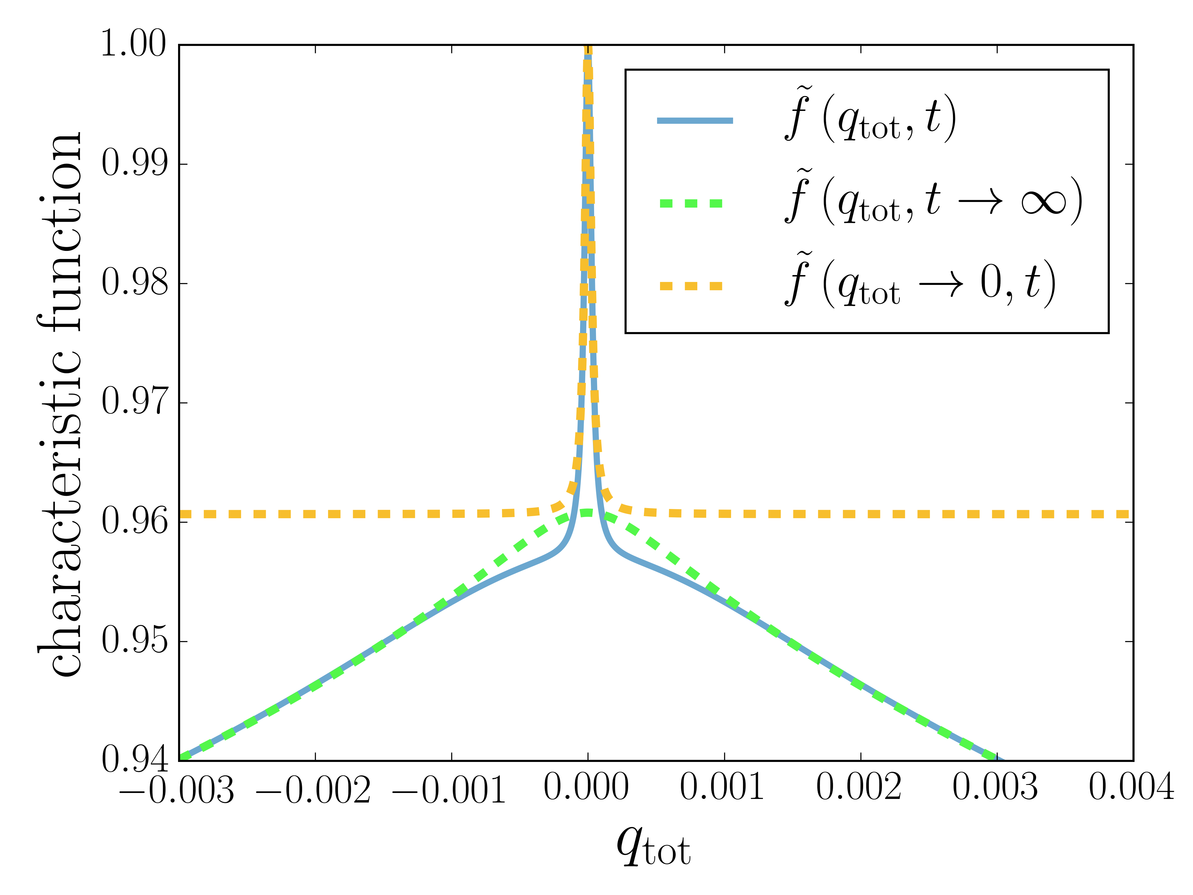
Supplementary Figure S 2: The full characteristic function $\tilde{f}\left(q_{\mathrm{tot}},t\right)$ of Eq. (S 33) and the approximations for $t\rightarrow\infty$ or large $q_{\mathrm{tot}}$, $\tilde{f}\left(q_{\mathrm{tot}},t\rightarrow\infty\right)$, (Eq. (S 35)), as well as for small $q_{\mathrm{tot}}$, $\tilde{f}\left(q_{\mathrm{tot}}\rightarrow 0,t\right)$, (Eq.S 36). We used a positive growth rate $\alpha=0.2/\mathrm{day}$ and $\beta=10/\mathrm{day}$. For $\alpha>0$ and large but finite $t$, $\tilde{f}\left(q_{\mathrm{tot}},t\rightarrow\infty\right)$ (green dashed curve) is a good approximation to the characteristic function $\tilde{f}\left(q_{\mathrm{tot}},t\right)$ (blue curve), except for a small region near $q_{\mathrm{tot}}=0$ which is well approximated by $\tilde{f}\left(q_{\mathrm{tot}}\rightarrow 0,t\right)$ (orange curve). This region governs the behavior at large lineage sizes $x_{\mathrm{tot}}$.

It remains to determine the distribution function $f\left(x_{\mathrm{tot}},t\right)$. At small and intermediate $x_{\mathrm{tot}}$, we expect $f\left(x_{\mathrm{tot}},t\right)$ to be governed by the behavior of the characteristic function at larger $q_{\mathrm{tot}}$, whereas the behavior of $f\left(x_{\mathrm{tot}},t\right)$ for large $x_{\mathrm{tot}}$ will be determined by the region around $q_{\mathrm{tot}}\approx 0$. This has to do with the analytic structure of Eq. (S 33). The question is, which nonanalyticity dominates the Fourier transform as the integration contour is deformed according to Fig. S 1. Besides the branch-cuts of $\kappa\left(q_{n}\right)$, $\tilde{f}\left(q_{\mathrm{tot}},t\right)$ exhibits a pole on the imaginary axis (see Fig. S 3). Let this pole be located at $q_{\mathrm{tot}}=iq_{\mathrm{tot}}^{*}$. If it is closer to the origin than the upper starting point of the branch-cut, i.e. $q_{\mathrm{tot}}^{*}<q_{n}^{*}$, where $q_{n}^{*}$ is defined in Eq. (S 19), the pole becomes dominant at large $x_{\mathrm{tot}}$. This is because both nonanalyticities, the branch cut starting at $q_{n}^{*}$ and the pole at $q_{\mathrm{tot}}^{*}$, are located on the positive imaginary axis. Hence, when the integration along the deformed contour is performed, the contributions of the pole and the branch-cut will roughly behave as $e^{-q_{\mathrm{tot}}^{*}x_{\mathrm{tot}}}$, or $e^{-q_{n}^{*}x_{\mathrm{tot}}}$, respectively. We can use Eq. (S 36) to track the behavior of $q_{\mathrm{tot}}^{*}$ for different parameter values:

$$iq_{\mathrm{tot}}^{*} =\frac{-2i\left|\alpha\right|}{\Xi\left(t\right)}\left(\left|\alpha\right|\coth\left(\frac{\left|\alpha\right|t}{2}\right)-\alpha\right)\approx 2i\frac{\alpha^{2}}{\beta^{2}}\left(1-\mathrm{sign}\left(\alpha\right)\tanh\left(\frac{\left|\alpha\right|t}{2}\right)\right).$$ (S 37)

Eq. (S 37) shows that the analytic structure of the characteristic function is very different for positive and negative $\alpha$. For positive $\alpha$, it is $q_{\mathrm{tot}}^{*}<q_{n}^{*}$, and therefore $f\left(x_{\mathrm{tot}},t\right)$ will be dominated by the single pole that is captured in Eq. (S 37). For $\alpha<0$, the opposite scenario is true: we find $q_{n}^{*}<q_{\mathrm{tot}}^{*}$.

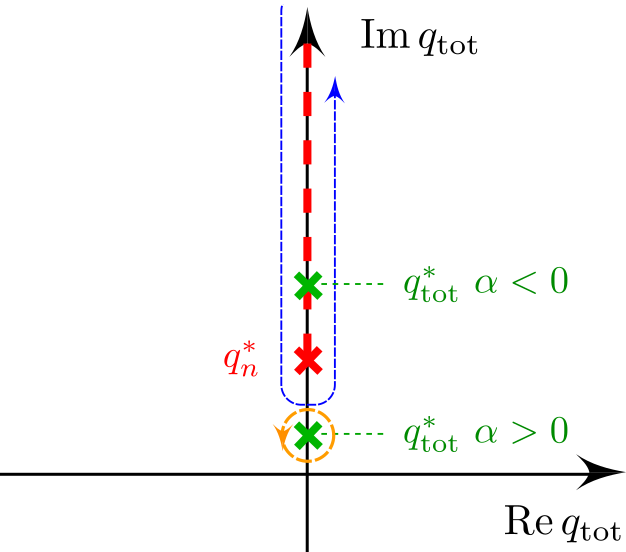
Supplementary Figure S 3: Branch-cut integration (see Fig. S 1 and Eq. (S 23)) and the pole at $q_{\mathrm{tot}}^{*}$ (Eq. (S 37)) characterizing the avalanche part of the distribution. Both, the pole and the branch-cut must be captured by the deformed contour (blue dashed line). For $\alpha>0$, the pole at $q_{\mathrm{tot}}^{*}$ is always nearer to the origin than the starting point of the branch-cut $q_{n}^{*}$ and thus determines the large $x_{\mathrm{tot}}$ behavior. For $\alpha<0$, $q_{\mathrm{tot}}^{*}$ is within the integration contour, moving towards larger imaginary values as $t$ is increased. For sufficiently small $t$, the avanlanche part of the distribution is still well approximated by the integration around the $q_{\mathrm{tot}}^{*}$ pole (see Fig. 2 b)).

We now calculate the inverse Fourier transforms Eqs. (S 35) and (S 36) which will give us approximate expressions for $f\left(x_{\mathrm{tot}},t\right)$ at intermediate and large $x_{\mathrm{tot}}$. The inverse Fourier transform of Eq. (S 35) reads

$$f_{\mathrm{tot}}^{t\rightarrow\infty}\left(x_{\mathrm{tot}}\right)\equiv\int\frac{dq_{\mathrm{tot}}}{2\pi}e^{iq_{\mathrm{tot}}x_{\mathrm{tot}}}\lim_{t\rightarrow\infty}\tilde{f}\left(q_{\mathrm{tot}},t\right)=e^{-\frac{\alpha}{\beta}s_{0}}\int\frac{dq_{n}}{2\pi}\exp\left(iq_{\mathrm{tot}}\left(x_{\mathrm{tot}}-s_{0}\frac{g_{A}}{\beta}\right)-s_{0}\frac{\kappa\left(q_{\mathrm{tot}}\right)}{\beta}\right).$$ (S 38)

We encountered this integral when we calculated the distribution of N-cells in Eq. (S 18). Similarly to Eq. (S 28) we find

$$f_{\mathrm{tot}}^{t\rightarrow\infty}\left(x_{\mathrm{tot}}\right)=\frac{s_{0}\sqrt{p}e^{\frac{-ps_{0}^{2}}{2\beta^{2}\left(x_{\mathrm{tot}}-s_{0}\frac{g_{A}}{\beta}\right)}-q_{\mathrm{tot}}^{*}\left(x_{\mathrm{tot}}-s_{0}\frac{g_{A}}{\beta}\right)}}{\sqrt{2\pi}\beta\left(x_{\mathrm{tot}}-s_{0}\frac{g_{A}}{\beta}\right)^{3/2}}$$ (S 39)

with

$$p =\sqrt{\beta g_{A}\left(2\alpha g_{A}+\alpha^{2}+\beta g_{A}\right)}$$

$$q_{n}^{*} =\frac{\alpha^{2}}{g_{A}\left(\alpha+\beta\right)+\sqrt{\beta g_{A}\left(\alpha^{2}+2\alpha g_{A}+\beta g_{A}\right)}}.$$

In order to account for the $\bar{N}$ N-cells that each S-cell is producing we have to make the substitution $q_{\mathrm{n}}\rightarrow\bar{N}q_{n}$ in Eq. (S 32). This substitution carries over to Eq. (S 35) where we have to replace $q_{\mathrm{tot}}$ by $\bar{N}q_{\mathrm{tot}}$. The integration of Eq. (S 38) is evaluated according to

$$\int\frac{dq_{\mathrm{tot}}}{2\pi}e^{iq_{\mathrm{tot}}x_{\mathrm{tot}}}\lim_{t\rightarrow\infty}\tilde{f}\left(\bar{N}q_{\mathrm{tot}},t\right)=\int\frac{dq^{\prime}_{\mathrm{tot}}}{\bar{N}2\pi}e^{iq^{\prime}_{\mathrm{tot}}x_{\mathrm{tot}}/\bar{N}}\lim_{t\rightarrow\infty}\tilde{f}\left(q^{\prime}_{\mathrm{tot}},t\right)=\frac{1}{\bar{N}}f_{\mathrm{tot}}^{t\rightarrow\infty}\left(x_{\mathrm{tot}}/\bar{N}\right).$$ (S 40)

For $\left|\alpha\right|\ll\beta$, we obtain the result of Eq. (5), Sec. Regimes of growth: power-laws and avalanches of the main text:

$$f_{\mathrm{tot}}^{t\rightarrow\infty}\left(x_{\mathrm{tot}}\right)\approx\frac{s_{0}\beta e^{-\frac{\alpha^{2}x_{\mathrm{tot}}}{\beta^{2}\bar{N}}}}{2\sqrt{2\pi}\bar{N}\left(x_{\mathrm{tot}}/\bar{N}\right)^{3/2}}.$$ (S 41)

According to the above discussion, Eq. (S 41) is valid for intermediate $x_{\mathrm{tot}}$ if $\alpha>0$. For$\alpha<0$, the contribution of the pole becomes stronger and stronger sub-leading to the branch-cut contribution as $t$ is increased (see Eq. (S 37)). However, if $t$ is sufficiently small, the pole is in the vicinity of the branch-cut starting point $q_{n}^{*}$ and has a strong influence on the distribution function. For large enough $t$ however, Eq. (S 41) is a good approximation for $f_{\mathrm{tot}}\left(x_{\mathrm{tot}}\right)$ everywhere.

To determine the behavior at large $x_{\mathrm{tot}}$ for $\alpha>0$ we make use of Eq. (S 36) which gives a good approximation for the characteristic function at small $q_{\mathrm{tot}}$. It is useful to rewrite Eq. (S 41) as

$$\tilde{f}\left(q_{\mathrm{tot}}\rightarrow 0,t\right)=e^{-aq_{\mathrm{tot}}^{*}}\exp\left(\frac{aq_{\mathrm{tot}}^{*}}{1+iq_{\mathrm{tot}}/q_{\mathrm{tot}}^{*}}\right)$$

with

$$a=\frac{s_{0}\left(\alpha+2g_{A}+\alpha\coth\left(\frac{\alpha t}{2}\right)\right)}{\alpha\left(\coth\left(\frac{\alpha t}{2}\right)-1\right)}.$$ (S 42)

The inverse Fourier transform

$$f_{\mathrm{tot}}\left(x_{\mathrm{tot}}\rightarrow\infty,t\right)=e^{-aq_{\mathrm{tot}}^{*}}\int\frac{dq_{\mathrm{tot}}}{2\pi}\exp\left(iq_{\mathrm{tot}}x_{\mathrm{tot}}+\frac{aq_{\mathrm{tot}}^{*}}{1+iq_{\mathrm{tot}}/q_{\mathrm{tot}}^{*}}\right)$$ (S 43)

is strictly speaking divergent (as is the one in Eq. (S 17)). However it can be regularized by adding a small exponential factor $e^{-q_{\mathrm{tot}}\left|\varepsilon\right|}$ to the integrand and letting $\varepsilon\rightarrow 0$ after the integral is done. The large $x_{\mathrm{tot}}$ behavior that we are interested in is dominated by the pole at $q_{\mathrm{tot}}^{*}$ for $\alpha>0$. We will see later, that for $\alpha<0$, the pole still dominates the distribution for reasonably large $x_{\mathrm{tot}}$ (avalanche regime) if $t$ is small, although it does not govern the asymptotics for $x_{\mathrm{tot}}\rightarrow\infty$ . The pole’s contribution can be found by integrating along a circle around $q_{\mathrm{tot}}^{*}$ (see Fig. S 3). Writing

$$q_{\mathrm{tot}}=iq_{\mathrm{tot}}+re^{i\varphi}$$

the integral around the pole at $q_{\mathrm{tot}}$ becomes

$$f_{\mathrm{tot}}\left(x_{\mathrm{tot}}\rightarrow\infty,t\right) =\exp\left(-\frac{a}{q_{\mathrm{tot}}}-\frac{x_{\mathrm{tot}}}{q_{\mathrm{tot}}}\right)ir\int_{0}^{2\pi}\frac{e^{i\varphi}d\varphi}{2\pi}\exp\left(ire^{i\varphi}x_{\mathrm{tot}}+\frac{a}{iq_{\mathrm{tot}}^{2}re^{i\varphi}}\right).$$

Since the radius $r$ is arbitrary, we are free to chose

$$r=\sqrt{\frac{a}{q_{\mathrm{tot}}^{2}x_{\mathrm{tot}}}}.$$

After some algebra, we arrive at

$$f_{\mathrm{tot}}\left(x_{\mathrm{tot}}\rightarrow\infty,t\right)=\exp\left(-\frac{a}{q_{\mathrm{tot}}}-\frac{x_{\mathrm{tot}}}{q_{\mathrm{tot}}}\right)r\int_{0}^{2\pi}\frac{e^{i\varphi}d\varphi}{2\pi}\exp\left(rx_{\mathrm{tot}}\left[e^{i\varphi}+\frac{1}{e^{i\varphi}}\right]\right).$$ (S 44)

Using the integral representation of Bessel functions

$$I_{n}\left(z\right)=\frac{1}{2\pi i}\int_{\mathcal{C}}dt\frac{e^{\frac{z}{2}\left(t+\frac{1}{t}\right)}}{t^{n+1}},$$

where $\mathcal{C}$ is a contour enclosing the origin, with the substitution $t=e^{i\varphi}$ Eq. (S 44) becomes

$$f_{\mathrm{tot}}\left(x_{\mathrm{tot}}\rightarrow\infty,t\right)=\theta\left(x_{s}\right)\exp\left(-\frac{a}{q_{\mathrm{tot}}}-\frac{x_{\mathrm{tot}}}{q_{\mathrm{tot}}}\right)\sqrt{\frac{a}{q_{\mathrm{tot}}^{2}x_{\mathrm{tot}}}}I_{1}\left(2\sqrt{\frac{ax_{\mathrm{tot}}}{q_{\mathrm{tot}}^{2}}}\right).$$ (S 45)

For $\alpha>0$, this is the large $x_{\mathrm{tot}}$ approximation for the distribution function $f\left(x_{\mathrm{tot}},t\right)$ given in Eq. (6), where we have restored the variable $\bar{N}$. As is demonstrated in Fig. (2), Eq. (S 45) provides a good approximation for the large $x_{\mathrm{tot}}$ behavior of $f_{\mathrm{tot}}\left(x_{\mathrm{tot}},t\right)$ for a positive S-cell growth rate $\alpha$. However, even for $\alpha<0$, at reasonably large $x_{\mathrm{tot}}$ (namely in the avalanche regime), the behavior of the lineage size probability density is well described by Eq. (S 45), if $\alpha t\lesssim 1$ holds. This is due to the fact that the pole at $q_{\mathrm{tot}}^{*}$, while located above $q_{n}^{*}$ on the imaginary $q_{\mathrm{tot}}$ line (see Fig. S 3), is still sufficiently near $q_{n}^{*}$to dominate the avalanche part of the distribution function (see Eq. (S 37)). However, the asymptotics of $f_{\mathrm{tot}}\left(x_{\mathrm{tot}},t\right)$ for $x_{\mathrm{tot}}\rightarrow\infty$ will not be given by Eq. (S 45). Since in both cases, for positive and negative $\alpha$, Eq. (S 45) is an approximation for the avalanche part of the lineage size probability density, we call it $f_{\mathrm{tot}}^{\mathrm{av.}}\left(x_{\mathrm{tot}},t\right)$.

Supplementary Sec..2 Most-likely paths

We now derive the most likely path $s_{\tau}(t)$ that a critical S-cell population (i.e. $\alpha=0$) takes from $s_{0}$ cells at $t=0$ to extinction at $t=\tau$. Since we consider only S-cells and only critical populations, equation (3), accorting to the rules of Ito’s calculus, reduces a process described by the stochastic differential equation (SDE)

$$ds=\sqrt{{\beta s}}dw(t)$$ (S 46)

where $w(t)$ is the standard Brownian motion. If the set of possible paths was finite-dimensional, we could proceed by finding the density $W$ defined by equation (S 46) on the set of possible paths starting at $s_{0}$ and maximizing $W(s_{\tau})$ subject to $s_{\tau}(\tau)=0$ to find $s_{\tau}$. It turns out, however, that this approach only cleanly generalizes to infinite-dimensional path spaces in the case of a constant diffusion term (durr_onsager-machlup_1978, ). To avoid these technical difficulties, we perform a change of variable to transform equation (S 46) into a process with a constant diffusion term. By setting $y(t)=2\sqrt{s\left(t\right)/\beta}$ and applying Itô’s lemma we get

$$dy=A(y)dt+dw(t)\text{{\ where\ }A(y)=$-\frac{{1}}{2y}$}$$ (S 47)

(were once $y$ reaches zero, we define it to remain there, despite $A$ becoming undefined). For this process, the density functional $W$ expressed in terms of its Lagrangian $L$ (also called Onsager-Machlup function) is (durr_onsager-machlup_1978, )

$$W[y(t)] \sim e^{-S(y)}$$ (S 48)

$$\text{{where\ }}S\left[y\right] = \frac{{1}}{2}\int_{0}^{T}L(y,\dot{y})dt$$

$$\text{{and\ }}L(y,\dot{y}) = (\dot{y}-A(y))^{2}+A^{\prime}(y).$$

The functional $W$ defines a probability density on the set of paths in the following sense: The probability for a random path to lie within a small tube of diameter $\epsilon$ around a given differentiable path $y$ is asymptotically proportional to $W[y]H(\epsilon)$ for some function $H$ independent of $y$ (this factorization fails if the diffusion term is not constant (durr_onsager-machlup_1978, )). We can therefore proceed as we would in the finite-dimensional case and maximize $W$ to find $y_{\tau}$. Since maximizing $W$ means minimizing the action $S(y)=\frac{{1}}{2}\int_{0}^{T}L(y,\dot{y)dt}$, the desired $y_{\tau}$ is found by solving the Euler-Lagrange (EL) equation $\frac{{d}}{dt}\frac{{\partial L}}{\partial\dot{y}}=\frac{{\partial L}}{\partial y}$. In our case the EL equation yields $\ddot{y}=-\frac{{3}}{4}y^{-3}$ with the general solution

$$y(t) = \sqrt{{\lambda t^{2}+\text{$\mu t$+$\nu$}}}$$ (S 49)

$$\textrm{{where\ }}\mu^{2} = 4\lambda\nu+3,$$

and solving for the boundary conditions $y(0)=u(s_{0})=2\sqrt{{s_{0}/\beta}}$ and $y(\tau)=0$ yields

$$\nu= s_{0}\frac{{4}}{\beta}, \mu=\sqrt{{3}}-2\frac{{\nu}}{\tau}, \lambda=\frac{{1}}{\tau}\left(\frac{{\nu}}{\tau}-\sqrt{3}\right)$$

(where we chose the solution that ensures $\lambda t^{2}+\text{$\mu t$+$\nu$}>=0$ on $[0,\tau]$). Inserting these parameters into the general solution (S 49) and transforming back from $y$ to $s$ produces after some rearrangements the extinction trajectory stated in equation (9).

Supplementary Sec..3 Full Fokker-Planck equation and the simplification of the A$\rightarrow$A+N process

The full Fokker-Planck equation for the SAN process of Fig 1 of the main text is given by

$$\frac{\partial f\left(\mathbf{x},t\right)}{\partial t} = -\alpha\frac{\partial}{\partial s}sf\left(\mathbf{x},t\right)+\frac{\beta}{2}\frac{\partial^{2}}{\partial s^{2}}sf\left(\mathbf{x},t\right)$$ (S 50)

$$-\frac{\partial}{\partial a}g_{A}sf\left(\mathbf{x},t\right)+\frac{1}{2}\frac{\partial^{2}}{\partial a^{2}}g_{A}sf\left(\mathbf{x},t\right)-g_{A}\frac{\partial}{\partial s}\frac{\partial}{\partial a}x_{s}f\left(\mathbf{x},t\right).$$

$$-g_{N}\frac{\partial}{\partial n}af\left(\mathbf{x},t\right)+\frac{g_{N}}{2}\frac{\partial^{2}}{\partial n^{2}}af\left(\mathbf{x},t\right),$$

where $\mathbf{x}=\left(s,a,n\right)$ is the vector of S, A, and N-cell counts. The simplification of the A$\rightarrow$A+N process used in our calculations is that each A-cell, on average, produces $\bar{N}$ N-cells. This, essentially, amounts to cutting the last line of the above equation and rescaling the the $a$ variable by a factor of $\bar{N}$, giving Eq. (2) of the main text.

Our justification for this simplification is that, while fluctuations in the number of S-cells $s$ scale as $\sim\sqrt{s}$ (see also Eq. (S 46)), the fluctuations of the N-cell count are - for a given $a$ - Gaussian. This can be estimated from the diffusion term in the last line. While the large $\sim\sqrt{s}$ fluctuations of the stem-cell number ultimately lead to the power-law at criticality, the Gaussian fluctuations of the number of neurons lead only to a broadening of the distributions. Llorca et. al. - eLife, 2019 (see main text for the full reference) considered the neuronal output of precurser cells (radial glia cells, which correspond to our A cells), and found that its uncertainty is only about an order of magnitude in size. As this is uncertainty is small compared to the uncertainty of the power-law distribution of total cell counts, we choose the simplified model, which is analytically tractable.

Supplementary Sec..4 Kolmogorov-Smirnov tests of the lineage size distribution

To ascertain our results, we performed Kolmogorov-Smirnov tests of the empirical data and our theoretical results for the pdf at day 40. Since our conclusion that the growth process is close to criticality is true for any parameter values within the given error margins of our fits (Table 1), but the K-S statistic is expected to strongly depend on which values are chosen ( as is obvious from a visual evaluation of the error margins of Fig. 2), we believe that what should be tested, is the distribution for intermediate lineage sizes (say between $\sim 200$ and $\sim 2000$). Here, the distribution is both close to a 3/2 power-law and mostly independent on the dynamical parameters of the model. As expected, the precise p-values of the K-S test strongly depend on the interval under consideration, but they support, in general, the SAN-model hypothesis ($p>0.1$). The highest p-values are obtained for lineage sizes between 450 and 1500. Here, the p-value is $p=0.81$, with the data comprising 1402 lineages.

The following plot shows the p-values of all intervals between $x_{\mathrm{tot}}=100$ and $x_{\mathrm{tot}}=4000$. As expected, we find a cluster of significant p values between $x_{\mathrm{tot}}\approx 200$ and $x_{\mathrm{tot}}\approx 2000$, corresponding to the region where the power-law is most pronounced. Surprisingly, there is also a cluster of high p-values between $x_{\mathrm{tot}}\approx 2000$ and $x_{\mathrm{tot}}\approx 3500$ (this region is comprised of $\sim 400$ data points) – corresponding to the region containing the avalanche of active s-cells and the exponential truncation at large $x_{\mathrm{tot}}$. In contrast, the data in the crossover between the power-law region and the truncation region does not produce high p values. We assume, that the uncertainties and systematic errors of our model have more weight in this region of the distribution.

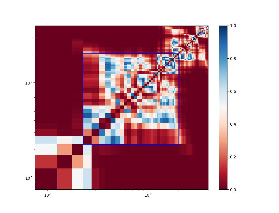
Supplementary Figure S 4: $p$-values of the Kolmogorov-Smirnov test comparing the theoretical probability distribution of the SAN model to the data at day 40 on different intervals along the axis of total cell counts $x_{\mathrm{tot}}$. The figure should be read as follows: choose an interval between $x_{\mathrm{tot,min}}$ and $x_{\mathrm{tot,max}}$ in which the data should be compared to the theoretical distribution. The color map at the point $x=x_{\mathrm{tot,min}}$ and $y=x_{\mathrm{tot,max}}$ (or the other way around) gives the $p$-value on the given interval. Intervals between 225 and 2000 - the cell counts for which the power-law is most pronounced - lie within the blue rectangle.

Supplementary Sec..5 Histograms of the data for different bin sizes

In the following the show a comparison between the probability density functions of the SAN model and histograms of the total cell count data for different bin sizes. We find that the agreement is largely independent of the bin size. The plots correspond to Fig 2 a) of the main text, with altered bin sizes for the data.

      

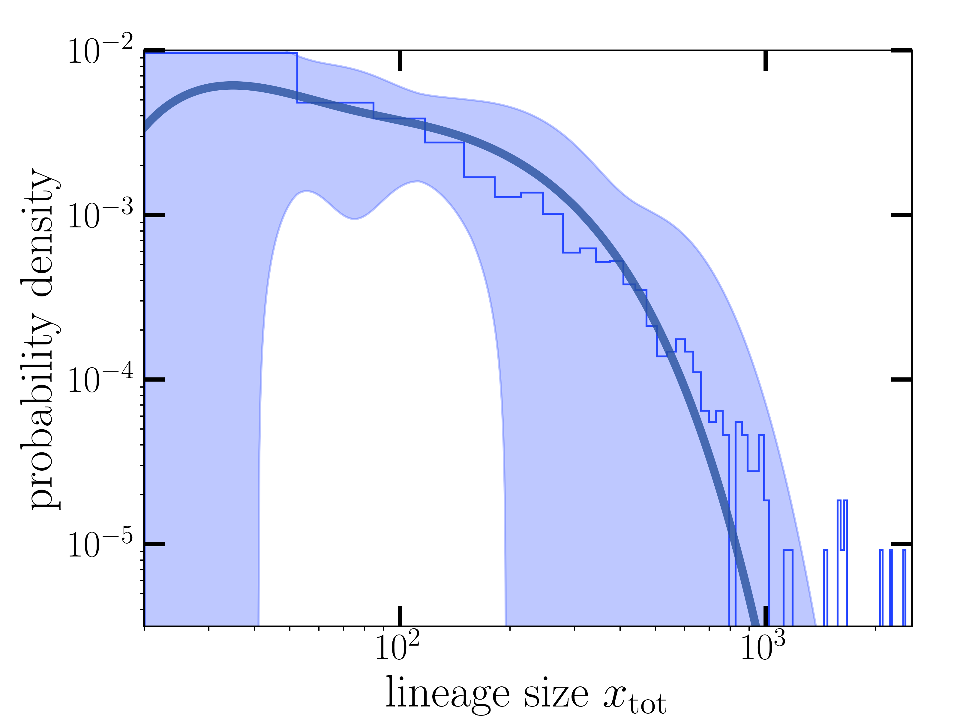
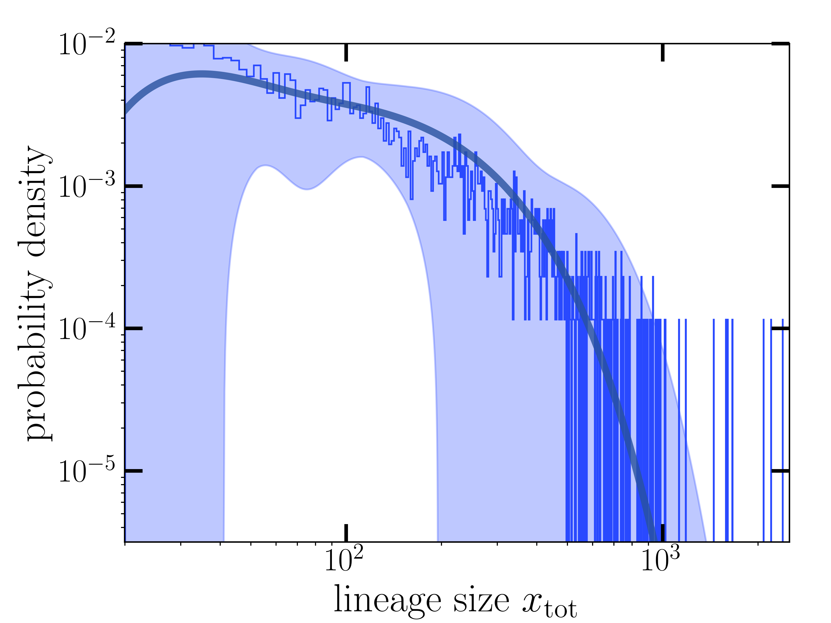
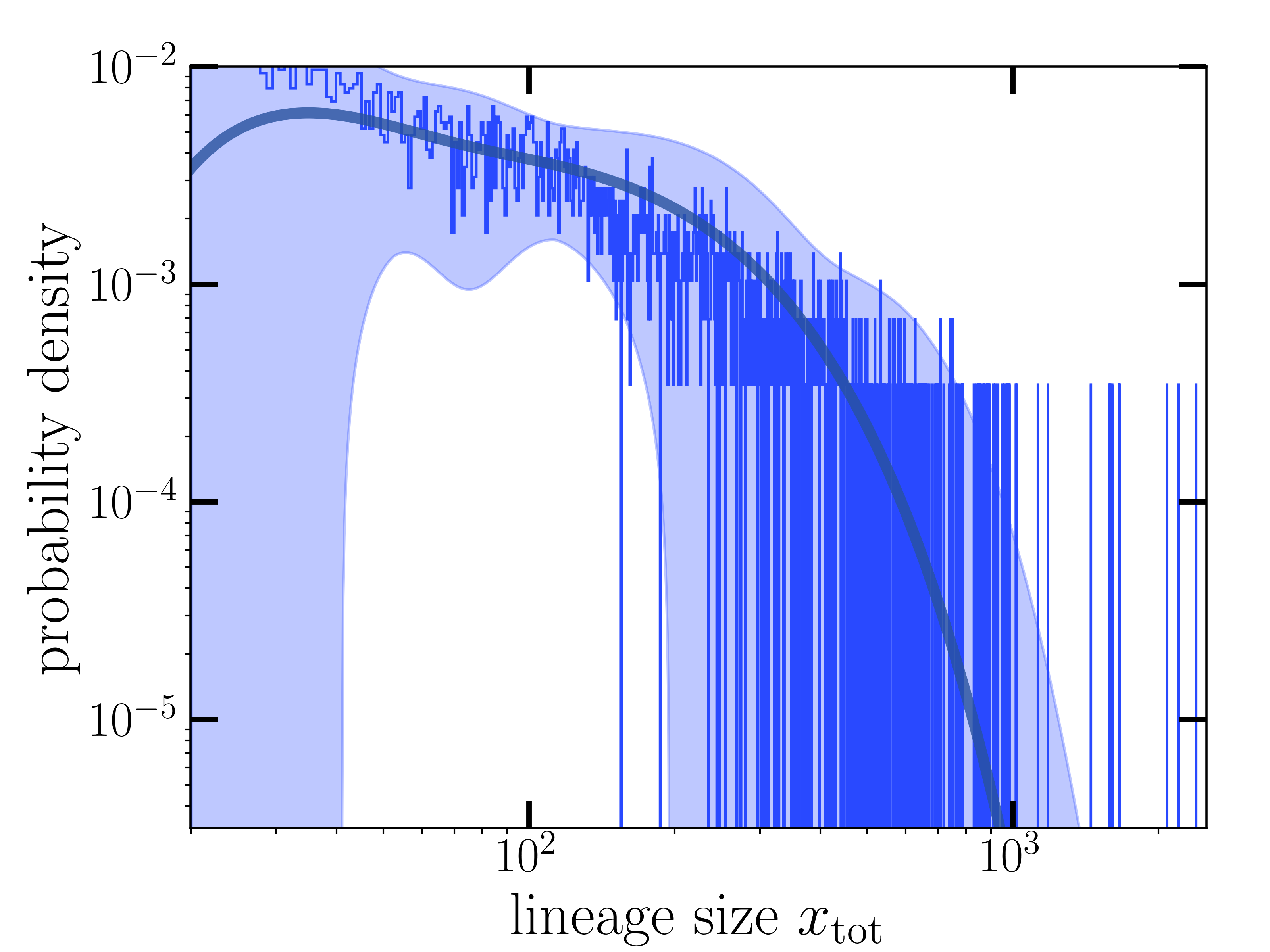
Supplementary Figure S 5: Histograms of the data for an organoid at day 16 with bin sizes 80, 1000 and 3000 compared to the SAN-model predictions for the total lineage size probability densites. Shaded areas show the uncertainties of the fitted parameters (see Table 1 of the main text).

      

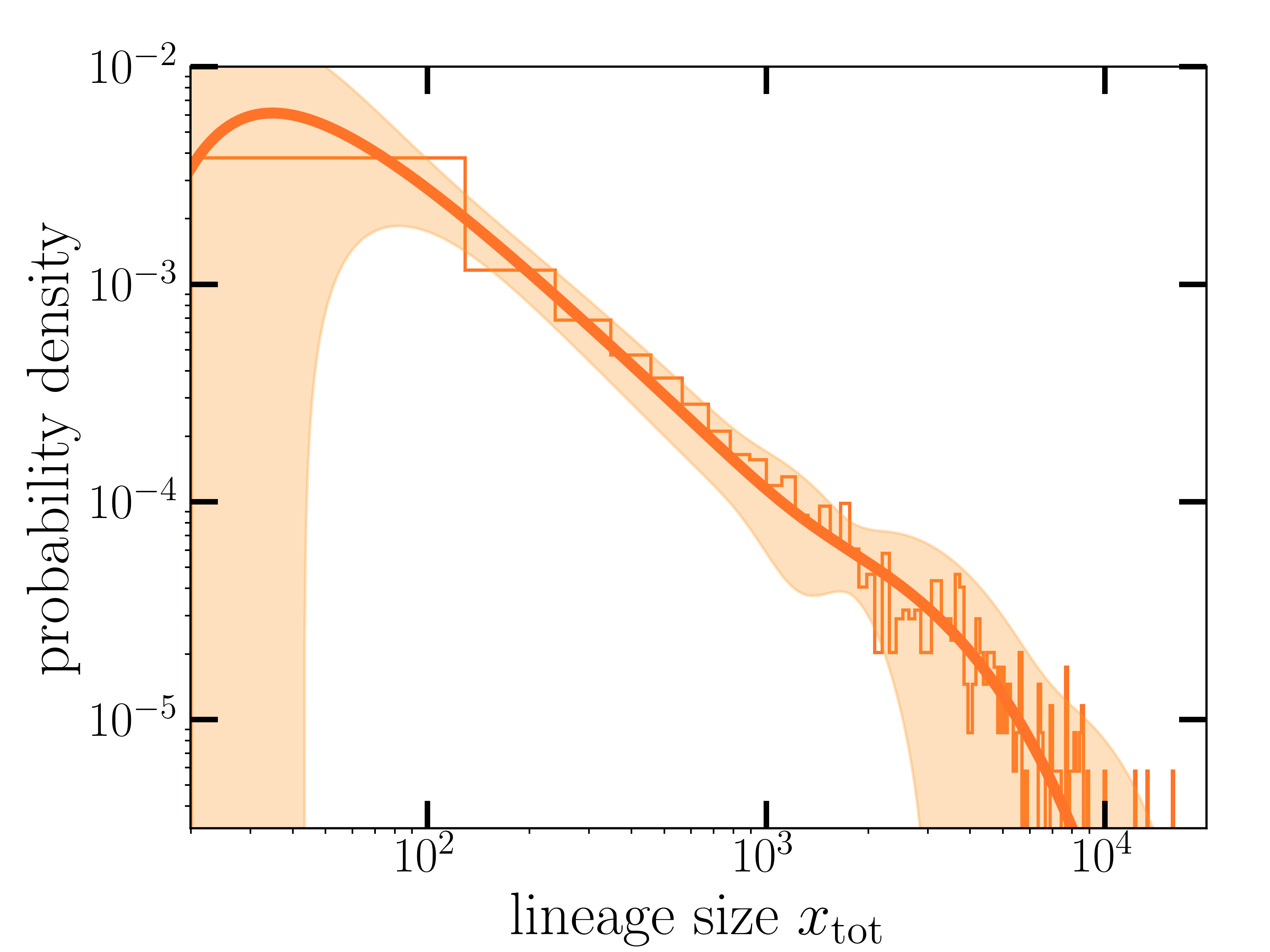
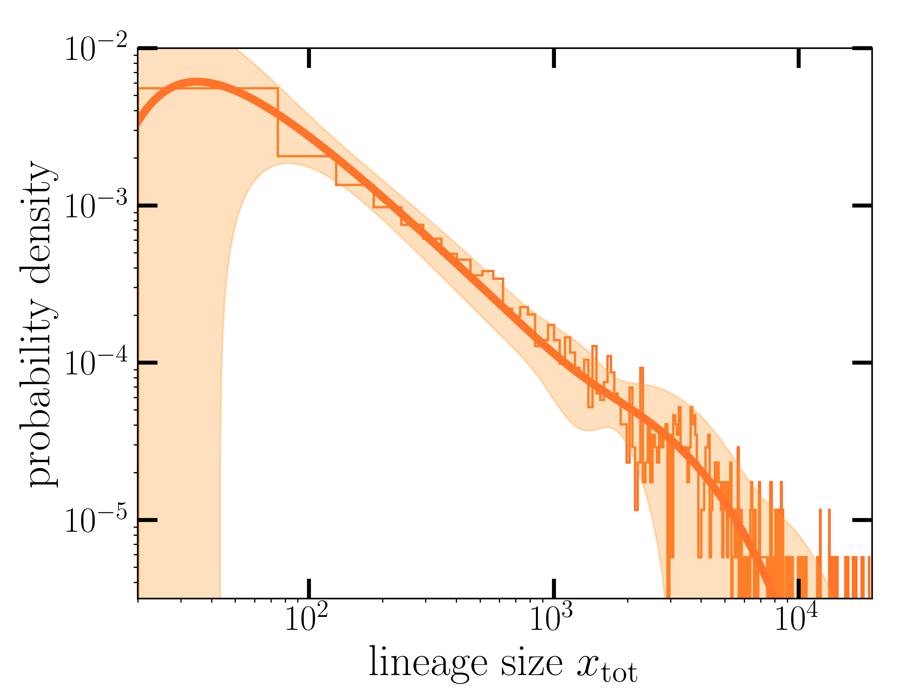
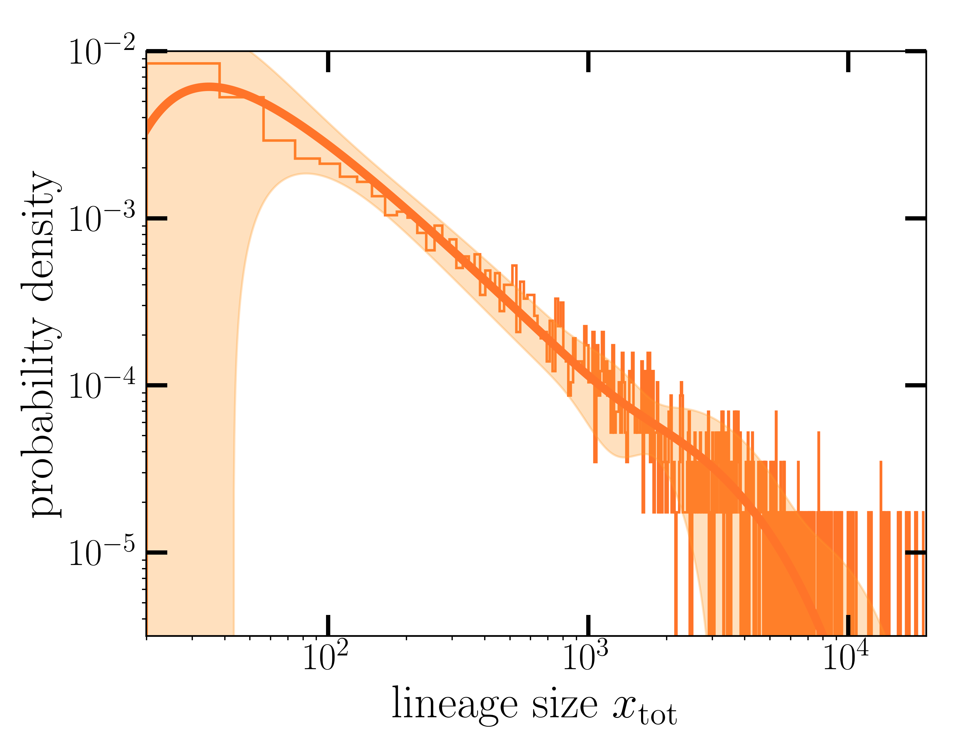
Supplementary Figure S 6: Histograms of the data for an organoid at day 40 with bin sizes 500, 1000 and 3000 compared to the SAN-model predictions for the total lineage size probability densites. Shaded areas show the uncertainties of the fitted parameters (see Table 1 of the main text).