Inverse Stochastic Optimal Control for Linear-Quadratic Gaussian and Linear-Quadratic Sensorimotor Control Models

Abstract

In this paper, we define and solve the Inverse Stochastic Optimal Control (ISOC) problem of the linear-quadratic Gaussian (LQG) and the linear-quadratic sensorimotor (LQS) control model. These Stochastic Optimal Control (SOC) models are state-of-the-art approaches describing human movements. The LQG ISOC problem consists of finding the unknown weighting matrices of the quadratic cost function and the covariance matrices of the additive Gaussian noise processes based on ground truth trajectories observed from the human in practice. The LQS ISOC problem aims at additionally finding the covariance matrices of the signal-dependent noise processes characteristic for the LQS model. We propose a solution to both ISOC problems which iteratively estimates cost function and covariance matrices via two bi-level optimizations. Simulation examples show the effectiveness of our developed algorithm. It finds parameters that yield trajectories matching mean and variance of the ground truth data.

I INTRODUCTION

Stochastic Optimal Control (SOC) models are state-of-the-art approaches describing human movements to a single goal [1]. They characterize the average behavior via the mean as well as the variability patterns via higher stochastic moments of the system state. The current main representative is the linear-quadratic (LQ) sensorimotor (LQS) control model [2, 3, 4] which builds upon the well-known LQ Gaussian (LQG) control model but takes signal-dependent noise processes in human execution and perception into account. Compared to the LQG case, in the LQS model a control-dependent noise process is added to the system state equation and a state-dependent one to the output equation. In order to verify the model hypothesis and investigate the optimality principles underlying human movements an identification of the unknown parameters of the SOC models, namely relative weights of the cost function and covariance matrices of the noise processes, on the basis of ground truth data, i.e. human measurements, is needed. The identified SOC models can then build the starting point to design a supporting automation in human-machine collaboration settings. For example, by taking advantage of the predicted human variability the accuracy of executing a via-point-movement task can be improved. In case of the LQS model, the identification of the covariance matrices is not only necessary to describe human variability patterns, like in the LQG case, but also to model human average behavior (see our results of Section II). However, research regarding the inverse problem of LQ SOC models, i.e. identifying both unknown parameter types, weighting matrices of the cost function and covariance matrices of the noise processes, is scarce.

Among the approaches considering the identification problem of SOC models, [6] address only the LQG model and thus, the influence of the signal-dependent noise processes cannot be investigated. The same holds for [7] and in addition, the proposed method determines solely cost function parameters. In [8], the control-dependent noise process is taken into account. However, a fully and not partially observable model is considered. Typically, SOC models of human movements are partially observable since not all system states can be measured by the human and its measurements are subject to noise. Moreover, in [8] only the cost function is determined. Although [9] propose an identification approach for the complete LQS control model, the covariance matrices are not estimated as well. Finally, [10] determine cost function and noise parameters of the LQS model but since the authors apply the model to describe human driving behavior, the inverse problem is not focused. Thus, a formal mathematical description of the problem is missing and only two cost and two noise parameters are estimated. Whereas this can be sufficient for the specific driving task, such few parameters fail to analyze the influence of all parameters available in a SOC model. Due to solely identifying the cost function and due to their missing consideration of the partially observable setting, the majority of known Inverse Optimal Control (IOC) methods are not applicable to the inverse problem of SOC models in their current form. They are used to identify the relative weights of different cost function candidates, penalizing e.g. jerk, torque or effort, for deterministic optimal control models of human motor planning. Bi-level optimization approaches can be found e.g. in [11, 12, 13], methods based on Karush-Kuhn-Tucker conditions in [14, 15, 16] and [17] utilize a method based on Hamilton optimality conditions. Such models assume a separation between motor planning and execution (see e.g. [18, 19] as seminal works). However, this traditional separation has been challenged in the last years [1] and SOC models arose.

In summary, the inverse problem of LQ SOC models lacks formal definitions and no method exists that solves this Inverse Stochastic Optimal Control (ISOC) problem for the LQG and LQS case. Consequently, in this paper, we first define these ISOC problems and then, propose a new algorithm that solves them by iteratively estimating cost function and noise parameters via two bi-level optimizations. For their lower level we state new recursive calculations of the stochastic moments of the system state compared in the upper level with their ground truth values which leads to significantly reduced computation times. Moreover, our algorithm considers that in the ground truth data observed from the human not all system states are measured. Lastly, we provide simulation examples to show the effectiveness of our algorithm.

II INVERSE STOCHASTIC OPTIMAL CONTROL PROBLEMS

In this section, formal definitions of the ISOC problem for the LQG (Subsection II-A) and the LQS case (Subsection II-B) are given. Based on stating the respective SOC problems and the solutions to these forward optimal control problems, the inverse problems are defined.

II-A Linear-Quadratic Gaussian Case

Let the discrete dynamics of a linear system be given by

$$\bm{x}_{t+1} =\bm{A}\bm{x}_{t}+\bm{B}\bm{u}_{t}+\bm{\xi}_{t}$$ (1)

$$\bm{y}_{t} =\bm{H}\bm{x}_{t}+\bm{\omega}_{t},$$ (2)

where $\bm{x}\in\mathbb{R}^{n}$ denotes the system state (with additional time index $t$ the corresponding stochastic process $\bm{x}_{t}$ is described), $\bm{u}\in\mathbb{R}^{m}$ the control variables, $\bm{y}\in\mathbb{R}^{r}$ the observable output and $\bm{A}$, $\bm{B}$, $\bm{H}$ system matrices of appropriate dimensions that may depend on time. Furthermore, $\bm{\xi}_{t}\in\mathbb{R}^{n}$ and $\bm{\omega}_{t}\in\mathbb{R}^{r}$ are white Gaussian noise processes independent to each other and to $\bm{x}_{t}$. Each noise process $\bm{\xi}_{t}$ and $\bm{\omega}_{t}$ is composed by a standard white Gaussian noise process $\bm{\alpha}_{t}\in\mathbb{R}^{p}$ and $\bm{\beta}_{t}\in\mathbb{R}^{q}$ ($\mathrm{cov}\left(\bm{\alpha}_{t},\bm{\alpha}_{t}\right)=\mathrm{cov}\left(\bm{\alpha}_{t}\right)=\bm{I}$ and $\mathrm{cov}\left(\bm{\beta}_{t}\right)=\bm{I}$), respectively, where $\bm{\alpha}_{t}$ and $\bm{\beta}_{t}$ are independent to each other and to $\bm{x}_{t}$: $\bm{\xi}_{t}=\bm{\Sigma}^{\bm{\xi}}\bm{\alpha}_{t}$ and $\bm{\omega}_{t}=\bm{\Sigma}^{\bm{\omega}}\bm{\beta}_{t}$. Thus, the covariance matrices of $\bm{\xi}_{t}$ and $\bm{\omega}_{t}$ are defined by $\bm{\Omega}^{\bm{\xi}}=\mathrm{cov}\left(\bm{\xi}_{t}\right)=\bm{\Sigma}^{\bm{\xi}}\left(\bm{\Sigma}^{\bm{\xi}}\right)^{\mathrm{T}}$ and $\bm{\Omega}^{\bm{\omega}}=\mathrm{cov}\left(\bm{\omega}_{t}\right)=\bm{\Sigma}^{\bm{\omega}}\left(\bm{\Sigma}^{\bm{\omega}}\right)^{\mathrm{T}}$, where $\bm{\Omega}^{\bm{\xi}}$ is assumed to be positive semi-definite and $\bm{\Omega}^{\bm{\omega}}$ positive definite. For the LQG case, we define the noise parameter vector $\bm{\sigma}\in\mathbb{R}^{\Sigma}$ as $\bm{\sigma}=\left[\begin{matrix}\operatorname{vec}(\bm{\Sigma}^{\bm{\xi}})^{\mathrm{T}}&\operatorname{vec}(\bm{\Sigma}^{\bm{\omega}})^{\mathrm{T}}\end{matrix}\right]^{\mathrm{T}}$. Finally, the initial values of $\bm{x}_{t}$ are given by $\mathrm{E}\left\{\bm{x}_{0}\right\}$ and $\bm{\Omega}^{\bm{x}}_{0}=\mathrm{cov}\left(\bm{x}_{0}\right)$ ($\bm{\Omega}^{\bm{x}}_{0}$ positive semi-definite).

Considering the LQG optimal control problem, the aim is to find an admissible control strategy for (1) and (2) that minimizes a performance criterion [20, p. 258], which is defined by

$$J=\mathrm{E}\left\{\bm{x}^{\mathrm{T}}_{N}\bm{Q}_{N}\bm{x}_{N}+\sum_{t=0}^{N-1}\bm{x}^{\mathrm{T}}_{t}\bm{Q}\bm{x}_{t}+\bm{u}^{\mathrm{T}}_{t}\bm{R}\bm{u}_{t}\right\},$$ (3)

where $\bm{Q}_{N}$, $\bm{Q}$ and $\bm{R}$ are symmetric matrices of appropriate dimensions with $\bm{Q}_{N}$, $\bm{Q}$ positive semi-definite and $\bm{R}$ positive definite. For these cost function matrices, we introduce the notations $\bm{Q}_{N}=\sum_{i=1}^{S_{N}}s_{N,i}\bm{q}_{N,i}\bm{q}_{N,i}^{\mathrm{T}}$, $\bm{Q}=\sum_{i=1}^{S_{Q}}s_{Q,i}\bm{q}_{Q,i}\bm{q}_{Q,i}^{\mathrm{T}}$ and $\bm{R}=\sum_{i=1}^{S_{R}}s_{R,i}\bm{q}_{R,i}\bm{q}_{R,i}^{\mathrm{T}}$, where $\bm{q}_{N,i},\bm{q}_{Q,i}\in\mathbb{R}^{n}$ and $\bm{q}_{R,i}\in\mathbb{R}^{m}$. For the later inverse problem definition, we define the cost function parameter vector $\bm{s}\in\mathbb{R}^{S}$ ($S=S_{N}+S_{Q}+S_{R}$) as $\bm{s}^{\mathrm{T}}=\left[\begin{matrix}s_{N,1}&\!\!\dots\!&s_{N,S_{N}}&s_{Q,1}&\!\dots\!&s_{Q,S_{Q}}&s_{R,1}&\!\dots\!&s_{R,S_{R}}\end{matrix}\right]$.

According to [20, p. 274], the LQG problem is solved by the control law $\bm{u}_{t}=-\bm{L}_{t}\hat{\bm{x}}_{t}$ with

$$\bm{L}_{t} =\left(\bm{R}+\bm{B}^{\mathrm{T}}\bm{Z}_{t+1}\bm{B}\right)^{-1}\bm{B}^{\mathrm{T}}\bm{Z}_{t+1}\bm{A}$$ (4)

and $\hat{\bm{x}}_{t}$ denoting the estimation of $\bm{x}_{t}$ calculated by $\hat{\bm{x}}_{t+1}=\bm{A}\hat{\bm{x}}_{t}+\bm{B}\bm{u}_{t}+\bm{K}_{t}\left(\bm{y}_{t}-\bm{H}\hat{\bm{x}}_{t}\right)$, where

$$\bm{K}_{t} =\bm{A}\bm{P}_{t}\bm{H}^{\mathrm{T}}\left(\bm{H}\bm{P}_{t}\bm{H}^{\mathrm{T}}+\bm{\Omega}^{\bm{\omega}}\right)^{-1}.$$ (5)

Here, $\bm{Z}_{t}$ and $\bm{P}_{t}$ are computed via Riccati difference equations with boundary values $\bm{Z}_{N}=\bm{Q}_{N}$ and $\bm{P}_{0}=\bm{\Omega}_{0}^{\bm{x}}$ [20, p. 229, p. 274].

As explained in Section I, given the control $\bm{L}_{t}$ and filter matrices $\bm{K}_{t}$, we need a recursive calculation of $\mathrm{E}\left\{\bm{x}_{t}\right\}$ and $\bm{\Omega}_{t}^{\bm{x}}=\mathrm{cov}\left(\bm{x}_{t}\right)$ for an efficient realization of the lower level of the bi-level optimizations in our ISOC algorithm later.

Lemma 1

Let the LQG control problem be defined by (1), (2) and (3). Let the solution be given by the control $\bm{L}_{t}$ (4) and filter matrices $\bm{K}_{t}$ (5). Then, the mean $\mathrm{E}\left\{\bm{x}_{t}\right\}$ and covariance $\bm{\Omega}_{t}^{\bm{x}}$ of $\bm{x}_{t}$ are computed by

$$\left[\begin{matrix}\mathrm{E}\left\{\bm{x}_{t+1}\right\}\\ \mathrm{E}\left\{\hat{\bm{x}}_{t+1}\right\}\end{matrix}\right] =\bm{\mathcal{A}}_{t}\left[\begin{matrix}\mathrm{E}\left\{\bm{x}_{t}\right\}\\ \mathrm{E}\left\{\hat{\bm{x}}_{t}\right\}\end{matrix}\right],$$ (6)

$$\left[\begin{matrix}\bm{\Omega}_{t+1}^{\bm{x}}\!\!&\bm{\Omega}_{t+1}^{\bm{x}\hat{\bm{x}}}\\ \bm{\Omega}_{t+1}^{\hat{\bm{x}}\bm{x}}\!\!&\bm{\Omega}_{t+1}^{\hat{\bm{x}}}\end{matrix}\right] =\bm{\mathcal{A}}_{t}\left[\begin{matrix}\bm{\Omega}_{t}^{\bm{x}}\!\!\!\!&\bm{\Omega}_{t}^{\bm{x}\hat{\bm{x}}}\\ \bm{\Omega}_{t}^{\hat{\bm{x}}\bm{x}}\!\!\!\!&\bm{\Omega}_{t}^{\hat{\bm{x}}}\end{matrix}\right]\bm{\mathcal{A}}^{\mathrm{T}}_{t}+\left[\begin{matrix}\bm{\Omega}^{\bm{\xi}}\!\!\!\!&\bm{0}\\ \bm{0}\!\!\!\!&\bm{K}_{t}\bm{\Omega}^{\bm{\omega}}\bm{K}^{\mathrm{T}}_{t}\end{matrix}\right]$$ (7)

with $\bm{\Omega}_{t}^{\bm{x}\hat{\bm{x}}}=\mathrm{cov}\left(\bm{x}_{t},\hat{\bm{x}}_{t}\right)$, $\bm{\Omega}_{t}^{\hat{\bm{x}}\bm{x}}=\mathrm{cov}\left(\hat{\bm{x}}_{t},\bm{x}_{t}\right)$, $\bm{\Omega}_{t}^{\hat{\bm{x}}}=\mathrm{cov}\left(\hat{\bm{x}}_{t}\right)$,

$$\bm{\mathcal{A}}_{t}=\begin{bmatrix}\bm{A}&-\bm{B}\bm{L}_{t}\\ \bm{K}_{t}\bm{H}&\bm{A}-\bm{K}_{t}\bm{H}-\bm{B}\bm{L}_{t}\end{bmatrix}$$ (8)

and initial values $\mathrm{E}\left\{\hat{\bm{x}}_{0}\right\}=\hat{\bm{x}}_{0}=\mathrm{E}\left\{\bm{x}_{0}\right\}$ and

$$\left[\begin{matrix}\bm{\Omega}_{0}^{\bm{x}}\!\!\!\!&\bm{\Omega}_{0}^{\bm{x}\hat{\bm{x}}}\\ \bm{\Omega}_{0}^{\hat{\bm{x}}\bm{x}}\!\!\!\!&\bm{\Omega}_{0}^{\hat{\bm{x}}}\end{matrix}\right]=\left[\begin{matrix}\bm{\Omega}_{0}^{\bm{x}}&\bm{0}\\ \bm{0}&\bm{0}\end{matrix}\right].$$ (9)

Proof.

With $\bm{u}_{t}=-\bm{L}_{t}\hat{\bm{x}}_{t}$ in (1) and in the filter equation for $\hat{\bm{x}}_{t+1}$, (6) results. Using the same expressions for $\bm{x}_{t+1}$ and $\hat{\bm{x}}_{t+1}$ in

$$\left[\begin{matrix}\bm{\Omega}_{t+1}^{\bm{x}}\!\!&\bm{\Omega}_{t+1}^{\bm{x}\hat{\bm{x}}}\\ \bm{\Omega}_{t+1}^{\hat{\bm{x}}\bm{x}}\!\!&\bm{\Omega}_{t+1}^{\hat{\bm{x}}}\end{matrix}\right]=\mathrm{cov}\left(\left[\begin{matrix}\bm{x}_{t+1}\\ \hat{\bm{x}}_{t+1}\end{matrix}\right]\right)$$ (10)

(7) is obtained by considering the independence of the noise processes $\bm{\xi}_{t}$ and $\bm{\omega}_{t}$ between each other and to $\bm{x}_{t}$ as well as $\hat{\bm{x}}_{t}$. The initial values follow from the initial value $\bm{\Omega}_{0}^{\bm{x}}$ of $\bm{x}_{t}$ and the initialization of the filter equations with $\hat{\bm{x}}_{0}=\mathrm{E}\left\{\bm{x}_{0}\right\}$.

Lemma 1 yields that the average behavior $\mathrm{E}\left\{\bm{x}_{t}\right\}$ predicted by the LQG model is solely influenced by the cost function parameters $\bm{s}$, which can be seen by (6) and (4), since $\bm{L}_{t}$ is independent of the covariance matrices. This is a special property of the LQG model due to the separation theorem. In the next subsection, we show that in the LQS case the covariance matrices are necessary to compute the average behavior as well.

Now, we can define the ISOC problem for the LQG case.

Assumption 1

Suppose a set $\{{\bm{M}\bm{x}^{\ast}_{t}}^{(k)}\}$ ($k\in\{1,\dots,K\}$) of time-discrete trajectories ${\bm{M}\bm{x}^{\ast}_{t}}^{(k)}$ is given, where ${\bm{x}^{\ast}_{t}}^{(k)}$ denotes a realization of the stochastic process $\bm{x}_{t}^{\ast}$ and $\bm{M}\in\mathbb{R}^{\bar{n}\times n}$ follows from the identity matrix $\bm{I}$ by deleting rows corresponding to states which are not measured in the ground truth data. The stochastic process $\bm{x}_{t}^{\ast}$ results from the estimation-control loop consisting of (1) and (2) with $\bm{L}_{t}^{\ast}$ (4) and $\bm{K}_{t}^{\ast}$ (5) corresponding to unknown cost function $\bm{s}^{\ast}$ and noise parameters $\bm{\sigma}^{\ast}$. Furthermore, let $\hat{\bm{m}}_{t}\approx\mathrm{E}\left\{\bm{M}\bm{x}_{t}^{\ast}\right\}$ and $\hat{\bm{\Omega}}^{\bm{x}^{\ast}}_{t}\approx\bm{M}\bm{\Omega}^{\bm{x}^{\ast}}_{t}\bm{M}^{\mathrm{T}}$ be estimates of the mean and covariance of the measured states of $\bm{x}_{t}^{\ast}$ computed from the set of trajectories.

Assumption 2

It is known which elements of $\bm{\sigma}^{\ast}$ are non-zero, but not their exact numerical values. Furthermore, the basis vectors $\bm{q}_{N,i}$, $\bm{q}_{Q,i}$ and $\bm{q}_{R,i}$ corresponding to the non-zero coefficients in $\bm{s}^{\ast}$ are known. Moreover, the system matrices $\bm{A}$, $\bm{B}$ and $\bm{H}$ are known.

Problem 1

Let Assumptions 1 and 2 hold. Find parameters $\tilde{\bm{s}}$ and $\tilde{\bm{\sigma}}$ such that $\tilde{\bm{L}}_{t}$ (4) and $\tilde{\bm{K}}_{t}$ (5) resulting from $\tilde{\bm{s}}$ and $\tilde{\bm{\sigma}}$ lead to $\tilde{\bm{x}}_{t}$ in the estimation-control loop ((1) and (2) with $\tilde{\bm{L}}_{t}$ and $\tilde{\bm{K}}_{t}$) with $\mathrm{E}\left\{\bm{M}\tilde{\bm{x}}_{t}\right\}=\mathrm{E}\left\{\bm{M}\bm{x}^{\ast}_{t}\right\}$ and $\bm{M}\bm{\Omega}^{\tilde{\bm{x}}}_{t}\bm{M}^{\mathrm{T}}=\bm{M}\bm{\Omega}^{\bm{x}^{\ast}}_{t}\bm{M}^{\mathrm{T}}$.

Remark 1

Assumption 1 defines the ground truth data for an ISOC algorithm solving Problem 1. In a practical setup, these ground truth data is observed from the human. In Assumption 1, $\bm{M}$ takes into account that not all system states can be measured in general. In addition, in several models of human biomechanics (see e.g. Section IV) the human control signal as well as the perceived output are only virtual quantities and thus not measured when a human is observed. Hence, we do not consider measurements of realizations of $\bm{u}^{\ast}_{t}$ or $\bm{y}^{\ast}_{t}$ and do not aim at finding parameters $\tilde{\bm{s}}$ and $\tilde{\bm{\sigma}}$ yielding matching mean and covariance of the control or output variables as well.

II-B Linear-Quadratic Sensorimotor Case

The LQG model cannot fully account for the characteristic variability patterns of human movements [2, 10]. Hereto, a control-dependent noise process $\sum_{i=1}^{c}\varepsilon_{t}^{(i)}\bm{C}_{i}\bm{u}_{t}$ considering that higher control magnitudes lead to higher motor noise and a state-dependent noise process $\sum_{i=1}^{d}\epsilon_{t}^{(i)}\bm{D}_{i}\bm{x}_{t}$ accounting for multiplicative noise in human perception need to be added to (1) and (2) [4]:

$$\bm{x}_{t+1} =\bm{A}\bm{x}_{t}+\bm{B}\bm{u}_{t}+\bm{\xi}_{t}+\sum_{i=1}^{c}\varepsilon_{t}^{(i)}\bm{C}_{i}\bm{u}_{t}$$ (11)

$$\bm{y}_{t} =\bm{H}\bm{x}_{t}+\bm{\omega}_{t}+\sum_{i=1}^{d}\epsilon_{t}^{(i)}\bm{D}_{i}\bm{x}_{t},$$ (12)

where $\bm{x}$, $\bm{u}$, $\bm{y}$, $\bm{A}$, $\bm{B}$, $\bm{H}$, $\bm{\xi}_{t}$ and $\bm{\omega}_{t}$ are defined as in Subsection II-A. The time-independent matrices $\bm{C}_{i}$ and $\bm{D}_{i}$ are composed by $\bm{C}_{i}=\sigma_{i}^{\bm{u}}\bm{B}\bm{F}_{i}$ and $\bm{D}_{i}=\sigma_{i}^{\bm{x}}\bm{H}\bm{G}_{i}$, respectively, where $\bm{C}_{i}$, $\bm{D}_{i}$, $\bm{F}_{i}$ and $\bm{G}_{i}$ have appropriate dimensions. Furthermore, $\bm{\varepsilon}_{t}=\left[\begin{matrix}\varepsilon_{t}^{(1)}&\dots&\varepsilon_{t}^{(c)}\end{matrix}\right]^{\mathrm{T}}$ and $\bm{\epsilon}_{t}=\left[\begin{matrix}\epsilon_{t}^{(1)}&\dots&\epsilon_{t}^{(d)}\end{matrix}\right]^{\mathrm{T}}$ are standard white Gaussian noise processes ($\mathrm{cov}\left(\bm{\varepsilon}_{t}\right)=\mathrm{cov}\left(\bm{\epsilon}_{t}\right)=\bm{I}$) independent to each other, $\bm{\xi}_{t}$, $\bm{\omega}_{t}$ and $\bm{x}_{t}$. For the LQS case, we define the noise parameter vector $\bm{\sigma}\in\mathbb{R}^{\Sigma}$ as $\bm{\sigma}=\left[\begin{matrix}\operatorname{vec}(\bm{\Sigma}^{\bm{\xi}})^{\mathrm{T}}&\operatorname{vec}(\bm{\Sigma}^{\bm{\omega}})^{\mathrm{T}}&\sigma_{1}^{\bm{u}}&\dots&\sigma_{c}^{\bm{u}}&\sigma_{1}^{\bm{x}}&\dots&\sigma_{d}^{\bm{x}}\end{matrix}\right]^{\mathrm{T}}$.

According to [4], the separation theorem no longer holds and one can compute an approximate (suboptimal) solution to the forward problem (minimization of (3) subject to (11) and (12)) consisting of the control law $\bm{u}_{t}=-\bm{L}_{t}\hat{\bm{x}}_{t}$ and estimator law $\hat{\bm{x}}_{t+1}=\bm{A}\hat{\bm{x}}_{t}+\bm{B}\bm{u}_{t}+\bm{K}_{t}\left(\bm{y}_{t}-\bm{H}\hat{\bm{x}}_{t}\right)+\bm{\eta}_{t}$ by iterating between

$$\bm{L}_{t} =\Big{(}\bm{R}+\bm{B}^{\mathrm{T}}\bm{Z}_{t+1}^{\bm{x}}\bm{B}$$

$$\hphantom{=}+\sum_{i}\bm{C}_{i}^{\mathrm{T}}\left(\bm{Z}_{t+1}^{\bm{x}}+\bm{Z}_{t+1}^{\bm{e}}\right)\bm{C}_{i}\Big{)}^{-1}\bm{B}^{\mathrm{T}}\bm{Z}_{t+1}^{\bm{x}}\bm{A}$$ (13)

and

$$\bm{K}_{t} =\bm{A}\bm{P}_{t}^{\bm{e}}\bm{H}^{\mathrm{T}}\Big{(}\bm{H}\bm{P}_{t}^{\bm{e}}\bm{H}^{\mathrm{T}}+\bm{\Omega}^{\bm{\omega}}$$

$$\hphantom{=}+\sum_{i}\bm{D}_{i}\left(\bm{P}_{t}^{\bm{e}}+\bm{P}_{t}^{\hat{\bm{x}}}+\bm{P}_{t}^{\hat{\bm{x}}\bm{e}}+\bm{P}_{t}^{\bm{e}\hat{\bm{x}}}\right)\bm{D}_{i}^{\mathrm{T}}\Big{)}^{-1}$$ (14)

starting with an initial estimate for $\bm{K}_{t}$. The recursive equations to compute $\bm{Z}_{t}^{\bm{x}}$, $\bm{Z}_{t}^{\bm{e}}$, $\bm{P}_{t}^{\bm{e}}$, $\bm{P}_{t}^{\hat{\bm{x}}}$, $\bm{P}_{t}^{\hat{\bm{x}}\bm{e}}$ and $\bm{P}_{t}^{\bm{e}\hat{\bm{x}}}$ can be found in [4]. The white Gaussian noise process $\bm{\eta}_{t}\in\mathbb{R}^{n}$ has the symmetric and positive semi-definite covariance matrix $\bm{\Omega}^{\bm{\eta}}$ and is independent to all other stochastic processes. This noise process accounts for errors of the internal model used by the human for signal processing [10]. However, since its characteristics are unexplored until now, we omit $\bm{\eta}_{t}$ in our ISOC algorithm and do not include the parameters of $\bm{\Omega}^{\bm{\eta}}$ in $\bm{\sigma}$. This would be possible by following the procedure of $\bm{\xi}_{t}$ and $\bm{\omega}_{t}$ for $\bm{\eta}_{t}$.

Again, we state a recursive calculation of $\mathrm{E}\left\{\bm{x}_{t}\right\}$ and $\bm{\Omega}_{t}^{\bm{x}}$ for our ISOC algorithm later.

Lemma 2

Let the LQS control problem be defined by (11), (12) and (3). Let the (approximate) solution be given by $\bm{L}_{t}$ (13) and $\bm{K}_{t}$ (14). Then, the mean $\mathrm{E}\left\{\bm{x}_{t}\right\}$ and covariance $\bm{\Omega}_{t}^{\bm{x}}$ of $\bm{x}_{t}$ are computed by

$$\left[\begin{matrix}\mathrm{E}\left\{\bm{x}_{t+1}\right\}\\ \mathrm{E}\left\{\hat{\bm{x}}_{t+1}\right\}\end{matrix}\right] =\bm{\mathcal{A}}_{t}\left[\begin{matrix}\mathrm{E}\left\{\bm{x}_{t}\right\}\\ \mathrm{E}\left\{\hat{\bm{x}}_{t}\right\}\end{matrix}\right],$$ (15)

$$\left[\begin{matrix}\bm{\Omega}_{t+1}^{\bm{x}}\!\!&\bm{\Omega}_{t+1}^{\bm{x}\hat{\bm{x}}}\\ \bm{\Omega}_{t+1}^{\hat{\bm{x}}\bm{x}}\!\!&\bm{\Omega}_{t+1}^{\hat{\bm{x}}}\end{matrix}\right] =\bm{\mathcal{A}}_{t}\left[\begin{matrix}\bm{\Omega}_{t}^{\bm{x}}\!\!\!\!&\bm{\Omega}_{t}^{\bm{x}\hat{\bm{x}}}\\ \bm{\Omega}_{t}^{\hat{\bm{x}}\bm{x}}\!\!\!\!&\bm{\Omega}_{t}^{\hat{\bm{x}}}\end{matrix}\right]\bm{\mathcal{A}}^{\mathrm{T}}_{t}$$

$$\hphantom{=}+\left[\begin{matrix}\bm{\Omega}^{\bm{\xi}}\!\!\!\!&\bm{0}\\ \bm{0}\!\!\!\!&\bm{\Omega}^{\bm{\eta}}+\bm{K}_{t}\bm{\Omega}^{\bm{\omega}}\bm{K}^{\mathrm{T}}_{t}\end{matrix}\right]+\left[\begin{matrix}\bar{\bm{\Omega}}_{t}^{\hat{\bm{x}}}\!\!\!\!&\bm{0}\\ \bm{0}\!\!\!\!&\bar{\bm{\Omega}}_{t}^{\bm{x}}\end{matrix}\right]$$ (16)

with $\bar{\bm{\Omega}}_{t}^{\hat{\bm{x}}}=\sum_{i}\bm{C}_{i}\bm{L}_{t}\left(\bm{\Omega}_{t}^{\hat{\bm{x}}}+\mathrm{E}\left\{\hat{\bm{x}}_{t}\right\}\mathrm{E}\left\{\hat{\bm{x}}_{t}\right\}^{\mathrm{T}}\right)\bm{L}_{t}^{\mathrm{T}}\bm{C}_{i}^{\mathrm{T}}$, $\bar{\bm{\Omega}}_{t}^{\bm{x}}=\sum_{i}\bm{K}_{t}\bm{D}_{i}\left(\bm{\Omega}_{t}^{\bm{x}}+\mathrm{E}\left\{\bm{x}_{t}\right\}\mathrm{E}\left\{\bm{x}_{t}\right\}^{\mathrm{T}}\right)\bm{D}_{i}^{\mathrm{T}}\bm{K}_{t}^{\mathrm{T}}$, $\bm{\mathcal{A}}_{t}$ (8) and initial values $\mathrm{E}\left\{\hat{\bm{x}}_{0}\right\}=\hat{\bm{x}}_{0}=\mathrm{E}\left\{\bm{x}_{0}\right\}$ and (9).

Proof.

See Appendix.

Lemma 2 yields that the average behavior $\mathrm{E}\left\{\bm{x}_{t}\right\}$ predicted by the LQS model depends on the covariance matrices and thus noise parameters $\bm{\sigma}$ since the calculation of $\bm{L}_{t}$ (13) depends on the $\bm{C}_{i}$ and $\bm{K}_{t}$ which in turn depend on $\bm{\sigma}$. Hence, the identification of the noise parameters are not only necessary for describing the variability patterns of human movements but also its average behavior.

Now, the ISOC problem of the LQS case can be defined.

Assumption 3

Assumption 1 holds with $\bm{x}^{\ast}_{t}$ being the stochastic process of the system state in the estimation-control loop consisting of (11) and (12) with $\bm{L}^{\ast}_{t}$ (13) and $\bm{K}^{\ast}_{t}$ (14) resulting from unknown cost function $\bm{s}^{\ast}$ and noise parameters $\bm{\sigma}^{\ast}$.

Assumption 4

Assumption 2 holds. Furthermore, the $c$ scaling matrices $\bm{F}_{i}$ and the $d$ scaling matrices $\bm{G}_{i}$ are known.

Problem 2

Let Assumptions 3 and 4 hold. Find parameters $\tilde{\bm{s}}$ and $\tilde{\bm{\sigma}}$ such that $\tilde{\bm{L}}_{t}$ (13) and $\tilde{\bm{K}}_{t}$ (14) resulting from $\tilde{\bm{s}}$ and $\tilde{\bm{\sigma}}$ lead to $\tilde{\bm{x}}_{t}$ in the estimation-control loop ((11) and (12) with $\tilde{\bm{L}}_{t}$ and $\tilde{\bm{K}}_{t}$) with $\mathrm{E}\left\{\bm{M}\tilde{\bm{x}}_{t}\right\}=\mathrm{E}\left\{\bm{M}\bm{x}^{\ast}_{t}\right\}$ and $\bm{M}\bm{\Omega}^{\tilde{\bm{x}}}_{t}\bm{M}^{\mathrm{T}}=\bm{M}\bm{\Omega}^{\bm{x}^{\ast}}_{t}\bm{M}^{\mathrm{T}}$.

III SOLVING ISOC PROBLEMS: A BI-LEVEL-BASED APPROACH

In order to solve both ISOC problems stated in the previous section, we propose a new algorithm in the following. Before its detailed definition is given in Subsection III-B, we describe the general approach in Subsection III-A.

III-A General Approach

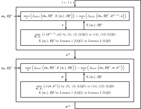
Figure 1: Overview of our ISOC algorithm.

In the following, we explain the general procedure of our ISOC algorithm shown in Fig. 1. Starting with a set of ground truth trajectories according to Assumptions 1 and 3, we state a direct optimization problem for finding parameters $\tilde{\bm{s}}$ and $\tilde{\bm{\sigma}}$. Hereto, we introduce a performance criterion $J_{\operatorname{ISOC}}$ describing how well the mean $\mathrm{E}\left\{\bm{x}_{t}\right\}$ and covariance value $\bm{\Omega}^{\bm{x}}_{t}$ of a current guess of $\bm{s}$ and $\bm{\sigma}$ match $\hat{\bm{m}}_{t}$ and $\hat{\bm{\Omega}}^{\bm{x}^{\ast}}_{t}$. In our case, we propose $J_{\operatorname{ISOC}}$ as follows:

$$J_{\operatorname{ISOC}}=\frac{\bm{w}_{\cdot,\text{m}}^{\mathrm{T}}\bm{m}^{\text{VAF}}+\bm{w}_{\cdot,\text{v}}^{\mathrm{T}}\operatorname{vec}\left(\bm{\Omega}^{\text{VAF}}\right)}{\left\lVert\bm{w}_{\cdot,\text{m}}\right\rVert_{1}+\left\lVert\bm{w}_{\cdot,\text{v}}\right\rVert_{1}},$$ (17)

where $\bm{w}_{\cdot,\text{m}}\in\mathbb{R}^{\bar{n}}$ and $\bm{w}_{\cdot,\text{v}}\in\mathbb{R}^{\bar{n}\bar{n}}$ denote weighting vectors of the variance accounted for (VAF) metric of mean and covariance, respectively. Hence, each element $m^{\text{VAF}}_{i}$ of $\bm{m}^{\text{VAF}}\in\mathbb{R}^{\bar{n}}$ is computed by

$$m^{\text{VAF}}_{i}=\left(1-\frac{\sum_{t=0}^{N}\left(\left(\mathrm{E}\left\{\bm{M}\bm{x}_{t}\right\}\right)_{i}-\hat{m}_{i,t}\right)^{2}}{\sum_{t=0}^{N}\left(\hat{m}_{i,t}-\frac{1}{N+1}\sum_{t}\hat{m}_{i,t}\right)^{2}}\right)$$ (18)

and each element $\Omega_{ij}^{\text{VAF}}$ of $\bm{\Omega}^{\text{VAF}}\in\mathbb{R}^{\bar{n}\times\bar{n}}$ by

$$\Omega^{\text{VAF}}_{ij}=\left(1-\frac{\sum_{t=0}^{N}\left(\left(\bm{M}\bm{\Omega}^{\bm{x}}_{t}\bm{M}^{\mathrm{T}}\right)_{ij}-\hat{\Omega}_{ij,t}^{\bm{x}^{\ast}}\right)^{2}}{\sum_{t=0}^{N}\left(\hat{\Omega}_{ij,t}^{\bm{x}^{\ast}}-\frac{1}{N+1}\sum_{t}\hat{\Omega}_{ij,t}^{\bm{x}^{\ast}}\right)^{2}}\right).$$ (19)

Due to the chosen VAF metric, $m^{\text{VAF}}_{i}\in(-\infty,1]$ and $\Omega^{\text{VAF}}_{ij}\in(-\infty,1]$ hold where a value of $1$ corresponds to a perfect fit between the mean or covariance resulting from the current guess of $\bm{s}$ and $\bm{\sigma}$ and the mean or covariance of the ground truth data. In $J_{\operatorname{ISOC}}$ (17), the weighting vectors $\bm{w}_{\cdot,\text{m}}\in\mathbb{R}^{\bar{n}}$ and $\bm{w}_{\cdot,\text{v}}\in\mathbb{R}^{\bar{n}\bar{n}}$ enable a varying weighting between mean and covariance VAF values as well as between these values of different states. The denominator in (17) ensures that $J_{\operatorname{ISOC}}\in(-\infty,1]$ still holds. Hence, the direct optimization aims at maximizing $J_{\operatorname{ISOC}}$: $\max\limits_{\bm{s},\bm{\sigma}}\left(J_{\operatorname{ISOC}}\left(\hat{\bm{m}}_{t},\hat{\bm{\Omega}}^{\bm{x}^{\ast}}_{t},\mathrm{E}\left\{\bm{x}_{t}\right\},\bm{\Omega}^{\bm{x}}_{t}\right)\right)=\max\limits_{\bm{s},\bm{\sigma}}\left(J_{\operatorname{ISOC}}\left(\hat{\bm{m}}_{t},\hat{\bm{\Omega}}^{\bm{x}^{\ast}}_{t},\bm{\sigma},\bm{s}\right)\right)$. In order to evaluate $J_{\operatorname{ISOC}}$, $\mathrm{E}\left\{\bm{x}_{t}\right\}$ and $\bm{\Omega}_{t}$ need to be calculated for a current guess of $\bm{s}$ and $\bm{\sigma}$ which requires the computation of the solution to the forward optimal control problem. Hence, for the optimization problem a typical bi-level-based structure results which are common in deterministic IOC as well (see e.g. [22]). In order to facilitate the computability of the bi-level-based optimization problem, we introduce an alternating descent approach motivated by the natural division of the optimization variables into cost function $\bm{s}$ and noise parameters $\bm{\sigma}$[23]. Computing the best estimate $\tilde{\bm{s}}^{(l)}$ for a given estimate $\tilde{\bm{\sigma}}^{(l-1)}$ and the best estimate $\tilde{\bm{\sigma}}^{(l)}$ for $\tilde{\bm{s}}^{(l)}$ in each iteration $l$ yields the iterative scheme shown in Fig. 1. In each of the two steps in one iteration $l$ a bi-level optimization problem results. The upper level is solved via a derivative-free optimization method to circumvent computationally expensive and maybe unreliable approximations of derivatives. For our algorithm proposed in this paper, we introduce a specially designed grid search in the next subsection. Due to the existence of a huge amount of local minima in such direct IOC optimization problems, a global optimization method is chosen. For the lower level, the results of Section II are used. With a given $\bm{s}$ and $\bm{\sigma}$ that need to be evaluated in the upper level, $\bm{K}_{t}$ and $\bm{L}_{t}$ are computed via (5) and (4) (LQG model) or (14) and (13) (LQS model). Then, our newly introduced Lemma 1 (LQG model) and Lemma 2 (LQS model) lead to $\mathrm{E}\left\{\bm{x}_{t}\right\}$ and $\bm{\Omega}^{\bm{x}}_{t}$.

Remarkably, our algorithm omits a preparation step, where filter or control matrices are identified on the basis of the ground truth trajectories first, e.g. as necessary for the inverse algorithm for the LQG control model in [6].

III-B Grid-Search-based Bi-Level Inverse Stochastic Optimal Control Algorithm

Input: $\hat{\bm{m}}_{t}$, $\hat{\bm{\Omega}}_{t}^{\bm{x}^{\ast}}$, $[a_{\sigma_{i}},\,b_{\sigma_{i}}],\forall i\in\{1,\dots,\Sigma\}$, $[a_{s_{i}},\,b_{s_{i}}],\forall i\in\{1,\dots,S\}$, $\bar{\gamma}_{l}$, $l_{\max}$

Output: $\tilde{\bm{\sigma}}$, $\tilde{\bm{s}}$

Set $l=1$

Set $\tilde{\sigma}_{i}^{(0)}=0,\forall i\in\{1,\dots,\Sigma\}$ (yields $\tilde{\bm{\sigma}}^{(0)}$)

Set $\tilde{s}_{i}^{(0)}=\frac{a_{s_{i}}+b_{s_{i}}}{2},\forall i\in\{1,\dots,S\}$ (yields $\tilde{\bm{s}}^{(0)}$)

repeat

     Determine $\tilde{\bm{s}}^{(l)}$ subject to $\tilde{\bm{\sigma}}^{(l-1)}$:

         Apply Algorithm 2 with $\bm{\theta}^{(0)}=\tilde{\bm{s}}^{(l-1)}$ and $\bm{\lambda}=\tilde{\bm{\sigma}}^{(l-1)}$ to get $\tilde{\bm{s}}^{(l)}=\bm{\theta}^{\ast}$

    Determine $\tilde{\bm{\sigma}}^{(l)}$ subject to $\tilde{\bm{s}}^{(l)}$:

         Apply Algorithm 2 with $\bm{\theta}^{(0)}=\tilde{\bm{\sigma}}^{(l-1)}$ and $\bm{\lambda}=\tilde{\bm{s}}^{(l)}$ to get $\tilde{\bm{\sigma}}^{(l)}=\bm{\theta}^{\ast}$

    $b_{s_{i}}=\frac{1}{\bar{\gamma}_{l}}\left(b_{s_{i}}+\bar{\gamma}_{l}a_{s_{i}}-a_{s_{i}}\right),\forall i\in\{1,\dots,S\}$

     $b_{\sigma_{i}}=\frac{1}{\bar{\gamma}_{l}}\left(b_{\sigma_{i}}+\bar{\gamma}_{l}a_{\sigma_{i}}-a_{\sigma_{i}}\right),\forall i\in\{1,\dots,\Sigma\}$

     $l\leftarrow l+1$

    

until $l>l_{\max}$

return $\tilde{\bm{\sigma}}=\tilde{\bm{\sigma}}^{(l_{\max})}$, $\tilde{\bm{s}}=\tilde{\bm{s}}^{(l_{\max})}$

Algorithm 1 Bi-Level-based Inverse Stochastic Optimal Control.

Input: $\hat{\bm{m}}_{t}$, $\hat{\bm{\Omega}}_{t}^{\bm{x}^{\ast}}$, $\bm{\theta}^{(0)}$, $\bm{\lambda}$, $[a_{\theta_{i}},\,b_{\theta_{i}}],\forall i\in\{1,\dots,\Theta\}$, $\mathcal{N}_{\bm{\theta}}$, $\bm{w}_{\bm{\theta},\text{m}}$, $\bm{w}_{\bm{\theta},\text{v}}$, $\mathcal{P}_{\bm{\theta}}$, $\bar{\gamma}_{\theta}$, $\delta_{\gamma,\bm{\theta}}$, $\delta_{\bm{\theta}}$, $v_{\bm{\theta},\max}$

Output: $\bm{\theta}^{\ast}$

Set $v=1$, $\gamma=2$

Set $j_{\max}=1$, $J_{\operatorname{ISOC}}^{(j_{\max}),(0)}=J_{\operatorname{ISOC}}^{(j_{\max}),(-1)}=-\infty$

repeat

     foreach $p\in\mathcal{P}_{\bm{\theta}}$ do

         Initialize search space:

             $a_{\theta_{i}}^{(v)}=\max\big{(}0,\theta_{i}^{(v-1)}-\frac{b_{\theta_{i}}-a_{\theta_{i}}}{\gamma}\big{)},\forall\theta_{i}\in p$

             $b_{\theta_{i}}^{(v)}=\theta_{i}^{(v-1)}+\frac{b_{\theta_{i}}-a_{\theta_{i}}}{\gamma},\forall\theta_{i}\in p$

             $\begin{aligned} \mathcal{M}_{\theta_{i}}&=\bigg{\{}a_{\theta_{i}}^{(v)},\,a_{\theta_{i}}^{(v)}+\frac{1}{\mathcal{N}_{\bm{\theta}}-1}\left(b_{\theta_{i}}^{(v)}-a_{\theta_{i}}^{(v)}\right),\dots,\\ &\hphantom{=}a_{\theta_{i}}^{(v)}+\frac{\mathcal{N}_{\bm{\theta}}-2}{\mathcal{N}_{\bm{\theta}}-1}\left(b_{\theta_{i}}^{(v)}-a_{\theta_{i}}^{(v)}\right),\,b_{\theta_{i}}^{(v)}\bigg{\}},\forall\theta_{i}\in p\end{aligned}$

             $\mathcal{M}_{\theta_{i}}=\{\theta_{i}^{(v-1)}\},\forall\theta_{i}\notin p$

            

        Initialize search grid:

             Define $\mathcal{G}^{(v)}$ as the set of $\mathcal{N}_{\bm{\theta}}^{\lvert p\rvert}$ different vectors $\bar{\bm{\theta}}^{(j)}$, where $\bar{\theta}^{(j)}_{i}\in\mathcal{M}_{\theta_{i}}$ ($\forall i\in\{1,\dots,\Theta\}$) holds for their elements

            

        Evaluate forward solution at grid points:

             for $j=1,\,2,\,\dots,\,\mathcal{N}_{\bm{\theta}}^{\lvert p\rvert}$ do

                 Determine $\bm{K}_{t}$ and $\bm{L}_{t}$ with $\bm{\lambda}$ and $\bar{\bm{\theta}}^{(j)}\in\mathcal{G}^{(v)}$ by (5), (4) (LQG) or (14), (13) (LQS)

                 Determine $\mathrm{E}\left\{\bm{x}_{t}\right\}$ and $\bm{\Omega}_{t}^{\bm{x}}$ by Lemma 1 (LQG) or Lemma 2 (LQS)

                 Determine $J_{\operatorname{ISOC}}^{(j),(v)}$ with $\bm{w}_{\bm{\theta},\text{m}}$ and $\bm{w}_{\bm{\theta},\text{v}}$ by (17) using $\mathrm{E}\left\{\bm{x}_{t}\right\}$ and $\bm{\Omega}_{t}^{\bm{x}}$

                

            

        Determine $j_{\max}$:

             $j_{\max}=\arg\max\limits_{j}\left(J_{\operatorname{ISOC}}^{(j),(v)}\right)$

             $\bm{\theta}^{(v)}=\bar{\bm{\theta}}^{(j_{\max})}$

            

        

    if $\lvert J_{\operatorname{ISOC}}^{(j_{\max}),(v)}-J_{\operatorname{ISOC}}^{(j_{\max}),(v-1)}\rvert<\delta_{\gamma,\bm{\theta}}$ then

         $\gamma=\bar{\gamma}_{\bm{\theta}}\cdot\gamma$

        

    $v\leftarrow v+1$

    

until $v>v_{\bm{\theta},\max}$ $\lor$ $\Big{(}\lvert J_{\operatorname{ISOC}}^{(j_{\max}),(v-1)}-J_{\operatorname{ISOC}}^{(j_{\max}),(v-2)}\rvert<\delta_{\bm{\theta}}\land\lvert J_{\operatorname{ISOC}}^{(j_{\max}),(v-1)}-J_{\operatorname{ISOC}}^{(j_{\max}),(v-3)}\rvert<\delta_{\bm{\theta}}\Big{)}$

return $\bm{\theta}^{\ast}=\bm{\theta}^{(v-1)}$

Algorithm 2 Grid-Search-based Bi-Level Optimization.

Building upon the general procedure of our approach in Fig. 1, Algorithm 1 describes the detailed steps with the two bi-level optimizations in each iteration $l$ realized by Algorithm 2 which is a specially designed grid search to keep the total number of evaluated grid points computationally tractable. In Algorithm 2, $\bm{\theta}$ describes a placeholder for the optimized parameter type and is replaced by $\bm{s}$ or $\bm{\sigma}$ in the respective step of one iteration of Algorithm 1. The optimization is done for the non-zero elements of $\bm{s}^{\ast}$ and $\bm{\sigma}^{\ast}$ (see Assumption 2). Algorithm 2 iterates over single grid searches performed on subsets of all parameters $\bm{s}$ or $\bm{\sigma}$. We divide the parameters $\bm{s}$ and $\bm{\sigma}$ in sets, where $\mathcal{P}_{\bm{s}}$ denotes the set of sets with elements of $\bm{s}$ and $\mathcal{P}_{\bm{\sigma}}$ the corresponding set for $\bm{\sigma}$. Each element of $\bm{s}$ and $\bm{\sigma}$ is supposed to be in at least one set of $\mathcal{P}_{\bm{s}}$ or $\mathcal{P}_{\bm{\sigma}}$. For each element $p\in\mathcal{P}_{\bm{s}}$ (or $\mathcal{P}_{\bm{\sigma}}$) a standard grid search is performed, where the values of the parameters not contained in the current $p$ are kept constant. The initial grid size is determined by the initial lower and upper limits $a_{s_{i}}\in\mathbb{R}_{\geq 0}$ (and $a_{\sigma_{i}}\in\mathbb{R}_{\geq 0}$) and $b_{s_{i}}\geq a_{s_{i}}$ (and $b_{\sigma_{i}}\geq a_{\sigma_{i}}$) between which the $\mathcal{N}_{\bm{s}}\in\mathbb{N}$ (and $\mathcal{N}_{\bm{\sigma}}\in\mathbb{N}$) grid points are spanned. The subsequent intervals for the grid points are determined with the current optimal solution as center. The interval length and thus the grid size is shrunk (tuning parameter $\bar{\gamma}_{\bm{s}},\bar{\gamma}_{\bm{\sigma}}\in\mathbb{R}_{>0}$) when the iteration over all single grid searches yields no further improvement, i.e. the improvement of $J_{\operatorname{ISOC}}$ is smaller than a threshold $\delta_{\gamma,\bm{s}}\in\mathbb{R}_{>0}$ (or $\delta_{\gamma,\bm{\sigma}}\in\mathbb{R}_{>0}$). Furthermore, the grid size is shrunk after each outer iteration $l$ of Algorithm 1 (tuning parameter $\bar{\gamma}_{l}\in\mathbb{R}_{>0}$) to ensure convergence. In addition to reducing the number evaluated grid points, the proposed parameter sets can further improve the overall performance if prior knowledge is available. For example, if a set of parameters in $\bm{s}$ (or $\bm{\sigma}$) has a strong mutually correlating (positive or negative) influence on $J_{\operatorname{ISOC}}$, they are optimized together in one grid search. The evaluation of the grid points (lower level optimization) of one single grid search is done in parallel on the number of cores available. Algorithm 2 terminates if the improvement of $J_{\operatorname{ISOC}}$ in three following iterations is smaller than a threshold $\delta_{\bm{s}}\in\mathbb{R}_{>0}$ (or $\delta_{\bm{\sigma}}\in\mathbb{R}_{>0}$) or if a maximum number $v_{\bm{s},\max}\in\mathbb{N}$ (or $v_{\bm{\sigma},\max}\in\mathbb{N}$) of iterations is reached. Finally, Algorithm 1 ends after $l_{\max}$ iterations and $\tilde{\bm{\sigma}}^{(0)}=\bm{0}$ leads to a fitted deterministic model in the first bi-level optimization of outer iteration $l=1$.

IV SIMULATION RESULTS

We provide simulation results for the LQG and LQS case in Subsection IV-C and IV-D, respectively. The applied example system and ground truth parameters are given in Subsection IV-A and the performance of the ISOC algorithm is evaluated by the metrics defined in Subsection IV-B.

IV-A Simulation Example

Our simulation example is given by a planar 2D point-to-point human hand movement motivated by [2]. The system state is defined as $\bm{x}^{\mathrm{T}}=\left[\begin{matrix}p_{x}&p_{y}&\dot{p}_{x}&\dot{p}_{y}&f_{x}&f_{y}&g_{x}&g_{y}\end{matrix}\right]$, where $p_{x}$, $p_{y}$ and $\dot{p}_{x}$, $\dot{p}_{y}$ describe position and velocity of the hand, which is modeled as point mass ($m=$1\text{\,}\mathrm{k}\mathrm{g}$$). Moreover, $f_{x}$ and $f_{y}$ denote the resultant forces on the hand in each dimension which are the outcomes of second-order linear filters with the neural activation $u_{x}$ and $u_{y}$ as inputs. The time constants of the filters are chosen as $\tau_{1}=\tau_{2}=$40\text{\,}\mathrm{m}\mathrm{s}$$. Discretizing the dynamic and muscle filter equations with $\triangle t=$10\text{\,}\mathrm{m}\mathrm{s}$$ leads to $p_{x,t+1}=p_{x,t}+\triangle t\dot{p}_{x,t}$, $\dot{p}_{x,t+1}=\dot{p}_{x,t}+\frac{\triangle t}{m}f_{x,t}$, $f_{x,t+1}=\left(1-\frac{\triangle t}{\tau_{2}}\right)f_{x,t}+\frac{\triangle t}{\tau_{2}}g_{x,t}$ and $g_{x,t+1}=\left(1-\frac{\triangle t}{\tau_{1}}\right)g_{x,t}+\frac{\triangle t}{\tau_{1}}u_{x,t}$ from which the system matrices $\bm{A}$, $\bm{B}$ follow (the discretized equations for the second dimension follow analogously). The output matrix is $\bm{H}=\left[\begin{matrix}\bm{I}_{6\times 6}&\bm{0}_{6\times 2}\end{matrix}\right]$ and for the initial value $\bm{x}_{0}=\bm{0}$ holds. The cost function is given by

$$J=\mathrm{E}\left\{\left(\bm{x}_{N}-\bm{x}_{\text{ref}}\right)^{\mathrm{T}}\bm{Q}_{N}\left(\bm{x}_{N}-\bm{x}_{\text{ref}}\right)+\sum_{t=0}^{N-1}\bm{u}_{t}^{\mathrm{T}}\bm{R}\bm{u}_{t}\right\},$$ (20)

where $N=41$, $\bm{R}=\sum_{i=1}^{2}s_{R,i}\bm{\psi}_{i}\bm{\psi}_{i}^{\mathrm{T}}$ ($s_{R,1}=s_{R,2}=\frac{1}{42}10^{-5}$), $\bm{Q}_{N}=\sum_{i=1}^{6}s_{N,i}\bm{\phi}_{i}\bm{\phi}_{i}^{\mathrm{T}}$ ($s_{N,1}=s_{N,2}=1$, $s_{N,3}=s_{N,4}=0.04$, $s_{N,5}=s_{N,6}=0.0004$) and $\bm{x}_{\text{ref}}=$0.1\text{\,}\mathrm{m}$\bm{\phi}_{1}+$0.1\text{\,}\mathrm{m}$\bm{\phi}_{2}$. Here, $\bm{\psi}_{i}$ and $\bm{\phi}_{i}$ denote the standard unit vectors of $\mathbb{R}^{2}$ and $\mathbb{R}^{8}$, respectively. For the LQG case, the scaling matrices for the additive noise processes are chosen as $\bm{\Sigma}^{\bm{\xi}}=1.5\operatorname{diag}\left(\bm{\phi}_{7}+\bm{\phi}_{8}\right)$ and $\bm{\Sigma}^{\bm{\omega}}=\operatorname{diag}\left(\left[\begin{matrix}0.02&0.02&0.2&0.2&1&1\end{matrix}\right]^{\mathrm{T}}\right)$. For the LQS case, the same scaling matrix $\bm{\Sigma}^{\bm{\omega}}$ is selected but $\bm{\Sigma}^{\bm{\xi}}=\bm{0}$ holds. Furthermore, we define the scaling matrices for the signal-dependent noise processes as $\bm{C}_{1}=\sigma^{\bm{u}}\bm{B}$, $\bm{C}_{2}=\sigma^{\bm{u}}\bm{B}\left[\begin{matrix}-\bm{\psi}_{2}&\bm{\psi}_{1}\end{matrix}\right]$ ($\sigma^{\bm{u}}=0.5$) and $\bm{D}=0.1\bm{H}$. Eq. (20) can be transformed into a form as (3) by augmenting the system state with $p_{x,\text{ref}}$ and $p_{y,\text{ref}}$ as additional states with constant dynamics[2]. We assume that only $p_{x}$, $p_{y}$, $\dot{p}_{x}$ and $\dot{p}_{y}$ are measured in the ground truth data ($\bm{M}=\left[\begin{matrix}\bm{I}_{4\times 4}&\bm{0}_{4\times 4}\end{matrix}\right]$), which could be realized in practice by motion capturing.

Finally, we define the vectors $\bm{s}$ and $\bm{\sigma}$ as $\bm{s}^{\mathrm{T}}=\left[\begin{matrix}s_{N,1}&\dots&s_{N,6}&s_{R,1}&s_{R,2}\end{matrix}\right]$ and $\bm{\sigma}^{\mathrm{T}}=\left[\begin{matrix}\sigma_{1}^{\bm{\xi}}&\dots&\sigma_{8}^{\bm{\xi}}&\sigma_{1}^{\bm{\omega}}&\dots&\sigma_{6}^{\bm{\omega}}\end{matrix}\right]$ (LQG case) or $\bm{\sigma}^{\mathrm{T}}=\left[\begin{matrix}\sigma_{1}^{\bm{\xi}}&\dots&\sigma_{8}^{\bm{\xi}}&\sigma_{1}^{\bm{\omega}}&\dots&\sigma_{6}^{\bm{\omega}}&\sigma^{\bm{u}}&\sigma^{\bm{x}}\end{matrix}\right]$ (LQS case), where $\sigma_{i}^{\bm{\xi}}$ and $\sigma_{i}^{\bm{\omega}}$ denote the diagonal elements of $\bm{\Sigma}^{\bm{\xi}}$ and $\bm{\Sigma}^{\bm{\omega}}$, respectively. Here, compared to Section II, we consider that $\bm{\Sigma}^{\bm{\xi}}$ and $\bm{\Sigma}^{\bm{\omega}}$ are diagonal. We use $\bm{s}^{\ast}$ and $\bm{\sigma}^{\ast}$ defined from the numerical values before to simulate the ground truth data for our ISOC algorithm, i.e. $\hat{\bm{m}}_{t}=\mathrm{E}\left\{\bm{M}\bm{x}^{\ast}_{t}\right\}$ and $\hat{\bm{\Omega}}^{\bm{x}^{\ast}}_{t}=\bm{M}\bm{\Omega}^{\bm{x}^{\ast}}_{t}\bm{M}^{\text{T}}$ hold where $\mathrm{E}\left\{\bm{x}^{\ast}_{t}\right\}$ and $\bm{\Omega}^{\bm{x}^{\ast}}_{t}$ follow from Lemma 1 or Lemma 2 using $\bm{s}^{\ast}$ and $\bm{\sigma}^{\ast}$.

IV-B Evaluation Metrics

The VAF metrics $\bm{m}^{\text{VAF}}$ (18) and $\bm{\Omega}^{\text{VAF}}$ (19), where $\tilde{\bm{x}}_{t}$ results from $\tilde{\bm{s}}$ and $\tilde{\bm{\sigma}}$ via $\tilde{\bm{K}}_{t}$ and $\tilde{\bm{L}}_{t}$, are used to asses if Problem 1 or 2 is solved. Furthermore, we introduce the parameter errors

$$\triangle_{i}^{\bm{s}} =\left|1-\frac{\tilde{s}_{i}}{s_{i}^{\ast}}\frac{s_{N,1}^{\ast}}{\tilde{s}_{N,1}}\right|,\forall i\in\{1,\dots,S\},$$ (21)

$$\triangle_{i}^{\bm{\sigma}} =\left|1-\frac{\tilde{\sigma}_{i}}{\sigma_{i}^{\ast}}\right|,\forall i\in\{1,\dots,\Sigma\}$$ (22)

to asses the difference between the estimated and ground truth values when the ground truth ones are non-zero. The normalization in (21) is due to the scaling ambiguity of the cost function parameters, well-known in deterministic IOC [21]. This kind of ambiguity is absent for noise parameters.

IV-C Results of the Linear-Quadratic Gaussian Case

The tuning parameters of Algorithm 1 for its application to the LQG example system are chosen as: $\mathcal{N}_{\bm{\sigma}}=\mathcal{N}_{\bm{s}}=8$, $\bar{\gamma}_{l}=\bar{\gamma}_{\bm{\sigma}}=\bar{\gamma}_{\bm{s}}=2$, $v_{\bm{\sigma},\max}=v_{\bm{s},\max}=20$, $l_{\max}=3$, $\delta_{\gamma,\bm{\sigma}}=\delta_{\gamma,\bm{s}}=0.01$, $\delta_{\bm{\sigma}}=\delta_{\bm{s}}=0.001$, $a_{\sigma_{i}}=0$, $b_{\sigma_{i}}=4$ ($\forall i\in\{1,\dots,\Sigma\}$), $a_{s_{i}}=0$ ($\forall i\in\{1,\dots,S\}$), $b_{s_{i}}=4$ ($i\in\{1,2\}$), $b_{s_{i}}=0.4$ ($i\in\{3,4\}$), $b_{s_{i}}=0.004$ ($i\in\{5,6\}$), $b_{s_{i}}=4\cdot 10^{-6}$ ($i\in\{7,8\}$), $\bm{w}_{\bm{\sigma},\text{m}}^{\mathrm{T}}=\bm{w}_{\bm{s},\text{v}}^{\mathrm{T}}=\left[\begin{matrix}0.1&0.1&0.1&0.1\end{matrix}\right]$, $\bm{w}_{\bm{\sigma},\text{v}}^{\mathrm{T}}=\bm{w}_{\bm{s},\text{m}}^{\mathrm{T}}=\left[\begin{matrix}0.9&0.9&0.9&0.9\end{matrix}\right]$. Here, the second summand in the numerator of (17) is $\bm{w}_{\cdot,\text{v}}^{\mathrm{T}}\operatorname{diag}\left(\bm{\Omega}^{\text{VAF}}\right)$. Finally, we select the parameter sets as $\mathcal{P}_{\bm{\sigma}}=\{\{\sigma_{1},\sigma_{3},\sigma_{5},\sigma_{7}\},\{\sigma_{2},\sigma_{4},\sigma_{6},\sigma_{8}\},\{\sigma_{9},\sigma_{11},\sigma_{13}\},\{\sigma_{10},\sigma_{12},\\ \sigma_{14}\}\}$ and $\mathcal{P}_{\bm{s}}=\{\{s_{1},s_{3},s_{5},s_{7}\},\{s_{2},s_{4},s_{6},s_{8}\}\}$. The algorithm and simulations are implemented in Matlab. Fig. 2 shows that our algorithm solves Problem 1 since the VAF values for mean and variance of the measurable states are $\geq 99.8\,\%$. The computation time on a Ryzen 7 5800X with 8 parallel cores was $247\text{\,}\mathrm{s}$.

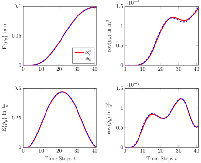
Figure 2: Mean and variance of $p_{y}$ and $\dot{p}_{y}$ (LQG). The values of $\bm{x}_{t}^{\ast}$ (resulting from $\bm{s}^{\ast}$ and $\bm{\sigma}^{\ast}$) and $\tilde{\bm{x}}_{t}$ (resulting from $\tilde{\bm{s}}$ and $\tilde{\bm{\sigma}}$) are compared. The VAF metrics are $1$ and $0.999$ in the first and second row. The corresponding values for $p_{x}$ are $1$ and $0.999$ and for $\dot{p}_{x}$ $1$ and $0.998$.

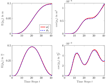
Figure 3: Mean and variance of $p_{y}$ and $\dot{p}_{y}$ (LQS). The VAF metrics are $1$ and $0.998$ in the first and $1$ and $0.996$ in the second row. The corresponding values for $p_{x}$ are $1$ and $0.999$ and for $\dot{p}_{x}$ $0.999$ and $0.965$.

In Table I the parameters $\tilde{\bm{\sigma}}$ and $\tilde{\bm{s}}$ are compared with their ground truth values $\bm{\sigma}^{\ast}$ and $\bm{s}^{\ast}$. The high accuracy of estimating the parameters of the additive noise process $\bm{\xi}_{t}$ is remarkable which is due to their strong influence on the variance of the measurable states. In addition, the cost function parameters $s_{N,1}$, $s_{N,3}$ and $s_{R,1}$ are identified correctly up to the known scaling ambiguity. Regarding the parameters $s_{N,2}$, $s_{N,4}$ and $s_{R,2}$, an additional ambiguity can be seen. In the LQG case, the 2D system is composed by two 1D systems. Hence, to describe the moments of the measurable states it is sufficient that the ratios between $s_{N,1}$, $s_{N,3}$, $s_{R,1}$ and $s_{N,2}$, $s_{N,4}$, $s_{R,2}$ are estimated correctly but not with the same reference value necessarily. Thus, changing the normalizing parameter in (21) to $s_{N,2}$ leads to $\triangle_{2}^{\bm{s}}=0$, $\triangle_{4}^{\bm{s}}=0.05$ and $\triangle_{8}^{\bm{s}}=0.01$. However, the parameters of the additive observation noise are estimated with high errors. This can be traced back to the filter equations. Since they compensate noisy observations, the underlying noise parameters cannot be determined from realizations of $\bm{x}_{t}^{\ast}$.

IV-D Results of the Linear-Quadratic Sensorimotor Case

The tuning parameters to apply Algorithm 1 to the LQS example are the same as in the subsection before. Only $\mathcal{N}_{\bm{\sigma}}=\mathcal{N}_{\bm{s}}=10$ holds and the parameter sets of the noise parameters are adapted: $\mathcal{P}_{\bm{\sigma}}=\{\{\sigma_{1},\sigma_{3}\},\{\sigma_{2},\sigma_{4}\},\{\sigma_{5},\sigma_{7},\sigma_{15}\},\{\sigma_{6},\sigma_{8},\sigma_{15}\},\{\sigma_{9},\sigma_{11},\\ \sigma_{13},\sigma_{16}\},\{\sigma_{10},\sigma_{12},\sigma_{14},\sigma_{16}\}\}$. Fig. 3 shows that our algorithm finds parameters that solve Problem 2 as well. All VAF values are $\geq 99.6\,\%$ except the one for the variance of $\dot{p}_{x}$ which still has a VAF $\geq 96.5\,\%$. The computation time was $19.9\text{\,}\mathrm{h}$. The iterative calculation of $\bm{K}_{t}$ and $\bm{L}_{t}$ at each grid point is one reason for the computational complexity. In addition, to achieve an accuracy comparable to the LQG case, the total number of grid points evaluated is greater. Table I depicts the parameter errors for the LQS example as well. As in the LQG case, the exact values of the observation noise parameters have low influence on the measurable states and thus, show high error measures. Remarkably, the scaling parameter $\sigma^{\bm{u}}$ of the control-dependent noise is estimated with high accuracy (relative error of $3\,\%$). Consequently, the control-dependent noise is the most important part of the LQS model to achieve its characteristic mean and variance curves of the measurable states. Specifically, compared to the LQG model, the peak of $\mathrm{cov}\left(p_{y}\right)$ at $t=26$ in Fig. 2 disappears in Fig. 3 and the values of $\mathrm{cov}\left(p_{y}\right)$ are lower over the complete time horizon in case of the LQS model. Furthermore, the peaks of $\mathrm{E}\left\{\dot{p}_{y}\right\}$ and $\mathrm{cov}\left(\dot{p}_{y}\right)$ appear around two steps earlier and the peaks of $\mathrm{cov}\left(\dot{p}_{y}\right)$ have nearly the same height in the LQS case.

TABLE I: Parameter errors according to (21) and (22) achieved by Algorithm 1. Values marked with ^∗ denote raw values calculated by our algorithm since the corresponding ground truth value is zero.

	LQG	LQS		LQG	LQS		LQG	LQS
$\sigma_{1}^{\bm{\xi}}$	$0^{\ast}$	$0^{\ast}$	$s_{N,1}$	$0$	$0$	$\sigma_{1}^{\bm{\omega}}$	$0.21$	$684$
$\sigma_{2}^{\bm{\xi}}$	$0^{\ast}$	$0^{\ast}$	$s_{N,2}$	$0.66$	$0$	$\sigma_{2}^{\bm{\omega}}$	$22.2$	$510$
$\sigma_{3}^{\bm{\xi}}$	$0^{\ast}$	$0^{\ast}$	$s_{N,3}$	$0.07$	$3.94$	$\sigma_{3}^{\bm{\omega}}$	$0.57$	$24.7$
$\sigma_{4}^{\bm{\xi}}$	$0^{\ast}$	$0^{\ast}$	$s_{N,4}$	$0.58$	$0.98$	$\sigma_{4}^{\bm{\omega}}$	$0.03$	$0.14$
$\sigma_{5}^{\bm{\xi}}$	$0.18^{\ast}$	$0.30^{\ast}$	$s_{N,5}$	$0.05$	$0.64$	$\sigma_{5}^{\bm{\omega}}$	$0.15$	$0.56$
$\sigma_{6}^{\bm{\xi}}$	$0.19^{\ast}$	$0.09^{\ast}$	$s_{N,6}$	$0.05$	$0.64$	$\sigma_{6}^{\bm{\omega}}$	$0.13$	$0.25$
$\sigma_{7}^{\bm{\xi}}$	$0.03$	$0.68^{\ast}$	$s_{R,1}$	$0.04$	$0.41$	$\sigma^{\bm{x}}$	-	$1.78$
$\sigma_{8}^{\bm{\xi}}$	$0.03$	$0.32^{\ast}$	$s_{R,2}$	$0.65$	$0.41$
$\sigma^{\bm{u}}$	-	$0.03$

V CONCLUSION

In this paper, we propose formal definitions of the inverse problem of the LQG and LQS control model for the first time. Solving these ISOC problems is highly relevant for the identification of the unknown parameters of these SOC models, namely weighting matrices of the cost function and covariance matrices of the noise processes, to analyze the optimality principles underlying human movements. Furthermore, we introduce a new bi-level-based algorithm, which iteratively estimates cost function and noise parameters, to solve both ISOC problems. Simulation examples show that mean and variance of system states obtained from parameters determined by our ISOC algorithm predominantly yield VAF values $\geq 99\,\%$ compared to ground truth data. Since the simulation results are very promising, we look at the application of our algorithm to real human measurement data in the next step. In addition, we investigate extensions of our approach to nonlinear systems to overcome the limitations of linear models in describing real human movements.

APPENDIX: PROOF OF LEMMA 2

Proof.

With $\bm{u}_{t}=-\bm{L}_{t}\hat{\bm{x}}_{t}$ in (11) and in the filter equation for $\hat{\bm{x}}_{t+1}$, (15) results by taking advantage of the independence between $\bm{\varepsilon}_{t}$ and $\hat{\bm{x}}_{t}$ as well as between $\bm{\epsilon}_{t}$ and $\bm{x}_{t}$. Using the same expressions for $\bm{x}_{t+1}$ and $\hat{\bm{x}}_{t+1}$ to set up the covariance, we derive

$$\left[\begin{matrix}\bm{\Omega}_{t+1}^{\bm{x}}\!\!&\bm{\Omega}_{t+1}^{\bm{x}\hat{\bm{x}}}\\ \bm{\Omega}_{t+1}^{\hat{\bm{x}}\bm{x}}\!\!&\bm{\Omega}_{t+1}^{\hat{\bm{x}}}\end{matrix}\right]=\mathrm{cov}\left(\left[\begin{matrix}\bm{x}_{t+1}\\ \hat{\bm{x}}_{t+1}\end{matrix}\right]\right)$$

$$=\bm{\mathcal{A}}_{t}\left[\begin{matrix}\bm{\Omega}_{t}^{\bm{x}}\!\!\!\!&\bm{\Omega}_{t}^{\bm{x}\hat{\bm{x}}}\\ \bm{\Omega}_{t}^{\hat{\bm{x}}\bm{x}}\!\!\!\!&\bm{\Omega}_{t}^{\hat{\bm{x}}}\end{matrix}\right]\bm{\mathcal{A}}_{t}^{\mathrm{T}}$$

$$\hphantom{=}+\mathrm{E}\left\{\left[\begin{matrix}-\sum_{i}\varepsilon_{t}^{(i)}\bm{C}_{i}\bm{L}_{t}\hat{\bm{x}}_{t}\\ \bm{K}_{t}\sum_{i}\epsilon_{t}^{(i)}\bm{D}_{i}\bm{x}_{t}\end{matrix}\right]\left[\begin{matrix}-\sum_{i}\varepsilon_{t}^{(i)}\bm{C}_{i}\bm{L}_{t}\hat{\bm{x}}_{t}\\ \bm{K}_{t}\sum_{i}\epsilon_{t}^{(i)}\bm{D}_{i}\bm{x}_{t}\end{matrix}\right]^{\mathrm{T}}\right\}$$

$$\hphantom{=}+\mathrm{E}\left\{\left[\begin{matrix}\bm{\xi}_{t}\\ \bm{\eta}_{t}+\bm{K}_{t}\bm{\omega}_{t}\end{matrix}\right]\left[\begin{matrix}\bm{\xi}_{t}\\ \bm{\eta}_{t}+\bm{K}_{t}\bm{\omega}_{t}\end{matrix}\right]^{\mathrm{T}}\right\}$$ (23)

by exploiting the following independences: $\bm{\varepsilon}_{t}$ to $\hat{\bm{x}}_{t}$; $\bm{\epsilon}_{t}$ to $\bm{x}_{t}$; $\bm{\xi}_{t}$ to $\bm{x}_{t}$, $\hat{\bm{x}}_{t}$, $\bm{\varepsilon}_{t}$ and $\bm{\epsilon}_{t}$; $\bm{\eta}_{t}$ to $\bm{x}_{t}$, $\hat{\bm{x}}_{t}$, $\bm{\varepsilon}_{t}$ and $\bm{\epsilon}_{t}$; $\bm{\omega}_{t}$ to $\bm{x}_{t}$, $\hat{\bm{x}}_{t}$, $\bm{\varepsilon}_{t}$ and $\bm{\epsilon}_{t}$. From the independence of $\bm{\xi}_{t}$ to $\bm{\eta}_{t}$ and $\bm{\omega}_{t}$

$$\left[\begin{matrix}\bm{\Omega}^{\bm{\xi}}\!\!&\bm{0}\\ \bm{0}\!\!&\bm{\Omega}^{\bm{\eta}}+\bm{K}_{t}\bm{\Omega}^{\bm{\omega}}\bm{K}_{t}^{\mathrm{T}}\end{matrix}\right]$$ (24)

follows for the third summand in (23). Each element of the matrix of the second summand in (23) can be simplified by considering the independence of $\bm{\varepsilon}_{t}$ and $\bm{\epsilon}_{t}$ to $\bm{x}_{t}$ and $\hat{\bm{x}}_{t}$ as well as $\mathrm{E}\left\{\varepsilon_{t}^{(i)}\varepsilon_{t}^{(j)}\right\}=\mathrm{E}\left\{\epsilon_{t}^{(i)}\epsilon_{t}^{(j)}\right\}=\delta_{ij}$ ($\delta_{ij}=1$ for $i=j$, $\delta_{ij}=0$ for $i\neq j$) and $\mathrm{E}\left\{\varepsilon_{t}^{(i)}\epsilon_{t}^{(j)}\right\}=0$ ($\forall i,j$):

$$\mathrm{E}\left\{\sum_{i}\varepsilon_{t}^{(i)}\bm{C}_{i}\bm{L}_{t}\hat{\bm{x}}_{t}\hat{\bm{x}}_{t}^{\mathrm{T}}\bm{L}_{t}^{\mathrm{T}}\sum_{j}\bm{C}_{j}^{\mathrm{T}}\varepsilon_{t}^{(j)}\right\}$$

$$=\sum_{i}\bm{C}_{i}\bm{L}_{t}\mathrm{E}\left\{\hat{\bm{x}}_{t}\hat{\bm{x}}_{t}^{\mathrm{T}}\right\}\bm{L}_{t}^{\mathrm{T}}\bm{C}_{i}^{\mathrm{T}}$$ (25)

$$\mathrm{E}\left\{-\sum_{i}\varepsilon_{t}^{(i)}\bm{C}_{i}\bm{L}_{t}\hat{\bm{x}}_{t}\bm{x}_{t}^{\mathrm{T}}\sum_{j}\bm{D}_{j}^{\mathrm{T}}\epsilon_{t}^{(j)}\bm{K}_{t}^{\mathrm{T}}\right\}=\bm{0}$$ (26)

$$\mathrm{E}\left\{-\bm{K}_{t}\sum_{i}\epsilon_{t}^{(i)}\bm{D}_{i}\bm{x}_{t}\hat{\bm{x}}_{t}^{\mathrm{T}}\bm{L}_{t}\sum_{j}\bm{C}_{j}^{\mathrm{T}}\varepsilon_{t}^{(j)}\right\}=\bm{0}$$ (27)

$$\mathrm{E}\left\{\bm{K}_{t}\sum_{i}\epsilon_{t}^{(i)}\bm{D}_{i}\bm{x}_{t}\bm{x}_{t}^{\mathrm{T}}\sum_{j}\bm{D}_{j}^{\mathrm{T}}\epsilon_{t}^{(j)}\bm{K}_{t}^{\mathrm{T}}\right\}$$

$$=\sum_{i}\bm{K}_{t}\bm{D}_{i}\mathrm{E}\left\{\bm{x}_{t}\bm{x}_{t}^{\mathrm{T}}\right\}\bm{D}_{i}^{\mathrm{T}}\bm{K}_{t}^{\mathrm{T}}.$$ (28)

With $\mathrm{E}\left\{\hat{\bm{x}}_{t}\hat{\bm{x}}_{t}^{\mathrm{T}}\right\}=\bm{\Omega}_{t}^{\hat{\bm{x}}}+\mathrm{E}\left\{\hat{\bm{x}}_{t}\right\}\mathrm{E}\left\{\hat{\bm{x}}_{t}\right\}^{\mathrm{T}}$ in (25) and $\mathrm{E}\left\{\bm{x}_{t}\bm{x}_{t}^{\mathrm{T}}\right\}=\bm{\Omega}_{t}^{\bm{x}}+\mathrm{E}\left\{\bm{x}_{t}\right\}\mathrm{E}\left\{\bm{x}_{t}\right\}^{\mathrm{T}}$ in (28), (23) reduces to (16). The initial values follow analogously to the proof of Lemma 1.

References

• [1] J. P. Gallivan, C. S. Chapman, D. M. Wolpert, and J. R. Flanagan, “Decision-making in sensorimotor control,” Nat. Rev. Neurosci., vol. 19, no. 9, pp. 519–534, 2018.
• [2] E. Todorov and M. I. Jordan, “Optimal feedback control as a theory of motor coordination,” Nat. Neurosci., vol. 5, no. 11, pp. 1226–1235, 2002.
• [3] E. Todorov, “Optimality principles in sensorimotor control,” Nat. Neurosci., vol. 7, no. 9, pp. 907–915, 2004.
• [4] ——, “Stochastic optimal control and estimation methods adapted to the noise characteristics of the sensorimotor system,” Neural Comput., vol. 17, pp. 1084–1108, 2005.
• [5] B. Berret, A. Conessa, N. Schweighofer, and E. Burdet, “Stochastic optimal feedforward-feedback control determines timing and variability of arm movements with or without vision,” PLoS Comput. Biol., vol. 17, no. 6, 2021.
• [6] M. C. Priess, J. Choi, and C. Radcliffe, “The inverse problem of continuous-time linear quadratic gaussian control with application to biological systems analysis,” ASME 2014 Dynamic Systems and Control Conference, 2014.
• [7] X. Chen and B. D. Ziebart, “Predictive inverse optimal control for linear-quadratic-gaussian systems,” 18th Int. Conf. on Artificial Intelligence and Statistics, 2015.
• [8] W. Li, E. Todorov, and D. Liu, “Inverse optimality design for biological movement systems,” IFAC Proc. Volumes, vol. 44, no. 1, pp. 9662–9667, 2011.
• [9] M. Schultheis, D. Straub, and C. A. Rothkopf, “Inverse optimal control adapted to the noise characteristics of the human sensorimotor system,” 35th Conference on Neural Information Processing Systems (NeurIPS 2021), 2021.
• [10] S. Kolekar, W. Mugge, and D. Abbink, “Modeling intradriver steering variability based on sensorimotor control theories,” IEEE Trans. Hum.-Mach. Syst., vol. 48, no. 3, pp. 291–303, 2018.
• [11] B. Berret, E. Chiovetto, F. Nori, and T. Pozzo, “Evidence for composite cost functions in arm movement planning: an inverse optimal control approach,” PLoS Comput. Biol., vol. 7, no. 10, 2011.
• [12] S. Albrecht, M. Leibold, and M. Ulbrich, “A bilevel optimization approach to obtain optimal cost functions for human arm movements,” Numer. Algebra, Control. Optim., vol. 2, no. 1, pp. 105–127, 2012.
• [13] O. S. Oguz, Z. Zhou, S. Glasauer, and D. Wollherr, “An inverse optimal control approach to explain human arm reaching control based on multiple internal models,” Sci. Rep., vol. 8, no. 1, 2018.
• [14] J. F.-S. Lin, V. Bonnet, A. M. Panchea, N. Ramdani, G. Venture, and D. Kulic, “Human motion segmentation using cost weights recovered from inverse optimal control,” Int. Conf. on Humanoid Robots (Humanoids), 2016.
• [15] A. M. Panchea, N. Ramdani, V. Bonnet, and P. Fraisse, “Human arm motion analysis based on the inverse optimization approach,” 7th IEEE Int. Conf. on Biomedical Robotics and Biomechatronics (BioRob), 2018.
• [16] K. Westermann, J. F.-S. Lin, and D. Kulić, “Inverse optimal control with time-varying objectives: application to human jumping movement analysis,” Sci. Rep., vol. 10, no. 1, 2020.
• [17] W. Jin, D. Kulic, J. F.-S. Lin, S. Mou, and S. Hirche, “Inverse optimal control for multiphase cost functions,” IEEE Trans. Rob., vol. 35, no. 6, pp. 1387–1398, 2019.
• [18] T. Flash and N. Hogan, “The coordination of arm movements: an experimentally confirmed mathematical model,” J. Neurosci., vol. 5, no. 7, pp. 1688–1703, 1985.
• [19] Y. Uno, M. Kawato, and R. Suzuki, “Formation and control of optimal trajectory in human multijoint arm movement,” Biol. Cybern., vol. 61, pp. 89–101, 1989.
• [20] K. J. Aström, Introduction to Stochastic Control Theory.   New York: Academic Press, Inc., 1970.
• [21] T. L. Molloy, J. Inga, M. Flad, J. J. Ford, T. Perez, and S. Hohmann, “Inverse open-loop noncooperative differential games and inverse optimal control,” IEEE Trans. Autom. Control, vol. 65, no. 2, pp. 897–904, 2020.
• [22] K. Mombaur, A. Truong, and J.-P. Laumond, “From human to humanoid locomotion—an inverse optimal control approach,” Auton. Robots, vol. 28, no. 3, pp. 369–383, 2010.
• [23] J. C. Bezdek and R. J. Hathaway, “Some notes on alternating optimization,” AFSS International Conference on Fuzzy Systems, 2002.