Joint BS-RIS-User Association and Beamforming Design for RIS-assisted Cellular Networks

Abstract

Reconfigurable intelligent surface (RIS) is a revolutionary technology for sixth-generation (6G) networks owing to its ability to manipulate wireless environments. As a frequency-selective device, RIS can only effectively shape the propagation of signals within a certain frequency band. Due to this frequency-selective property, the deployment of RIS in cellular networks will introduce a complicated base station (BS)-RIS-user association issue since adjacent BSs operate at different frequency bands. In this paper, with the consideration of the frequency-selective characteristics of RIS, we aim to jointly optimize BS-RIS-user association, active beamforming at BSs, and passive beamforming of RIS to maximize the sum-rate of a RIS-assisted cellular network. We first leverage $l_{0}$-norm to efficiently integrate BS-RIS-user association with active and passive beamforming. Then, we adopt fractional programming (FP) and block coordinate descent (BCD) methods to deal with logarithmic and fractional parts and decouple the joint association and beamforming design problem into several sub-problems. Efficient algorithms which combine $l_{0}$-norm approximation, majorization-minimization (MM), and alternating direction method of multipliers (ADMM) are developed to alternately solve the sub-problems. Extensive simulation results illustrate the importance of BS-RIS-user association optimization in RIS-assisted cellular networks and verify the effectiveness of the proposed joint association and beamforming design algorithm.

I Introduction

Recently, with the rapid deployment of commercial fifth-generation (5G) wireless networks worldwide, researchers shift their interests to future sixth-generation (6G) systems, which require higher data rate and network capacity. However, the existing technologies in 5G, e.g., massive multiple-input multiple-output (MIMO), millimeter wave (mmWave) communications, and ultra-dense heterogeneous network have reached their inherent limitations on transmission rate, spectrum/energy efficiency, etc. Thereby, innovative technologies are needed to achieve radical changes.

In conventional networks, the wireless propagation environment is regarded as a randomly varied uncontrollable factor, which cannot be optimized in the network design. Recently, an innovative reconfigurable intelligent surface (RIS) technology is introduced to radically change this conventional perception. RIS is deemed as a revolutionary and promising technology for 6G because of its ability to reconfigure the wireless propagation environment [1]-[4]. To be specific, RIS is a meta-surface consists of a large number of low-cost passive reflecting elements. Each element can be independently controlled to collaboratively achieve passive reflection beamforming by adjusting the amplitude/phase-shift of incident signals. Owing to the superior ability of shaping wireless propagation environment, the deployment of RIS can provide new degrees of freedom (DoFs) for the design of wireless networks, which can significantly improve the performance of networks.

Benefiting from the simple and passive hardware architecture, RIS features low energy consumption, low hardware cost, and easy installation, etc. These appealing advantages stimulate many research efforts of designing RIS-assisted wireless communication systems using different metrics, including maximizing spectral efficiency [5], maximizing energy efficiency [6], [7], maximizing sum-rate of all users [8]-[10], maximizing received power [11], and minimizing transmit power [12]-[14], etc. In addition, due to passive and massive RIS reflecting elements, channel state information (CSI) acquisition is challenging, which has triggered the research on efficient channel estimation for RIS-assisted wireless systems [15]-[21]. Moreover, RIS is also applied in combination with other emerging technologies, such as non-orthogonal multiple-access (NOMA) [22], [23], simultaneous wireless information and power transfer (SWIPT) [24], [25], symbol-level precoding (SLP) [26], [27], holographic MIMO (HMIMO) [28], integrated sensing and communications (ISAC) [29]-[32], etc.

Most existing works on RIS-assisted systems consider relatively simple scenarios with only one transmitter or base station (BS). In order to accelerate the deployment of RIS in realistic cellular networks, the design of RIS in multi-cell systems is also a worth studying problem. Moreover, two special and crucial issues are needed to be considered for the RIS-assisted cellular network. Firstly, some existing works illustrated the frequency-selective property of RIS. By considering the hardware complexity and cost in practical implementations, this property can be approximately modeled as: Each element of RIS can only effectively provide tunable phase-shift for signals within a certain frequency band, while generates almost fixed phase-shift for signals at other frequency bands [33]-[36]. Notice that the performance loss caused by this simplified RIS model is verified to be negligible [36]. Considering that the adjacent BSs usually operate at different frequency bands in the cellular network, the practical RIS with this frequency-selective property can only optimize its phase-shifts to effectively assist one BS operating at a certain frequency band, while its phase-shifts are almost fixed for signals from other BSs. This fact means that the BS-RIS association problem deserves to be carefully studied in the RIS-assisted multi-cell system and effective association algorithms need to be developed for this new BS-RIS association problem. Secondly, the deployment of RIS introduces a different and more complicated BS-user association problem than conventional multi-cell systems, because the BS-user link relies not only on the direct channels, but also on the BS-RIS-user cascaded channels. Moreover, since RIS can reflect the signals from all associated/un-associated BSs, the BS-user association in all cells will be affected. This fact reveals that the traditional user association algorithms cannot be directly adopted in RIS-assisted systems, which inspires us to investigate new BS-user association algorithms.

Some researchers have noticed the impact of deploying RIS on the user association as well as the RIS association in cellular networks and started to investigate these BS-user [37]-[39], BS-RIS [40], RIS-user [41], [42], or BS-RIS-user [43], [44] association problems in RIS-assisted systems. In [37], the authors proposed a load balancing BS-user association scheme for multi-RIS assisted multi-cell system, in which each BS can be assisted by one RIS. In [38], a BS-user association and passive beamforming optimization problem based on statistical CSI was investigated for a multi-BS multi-RIS heterogeneous network. The authors in [39] presented a joint power allocation and BS-user association design problem for mmWave systems. However, the authors of these works [37]-[39] assumed that the BS-RIS association is fixed, which is not realistic. Moreover, they ignored that the RIS can reflect the signals of all BSs rather than only the associated BS. The authors in [40] focused on the BS-RIS association and beamforming design problem and proposed a multi-agent deep reinforcement learning-based association scheme. The authors in [41] considered a RIS-user association and cascaded channel estimation problem, while the authors in [42] presented the RIS-user association problem with fixed BS-user association. The authors in [43] aimed to maximize the utility of users by optimizing the BS-RIS-user association and passive beamforming in a multi-BS multi-RIS narrow-band system. Nevertheless, the authors in [43] did not take the active beamforming optimization into consideration. Furthermore, they only designed the passive beamforming by aligning the angles of direct and cascade channels when the RIS is associated with one BS, which ignores the impact of the reflecting signals from other BSs. In [44], a BS-RIS-user association and beamforming design problem was investigated for a cellular network, in which the power allocation of users in each cell is not considered.

These existing works reviewed above only investigate part of joint BS-RIS-user association, active beamforming, and passive beamforming design, but ignore that the BS-RIS-user association and active/passive beamforming optimization problems are tightly interrelated and inseparable. More importantly, the frequency-selective property of RIS has not been considered in most of the existing literatures. These facts mean that most of the existing association algorithms cannot be directly utilized in the joint BS-RIS-user association and beamforming design for practical RIS-assisted systems. Thus, the association and beamforming design in practical RIS-assisted systems is worth to be investigated, which is more practical, comprehensive, and realistic compared with the existing works. Motivated by above discussion, in this paper we consider a practical RIS-assisted multi-cell wireless network and focus on the BS-RIS-user association as well as the active and passive beamforming optimization. Our main contributions are summarized as follows:

• Different from most of existing works which only consider part of the BS-RIS-user association problem with an ideal RIS model, a more comprehensive and realistic practical RIS-assisted multi-cell network is modeled, in which we concern about the joint design of BS-RIS-user association, the active beamforming of BSs, and the passive beamforming of RIS. It is worth mentioning that we adopt the practical RIS reflecting model which describes the frequency-selective characteristics of RIS [33]-[36]. The sum-rate maximization problem is then formulated, which aims to maximize the sum-rate of all users in the cellular network subject to the power budgets of BSs, the association constraints, and the restrict of RIS elements.

• To facilitate the joint association and beamforming design, we utilize $l_{0}$-norm to combine the active beamforming with BS-user association and integrate the passive beamforming with BS-RIS association. Then, in order to solve the non-convex non-smooth joint association and beamforming optimization problem, we first adopt the fractional programming (FP) and block coordinate descent (BCD) method to deal with logarithmic and fractional parts, and then decouple the problem into several sub-problems. Efficient algorithms which combine $l_{0}$-norm approximation, majorization-minimization (MM), and alternating direction method of multipliers (ADMM) are developed to alternately solve the sub-problems.

• Finally, extensive simulation results are provided to verify the importance of the joint association and beamforming design as well as the effectiveness of our proposed algorithm. To be specific, the proposed joint association and beamforming design algorithm facilitates load balancing between BSs, which is beneficial to the utilization of resources. Moreover, our proposed algorithm has significant performance improvement compared with benchmark algorithms, which demonstrates the advancement of joint BS-RIS-user association design.

Notations: Boldface lower-case, boldface upper-case, and Italic letters indicate column vectors, matrices, and scalars, respectively. $\mathbb{C}$ and $\mathbb{R}$ denote the sets of complex and real numbers, respectively. $\jmath$ presents the imaginary unit. For a complex valued vector $\boldsymbol{a}$, $\|\boldsymbol{a}\|_{0}$ and $\|\boldsymbol{a}\|_{2}$ denote its $l_{0}$-norm and $l_{2}$-norm, respectively. $\mathbf{A}^{T}$ and $\mathbf{A}^{H}$ denotes the transpose and conjugate transpose for matrix $\mathbf{A}$, respectively. $\mathbb{E}\{\cdot\}$ and $\mathfrak{Re}\{\cdot\}$ indicate statistical expectation and the real part of a complex number, respectively. $\mathbf{I}_{M}$ presents an $M\times M$ identity matrix. $\oslash$ denotes the element-wise division.

II System Model and Problem Formulation

II-A System Model

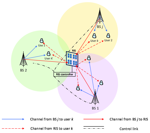
Figure 1: RIS-assisted multi-cell MU-MISO wireless communication network.

We consider a RIS-assisted multi-cell wireless network as shown in Fig. 1, where $K$ single-antenna users are served by $J$ BSs operating at different frequency bands. Each BS is equipped with $M$ antennas and can simultaneously transmit independent data streams to a maximum of $K$ users. Furthermore, a RIS, which consists of $N$ reflecting elements, is deployed to assist the communications between BSs and their associated users. Thus, each cell can be deemed as a RIS-assisted multi-user multiple-input single-output (MU-MISO) system. For brevity, let $\mathcal{J}=\{1,2,...,J\}$, $\mathcal{K}=\{1,2,...,K\}$, and $\mathcal{N}=\{1,2,...,N\}$ denote the sets of BSs, users, and RIS reflecting elements, respectively. In addition, we assume that the RIS is controlled by BSs via dedicated wireless or wired links. Furthermore, for the channel estimation in RIS-assisted systems, many effective and efficient frameworks/algorithms have been proposed, which can achieve accurate channel estimation with low pilot overhead [15]-[21]. Thus, we also assume that the CSI of all channels are perfectly estimated and known by BSs.

Recent works illustrate that the reflecting elements of a practical RIS can be approximately considered only providing tunable phase-shifts for the signals within a certain frequency band (the frequency band can be modified by adjusting the capacitance of RIS elements), and having almost fixed ($0$ or $2\pi$) phase-shifts for the signals at other frequency bands [33]-[36]. Meanwhile, this simplified practical model can significantly reduce the computational complexity for the RIS passive beamforming design compared with the practical RIS which is modeled by microwave theory, while the performance loss caused by the approximation is verified to be negligible [36]. This important frequency-selective feature indicates that the deployed RIS can effectively change the propagation of signals for only one BS, since adjacent BSs operate at different frequency bands. In other words, the RIS can only effectively serve one BS by adaptively manipulating the wireless propagation between this BS and its users. Thus, BS-RIS association with the consideration of the frequency-selective property of RIS is a new but crucial problem in the RIS-assisted network. To efficiently express the BS-RIS association as well as the passive beamforming of RIS, we first assume that the phase-shifts of RIS are fixed as $0$ for the signals at other un-associated BSs’ operating frequency bands, since phase-shifts $0$ or $2\pi$ will generate the same reflecting coefficients. By defining the phase-shifts of RIS for BS-$j$ as $\boldsymbol{\theta}_{j}\triangleq[\theta_{j,1},\theta_{j,2},...,\theta_{j,N}]^{T}$, the BS-RIS association and passive beamforming can be combined. Specifically, $\boldsymbol{\theta}_{j}=\mathbf{0}_{N}$ indicates that BS-$j$ is not assisted by RIS, i.e., the phase-shifts are not tunable and fixed as zeros; otherwise, $\boldsymbol{\theta}_{j}\neq\mathbf{0}_{N}$ represents that RIS will assist BS-$j$ by adaptively tuning the phase-shifts for the signals at the frequency band of BS-$j$. Then, the passive beamforming matrix of RIS for BS-$j$ can be represented by $\boldsymbol{\Phi}_{j}\triangleq\operatorname{diag}(\boldsymbol{\varphi}_{j})$, where $\boldsymbol{\varphi}_{j}\triangleq e^{\jmath\boldsymbol{\theta}_{j}}=[e^{\jmath\theta_{j,1}},e^{\jmath\theta_{j,2}},...,e^{\jmath\theta_{j,N}}]^{T}$.

According to the frequency-selective characteristics of RIS, it can only assist at most one BS and serve its associated users in the cellular system. This feature in BS-RIS association can be easily expressed as the constraint $\big{\|}[\left\|\boldsymbol{\theta}_{1}\right\|_{2}^{2},...,\left\|\boldsymbol{\theta}_{J}\right\|_{2}^{2}]\big{\|}_{0}=\sum_{j\in\mathcal{J}}\big{\|}\left\|\boldsymbol{\theta}_{j}\right\|_{2}^{2}\big{\|}_{0}=1$ by utilizing $l_{0}$-norm, which represents the number of non-zero elements in vector $[\left\|\boldsymbol{\theta}_{1}\right\|_{2}^{2},...,\left\|\boldsymbol{\theta}_{J}\right\|_{2}^{2}]^{T}$. In order to convert the problem into a more common form, we prefer to use the reflecting coefficient $\boldsymbol{\varphi}_{j}$ instead of the angle $\boldsymbol{\theta}_{j}$ in this constraint. Thus, based on the definition $\boldsymbol{\varphi}_{j}\triangleq e^{\jmath\boldsymbol{\theta}_{j}}$, the BS-RIS association constraint can be reformulated as

$$\sum_{j\in\mathcal{J}}\big{\|}\|\boldsymbol{\theta}_{j}\|_{2}^{2}\big{\|}_{0}\overset{\text{(a)}}{=} \sum_{j\in\mathcal{J}}\left\|\left\|-\jmath\ln(\boldsymbol{\varphi}_{j})\right\|_{2}^{2}\right\|_{0}$$ (1)

$$\overset{\text{(b)}}{=} \sum_{j\in\mathcal{J}}\left\|\left\|\ln(\boldsymbol{\varphi}_{j})\right\|_{2}^{2}\right\|_{0}=1,$$

where $\ln(\boldsymbol{\varphi}_{j})$ represents an element-wise natural logarithmic operation. The equality (a) holds according to the definition of complex logarithmic function, i.e., $a=\log(b)=\log|b|+\jmath(\arg(b)+2k\pi),~{}k=0,\pm 1,\pm 2,...$, in which $a$ and $b$ are complex numbers. Then, with the unit modulus of $\varphi_{j,n}$, we can obtain the phase-shift of $\varphi_{j,n}$ by logarithmic operations. Notice that we only concern about the principal value $\boldsymbol{\theta}_{j}=-\jmath\ln(\boldsymbol{\varphi}_{j})$, which lies in the definition domain $\left[-\pi,\pi\right)$. Equality (b) holds since $\jmath^{2}=-1$.

On the other hand, the association between BSs and users is also significantly affected by the deployment of RIS due to additional reconfigurable BS-RIS-user cascaded channel. Considering that the conventional BS-user association algorithms cannot be directly applied for the RIS-assisted network, we should carefully elaborate on the BS-user association problem for the considered system. Similar to the integration of BS-RIS association and passive beamforming, we combine the BS-user association with the active beamforming by utilizing $l_{0}$-norm. Specifically, we first define $\mathbf{w}_{j,k}\in\mathbb{C}^{M\times 1}$ as the beamforming vector at BS-$j$ for user-$k$. When user-$k$ is not served by BS-$j$, active beamforming $\mathbf{w}_{j,k}=\mathbf{0}_{M}$; otherwise, if user-$k$ is associated with BS-$j$, $\mathbf{w}_{j,k}\neq\mathbf{0}_{M}$ and can be optimized. Since we assume that each user is served by only one BS, the BS-user association can be expressed as the constraint $\big{\|}[\left\|\mathbf{w}_{1,k}\right\|_{2}^{2},...,\left\|\mathbf{w}_{J,k}\right\|_{2}^{2}]\big{\|}_{0}=\sum_{j\in\mathcal{J}}\big{\|}\left\|\mathbf{w}_{j,k}\right\|_{2}^{2}\big{\|}_{0}=1,~{}\forall k$.

Denote $s_{j,k}$ as the symbol transmitted from BS-$j$ to user-$k$, which satisfies $\mathbb{E}\{s_{j,k}s_{j,k}^{*}\}=1$ and $\mathbb{E}\{s_{j,k}s_{j,i}^{*}\}=0,~{}\forall i\neq k$. We should emphasize that the symbol $s_{j,k}$ is meaningful only when BS-$j$ is associated to user-$k$. Thus, by denoting $\mathbf{h}_{\text{d},j,k}\in\mathbb{C}^{M\times 1}$, $\mathbf{G}_{j}\in\mathbb{C}^{N\times M}$, and $\mathbf{h}_{\text{r},k}\in\mathbb{C}^{N\times 1}$, $\forall j,~{}\forall k$ as the channels from BS-$j$ to user-$k$, from BS-$j$ to RIS, and from RIS to user-$k$, respectively, the received signal of user-$k$ from the BS-$j$ can be written as

$$y_{j,k}=\left\{\begin{array}[]{ll}\sum\limits_{i\in\mathcal{K}}\widetilde{\mathbf{h}}_{j,k}^{H}\mathbf{w}_{j,i}s_{j,i}+n_{k},&\text{BS-}j\text{ serves user-}k,\\ 0,&\text{otherwise},\end{array}\right.$$ (2)

in which we define $\widetilde{\mathbf{h}}_{j,k}^{H}\triangleq\mathbf{h}_{\text{d},j,k}^{H}+\mathbf{h}_{\text{r},k}^{H}\boldsymbol{\Phi}_{j}\mathbf{G}_{j}$ as the equivalent compound channel from BS-$j$ to user-$k$ for brevity. $n_{k}\sim\mathcal{CN}(0,\sigma^{2}_{k})$ is complex additive white Gaussian noise with variance $\sigma^{2}_{k}$ and zero mean.

Then, the signal-to-interference-plus-noise ratio (SINR) of user-$k$ can be represented as

$$\mathrm{SINR}_{j,k}= \frac{|\widetilde{\mathbf{h}}_{j,k}^{H}\mathbf{w}_{j,k}|^{2}}{\sum\limits_{i\in\mathcal{K},i\neq k}|\widetilde{\mathbf{h}}_{j,k}^{H}\mathbf{w}_{j,i}|^{2}+\sigma^{2}_{k}},~{}\forall j,~{}\forall k.$$ (3)

Hence, the achievable rate of user-$k$ can be calculated by

$$R_{j,k}=\log_{2}\left(1+\mathrm{SINR}_{j,k}\right),~{}\forall j,~{}\forall k.$$ (4)

Similar to the transmitted symbol $s_{j,k}$, $\mathrm{SINR}_{j,k}$ and $R_{j,k}$ have meaningful values only when user-$k$ is served by BS-$j$; otherwise, they are meaningless and their values are all zeros.

II-B Problem Formulation

We aim to maximize the achievable sum-rate by jointly optimizing the active beamforming $\mathbf{w}_{j,k}$ and passive beamforming $\boldsymbol{\varphi}_{j}$, which also indicate BS-user association and BS-RIS association, respectively. Thus, the sum-rate maximization problem is formulated as

$$\mathop{\max}\limits_{\begin{subarray}{c}\mathbf{w}_{j,k},\boldsymbol{\varphi}_{j}\\ \forall j\in\mathcal{J},\forall k\in\mathcal{K}\end{subarray}}\; \sum_{j\in\mathcal{J}}\sum_{k\in\mathcal{K}}R_{j,k}$$ (5a)

s.t. $$\sum_{k\in\mathcal{K}}\left\|\mathbf{w}_{j,k}\right\|_{2}^{2}\leq P_{j},~{}\forall j,$$ (5b)

$$\sum_{j\in\mathcal{J}}\left\|\left\|\mathbf{w}_{j,k}\right\|_{2}^{2}\right\|_{0}=1,~{}\forall k,$$ (5c)

$$|\varphi_{j,n}|=1,~{}\forall j,~{}\forall n,$$ (5d)

$$\sum_{j\in\mathcal{J}}\left\|\left\|\ln(\boldsymbol{\varphi}_{j})\right\|_{2}^{2}\right\|_{0}=1,$$ (5e)

where $P_{j}$ is the maximum transmit power of BS-$j$. Constraint (5c) indicates that each user can only be served by one BS, and constraint (5e) implies that RIS can serve only one BS.

The non-smooth non-convex problem (5) is difficult to solve because of the non-convex objective function (5a), non-smooth non-convex constraints (5c), (5e), unit-modulus constraint (5d), and highly-coupled variables. In order to tackle these difficulties, we propose an FP-MM-ADMM based joint association and beamforming design algorithm.

III Association and Beamforming Design

In this section, we present the proposed FP-MM-ADMM based joint association and beamforming design algorithm. To be specific, we utilize the FP method to convert the logarithmic and fractional objective function into a more tractable form. Then, we adopt the BCD method to decompose the coupled variables and alternately solve the three resulting sub-problems, i.e., 1) the update of auxiliary variables, 2) the joint BS-user association and active beamforming optimization problem, and 3) the joint BS-RIS association and passive beamforming optimization problem.

III-A Objective Function Transformation

In this subsection, we attempt to deal with the non-convex objective function (5a) by FP method proposed in [45]. We first use the Lagrangian dual transform to handle the logarithmic form. By introducing the dual variable $\boldsymbol{\tau}\triangleq[\tau_{1,1},...,\tau_{j,k},...,\tau_{J,K}]^{T}$, the objective function (5a) is equivalently written as

$$\sum_{j\in\mathcal{J}} \sum_{k\in\mathcal{K}}\log_{2}\left(1+\tau_{j,k}\right)-\frac{1}{\ln 2}\sum_{j\in\mathcal{J}}\sum_{k\in\mathcal{K}}\tau_{j,k}$$ (6)

$$+\frac{1}{\ln 2}\sum_{j\in\mathcal{J}}\sum_{k\in\mathcal{K}}\frac{\left(1+\tau_{j,k}\right)|\widetilde{\mathbf{h}}_{j,k}^{H}\mathbf{w}_{j,k}|^{2}}{\sum\limits_{i\in\mathcal{K}}|\widetilde{\mathbf{h}}_{j,k}^{H}\mathbf{w}_{j,i}|^{2}+\sigma^{2}_{k}}.$$

Then, to deal with the fractional part, we adopt the quadratic transform by further introducing another auxiliary variable $\mathbf{q}\triangleq[q_{1,1},...,q_{j,k},...,q_{J,K}]^{T}$, which is used to decouple the numerators and denominators. By denoting $\mathbf{w}\triangleq[\mathbf{w}_{1,1}^{H},...,\mathbf{w}_{j,k}^{H},...,\mathbf{w}_{J,K}^{H}]^{H}$ and $\boldsymbol{\varphi}\triangleq[\boldsymbol{\varphi}_{1}^{H},...,\boldsymbol{\varphi}_{J}^{H}]^{H}$, the objective function (6) can be further converted into (7) shown at the top of next page.

$$f(\boldsymbol{\tau},\mathbf{q},\mathbf{w},\boldsymbol{\varphi})\triangleq \sum_{j\in\mathcal{J}}\sum_{k\in\mathcal{K}}\log_{2}\left(1+\tau_{j,k}\right)-\frac{1}{\ln 2}\sum_{j\in\mathcal{J}}\sum_{k\in\mathcal{K}}\tau_{j,k}$$ (7)

$$+\frac{1}{\ln 2}\bigg{(}\sum_{j\in\mathcal{J}}\sum_{k\in\mathcal{K}}2\sqrt{1+\tau_{j,k}}\mathfrak{Re}\{q_{j,k}^{*}\widetilde{\mathbf{h}}_{j,k}^{H}\mathbf{w}_{j,k}\}-\sum_{j\in\mathcal{J}}\sum_{k\in\mathcal{K}}\left|q_{j,k}\right|^{2}\Big{(}\sum_{i\in\mathcal{K}}\left|\widetilde{\mathbf{h}}_{j,k}^{H}\mathbf{w}_{j,i}\right|^{2}+\sigma^{2}_{k}\Big{)}\bigg{)}.$$

which is concave with respect to each variable. To handle the highly coupled optimization variables $\boldsymbol{\tau}$, $\mathbf{q}$, $\mathbf{w}$, and $\boldsymbol{\varphi}$ in this objective function, we adopt the BCD method to alternately update them as follows.

III-B Update Auxiliary Variables $\boldsymbol{\tau}$ and $\mathbf{q}$

With fixed $\mathbf{q}$, $\mathbf{w}$, and $\boldsymbol{\varphi}$, it is obvious that the objective function (7) is concave with respect to $\tau_{j,k}$. Thus, we can easily obtain the optimal solution of $\tau_{j,k}$ by setting $\partial f/\partial\tau_{j,k}=0$ with respect to each $j\in\mathcal{J},~{}k\in\mathcal{K}$. The optimal solution of $\tau_{j,k}$ is then calculated as

$$\tau_{j,k}^{\star}=\frac{|\widetilde{\mathbf{h}}_{j,k}^{H}\mathbf{w}_{j,k}|^{2}}{\sum\limits_{i\in\mathcal{K},i\neq k}|\widetilde{\mathbf{h}}_{j,k}^{H}\mathbf{w}_{j,i}|^{2}+\sigma^{2}_{k}},~{}\forall j,~{}\forall k.$$ (8)

Similarly, the optimal solution of $q_{j,k}$ can be obtained by setting $\partial f/\partial q_{j,k}=0$ as

$$q_{j,k}^{\star}=\frac{\sqrt{1+\tau_{j,k}}\hskip 5.69046pt\widetilde{\mathbf{h}}_{j,k}^{H}\mathbf{w}_{j,k}}{\sum\limits_{i\in\mathcal{K}}\big{|}\widetilde{\mathbf{h}}_{j,k}^{H}\mathbf{w}_{j,i}\big{|}^{2}+\sigma^{2}_{k}},~{}\forall j,~{}\forall k.$$ (9)

III-C Update Active Beamforming $\mathbf{w}$

In this subsection, we introduce an MM based algorithm to optimize the active beamforming. Since the BS-user association can be represented by the active beamforming, we can easily obtain the association results based on the resulting active beamforming. With fixed $\boldsymbol{\tau}$, $\mathbf{q}$, and $\boldsymbol{\varphi}$, the active beamforming optimization problem is reduced to

$$\mathop{\max}\limits_{\begin{subarray}{c}\mathbf{w}\end{subarray}}\; \sum_{j\in\mathcal{J}}\sum_{k\in\mathcal{K}}(-\mathbf{w}_{j,k}^{H}\boldsymbol{\Upsilon}_{j}\mathbf{w}_{j,k}+\mathfrak{Re}\{\boldsymbol{\alpha}_{j,k}^{H}\mathbf{w}_{j,k}\}-\varsigma_{j,k})$$ (10a)

s.t. $$\sum_{k\in\mathcal{K}}\left\|\mathbf{w}_{j,k}\right\|_{2}^{2}\leq P_{j},~{}\forall j,$$ (10b)

$$\sum_{j\in\mathcal{J}}\left\|\left\|\mathbf{w}_{j,k}\right\|_{2}^{2}\right\|_{0}=1,~{}\forall k,$$ (10c)

in which we define

$$\boldsymbol{\Upsilon}_{j} \triangleq\sum_{k\in\mathcal{K}}|q_{j,k}|^{2}\widetilde{\mathbf{h}}_{j,k}\widetilde{\mathbf{h}}_{j,k}^{H},$$ (11a)

$$\boldsymbol{\alpha}_{j,k} \triangleq(2\sqrt{1+\tau_{j,k}}q_{j,k}^{*}\widetilde{\mathbf{h}}_{j,k}^{H})^{H},$$ (11b)

$$\varsigma_{j,k} \triangleq|q_{j,k}|^{2}\sigma_{k}^{2},$$ (11c)

to re-arrange the objective function into a more compact form. We clearly see that the objective function (10a) is concave with respect to $\mathbf{w}_{j,k}$, constraint (10b) is convex. Thus, the non-convex constraint (10c) is the major difficulty that requires sophisticated derivations as follows.

Notice that constraint (10c) is a non-smooth non-convex constraint due to the property of $l_{0}$-norm. To make this constraint (10c) more tractable, we approximate the $l_{0}$-norm, i.e., $\|x\|_{0}$, with a continuous smooth and concave function [46]

$$g_{\delta}(x)\triangleq 1-\exp\left(-\frac{x}{\delta}\right),$$ (12)

where $\delta>0$ is a parameter that controls the smoothness of the approximation. With the decreasing of $\delta$, function (12) becomes more approximate to $l_{0}$-norm with worse smoothness. By utilizing the $l_{0}$-norm approximation method, constraint (10c) can be relaxed as

$$n_{1}\overset{\text{(c)}}{\leq}\sum_{j\in\mathcal{J}}g_{\delta}(\|\mathbf{w}_{j,k}\|_{2}^{2})\overset{\text{(d)}}{\leq}n_{2},~{}\forall k,$$ (13)

where

$$g_{\delta}(\|\mathbf{w}_{j,k}\|_{2}^{2})=1-\exp\big{(}-\frac{\|\mathbf{w}_{j,k}\|_{2}^{2}}{\delta}\big{)}.$$ (14)

In (13), $n_{1}\in\mathbb{R}$ and $n_{2}\in\mathbb{R}$ are numbers slightly less and greater than one, respectively. Since $g_{\delta}(\|\mathbf{w}_{j,k}\|_{2}^{2})$ is a non-concave function with respect to $\mathbf{w}_{j,k}$, the inequalities (c) and (d) in (13) cannot be solved directly. Thus, we use the MM method to deal with these two intractable constraints. In brief, the essence of MM method is to construct an upper-bound surrogate function that locally approximates the objective function in each iteration, in order to make the optimization problem more tractable [47]. The details of constructing surrogate functions for inequalities (c) and (d) are presented as follows.

Inequality (c): To better handle the inequality (c) in (13), we first convert it into a more standard form in convex optimization as

$$-\sum_{j\in\mathcal{J}}g_{\delta}(\|\mathbf{w}_{j,k}\|_{2}^{2})\leq-n_{1},~{}\forall k.$$ (15)

Then, by using the second-order Taylor expansion, a convex upper-bound $\widetilde{g}_{\delta}(\mathbf{w}_{j,k}|\mathbf{w}_{j,k}^{(t-1)})$ of $-g_{\delta}(\|\mathbf{w}_{j,k}\|_{2}^{2})$ can be constructed as shown in the following proposition, whose proof is provided in the Appendix A.

Proposition 1: The convex upper-bound $\widetilde{g}_{\delta}(\mathbf{w}_{j,k}|\mathbf{w}_{j,k}^{(t-1)})$ of $-g_{\delta}(\|\mathbf{w}_{j,k}\|_{2}^{2})$ can be constructed as

$$\widetilde{g}_{\delta}(\mathbf{w}_{j,k}|\mathbf{w}_{j,k}^{(t-1)})= \mathfrak{Re}\{\mathbf{w}_{j,k}^{H}\mathbf{M}_{j,k}\mathbf{w}_{j,k}\}+\mathfrak{Re}\{\boldsymbol{\iota}_{j,k}^{H}\mathbf{w}_{j,k}\}$$ (16)

$$+\varpi_{j,k},~{}\forall j,~{}\forall k,$$

in which

$$\mathbf{M}_{j,k}\triangleq \max{\{0,\lambda_{j,k}\}}\cdot\mathbf{I}_{M},~{}\forall j,\forall k,$$ (17a)

$$\beta_{j,k}^{(t-1)}\triangleq \frac{1}{\delta}\exp\Big{(}-\frac{\big{\|}\mathbf{w}_{j,k}^{(t-1)}\big{\|}_{2}^{2}}{\delta}\Big{)},~{}\forall j,\forall k,$$ (17b)

$$\boldsymbol{\iota}_{j,k}^{H}\triangleq -2(\mathbf{w}_{j,k}^{(t-1)})^{H}\mathbf{M}_{j,k}-2\beta_{j,k}^{(t-1)}(\mathbf{w}_{j,k}^{(t-1)})^{H},~{}\forall j,\forall k,$$ (17c)

$$\varpi_{j,k}\triangleq -h_{\delta}(\|\mathbf{w}_{j,k}^{(t-1)}\|_{2}^{2})+\mathfrak{Re}\{(\mathbf{w}_{j,k}^{(t-1)})^{H}\mathbf{M}_{j,k}\mathbf{w}_{j,k}^{(t-1)}\}$$ (17d)

$$+2\mathfrak{Re}\{\beta_{j,k}^{(t-1)}(\mathbf{w}_{j,k}^{(t-1)})^{H}\mathbf{w}_{j,k}^{(t-1)}\},\forall j,\forall k.$$

In (17), $\mathbf{w}_{j,k}^{(t-1)}$ is the solution obtained in the previous iteration and $\lambda_{j,k}$ is the maximum eigenvalue of the complex Hessian matrix of $-g_{\delta}(\|\mathbf{w}_{j,k}\|_{2}^{2})$. $\blacksquare$

Thus, $\sum_{j\in\mathcal{J}}\widetilde{g}_{\delta}(\mathbf{w}_{j,k}|\mathbf{w}_{j,k}^{(t-1)})$ can be used as the surrogate upper-bound function of $-\sum_{j\in\mathcal{J}}g_{\delta}(\|\mathbf{w}_{j,k}\|_{2}^{2})$, and the inequality constraint (15) is transformed into

$$\sum_{j\in\mathcal{J}}\widetilde{g}_{\delta}(\mathbf{w}_{j,k}|\mathbf{w}_{j,k}^{(t-1)})\leq-n_{1},~{}\forall k,$$ (18)

which is convex and can be easily handled.

Inequality (d): For inequality (d) in (13), our goal is also finding a convex upper-bound function of $g_{\delta}(\|\mathbf{w}_{j,k}\|_{2}^{2})$ to convert it into a convex constraint. It is obvious that function $g_{\delta}(\cdot)$ is strictly monotone increasing. Thus, by introducing auxiliary variable $\mathbf{u}\triangleq[u_{1,1},...,u_{j,k},...,u_{J,K}]^{T}$ which satisfies

$$\left\|\mathbf{w}_{j,k}\right\|_{2}^{2}-u_{j,k}\leq 0,~{}\forall j\in\mathcal{J},~{}\forall k\in\mathcal{K},$$ (19)

we can easily obtain $g_{\delta}(u_{j,k})$ as an upper-bound of $g_{\delta}(\|\mathbf{w}_{j,k}\|_{2}^{2})$, i.e., the following inequality

$$g_{\delta}(\|\mathbf{w}_{j,k}\|_{2}^{2})\leq g_{\delta}\left(u_{j,k}\right)=1-\exp\left(-\frac{u_{j,k}}{\delta}\right),~{}\forall j,~{}\forall k,$$ (20)

is satisfied. Then, we can utilize the surrogate function $g_{\delta}\left(u_{j,k}\right)$ in the inequality (d) as

$$\sum_{j\in\mathcal{J}}g_{\delta}(u_{j,k})\leq n_{2},~{}\forall k.$$ (21)

Since (21) is still a non-convex constraint, the first-order Taylor expansion is adopted to construct a convex upper-bound function of $g_{\delta}\left(u_{j,k}\right)$ as

$$\widehat{g}_{\delta}(u_{j,k}|u_{j,k}^{(t-1)})= \nabla g_{\delta}\big{(}u_{j,k}^{(t-1)}\big{)}\big{(}u_{j,k}-u_{j,k}^{(t-1)}\big{)}$$ (22)

$$+g_{\delta}\big{(}u_{j,k}^{(t-1)}\big{)},~{}\forall j,~{}\forall k,$$

where $u_{j,k}^{(t-1)}$ is the result obtained in the previous iteration, and the gradient $\nabla g_{\delta}\left(u_{j,k}\right)$ is obtained by

$$\nabla g_{\delta}\left(u_{j,k}\right)=\frac{1}{\delta}\exp\Big{(}-\frac{u_{j,k}}{\delta}\Big{)},~{}\forall j,~{}\forall k.$$ (23)

Then, by using the convex surrogate function $\widehat{g}_{\delta}(u_{j,k}|u_{j,k}^{(t-1)})$, inequality (d) in (13) can be converted into

$$\sum_{j\in\mathcal{J}}\widehat{g}_{\delta}(u_{j,k}|u_{j,k}^{(t-1)})\leq n_{2},~{}\forall k.$$ (24)

In summary, based on the above derivations, the active beamforming design problem at the $t$-th iteration can be reformulated as

$$\mathop{\max}\limits_{\begin{subarray}{c}\mathbf{w},\mathbf{u}\end{subarray}}\quad \sum_{j\in\mathcal{J}}\sum_{k\in\mathcal{K}}(-\mathbf{w}_{j,k}^{H}\boldsymbol{\Upsilon}_{j}\mathbf{w}_{j,k}+\mathfrak{Re}\{\boldsymbol{\alpha}_{j,k}^{H}\mathbf{w}_{j,k}\})$$ (25a)

s.t. $$\sum_{k\in\mathcal{K}}u_{j,k}\leq P_{j},~{}\forall j,$$ (25b)

$$\left\|\mathbf{w}_{j,k}\right\|_{2}^{2}-u_{j,k}\leq 0,~{}\forall j,~{}\forall k,$$ (25c)

$$\sum_{j\in\mathcal{J}}\widetilde{g}_{\delta}(\mathbf{w}_{j,k}|\mathbf{w}_{j,k}^{(t-1)})\leq-n_{1},~{}\forall k,$$ (25d)

$$\sum_{j\in\mathcal{J}}\widehat{g}_{\delta}(u_{j,k}|u_{j,k}^{(t-1)})\leq n_{2},~{}\forall k,$$ (25e)

which is convex and can be solved by many existing methods or convex optimization solvers, such as CVX [48].

III-D Update Passive Beamforming $\boldsymbol{\varphi}$

In this subsection, we present the algorithm for optimizing the passive beamforming of RIS, which also indicates the BS-RIS association. With fixed $\boldsymbol{\tau}$, $\mathbf{q}$, and $\mathbf{w}$, the reformulated objective function (7) can be concisely re-arranged as the following form with respect to $\boldsymbol{\varphi}_{j}$

$$\sum_{j\in\mathcal{J}}(-\boldsymbol{\varphi}_{j}^{H}\mathbf{D}_{j}\boldsymbol{\varphi}_{j}+2\mathfrak{Re}\{\boldsymbol{\varphi}_{j}^{H}\mathbf{v}_{j}\}+c_{j}),$$ (26)

in which

$$\mathbf{a}_{j,i,k}\triangleq (\operatorname{diag}\{\mathbf{h}_{\text{r},k}^{H}\}\mathbf{G}_{j}\mathbf{w}_{j,i})^{*},~{}b_{j,i,k}\triangleq(\mathbf{h}_{\text{d},j,k}^{H}\mathbf{w}_{j,i})^{*},$$ (27a)

$$\mathbf{D}_{j}\triangleq \sum_{k\in\mathcal{K}}\left|q_{j,k}\right|^{2}\sum_{i\in\mathcal{K}}\mathbf{a}_{j,i,k}\mathbf{a}_{j,i,k}^{H},$$ (27b)

$$\mathbf{v}_{j}\triangleq \sum_{k\in\mathcal{K}}(\sqrt{1+\tau_{j,k}}q_{j,k}^{*}\mathbf{a}_{j,k,k}-\left|q_{j,k}\right|^{2}\sum_{i\in\mathcal{K}}b_{j,i,k}^{*}\mathbf{a}_{j,i,k}),$$ (27c)

$$c_{j}\triangleq \sum_{k\in\mathcal{K}}2\sqrt{1+\tau_{j,k}}\mathfrak{Re}\left\{q_{j,k}^{*}b_{j,k,k}\right\}$$ (27d)

$$-\sum_{k\in\mathcal{K}}\left|q_{j,k}\right|^{2}(\sigma^{2}_{k}+\sum_{i\in\mathcal{K}}\left|b_{j,i,k}\right|^{2}).$$

Thus, by removing the irrelevant constant term $c_{j}$, the passive beamforming optimization problem can be formulated as

$$\mathop{\max}\limits_{\begin{subarray}{c}\boldsymbol{\varphi}\end{subarray}}~{} \sum_{j\in\mathcal{J}}(-\boldsymbol{\varphi}_{j}^{H}\mathbf{D}_{j}\boldsymbol{\varphi}_{j}+2\mathfrak{Re}\{\boldsymbol{\varphi}_{j}^{H}\mathbf{v}_{j}\})$$ (28a)

s.t. $$|\varphi_{j,n}|=1,~{}\forall j,~{}\forall n,$$ (28b)

$$\sum_{j\in\mathcal{J}}\left\|\left\|\ln(\boldsymbol{\varphi}_{j})\right\|_{2}^{2}\right\|_{0}=1,$$ (28c)

which is still difficult to solve due to the non-convex unit modulus constraints and non-smooth non-convex $l_{0}$-norm constraints. Here, the ADMM method [49] is adopted to solve this problem. We first deal with the unit modulus constraints (28b) by introducing auxiliary variables $\boldsymbol{\psi}_{j}\triangleq[{\psi}_{j,1},...,{\psi}_{j,N}]^{T}\in\mathbb{C}^{N\times 1},\forall j$, and reformulate problem (28) as

$$\mathop{\max}\limits_{\begin{subarray}{c}\boldsymbol{\varphi}_{j},\boldsymbol{\psi}_{j},\forall j\end{subarray}}\; \sum_{j\in\mathcal{J}}(-\boldsymbol{\varphi}_{j}^{H}\mathbf{D}_{j}\boldsymbol{\varphi}_{j}+2\mathfrak{Re}\{\boldsymbol{\varphi}_{j}^{H}\mathbf{v}_{j}\})$$ (29a)

s.t. $$|\varphi_{j,n}|\leq 1,~{}\forall j,~{}\forall n,$$ (29b)

$$|\psi_{j,n}|=1,~{}\forall j,~{}\forall n,$$ (29c)

$$\boldsymbol{\varphi}_{j}=\boldsymbol{\psi}_{j},~{}\forall j,$$ (29d)

$$\sum_{j\in\mathcal{J}}\left\|\big{\|}\ln(\boldsymbol{\varphi}_{j})\big{\|}_{2}^{2}\right\|_{0}=1,$$ (29e)

whose optimal solution can be obtained by solving its augmented Lagrangian (AL) problem. Thus, by introducing dual variables $\boldsymbol{\xi}_{j}\triangleq[{\xi}_{j,1},...,{\xi}_{j,N}]\in\mathbb{C}^{N\times 1},~{}\forall j$ and penalty coefficient $\rho>0$, the AL problem of (29) is written as

$$\mathop{\max}\limits_{\begin{subarray}{c}\boldsymbol{\varphi}_{j},\boldsymbol{\psi}_{j},\boldsymbol{\xi}_{j},\forall j\end{subarray}}\quad \sum_{j\in\mathcal{J}}(-\boldsymbol{\varphi}_{j}^{H}\mathbf{D}_{j}\boldsymbol{\varphi}_{j}+2\mathfrak{Re}\{\boldsymbol{\varphi}_{j}^{H}\mathbf{v}_{j}\}$$ (30a)

$$-\mathfrak{Re}\{\boldsymbol{\xi}_{j}^{H}(\boldsymbol{\varphi}_{j}-\boldsymbol{\psi}_{j})\}-\frac{\rho}{2}\|\boldsymbol{\varphi}_{j}-\boldsymbol{\psi}_{j}\|_{2}^{2})$$

s.t. $$|\varphi_{j,n}|\leq 1,~{}\forall j,~{}\forall n,$$ (30b)

$$|\psi_{j,n}|=1,~{}\forall j,~{}\forall n,$$ (30c)

$$\sum_{j\in\mathcal{J}}\left\|\big{\|}\ln(\boldsymbol{\varphi}_{j})\big{\|}_{2}^{2}\right\|_{0}=1,$$ (30d)

which is more tractable than (29) after removing the equality constraint (29d) and can be solved by alternately updating $\boldsymbol{\varphi}_{j}$, $\boldsymbol{\psi}_{j}$, and $\boldsymbol{\xi}_{j}$, as introduced in the following.

III-D.1 Update $\boldsymbol{\varphi}_{j}$

With fixed $\boldsymbol{\psi}_{j}$ and $\boldsymbol{\xi}_{j}$, the problem of optimizing $\boldsymbol{\varphi}_{j}$ can be written as

$$\mathop{\max}\limits_{\begin{subarray}{c}\boldsymbol{\varphi}_{j},\forall j\end{subarray}}\quad \sum_{j\in\mathcal{J}}(-\boldsymbol{\varphi}_{j}^{H}\mathbf{D}_{j}\boldsymbol{\varphi}_{j}+2\mathfrak{Re}\{\boldsymbol{\varphi}_{j}^{H}\mathbf{v}_{j}\}$$ (31a)

$$~{}~{}~{}~{}-\mathfrak{Re}\{\boldsymbol{\xi}_{j}^{H}(\boldsymbol{\varphi}_{j}-\boldsymbol{\psi}_{j})\}-\frac{\rho}{2}\|\boldsymbol{\varphi}_{j}-\boldsymbol{\psi}_{j}\|_{2}^{2})$$

s.t. $$|\varphi_{j,n}|\leq 1,~{}\forall j,~{}\forall n,$$ (31b)

$$\sum_{j\in\mathcal{J}}\left\|\big{\|}\ln(\boldsymbol{\varphi}_{j})\big{\|}_{2}^{2}\right\|_{0}=1.$$ (31c)

It is obvious that the main difficulty to solve this problem is how to deal with the non-smooth non-convex $l_{0}$-norm constraint. Similar to the active beamforming optimization algorithm introduced in the previous subsection, we utilize the $l_{0}$-norm approximation and MM based method to solve this problem. By adopting the same concave function $g_{\delta}(\cdot)$ to approximate the non-smooth $l_{0}$-norm, constraint (31c) can be relaxed as

$$n_{3}\overset{\text{(e)}}{\leq}\sum_{j\in\mathcal{J}}g_{\delta}(\|\ln(\boldsymbol{\varphi}_{j})\|_{2}^{2})\overset{\text{(f)}}{\leq}n_{4},$$ (32)

in which

$$g_{\delta}(\|\ln(\boldsymbol{\varphi}_{j})\|_{2}^{2})=1-\exp\Big{(}-\frac{\|\ln(\boldsymbol{\varphi}_{j})\|_{2}^{2}}{\delta}\Big{)},$$ (33)

and $n_{3}\in\mathbb{R}$ and $n_{4}\in\mathbb{R}$ are numbers slightly less and greater than one, respectively. Then, we adopt the MM method to convert these two non-convex constraints, i.e., inequalities (e) and (f) in (32), into more tractable forms.

Inequality (e): We first transform inequality (e) in (32) into a more standard form as

$$-\sum_{j\in\mathcal{J}}g_{\delta}(\|\ln(\boldsymbol{\varphi}_{j})\|_{2}^{2})\leq-n_{3}.$$ (34)

The convex upper-bound function $\overline{g}_{\delta}(\boldsymbol{\varphi}_{j}|\boldsymbol{\varphi}_{j}^{(t-1)})$ of $-g_{\delta}(\|\ln(\boldsymbol{\varphi}_{j})\|_{2}^{2})$ can be constructed by second-order Taylor expansion as shown in the following proposition, whose proof is presented in Appendix B.

Proposition 2: The convex upper-bound $\overline{g}_{\delta}(\boldsymbol{\varphi}_{j}|\boldsymbol{\varphi}_{j}^{(t-1)})$ of $-g_{\delta}(\|\ln(\boldsymbol{\varphi}_{j})\|_{2}^{2})$ is written as

$$\overline{g}_{\delta}(\boldsymbol{\varphi}_{j}|\boldsymbol{\varphi}_{j}^{(t-1)})=\mathfrak{Re}\{\boldsymbol{\varphi}_{j}^{H}\boldsymbol{\Xi}_{j}\boldsymbol{\varphi}_{j}\}+\mathfrak{Re}\{\boldsymbol{\kappa}_{j}^{H}\boldsymbol{\varphi}_{j}\}+\mu_{j},\forall j,$$ (35)

in which

$$\mathbf{\Xi}_{j}\triangleq \max{\{0,\lambda_{j}\}}\cdot\mathbf{I}_{N},~{}\forall j,$$ (36a)

$$\boldsymbol{\kappa}_{j}\triangleq -2(\boldsymbol{\varphi}_{j}^{(t-1)})^{H}\boldsymbol{\Xi}_{j}-2\varepsilon_{j}^{(t-1)}(\boldsymbol{\phi}_{j}^{(t-1)})^{H},~{}\forall j,$$ (36b)

$$\mu_{j}\triangleq -g_{\delta}(\|\ln(\boldsymbol{\varphi}_{j}^{(t-1)})\|_{2}^{2})+\mathfrak{Re}\{(\boldsymbol{\varphi}_{j}^{(t-1)})^{H}\boldsymbol{\Xi}_{j}\boldsymbol{\varphi}_{j}^{(t-1)}\}$$ (36c)

$$+2\mathfrak{Re}\{\varepsilon_{j}^{(t-1)}(\boldsymbol{\phi}_{j}^{(t-1)})^{H}\boldsymbol{\varphi}_{j}^{(t-1)}\},~{}\forall j.$$

Here, for brevity we define

$$\varepsilon_{j}^{(t-1)}\triangleq \frac{1}{\delta}\exp\Big{(}-\frac{\big{\|}\ln(\boldsymbol{\varphi}_{j}^{(t-1)})\big{\|}_{2}^{2}}{\delta}\Big{)},~{}\forall j,$$ (37a)

$$(\boldsymbol{\phi}_{j}^{(t-1)})^{H}\triangleq \ln({\boldsymbol{\varphi}_{j}^{(t-1)})}^{H}\oslash{(\boldsymbol{\varphi}_{j}^{(t-1)})}^{T},~{}\forall j.$$ (37b)

In (36), $\boldsymbol{\varphi}_{j}^{(t-1)}$ and $\lambda_{j}$ are the optimal solution obtained in the previous iteration and the maximum eigenvalue of the complex Hessian matrix of $-g_{\delta}\big{(}\|\ln(\boldsymbol{\varphi}_{j})\|_{2}^{2}\big{)}$, respectively. $\blacksquare$

Then, with the convex surrogate function $\overline{g}_{\delta}(\boldsymbol{\varphi}_{j}|\boldsymbol{\varphi}_{j}^{(t-1)})$, the inequality (e) in (32) can be transformed into

$$\sum_{j\in\mathcal{J}}\overline{g}_{\delta}(\boldsymbol{\varphi}_{j}|\boldsymbol{\varphi}_{j}^{(t-1)})\leq-n_{3},$$ (38)

which satisfies the original constraint and is more tractable.

Inequality (f): The second-order Taylor expansion is utilized to construct the upper-bound function $\breve{g}_{\delta}(\boldsymbol{\varphi}_{j}|\boldsymbol{\varphi}_{j}^{(t-1)})$ for the non-convex function $g_{\delta}(\|\ln(\boldsymbol{\varphi}_{j})\|_{2}^{2})$ as presented in the following proposition, whose proof is shown in Appendix C.

Proposition 3: The convex upper-bound $\breve{g}_{\delta}(\boldsymbol{\varphi}_{j}|\boldsymbol{\varphi}_{j}^{(t-1)})$ of $g_{\delta}(\|\ln(\boldsymbol{\varphi}_{j})\|_{2}^{2})$ is written as

$$\breve{g}_{\delta}(\boldsymbol{\varphi}_{j}|\boldsymbol{\varphi}_{j}^{(t-1)})=\mathfrak{Re}\{\boldsymbol{\varphi}_{j}^{H}\boldsymbol{\Gamma}_{j}\boldsymbol{\varphi}_{j}\}+\mathfrak{Re}\{\boldsymbol{\zeta}_{j}^{H}\boldsymbol{\varphi}_{j}\}+\eta_{j},\forall j,$$ (39)

where

$$\mathbf{\Gamma}_{j}\triangleq \max{\{0,\lambda_{j}\}}\cdot\mathbf{I}_{N},~{}\forall j,$$ (40a)

$$\boldsymbol{\zeta}_{j}^{H}\triangleq -2(\boldsymbol{\varphi}_{j}^{(t-1)})^{H}\boldsymbol{\Gamma}_{j}+2\varepsilon_{j}^{(t-1)}(\boldsymbol{\phi}_{j}^{(t-1)})^{H},~{}\forall j,$$ (40b)

$$\eta_{j}\triangleq g_{\delta}(\|\ln(\boldsymbol{\varphi}_{j}^{(t-1)})\|_{2}^{2})+\mathfrak{Re}\{(\boldsymbol{\varphi}_{j}^{(t-1)})^{H}\boldsymbol{\Gamma}_{j}\boldsymbol{\varphi}_{j}^{(t-1)}\}$$ (40c)

$$-2\mathfrak{Re}\{\varepsilon_{j}^{(t-1)}(\boldsymbol{\phi}_{j}^{(t-1)})^{H}\boldsymbol{\varphi}_{j}^{(t-1)}\},~{}\forall j.$$

Here, $\lambda_{j}$ is the maximum eigenvalue of the complex Hessian matrix of $g_{\delta}(\|\ln(\boldsymbol{\varphi}_{j})\|_{2}^{2})$. $\blacksquare$

Thus, by utilizing the convex upper-bound surrogate function $\sum_{j\in\mathcal{J}}\breve{g}_{\delta}(\boldsymbol{\varphi}_{j}|\boldsymbol{\varphi}_{j}^{(t-1)})$, the non-convex inequality (f) in (32) can be converted into

$$\sum_{j\in\mathcal{J}}\breve{g}_{\delta}(\boldsymbol{\varphi}_{j}|\boldsymbol{\varphi}_{j}^{(t-1)})\leq n_{4}.$$ (41)

In summary, the optimization problem of passive beamforming at the $t$-th iteration can be written as

$$\mathop{\max}\limits_{\begin{subarray}{c}\boldsymbol{\varphi}_{j},\forall j\end{subarray}}\quad \sum_{j\in\mathcal{J}}(-\boldsymbol{\varphi}_{j}^{H}\mathbf{D}_{j}\boldsymbol{\varphi}_{j}+2\mathfrak{Re}\{\boldsymbol{\varphi}_{j}^{H}\mathbf{v}_{j}\}$$ (42a)

$$~{}~{}~{}~{}-\mathfrak{Re}\{\boldsymbol{\xi}_{j}^{H}(\boldsymbol{\varphi}_{j}-\boldsymbol{\psi}_{j})\}-\frac{\rho}{2}\|\boldsymbol{\varphi}_{j}-\boldsymbol{\psi}_{j}\|_{2}^{2})$$

s.t. $$|\varphi_{j,n}|\leq 1,~{}\forall j,~{}\forall n,$$ (42b)

$$\sum_{j\in\mathcal{J}}\overline{g}_{\delta}(\boldsymbol{\varphi}_{j}|\boldsymbol{\varphi}_{j}^{(t-1)})\leq-n_{3},$$ (42c)

$$\sum_{j\in\mathcal{J}}\breve{g}_{\delta}(\boldsymbol{\varphi}_{j}|\boldsymbol{\varphi}_{j}^{(t-1)})\leq n_{4},$$ (42d)

which is a convex problem and can be easily solved by CVX.

III-D.2 Update $\boldsymbol{\psi}_{j}$

With fixed $\boldsymbol{\varphi}_{j}$ and $\boldsymbol{\xi}_{j}$, the problem of optimizing $\boldsymbol{\psi}_{j}$ can be written as

$$\mathop{\max}\limits_{\begin{subarray}{c}\boldsymbol{\psi}_{j},\forall j\end{subarray}}\; -\sum_{j\in\mathcal{J}}\mathfrak{Re}\{\boldsymbol{\xi}_{j}^{H}(\boldsymbol{\varphi}_{j}-\boldsymbol{\psi}_{j})\}-\sum_{j\in\mathcal{J}}\frac{\rho}{2}\|\boldsymbol{\varphi}_{j}-\boldsymbol{\psi}_{j}\|_{2}^{2}$$ (43a)

s.t. $$|\psi_{j,n}|=1,~{}\forall j,~{}\forall n.$$ (43b)

Then, to facilitate algorithm development, we rewrite the objective function (43a) as

$$\sum_{j\in\mathcal{J}}\mathfrak{Re} \{(\boldsymbol{\xi}_{j}+{\rho}\boldsymbol{\varphi}_{j})^{H}\boldsymbol{\psi}_{j}\}-\sum_{j\in\mathcal{J}}\frac{{\rho}}{2}\|\boldsymbol{\varphi}_{j}\|_{2}^{2}$$ (44)

$$-\sum_{j\in\mathcal{J}}\frac{{\rho}}{2}\|\boldsymbol{\psi}_{j}\|_{2}^{2}-\sum_{j\in\mathcal{J}}\mathfrak{Re}\{\boldsymbol{\xi}_{j}^{H}\boldsymbol{\varphi}_{j}\}.$$

Since $\psi_{j,n}$ has unit modulus, the quadratic term $\|\boldsymbol{\psi}_{j}\|_{2}^{2}$ equals to $N$. Hence, by removing the constant parts, the equivalent problem of (43) can be rewritten as

$$\mathop{\max}\limits_{\begin{subarray}{c}\boldsymbol{\psi}_{j},\forall j\end{subarray}}\quad \sum_{j\in\mathcal{J}}\mathfrak{Re}\{(\boldsymbol{\xi}_{j}+{\rho}\boldsymbol{\varphi}_{j})^{H}\boldsymbol{\psi}_{j}\}$$ (45a)

s.t. $$|\psi_{j,n}|=1,~{}\forall j,~{}\forall n,$$ (45b)

whose optimal solution of $\boldsymbol{\psi}_{j}$ can be obtained by

$$\boldsymbol{\psi}_{j}^{\star}=e^{\jmath\angle(\boldsymbol{\xi}_{j}+{\rho}\boldsymbol{\varphi}_{j})}.$$ (46)

III-D.3 Update $\boldsymbol{\xi}_{j}$

With fixed $\boldsymbol{\varphi}_{j}$ and $\boldsymbol{\psi}_{j}$, we can update the dual variable $\boldsymbol{\xi}_{j}$ by

$$\boldsymbol{\xi}_{j}:=\boldsymbol{\xi}_{j}+\rho(\boldsymbol{\varphi}_{j}-\boldsymbol{\psi}_{j}),$$ (47)

which is introduced in the standard ADMM method [49].

Finally, the ADMM based passive beamforming design algorithm is summarized in Algorithm 1. We can obtain the solution of problem (30) in an iterative manner by alternately updating $\boldsymbol{\varphi}_{j}$, $\boldsymbol{\psi}_{j}$, and $\boldsymbol{\xi}_{j}$ until convergence.

III-E Summary

Based on the above derivations, the proposed FP-MM-ADMM based joint association and beamforming design algorithm is summarized in Algorithm 2. With an appropriate initialization of active beamforming $\mathbf{w}_{j,k},\forall j,\forall k,$ and passive beamforming $\boldsymbol{\varphi}_{j}$, the dual variable $\boldsymbol{\tau}$, the auxiliary variable $\mathbf{q}$, the active beamforming $\mathbf{w}_{j,k}$, and the passive beamforming $\boldsymbol{\varphi}_{j}$ are alternately updated until convergence. Finally, to achieve better performance, we select the resulting BS-RIS-user association and re-design the active and passive beamforming under the determined association result. To be specific, the optimal BS-$j^{\star}$ that serves user-$k$ is determined by $j^{\star}=\arg\max_{\forall j}\;g_{\delta}(\|\mathbf{w}_{j,k}\|_{2}^{2})$. Similarly, the optimal BS-$j^{\star}$ which is assisted by the RIS is selected by $j^{\star}=\arg\max_{\forall j}\;g_{\delta}(\|\ln(\boldsymbol{\varphi}_{j})\|_{2}^{2})$.

Algorithm 1 Proposed ADMM based passive beamforming design algorithm.

0:  $\delta$, $\rho$, $\boldsymbol{\tau}$, $\mathbf{q}$, $\mathbf{D}_{j}$, and $\mathbf{v}_{j}$, $\forall j$.

0:  $\boldsymbol{\varphi}_{j},\forall j$.

1:  Initialize $\boldsymbol{\psi}_{j}\text{ and }\boldsymbol{\xi}_{j},\forall j$.

2:  repeat

3:     Calculate passive beamforming $\boldsymbol{\varphi}_{j},\forall j$ by solving (42);

4:     Calculate auxiliary variable $\boldsymbol{\psi}_{j}$ by (46);

5:     Update Lagrangian multiplier $\boldsymbol{\xi}_{j}$ by (47);

6:  until convergence.

7:  return  $\boldsymbol{\varphi}_{j},\forall j$.

Algorithm 2 Proposed joint association and beamforming design algorithm.

0:  $P_{j}$, $\delta$, $\rho$, $\mathbf{h}_{\text{d},j,k}$, $\mathbf{G}_{j}$, and $\mathbf{h}_{\text{r},k}$, $\forall j,\forall k$.

0:  BS-RIS-user association, $\boldsymbol{\varphi}\text{ and }\mathbf{w}$.

1:  Initialize $\boldsymbol{\varphi}_{j}\text{ and }\mathbf{w}_{j,k},\forall j,\forall k$.

2:  repeat

3:     Calculate dual variable $\boldsymbol{\tau}$ by (8);

4:     Calculate auxiliary variable $\mathbf{q}$ by (9);

5:     Update active beamforming $\mathbf{w}_{j,k},\forall j,\forall k$ by solving (25);

6:     Update passive beamforming $\boldsymbol{\varphi}_{j},\forall j$ by Algorithm 1;

7:  until convergence.

8:  Select optimal BS-RIS-user association.

9:  Re-design active and passive beamforming.

10:  return  resulting BS-RIS-user association, $\boldsymbol{\varphi}\text{ and }\mathbf{w}$.

For the proposed algorithm, an appropriate initialization is needed. To ensure the fairness between users and BSs, we assume that each user receives the signals from all BSs and the RIS provides tunable phase-shifts for all BSs simultaneously, i.e., the active beamforming $\mathbf{w}_{j,k}\neq\mathbf{0}_{M}$ and the phase-shifts $\boldsymbol{\theta}_{j}\neq\mathbf{0}_{N}$, the transmit power of each $\mathbf{w}_{j,k}$ is the same $P_{j,k}=P,~{}\forall j,\forall k$, and each $\|\boldsymbol{\theta}_{j}\|^{2}$ has the same value. Based on the principle of MM method, the initial point should lie in the feasible region, i.e., the active beamforming $\mathbf{w}_{j,k}$ should satisfy constraint (13), which leads to

$$\delta\ln(\frac{J}{J-n_{1}})\leq P\leq\delta\ln(\frac{J}{J-n_{2}}),~{}\forall k.$$ (48)

It is obvious that a small $P$ should be guaranteed since $\delta\ll 1$, $n_{1}$ and $n_{2}$ are slightly less and greater than one. After choosing an appropriate initial power $P$, the active beamforming $\mathbf{w}_{j,k}$ is initialized by the typical zero-forcing (ZF) precoding method for the purpose of effectively suppressing the multi-user interference. Similarly, the initial phase-shifts of passive beamforming $\boldsymbol{\varphi}_{j}$ should be generated under the constraint (32), which also requires small value of $\|\ln(\boldsymbol{\varphi}_{j})\|_{2}^{2}$ (i.e., $\|\boldsymbol{\theta}_{j}\|_{2}^{2}$). The range of $\boldsymbol{\theta}_{j}$ can be calculated as

$$\delta\ln(\frac{J}{J-n_{3}})\leq\|\boldsymbol{\theta}_{j}\|_{2}^{2}\leq\delta\ln(\frac{J}{J-n_{4}}).$$ (49)

Then, we provide an analysis of the complexity for the proposed joint association and beamforming design algorithm. In each iteration of Algorithm 2, updating the dual variable $\boldsymbol{\tau}$ has a complexity of approximately $\mathcal{O}\{JK(K+1)MN^{2}\}$, updating auxiliary variable $\mathbf{q}$ requires about $\mathcal{O}\{JK^{2}MN^{2}\}$ operations, updating the active beamforming $\mathbf{w}_{j,k}$ by CVX has a complexity of $\mathcal{O}\{\sqrt{(J+3K+2JK)}[J^{4}K^{4}M^{2}(J+K)]\}$. In each iteration of Algorithm 1, the major complexity comes from updating the passive beamforming $\boldsymbol{\varphi}_{j}$ by CVX, which has a complexity of $\mathcal{O}\{\sqrt{2(JN+2)}J^{2}N^{2}\}$. Therefore, the total complexity of the proposed algorithm is of order $\mathcal{O}\{I_{\text{p}}[J(2K+1)MN^{2}+\sqrt{(J+3K+2JK)}(J^{4}K^{4}M^{2}(J+K))+I_{\text{ADMM}}\sqrt{2(JN+2)}J^{2}N^{2}]\}$, in which $I_{\text{p}}$ and $I_{\text{ADMM}}$ are the iterations of the proposed joint association and beamforming design algorithm and the ADMM based passive beamforming design algorithm, respectively.

IV Simulation Results

In this section, we provide extensive simulation results to demonstrate the effectiveness of our proposed FP-MM-ADMM based joint association and beamforming design algorithm for a RIS-assisted multi-cell wireless network. We consider that $J=4$ BSs are located at $(0\text{m},65\text{m})$, $(60\text{m},0\text{m})$, $(-60\text{m},0\text{m})$, and $(0\text{m},-65\text{m})$, respectively, as shown in Fig. 2. Each BS is equipped with $M=32$ antennas. The RIS consisting of $N=64$ reflecting elements is deployed at $(0\text{m},0\text{m})$ and $K=15$ single-antenna users are randomly distributed within a ring area centered at $(0\text{m},0\text{m})$ with an inner diameter of $2\text{m}$ and an outer diameter of $20\text{m}$. The noise power $\sigma^{2}_{k}$ at the receivers is set as $-80\text{ dBm}$. We assume that each BS has the same transmit power, i.e., $P_{j}=P_{\text{max}}/J$.

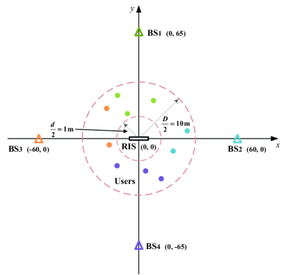
Figure 2: An illustration of the position of BSs, RIS, and users.

In addition, the path loss is modeled as $L(d)=C_{0}(\frac{d}{D_{0}})^{-\alpha}$, where $d$ is the distance, $C_{0}$ and $D_{0}$ are set as $-30\text{ dB}$ and $1\text{ m}$, respectively [12]. The path loss exponents are set as 3.5, 2.5 and 2.8 for the BS-user, BS-RIS, and RIS-user channels, respectively. Moreover, the Rician channel model is considered in the simulation studies. The BS-user channels are assumed as Non-Line-of-Sight (NLoS) channels because of the complex wireless propagation environment between BSs and users. Since RIS is usually deployed at high buildings, there exist strong Line-of-Sight (LoS) channels between BSs and RIS. Furthermore, the RIS-user channels consist both LoS links and NLoS links since the RIS is set nearby the users. Thus, we set the Rician factors as 0, $\infty$, and 1 for the BS-user, BS-RIS, and RIS-user channels, respectively.

We first present the convergence performance of the proposed FP-MM-ADMM based joint association and beamforming design algorithm by plotting the objective value of (30a) and sum-rate versus the number of iterations in Fig. 3, respectively. To be specific, Fig. 3(a) verifies the convergence of the first loop of Algorithm 1 and Fig. 3(b) demonstrates the convergence of Algorithm 2. It can be seen that the convergence can be achieved within a limited number of iterations under different settings.

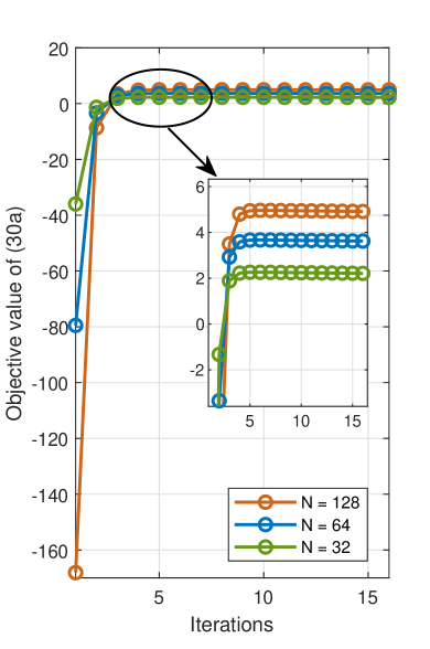
(a) First inner loop.

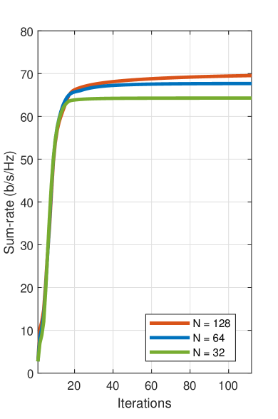
(b) Outer loop.

Figure 3: Convergence of proposed algorithm.

Then, the association results of our proposed algorithm is shown in Fig. 4, in which different colors represent different BSs as well as their associated RIS and users. We can observe that the RIS is associated to BS2, i.e., the blue BS, which can significantly enlarge the coverage area of this cell. Thus, more users are associated to BS2 to achieve better sum-rate performance. Moreover, it is obvious that BS1, i.e., the green BS, is associated with less users due to the worst channel gain.

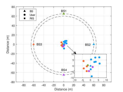
Figure 4: Association results ($P_{\text{max}}=20\text{dBm}$, $M=32$, $N=64$, $K=15$).

Fig. 5 evaluates the proposed algorithm by showing the sum-rate versus the maximum transmit power $P_{\text{max}}$. For comparison purpose, we also include the traditional direct channel gain based user association scheme, which determines the BS-user association only based on the channel gain of the direct BS-user channels [50], [51] and optimizes the BS-RIS association by the proposed ADMM based passive beamforming design algorithm. Since the gain-based algorithm only considers the direct BS-user channels, the resulting BS-user association will not be affected by the deployment of RIS. To better demonstrate the advantages of the proposed joint BS-RIS-user association and beamforming design, these two schemes are compared under three scenarios. i) With RIS (w/ RIS): A RIS is deployed in the network, the BS-RIS association and its passive beamforming are optimized; ii) Random RIS (r/ RIS): A RIS is deployed in the network, but the BS-RIS association and its passive beamforming are randomly generated; iii) Without RIS (w/o RIS): The case without deploying RIS. It can be observed from Fig. 5 that the “w/ RIS” and “r/ RIS” schemes outperform the “w/o RIS” scheme, which demonstrates the advantage of deploying RIS in the multi-cell wireless communication network. Moreover, the proposed algorithm can achieve better performance compared with the gain-based association algorithm for all power ranges. This is because the gain-based association algorithm only considers the BS-user channel gain and ignores the impact of the BS-RIS-user cascaded channel in the process of BS-user association, which causes significant performance loss. Furthermore, Fig. 5 shows that the performance gap between “w/ RIS” and “w/o RIS” schemes for the proposed algorithm is larger than that for the gain-based algorithm, which further verifies the importance of the joint design of BS-RIS-user association and beamforming.

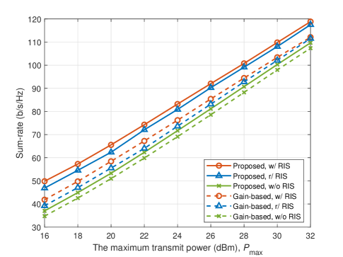
Figure 5: Sum-rate versus the maximum transmit power, $P_{\text{max}}$ ($M=32$, $N=64$, $K=15$).

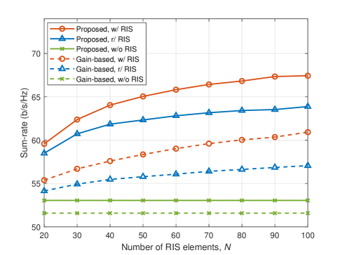
Figure 6: Sum-rate versus the number of RIS reflecting elements, $N$ ($P_{\text{max}}=20\text{dBm}$, $M=32$, $K=15$).

Then, the sum-rate versus the number of RIS reflecting elements $N$ is plotted in Fig. 6. Similar conclusions can be drawn that the deployment of RIS will promote the system performance and the proposed algorithm can achieve better performance than its competitors. Moreover, benefiting from larger gain of passive beamforming provided by more reflecting elements, the sum-rate of all schemes increases with the increasing of $N$.

Fig. 7 describes the sum-rate as a function of the number of users $K$. We observe that the sum-rate of all schemes increases with increasing $K$, since larger multi-user diversity is brought by more users. In addition, it is obvious that the performance improvement of sum-rate becomes saturated when users are very dense due to limited network resources to allocate to each user and larger multi-user interference. Moreover, our proposed algorithm remains better performance compared with the gain-based algorithm for different numbers of users. Since the gain-based user association algorithm only determines the BS-user association based on the direct channel gain, more users will be associated with the closer BSs, i.e., BS2 and BS3. Thus, less power will be allocated to each user associated with these two BSs when more users are distributed in the network, which significantly degrades the sum-rate performance.

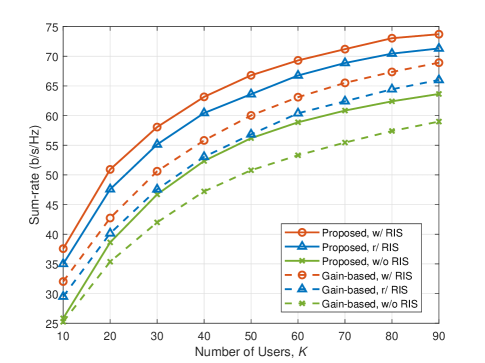
Figure 7: Sum-rate versus the number of users, $K$ ($P_{\text{max}}=15\text{dBm}$, $M=32$, $N=64$).

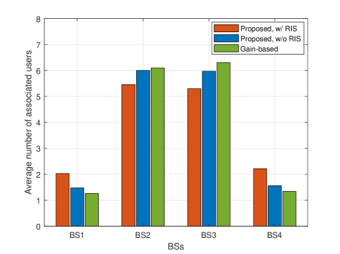
Figure 8: Average number of users served by each BS ($P_{\text{max}}=20\text{dBm}$, $M=32$, $N=64$, $K=15$).

Thus, in Fig. 8, we present the average number of users served by each BS of different algorithms under different scenarios, in which BS1 and BS4 are at relatively farther distances away from users. We only plot the “gain-based” result in this figure since the resulting BS-user association of gain-based algorithm will not be affected by the deployment of RIS, as we analysed before. It can be easily observed that with the deployment of RIS, the BSs far away from users, i.e., BS1 and BS4, can serve more users than the system without RIS by comparing the “proposed, w/ RIS” and “proposed, w/o RIS” schemes. This phenomenon verifies that the deployment of RIS can expand cell coverage in cellular networks. Moreover, it is obvious that more users will be associated with farther BSs by utilizing the proposed algorithm compared with gain-based algorithm. These facts demonstrate that the deployment of RIS and the proposed joint BS-RIS-user association design can facilitate the load balancing between BSs, which is beneficial to the utilization of resources.

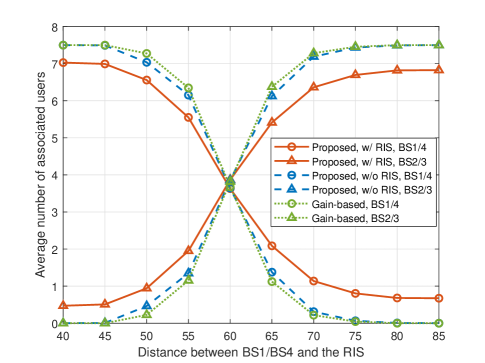
Figure 9: Average number of associated users versus the distance between BS1/BS4 and the RIS ($P_{\text{max}}=20\text{dBm}$, $M=32$, $N=64$, $K=15$).

To further demonstrate the advantages of our proposed algorithm for load balancing, the average number of associated users versus the distance between BS1/BS4 and RIS is plotted in Fig. 9. According to the geometry positions presented in Fig. 2, BS1 and BS4 will achieve the same performance under the same settings, and so will BS2 and BS3. Thus, we only plot two curves under each scheme in Fig. 9. To be specific, the curve “BS1/4” is the average number of users associated with BS1 and BS4, while the curve “BS2/3” is the average number of users associated with BS2 and BS3. We can observe that the proposed algorithm will associate more users to farther BSs and less users to closer BSs compared with gain-based algorithm in all distance ranges. Moreover, the average number of associated users with different BSs gets closer when the distance from the BSs to the RIS tends to be equal to $60$m. These facts further verify the load balancing ability of the proposed algorithm and the cell edge expansion by deploying RIS in cellular networks.

V Conclusion

In this paper, we considered a practical RIS-assisted multi-cell wireless network and investigated to maximize the sum-rate by jointly optimizing the BS-RIS-user association, the active beamforming at BSs, as well as the passive beamforming of RIS. An efficient joint association and beamforming optimization algorithm exploiting FP, MM and ADMM methods was developed to solve this complicated non-convex problem. Simulation results demonstrated the effectiveness and the performance improvement of our proposed algorithm. To be specific, the deployment of RIS with the proposed joint association and beamforming design algorithm can expand the cell coverage, facilitate the load balancing between BSs, and consequently promotes the performance of cellular network. For the future studies, it would be significative to extend the proposed joint BS-RIS-user association and beamforming design architecture to multi-RIS assisted multi-cell multi-user systems. Moreover, the fairness among users is also a worth studying issue as the extended research directions.

Appendix A Proof of Proposition 1

$$-\mathcal{H}_{\mathbf{w}_{j,k},\mathbf{w}_{j,k}^{*}}g_{\delta}\left(\mathbf{w}_{j,k},\mathbf{w}_{j,k}^{*}\right) =\exp\Big{(}-\frac{\|\mathbf{w}_{j,k}\|_{2}^{2}}{\delta}\Big{)}\Big{(}\frac{1}{\delta^{2}}\mathbf{w}_{j,k}\mathbf{w}_{j,k}^{H}-\frac{1}{\delta}\mathbf{I}_{M}\Big{)},$$ (54a)

$$-\mathcal{H}_{\mathbf{w}_{j,k}^{*},\mathbf{w}_{j,k}^{*}}g_{\delta}\left(\mathbf{w}_{j,k},\mathbf{w}_{j,k}^{*}\right) =\exp\Big{(}-\frac{\|\mathbf{w}_{j,k}\|_{2}^{2}}{\delta}\Big{)}\Big{(}\frac{1}{\delta^{2}}\mathbf{w}_{j,k}\mathbf{w}_{j,k}^{T}\Big{)},$$ (54b)

$$-\mathcal{H}_{\mathbf{w}_{j,k},\mathbf{w}_{j,k}}g_{\delta}\left(\mathbf{w}_{j,k},\mathbf{w}_{j,k}^{*}\right) =\exp\Big{(}-\frac{\|\mathbf{w}_{j,k}\|_{2}^{2}}{\delta}\Big{)}\Big{(}\frac{1}{\delta^{2}}\mathbf{w}_{j,k}^{*}\mathbf{w}_{j,k}^{H}\Big{)},$$ (54c)

$$-\mathcal{H}_{\mathbf{w}_{j,k}^{*},\mathbf{w}_{j,k}}g_{\delta}\left(\mathbf{w}_{j,k},\mathbf{w}_{j,k}^{*}\right) =\exp\Big{(}-\frac{\|\mathbf{w}_{j,k}\|_{2}^{2}}{\delta}\Big{)}\Big{(}\frac{1}{\delta^{2}}\mathbf{w}_{j,k}^{*}\mathbf{w}_{j,k}^{T}-\frac{1}{\delta}\mathbf{I}_{M}\Big{)}.$$ (54d)

$$-\mathcal{H}_{\boldsymbol{\varphi}_{j},\boldsymbol{\varphi}_{j}^{*}}g_{\delta}(\boldsymbol{\varphi}_{j},\boldsymbol{\varphi}_{j}^{*})= \varepsilon_{j}\Big{(}\frac{1}{\delta^{2}}\left((\ln(\boldsymbol{\varphi}_{j}))\oslash\boldsymbol{\varphi}_{j}^{*}\right)\left((\ln(\boldsymbol{\varphi}_{j}))^{H}\oslash\boldsymbol{\varphi}_{j}^{T}\right)-\frac{1}{\delta}\operatorname{diag}\{\mathbf{1}_{N}\oslash\boldsymbol{\varphi}_{j}\oslash\boldsymbol{\varphi}_{j}^{*}\}\Big{)},$$ (62a)

$$-\mathcal{H}_{\boldsymbol{\varphi}_{j}^{*},\boldsymbol{\varphi}_{j}^{*}}g_{\delta}(\boldsymbol{\varphi}_{j},\boldsymbol{\varphi}_{j}^{*})= \varepsilon_{j}\Big{(}\frac{1}{\delta^{2}}\left((\ln(\boldsymbol{\varphi}_{j}))\oslash\boldsymbol{\varphi}_{j}^{*}\right)\left((\ln(\boldsymbol{\varphi}_{j}))^{T}\oslash\boldsymbol{\varphi}_{j}^{H}\right)-\frac{1}{\delta}\operatorname{diag}\{\ln(\boldsymbol{\varphi}_{j})\oslash\boldsymbol{\varphi}_{j}^{*}\oslash\boldsymbol{\varphi}_{j}^{*}\}\Big{)},$$ (62b)

$$-\mathcal{H}_{\boldsymbol{\varphi}_{j},\boldsymbol{\varphi}_{j}}g_{\delta}(\boldsymbol{\varphi}_{j},\boldsymbol{\varphi}_{j}^{*})= \varepsilon_{j}\Big{(}\frac{1}{\delta^{2}}\left((\ln(\boldsymbol{\varphi}_{j}^{*}))\oslash\boldsymbol{\varphi}_{j}\right)\left((\ln(\boldsymbol{\varphi}_{j}))^{H}\oslash\boldsymbol{\varphi}_{j}^{T}\right)-\frac{1}{\delta}\operatorname{diag}\{\ln(\boldsymbol{\varphi}_{j}^{*})\oslash\boldsymbol{\varphi}_{j}\oslash\boldsymbol{\varphi}_{j}\}\Big{)},$$ (62c)

$$-\mathcal{H}_{\boldsymbol{\varphi}_{j}^{*},\boldsymbol{\varphi}_{j}}g_{\delta}(\boldsymbol{\varphi}_{j},\boldsymbol{\varphi}_{j}^{*})= \varepsilon_{j}\Big{(}\frac{1}{\delta^{2}}\left((\ln(\boldsymbol{\varphi}_{j}^{*}))\oslash\boldsymbol{\varphi}_{j}\right)\left((\ln(\boldsymbol{\varphi}_{j}))^{T}\oslash\boldsymbol{\varphi}_{j}^{H}\right)-\frac{1}{\delta}\operatorname{diag}\{\mathbf{1}_{N}\oslash\boldsymbol{\varphi}_{j}^{*}\oslash\boldsymbol{\varphi}_{j}\}\Big{)}.$$ (62d)

Since $-g_{\delta}(\|\mathbf{w}_{j,k}\|_{2}^{2})$ is twice differentiable, inspired by [47], the second-order Taylor expansion is utilized to construct its upper-bound $\widetilde{g}_{\delta}(\mathbf{w}_{j,k}|\mathbf{w}_{j,k}^{(t-1)})$. As introduced in [52], the second-order Taylor series of function $-g_{\delta}\left(\|\mathbf{w}_{j,k}\|_{2}^{2}\right)$ at point $\mathbf{w}_{j,k}$ can be written as

$$H_{1}\left(\mathbf{w}_{j,k}\right)= -g_{\delta}(\|\mathbf{w}_{j,k}^{(t-1)}\|_{2}^{2})-\left(\mathcal{D}_{\mathbf{w}_{j,k}}g_{\delta}(\mathbf{w}_{j,k},\mathbf{w}_{j,k}^{*})\right)d\mathbf{w}_{j,k}$$ (50)

$$-\left(\mathcal{D}_{\mathbf{w}_{j,k}^{*}}g_{\delta}(\mathbf{w}_{j,k},\mathbf{w}_{j,k}^{*})\right)d\mathbf{w}_{j,k}^{*}$$

$$+\frac{1}{2}\left[d\mathbf{w}_{j,k}^{H}~{}~{}d\mathbf{w}_{j,k}^{T}\right]\mathcal{H}_{j,k}\left[\begin{array}[]{c}d\mathbf{w}_{j,k}\\ d\mathbf{w}_{j,k}^{*}\end{array}\right],$$

in which $\mathcal{D}_{\mathbf{w}_{j,k}}g_{\delta}(\mathbf{w}_{j,k},\mathbf{w}_{j,k}^{*})$ and $\mathcal{D}_{\mathbf{w}_{j,k}^{*}}g_{\delta}(\mathbf{w}_{j,k},\mathbf{w}_{j,k}^{*})$ represent the complex-valued derivatives of the function $g_{\delta}(\mathbf{w}_{j,k},\mathbf{w}_{j,k}^{*})$ with respect to $\mathbf{w}_{j,k}$ and $\mathbf{w}_{j,k}^{*}$, respectively. As introduced in Lemma 5.2 [52], the complex Hessian matrix of $-g_{\delta}\left(\mathbf{w}_{j,k}\right)$ can be expressed as

$$\mathcal{H}_{j,k}=\left[\begin{array}[]{cc}-\mathcal{H}_{\mathbf{w}_{j,k},\mathbf{w}_{j,k}^{*}}g_{\delta}&-\mathcal{H}_{\mathbf{w}_{j,k}^{*},\mathbf{w}_{j,k}^{*}}g_{\delta}\\ -\mathcal{H}_{\mathbf{w}_{j,k},\mathbf{w}_{j,k}}g_{\delta}&-\mathcal{H}_{\mathbf{w}_{j,k}^{*},\mathbf{w}_{j,k}}g_{\delta}\end{array}\right],$$ (51)

where $\mathcal{H}_{\mathbf{w}_{j,k},\mathbf{w}_{j,k}^{*}}g_{\delta}\triangleq\mathcal{D}_{\mathbf{w}_{j,k}}(\mathcal{D}_{\mathbf{w}_{j,k}^{*}}g_{\delta}(\mathbf{w}_{j,k},\mathbf{w}_{j,k}^{*}))^{T}$ represents the complex Hessian matrix for function $g_{\delta}(\mathbf{w}_{j,k},\mathbf{w}_{j,k}^{*})$ with respect to $(\mathbf{w}_{j,k},\mathbf{w}_{j,k}^{*})$, and similar definitions for the other matrices in $\mathcal{H}_{j,k}$. Based on the definition

$$-g_{\delta}\left(\|\mathbf{w}_{j,k}\|_{2}^{2}\right)=\exp\big{(}-\frac{\left\|\mathbf{w}_{j,k}\right\|_{2}^{2}}{\delta}\big{)}-1,$$ (52)

we can obtain the derivatives

$$-\mathcal{D}_{\mathbf{w}_{j,k}}g_{\delta}\left(\mathbf{w}_{j,k},\mathbf{w}_{j,k}^{*}\right)= -\frac{1}{\delta}\exp\Big{(}-\frac{\left\|\mathbf{w}_{j,k}\right\|_{2}^{2}}{\delta}\Big{)}\mathbf{w}_{j,k}^{H},$$ (53a)

$$-\mathcal{D}_{\mathbf{w}_{j,k}^{*}}g_{\delta}\left(\mathbf{w}_{j,k},\mathbf{w}_{j,k}^{*}\right)= -\frac{1}{\delta}\exp\Big{(}-\frac{\left\|\mathbf{w}_{j,k}\right\|_{2}^{2}}{\delta}\Big{)}\mathbf{w}_{j,k}^{T},$$ (53b)

and Hessian matrices (54) as shown on the top of next page.

Then, to construct an upper-bound of $H_{1}\left(\mathbf{w}_{j,k}\right)$ at point $\mathbf{w}_{j,k}$, a matrix $\widetilde{\mathbf{M}}_{j,k}$, which satisfies $\widetilde{\mathbf{M}}_{j,k}\succeq\mathcal{H}_{j,k}$, needs to be adopted. Thus, we set

$$\widetilde{\mathbf{M}}_{j,k}=\left[\begin{array}[]{cc}\mathbf{M}_{j,k}&\mathbf{0}_{M\times M}\\ \mathbf{0}_{M\times M}&\mathbf{M}_{j,k}^{T}\end{array}\right]=\max{\{0,\lambda_{j,k}\}}\cdot\mathbf{I}_{2M},$$ (55)

where $\lambda_{j,k}$ is the maximum eigenvalue of the matrix $\mathcal{H}_{j,k}$. Moreover, $d\mathbf{w}_{j,k}$ equals to $\mathbf{w}_{j,k}-\mathbf{w}_{j,k}^{(t-1)}$. Finally, a convex upper-bound $\widetilde{g}_{\delta}(\mathbf{w}_{j,k}|\mathbf{w}_{j,k}^{(t-1)})$ can be written as

$$\widetilde{g}_{\delta}(\mathbf{w}_{j,k}|\mathbf{w}_{j,k}^{(t-1)})= \mathfrak{Re}\{\mathbf{w}_{j,k}^{H}\mathbf{M}_{j,k}\mathbf{w}_{j,k}\}+\mathfrak{Re}\{\boldsymbol{\iota}_{j,k}^{H}\mathbf{w}_{j,k}\}$$ (56)

$$+\varpi_{j,k},~{}\forall j,~{}\forall k,$$

in which

$$\mathbf{M}_{j,k}\triangleq \max{\{0,\lambda_{j,k}\}}\cdot\mathbf{I}_{M},~{}\forall j,\forall k,$$ (57a)

$$\beta_{j,k}^{(t-1)}\triangleq \frac{1}{\delta}\exp\Big{(}-\frac{\big{\|}\mathbf{w}_{j,k}^{(t-1)}\big{\|}_{2}^{2}}{\delta}\Big{)},~{}\forall j,\forall k,$$ (57b)

$$\boldsymbol{\iota}_{j,k}^{H}\triangleq -2(\mathbf{w}_{j,k}^{(t-1)})^{H}\mathbf{M}_{j,k}-2\beta_{j,k}^{(t-1)}(\mathbf{w}_{j,k}^{(t-1)})^{H},~{}\forall j,\forall k,$$ (57c)

$$\varpi_{j,k}\triangleq -h_{\delta}(\|\mathbf{w}_{j,k}^{(t-1)}\|_{2}^{2})+\mathfrak{Re}\{(\mathbf{w}_{j,k}^{(t-1)})^{H}\mathbf{M}_{j,k}\mathbf{w}_{j,k}^{(t-1)}\}$$ (57d)

$$+2\mathfrak{Re}\{\beta_{j,k}^{(t-1)}(\mathbf{w}_{j,k}^{(t-1)})^{H}\mathbf{w}_{j,k}^{(t-1)}\},\forall j,\forall k.$$

Hence, Proposition 1 is proved. $\blacksquare$

Appendix B Proof of Proposition 2

Since $-g_{\delta}\left(\|\ln(\boldsymbol{\varphi}_{j})\|_{2}^{2}\right)$ is twice differentiable, the second-order Taylor expansion of $-g_{\delta}\left(\|\ln(\boldsymbol{\varphi}_{j})\|_{2}^{2}\right)$ at point $\boldsymbol{\varphi}_{j}$ can be adopted as

$$H_{2}(\boldsymbol{\varphi}_{j})= -g_{\delta}\left(\|\ln(\boldsymbol{\varphi}_{j})^{(t-1)}\|_{2}^{2}\right)-(\mathcal{D}_{\boldsymbol{\varphi}_{j}}g_{\delta}(\boldsymbol{\varphi}_{j},\boldsymbol{\varphi}_{j}^{*}))d\boldsymbol{\varphi}_{j}$$ (58)

$$-(\mathcal{D}_{\boldsymbol{\varphi}_{j}^{*}}g_{\delta}(\boldsymbol{\varphi}_{j},\boldsymbol{\varphi}_{j}^{*}))d\boldsymbol{\varphi}_{j}^{*}$$

$$+\frac{1}{2}\left[d\boldsymbol{\varphi}_{j}^{H}~{}~{}d\boldsymbol{\varphi}_{j}^{T}\right]\mathcal{H}_{j}\left[\begin{array}[]{c}d\boldsymbol{\varphi}_{j}\\ d\boldsymbol{\varphi}_{j}^{*}\end{array}\right],$$

in which similar definitions for the derivatives and Hessian matrices as that in (50) are used, and

$$\mathcal{H}_{j}=\left[\begin{array}[]{cc}-\mathcal{H}_{\boldsymbol{\varphi}_{j},\boldsymbol{\varphi}_{j}^{*}}g_{\delta}&-\mathcal{H}_{\boldsymbol{\varphi}_{j}^{*},\boldsymbol{\varphi}_{j}^{*}}g_{\delta}\\ -\mathcal{H}_{\boldsymbol{\varphi}_{j},\boldsymbol{\varphi}_{j}}g_{\delta}&-\mathcal{H}_{\boldsymbol{\varphi}_{j}^{*},\boldsymbol{\varphi}_{j}}g_{\delta}\end{array}\right],$$ (59)

is the complex Hessian matrix of $-g_{\delta}(\|\ln(\boldsymbol{\varphi}_{j})\|_{2}^{2})$. Then, based on the defination

$$-g_{\delta}(\|\ln(\boldsymbol{\varphi}_{j})\|_{2}^{2})=\exp\Big{(}-\frac{\|\ln(\boldsymbol{\varphi}_{j})\|_{2}^{2}}{\delta}\Big{)}-1,$$ (60)

we can obtain

$$-\mathcal{D}_{\boldsymbol{\varphi}_{j}}g_{\delta}(\boldsymbol{\varphi}_{j},\boldsymbol{\varphi}_{j}^{*})= -\frac{1}{\delta}\exp(-\frac{\|\ln(\boldsymbol{\varphi}_{j})\|_{2}^{2}}{\delta})((\ln(\boldsymbol{\varphi}_{j}))^{H}\oslash\boldsymbol{\varphi}_{j}^{T}),$$ (61a)

$$-\mathcal{D}_{\boldsymbol{\varphi}_{j}^{*}}g_{\delta}(\boldsymbol{\varphi}_{j},\boldsymbol{\varphi}_{j}^{*})= -\frac{1}{\delta}\exp(-\frac{\|\ln(\boldsymbol{\varphi}_{j})\|_{2}^{2}}{\delta})((\ln(\boldsymbol{\varphi}_{j}))^{T}\oslash\boldsymbol{\varphi}_{j}^{H}),$$ (61b)

and (62) as shown on the top of this page, in which $\oslash$ presents the element-wise division and for brevity we define

$$\varepsilon_{j}\triangleq\frac{1}{\delta}\exp\Big{(}-\frac{\big{\|}\ln(\boldsymbol{\varphi}_{j})\big{\|}_{2}^{2}}{\delta}\Big{)}.$$ (63)

To construct the upper-bound $\overline{g}_{\delta}(\boldsymbol{\varphi}_{j}|\boldsymbol{\varphi}_{j}^{(t-1)})$, the matrix

$$\widetilde{\boldsymbol{\Xi}}_{j}=\left[\begin{array}[]{cc}\boldsymbol{\Xi}_{j}&\mathbf{0}_{N\times N}\\ \mathbf{0}_{N\times N}&\boldsymbol{\Xi}_{j}^{T}\end{array}\right]=\max{\{0,\lambda_{j}\}}\cdot\mathbf{I}_{2N},$$ (64)

is utilized as the upper-bound of the Hessian matrix $\mathcal{H}_{j}$ in (58), which satisfies the constraint $\widetilde{\boldsymbol{\Xi}}_{j}\succeq\mathcal{H}_{j}$. Here, $\lambda_{j}$ is the maximum eigenvalue of the matrix $\mathcal{H}_{j}$. Finally, by substituting (61), (62), and $d\boldsymbol{\varphi}_{j}=\boldsymbol{\varphi}_{j}-\boldsymbol{\varphi}_{j}^{(t-1)}$ into (58), the upper-bound $\overline{g}_{\delta}(\boldsymbol{\varphi}_{j}|\boldsymbol{\varphi}_{j}^{(t-1)})$ can be given by

$$\overline{g}_{\delta}(\boldsymbol{\varphi}_{j}|\boldsymbol{\varphi}_{j}^{(t-1)})=\mathfrak{Re}\{\boldsymbol{\varphi}_{j}^{H}\boldsymbol{\Xi}_{j}\boldsymbol{\varphi}_{j}\}+\mathfrak{Re}\{\boldsymbol{\kappa}_{j}^{H}\boldsymbol{\varphi}_{j}\}+\mu_{j},\forall j,$$ (65)

in which

$$\mathbf{\Xi}_{j}\triangleq \max{\{0,\lambda_{j}\}}\cdot\mathbf{I}_{N},~{}\forall j,$$ (66a)

$$\boldsymbol{\kappa}_{j}\triangleq -2(\boldsymbol{\varphi}_{j}^{(t-1)})^{H}\boldsymbol{\Xi}_{j}-2\varepsilon_{j}^{(t-1)}(\boldsymbol{\phi}_{j}^{(t-1)})^{H},~{}\forall j,$$ (66b)

$$\mu_{j}\triangleq -g_{\delta}(\|\ln(\boldsymbol{\varphi}_{j}^{(t-1)})\|_{2}^{2})+\mathfrak{Re}\{(\boldsymbol{\varphi}_{j}^{(t-1)})^{H}\boldsymbol{\Xi}_{j}\boldsymbol{\varphi}_{j}^{(t-1)}\}$$ (66c)

$$+2\mathfrak{Re}\{\varepsilon_{j}^{(t-1)}(\boldsymbol{\phi}_{j}^{(t-1)})^{H}\boldsymbol{\varphi}_{j}^{(t-1)}\},~{}\forall j.$$

Here, for brevity we define

$$\varepsilon_{j}^{(t-1)}\triangleq \frac{1}{\delta}\exp\Big{(}-\frac{\big{\|}\ln(\boldsymbol{\varphi}_{j}^{(t-1)})\big{\|}_{2}^{2}}{\delta}\Big{)},~{}\forall j,$$ (67a)

$$(\boldsymbol{\phi}_{j}^{(t-1)})^{H}\triangleq \ln({\boldsymbol{\varphi}_{j}^{(t-1)})}^{H}\oslash{(\boldsymbol{\varphi}_{j}^{(t-1)})}^{T},~{}\forall j.$$ (67b)

Now, the proof of Proposition 2 is complete. $\blacksquare$

Appendix C Proof of Proposition 3

$$\mathcal{H}_{\boldsymbol{\varphi}_{j},\boldsymbol{\varphi}_{j}^{*}}g_{\delta}(\boldsymbol{\varphi}_{j},\boldsymbol{\varphi}_{j}^{*})= \varepsilon_{j}\Big{(}\frac{1}{\delta}\operatorname{diag}\{\mathbf{1}_{N}\oslash\boldsymbol{\varphi}_{j}\oslash\boldsymbol{\varphi}_{j}^{*}\}-\frac{1}{\delta^{2}}\left((\ln(\boldsymbol{\varphi}_{j}))\oslash\boldsymbol{\varphi}_{j}^{*}\right)\left((\ln(\boldsymbol{\varphi}_{j}))^{H}\oslash\boldsymbol{\varphi}_{j}^{T}\right)\Big{)},$$ (71a)

$$\mathcal{H}_{\boldsymbol{\varphi}_{j}^{*},\boldsymbol{\varphi}_{j}^{*}}g_{\delta}(\boldsymbol{\varphi}_{j},\boldsymbol{\varphi}_{j}^{*})= \varepsilon_{j}\Big{(}\frac{1}{\delta}\operatorname{diag}\{\ln(\boldsymbol{\varphi}_{j})\oslash\boldsymbol{\varphi}_{j}^{*}\oslash\boldsymbol{\varphi}_{j}^{*}\}-\frac{1}{\delta^{2}}\left((\ln(\boldsymbol{\varphi}_{j}))\oslash\boldsymbol{\varphi}_{j}^{*}\right)\left((\ln(\boldsymbol{\varphi}_{j}))^{T}\oslash\boldsymbol{\varphi}_{j}^{H}\right)\Big{)},$$ (71b)

$$\mathcal{H}_{\boldsymbol{\varphi}_{j},\boldsymbol{\varphi}_{j}}g_{\delta}(\boldsymbol{\varphi}_{j},\boldsymbol{\varphi}_{j}^{*})= \varepsilon_{j}\Big{(}\frac{1}{\delta}\operatorname{diag}\{\ln(\boldsymbol{\varphi}_{j}^{*})\oslash\boldsymbol{\varphi}_{j}\oslash\boldsymbol{\varphi}_{j}\}-\frac{1}{\delta^{2}}\left((\ln(\boldsymbol{\varphi}_{j}^{*}))\oslash\boldsymbol{\varphi}_{j}\right)\left((\ln(\boldsymbol{\varphi}_{j}))^{H}\oslash\boldsymbol{\varphi}_{j}^{T}\right)\Big{)},$$ (71c)

$$\mathcal{H}_{\boldsymbol{\varphi}_{j}^{*},\boldsymbol{\varphi}_{j}}g_{\delta}(\boldsymbol{\varphi}_{j},\boldsymbol{\varphi}_{j}^{*})= \varepsilon_{j}\Big{(}\frac{1}{\delta}\operatorname{diag}\{\mathbf{1}_{N}\oslash\boldsymbol{\varphi}_{j}^{*}\oslash\boldsymbol{\varphi}_{j}\}-\frac{1}{\delta^{2}}\left((\ln(\boldsymbol{\varphi}_{j}^{*}))\oslash\boldsymbol{\varphi}_{j}\right)\left((\ln(\boldsymbol{\varphi}_{j}))^{T}\oslash\boldsymbol{\varphi}_{j}^{H}\right)\Big{)}.$$ (71d)

Similar to the method utilized to construct $\overline{g}_{\delta}(\boldsymbol{\varphi}_{j}|\boldsymbol{\varphi}_{j}^{(t-1)})$, we can construct a convex function $\breve{g}_{\delta}(\boldsymbol{\varphi}_{j}|\boldsymbol{\varphi}_{j}^{(t-1)})$ as the upper-bound of $g_{\delta}\left(\|\ln(\boldsymbol{\varphi}_{j})\|_{2}^{2}\right)$ at point $\boldsymbol{\varphi}_{j}$ based on the second-order Taylor expansion, which is written as

$$H_{3}(\boldsymbol{\varphi}_{j})= g_{\delta}(\|\ln(\boldsymbol{\varphi}_{j}^{(t-1)})\|_{2}^{2})+\mathcal{D}_{\boldsymbol{\varphi}_{j}}g_{\delta}(\boldsymbol{\varphi}_{j},\boldsymbol{\varphi}_{j}^{*})d\boldsymbol{\varphi}_{j}$$ (68)

$$+\mathcal{D}_{\boldsymbol{\varphi}_{j}^{*}}g_{\delta}(\boldsymbol{\varphi}_{j},\boldsymbol{\varphi}_{j}^{*})d\boldsymbol{\varphi}_{j}^{*}$$

$$+\frac{1}{2}\left[d\boldsymbol{\varphi}_{j}^{H}~{}~{}d\boldsymbol{\varphi}_{j}^{T}\right]\mathcal{H}_{j}\left[\begin{array}[]{c}d\boldsymbol{\varphi}_{j}\\ d\boldsymbol{\varphi}_{j}^{*}\end{array}\right],$$

in which

$$\mathcal{H}_{j}=\left[\begin{array}[]{cc}\mathcal{H}_{\boldsymbol{\varphi}_{j},\boldsymbol{\varphi}_{j}^{*}}g_{\delta}&\mathcal{H}_{\boldsymbol{\varphi}_{j}^{*},\boldsymbol{\varphi}_{j}^{*}}g_{\delta}\\ \mathcal{H}_{\boldsymbol{\varphi}_{j},\boldsymbol{\varphi}_{j}}g_{\delta}&\mathcal{H}_{\boldsymbol{\varphi}_{j}^{*},\boldsymbol{\varphi}_{j}}g_{\delta}\end{array}\right],$$ (69)

is the complex Hessian matrix of $g_{\delta}\left(\|\ln(\boldsymbol{\varphi}_{j})\|_{2}^{2}\right)$. Then, we can obtain the complex-valued derivative and Hessian results of $g_{\delta}\left(\|\ln(\boldsymbol{\varphi}_{j})\|_{2}^{2}\right)$ by

$$\mathcal{D}_{\boldsymbol{\varphi}_{j}}g_{\delta}(\boldsymbol{\varphi}_{j},\boldsymbol{\varphi}_{j}^{*})= \frac{1}{\delta}\exp(-\frac{\|\ln(\boldsymbol{\varphi}_{j})\|_{2}^{2}}{\delta})((\ln(\boldsymbol{\varphi}_{j}))^{H}\oslash\boldsymbol{\varphi}_{j}^{T}),$$ (70a)

$$\mathcal{D}_{\boldsymbol{\varphi}_{j}^{*}}g_{\delta}(\boldsymbol{\varphi}_{j},\boldsymbol{\varphi}_{j}^{*})= \frac{1}{\delta}\exp(-\frac{\|\ln(\boldsymbol{\varphi}_{j})\|_{2}^{2}}{\delta})((\ln(\boldsymbol{\varphi}_{j}))^{T}\oslash\boldsymbol{\varphi}_{j}^{H}),$$ (70b)

and (71) as shown on the top of this page. To construct the upper-bound $\breve{g}_{\delta}(\boldsymbol{\varphi}_{j}|\boldsymbol{\varphi}_{j}^{(t-1)})$, the matrix

$$\widetilde{\boldsymbol{\Gamma}}_{j}=\left[\begin{array}[]{cc}\boldsymbol{\Gamma}_{j}&\mathbf{0}_{N\times N}\\ \mathbf{0}_{N\times N}&\boldsymbol{\Gamma}_{j}^{T}\end{array}\right]=\max{\{0,\lambda_{j}\}}\cdot\mathbf{I}_{2N},$$ (72)

is utilized as the upper-bound of Hessian matrix $\mathcal{H}_{j}$ in (68), which satisfies the constraint $\widetilde{\boldsymbol{\Gamma}}_{j}\succeq\mathcal{H}_{j}$. Here, $\lambda_{j}$ is the maximum eigenvalue of matrix $\mathcal{H}_{j}$. Finally, by substituting (70), (71), and $d\boldsymbol{\varphi}_{j}=\boldsymbol{\varphi}_{j}-\boldsymbol{\varphi}_{j}^{(t-1)}$ into (68), the upper-bound $\breve{g}_{\delta}(\boldsymbol{\varphi}_{j}|\boldsymbol{\varphi}_{j}^{(t-1)})$ can be given by

$$\breve{g}_{\delta}(\boldsymbol{\varphi}_{j}|\boldsymbol{\varphi}_{j}^{(t-1)})=\mathfrak{Re}\{\boldsymbol{\varphi}_{j}^{H}\boldsymbol{\Gamma}_{j}\boldsymbol{\varphi}_{j}\}+\mathfrak{Re}\{\boldsymbol{\zeta}_{j}^{H}\boldsymbol{\varphi}_{j}\}+\eta_{j},\forall j,$$ (73)

where

$$\mathbf{\Gamma}_{j}\triangleq \max{\{0,\lambda_{j}\}}\cdot\mathbf{I}_{N},~{}\forall j,$$ (74a)

$$\boldsymbol{\zeta}_{j}^{H}\triangleq -2(\boldsymbol{\varphi}_{j}^{(t-1)})^{H}\boldsymbol{\Gamma}_{j}+2\varepsilon_{j}^{(t-1)}(\boldsymbol{\phi}_{j}^{(t-1)})^{H},~{}\forall j,$$ (74b)

$$\eta_{j}\triangleq g_{\delta}(\|\ln(\boldsymbol{\varphi}_{j}^{(t-1)})\|_{2}^{2})+\mathfrak{Re}\{(\boldsymbol{\varphi}_{j}^{(t-1)})^{H}\boldsymbol{\Gamma}_{j}\boldsymbol{\varphi}_{j}^{(t-1)}\}$$ (74c)

$$-2\mathfrak{Re}\{\varepsilon_{j}^{(t-1)}(\boldsymbol{\phi}_{j}^{(t-1)})^{H}\boldsymbol{\varphi}_{j}^{(t-1)}\},~{}\forall j.$$

The proof of Proposition 3 is complete. $\blacksquare$

References

• [1] C. Pan et al., โ€œAn overview of signal processing techniques for RIS/IRS-aided wireless systems,โ€ IEEE J. Sel. Topics Signal Process., vol. 16, no. 5, pp. 883-917, Aug. 2022.
• [2] Q. Wu and R. Zhang, โ€œTowards smart and reconfigurable environment: Intelligent reflecting surface aided wireless network,โ€ IEEE Commun. Mag., vol. 58, no. 1, pp. 106-112, Jan. 2020.
• [3] Q. Wu, S. Zhang, B. Xiong, C. You, and R. Zhang, โ€œIntelligent reflecting surface aided wireless communications: A tutorial,โ€ IEEE Trans. Commun., vol. 69, no. 5, pp. 3313-3351, May 2021.
• [4] E. Basar, M. Di Renzo, J. De Rosny, M. Debbah, M.-S. Alouini, and R. Zhang, โ€œWireless communications through reconfigurable intelligent surfaces,โ€ IEEE Access, vol. 7, pp. 116753-116773, Aug. 2019.
• [5] X. Yu, D. Xu, and R. Schober, โ€œMISO wireless communication systems via intelligent reflecting surfaces,โ€ in Proc. IEEE/CIC Int. Conf. Commun. China (ICCC), Changchun, China, Aug. 2019.
• [6] C. Huang, A. Zappone, G. C. Alexandropoulos, M. Debbah, and C. Yuen, โ€œReconfigurable intelligent surfaces for energy efficiency in wireless communication,โ€ IEEE Trans. Wireless Commun., vol. 18, no. 8, pp. 4157-4170, Aug. 2019.
• [7] G. Lee, M. Jung, A. T. Z. Kasgari, W. Saad, and M. Bennis, โ€œDeep reinforcement learning for energy-efficient networking with reconfigurable intelligent surfaces,โ€ in Proc. IEEE Int. Conf. Commun. (ICC), Dublin, Ireland, Jun. 2020.
• [8] G. Zhou, C. Pan, H. Ren, K. Wang, and A. Nallanathan, โ€œIntelligent reflecting surface aided multigroup multicast MISO communication systems,โ€ IEEE Trans. Signal Process., vol. 68, pp. 3236-3251, Apr. 2020.
• [9] S. Hu, Z. Wei, Y. Cai, D. W. K. Ng, and J. Yuan, โ€œSum-rate maximization for multiuser MISO downlink systems with self-sustainable IRS,โ€ in Proc. IEEE Global Commun. Conf. (GLOBECOM), Taipei, China, Dec. 2020.
• [10] H. Guo, Y. Liang, J. Chen, and E. G. Larsson, โ€œWeighted sum-rate maximization for reconfigurable intelligent surface aided wireless networks,โ€ IEEE Trans. Wireless Commun., vol. 19, no. 5, pp. 3064-3076, May 2020.
• [11] P. Wang, J. Fang, X. Yuan, Z. Chen, and H. Li, โ€œIntelligent reflecting surface-assisted millimeter wave communications: Joint active and passive precoding design,โ€ IEEE Trans. Veh. Technol., vol. 69, no. 12, pp. 14960-14973, Dec. 2020.
• [12] Q. Wu and R. Zhang, โ€œIntelligent reflecting surface enhanced wireless network via joint active and passive beamforming,โ€ IEEE Trans. Wireless Commun., vol. 18, no. 11, pp. 5394-5409, Nov. 2019.
• [13] Q. Wu and R. Zhang, โ€œBeamforming optimization for wireless network aided by intelligent reflecting surface with discrete phase shifts,โ€ IEEE Trans. Commun., vol. 68, no. 3, pp. 1838-1851, Mar. 2020.
• [14] M.-M. Zhao, A. Liu, Y. Wan, and R. Zhang, โ€œTwo-timescale beamforming optimization for intelligent reflecting surface aided multiuser communication with QoS constraints,โ€ IEEE Trans. Wireless Commun., vol. 20, no. 9, pp. 6179-6194, Sep. 2021.
• [15] B. Zheng, C. You, W. Mei, and R. Zhang, โ€œA survey on channel estimation and practical passive beamforming design for intelligent reflecting surface aided wireless communications,โ€ IEEE Commun. Surv. Tut., vol. 24, no. 2, pp. 1035-1071, Feb. 2022.
• [16] A. L. Swindlehurst, G. Zhou, R. Liu, C. Pan, and M. Li, โ€œChannel estimation with reconfigurable intelligent surfaces - A general framework,โ€ Proc. IEEE, vol. 110, no. 9, pp. 1312-1338, Sep. 2022.
• [17] Z. Wang, L. Liu, and S. Cui, โ€œChannel estimation for intelligent reflecting surface assisted multiuser communications: Framework, algorithms, and analysis,โ€ IEEE Trans. Wireless Commun., vol. 19, no. 10, pp. 6607-6620, Oct. 2020.
• [18] W. Yang, M. Li, and Q. Liu, โ€œA novel anchor-assisted channel estimation for RIS-aided multiuser communication systems,โ€ IEEE Commun. Lett., to appear, doi: 10.1109/LCOMM.2022.3179298.
• [19] Y. Wei, M.-M. Zhao, M.-J. Zhao, and Y. Cai, โ€œChannel estimation for IRS-aided multiuser communications with reduced error propagation,โ€ IEEE Trans. Wireless Commun., vol. 21, no. 4, pp. 2725-2741, Apr. 2022.
• [20] C. Hu, L. Dai, S. Han, and X. Wang, โ€œTwo-timescale channel estimation for reconfigurable intelligent surface aided wireless communications,โ€ IEEE Trans. Commun., vol. 69, no. 11, pp. 7736-7747, Nov. 2021.
• [21] L. Wei et al., โ€œJoint channel estimation and signal recovery for RIS-empowered multiuser communications,โ€ IEEE Trans. Commun, vol. 70, no. 7, pp. 4640-4655, Jul. 2022.
• [22] B. Zheng, Q. Wu, and R. Zhang, โ€œIntelligent reflecting surface-assisted multiple access with user pairing: NOMA or OMA?โ€ IEEE Commun. Lett., vol. 24, no. 4, pp. 753-757, Apr. 2020.
• [23] T. Hou, Y. Liu, Z. Song, X. Sun, Y. Chen, and L. Hanzo, โ€œReconfigurable intelligent surface aided NOMA networks,โ€ IEEE J. Sel. Areas Commun., vol. 38, no. 11, pp. 2575-2588, Nov. 2020.
• [24] Q. Wu and R. Zhang, โ€œWeighted sum power maximization for intelligent reflecting surface aided SWIPT,โ€ IEEE Wireless Commun. Lett., vol. 9, no. 5, pp. 586-590, May 2020.
• [25] C. Pan et al., โ€œIntelligent reflecting surface aided MIMO broadcasting for simultaneous wireless information and power transfer,โ€ IEEE J. Sel. Areas Commun., vol. 38, no. 8, pp. 1719-1734, Aug. 2020.
• [26] R. Liu, M. Li, Q. Liu, and A. L. Swindlehurst, โ€œJoint symbol-level precoding and reflecting designs for IRS-enhanced MU-MISO systems,โ€ IEEE Trans. Wireless Commun., vol. 20, no. 2, pp. 798-811, Feb. 2021.
• [27] R. Liu, M. Li, Q. Liu, and A. L. Swindlehurst, โ€œIntelligent reflecting surface based passive information transmission: A symbol-level precoding approach,โ€ IEEE Trans. Veh. Technol., vol. 70, no. 7, pp. 6735-6749, Jul. 2021.
• [28] C. Huang et al., โ€œHolographic MIMO surfaces for 6G wireless networks: Opportunities, challenges, and trends,โ€ IEEE Wireless Commun., vol. 27, no. 5, pp. 118-125, Oct. 2020.
• [29] X. Song et al., โ€œJoint transmit and reflective beamforming for IRS-assisted integrated sensing and communication,โ€ Proc. IEEE Wireless Commun. Network Conf. (WCNC), Austin, USA, Apr. 2022.
• [30] X. Wang, Z. Fei, J. Huang, and H. Yu, โ€œJoint waveform and discrete phase shift design for RIS-assisted integrated sensing and communication system under Cramรฉr-Rao bound constraint,โ€ IEEE Trans. Veh. Technol., vol. 71, no. 1, pp. 1004-1009, Jan. 2022.
• [31] Y. He, Y. Cai, H. Mao, and G. Yu, โ€œRIS-assisted communication radar coexistence: Joint beamforming design and analysis,โ€ IEEE J. Sel. Areas Commun., vol. 40, no. 7, pp. 2131-2145, Jul. 2022.
• [32] R. Liu, M. Li, Y. Liu, Q. Wu, and Q. Liu, โ€œJoint transmit waveform and passive beamforming design for RIS-aided DFRC systems,โ€ IEEE J. Sel. Topics Signal Process., vol. 16, no. 5, pp. 995-1010, Aug. 2022.
• [33] H. Li, W. Cai, Y. Liu, M. Li, Q. Liu, and Q. Wu, โ€œIntelligent reflecting surface enhanced wideband MIMO-OFDM communications: From practical model to reflection optimization,โ€ IEEE Trans. Commun., vol. 69, no. 7, pp. 4807-4820, Jul. 2021.
• [34] W. Cai, R. Liu, Y. Liu, M. Li, and Q. Liu, โ€œIntelligent reflecting surface assisted multi-cell multi-band wireless networks,โ€ in Proc. IEEE Wireless Commun. Network Conf. (WCNC), Nanjing, China, Apr. 2021.
• [35] W. Cai, H. Li, M. Li, and Q. Liu, โ€œPractical modeling and beamforming for intelligent reflecting surface aided wideband systems,โ€ IEEE Commun. Lett., vol. 24, no. 7, pp. Apr. 2020.
• [36] W. Cai, R. Liu, M. Li, Y. Liu, Q. Wu, and Q. Liu, โ€œIRS-assisted multicell multiband systems: Practical reflection model and joint beamforming design,โ€ IEEE Trans. Commun., vol. 70, no. 6, pp. 3897-3911, Jun. 2022.
• [37] E. M. Taghavi, A. Alizadeh, N. Rajatheva, M. Vu, and M. Latva-aho, โ€œUser association in millimeter wave cellular networks with intelligent reflecting surfaces,โ€ in Proc. IEEE Veh. Technol. Conf. (VTC), Helsinki, Finland, Apr. 2021.
• [38] P. Han, Z. Zhou, and Z. Wang, โ€œJoint user association and passive beamforming in heterogeneous networks with reconfigurable intelligent surfaces,โ€ IEEE Commun. Lett., vol. 25, no. 9, pp. 3041-3045, Sep. 2021.
• [39] D. Zhao, H. Lu, Y. Wang, H. Sun, and Y. Gui, โ€œJoint power allocation and user association optimization for IRS-assisted mmWave systems,โ€ IEEE Trans. Wireless Commun., vol. 21, no. 1, pp. 577-590, Jan. 2022.
• [40] D. Jin, Y. Xiao, Y. Li, G. Shi, and D. Niyato, โ€œOptimizing intelligent reflecting surface-base station association for mobile networks,โ€ in Proc IEEE Int. Conf. Commun. (ICC), Montreal, Canada, Jun. 2021.
• [41] Y. Huang, W. Mei, and R. Zhang, โ€œEmpowering base stations with co-site intelligent reflecting surfaces: User association, channel estimation and reflection optimization,โ€ IEEE Trans. Commun., to appear, doi: 10.1109/TCOMM.2022.3178762
• [42] W. Mei and R. Zhang, โ€œPerformance analysis and user association optimization for wireless network aided by multiple intelligent reflecting surfaces,โ€ IEEE Trans. Commun., vol. 69, no. 9, pp. 6296-6312, Sep. 2021.
• [43] W. Mei and R. Zhang, โ€œJoint base station-IRS-user association in multi-IRS-aided wireless network,โ€ in Proc. IEEE Global Commun. Conf. (GLOBECOM), Taipei, China, Dec. 2020.
• [44] S. Liu, P. Ni, R. Liu, Y. Liu, M. Li, and Q. Liu, โ€œBS-RIS-user association and beamforming designs for RIS-aided cellular networks,โ€ in Proc. IEEE/CIC Int. Conf. Commun. China (ICCC), Xiamen, China, Jul. 2021.
• [45] K. Shen and W. Yu, โ€œFractional programming for communication systems - Part I: Power control and beamforming,โ€ IEEE Trans. Signal Process., vol. 66, no. 10, pp. 2616-2630, May 2018.
• [46] M. Tao, E. Chen, H. Zhou, and W. Yu, โ€œContent-centric sparse multicast beamforming for cache-enabled cloud RAN,โ€ IEEE Trans. Wireless Commun., vol. 15, no. 9, pp. 6118-6131, Sep. 2016.
• [47] Y. Sun, P. Babu, and D. P. Palomar, โ€œMajorization-minimization algorithms in signal processing, communications, and machine learning,โ€ IEEE Trans. Signal Process., vol. 65, no. 3, pp. 794-816, Feb. 2017.
• [48] M. Grant and S. Boyd, โ€œCVX: MATLAB software for disciplined convex programming,โ€ 2016. [Online] Available: http://cvxr.com/cvx
• [49] S. Boyd, N. Parikh, E. Chu, B. Peleato, and J. Eckstein, โ€œDistributed optimization and statistical learning via the alternating direction method of multipliers,โ€ Found. Trends Mach. Learn., vol. 3, no. 1, pp. 1-122, Jan. 2011.
• [50] A. H. Sakr and E. Hossain, โ€œAnalysis of K-tier uplink cellular networks with ambient RF energy harvesting,โ€ IEEE J. Sel. Areas Commun., vol. 33, no. 10, pp. 2226-2238, Oct. 2015.
• [51] P. Ni, Z. Wang, H. Li, M. Li, and Q. Liu, โ€œJoint user scheduling and hybrid beamforming design for cooperative mmWave networks,โ€ in Proc. IEEE Wireless Commun. Network Conf. (WCNC), Nanjing, China, Apr. 2021.
• [52] A. Hj${\o}$rungnes, โ€œComplex-valued matrix derivatives: With applications in signal processing and communications,โ€ Cambridge, U.K.: Cambridge Univ. Press, 2011.