Distributed optimization on directed graphs based on inexact ADMM with partial participation

Abstract

We consider the problem of minimizing the sum of cost functions pertaining to agents over a network whose topology is captured by a directed graph (i.e., asymmetric communication). We cast the problem into the ADMM setting, via a consensus constraint, for which both primal subproblems are solved inexactly. In specific, the computationally demanding local minimization step is replaced by a single gradient step, while the averaging step is approximated in a distributed fashion. Furthermore, partial participation is allowed in the implementation of the algorithm. Under standard assumptions on strong convexity and Lipschitz continuous gradients, we establish linear convergence and characterize the rate in terms of the connectivity of the graph and the conditioning of the problem. Our line of analysis provides a sharper convergence rate compared to Push-DIGing. Numerical experiments corroborate the merits of the proposed solution in terms of superior rate as well as computation and communication savings over baselines.

I INTRODUCTION

Distributed multi-agent optimization has found paramount applications across various fields such as in control [1], signal processing [2, 3], machine learning and data mining [4, 5], and wireless sensor networks [6, 7]. The archetypal problem is to

$$\underset{\hat{x}\in\mathbb{R}^{d}}{\text{minimize}}\qquad f\left(\hat{x}\right)=\sum_{i=1}^{n}f_{i}(\hat{x}),$$ (1)

where $f_{i}(\cdot)$ is a local cost function corresponding to agent $i$. Distributed optimization amounts to solving (1) over the common decision vector $\hat{x}$ by a synergy of local computations and communication exchanges. In specific, agent $i$ holds a local variable $x_{i}$ which is updated based on its local cost $f_{i}(\cdot)$ alongside information obtained by its neighbors (e.g., their local variables or gradients), and consensus (i.e., $x_{1}=\cdots=x_{n}$) is achieved asymptotically.

There has been extensive work on the subject, especially for the case that the communication network topology is symmetric (i.e., an undirected graph) [8, 9, 10, 11]. Nevertheless, it is quite common to have unidirectional communication links in wireless networks due to heterogeneity in transceivers or perceived levels of interference [7]. Algorithms on directed graphs can be roughly classified into: a) primal methods and b) primal-dual methods, most notably based on the Alternating Direction Method of Multipliers (ADMM) [12]. In the former case, a local gradient step is used along with weighted averaging across neighboring agents. A sublinear convergence is established [13, 14] even for strongly convex problems, while linear convergence can be retrieved using gradient tracking [15].

Recent work has developed ADMM-based methods for distributed optimization on directed graphs [16, 17, 18]. In specific, [16] uses dynamically updated weights for local averaging and establishes linear convergence under strong convexity. The authors in [17] adopted $\epsilon-$inexact consensus and proposed an asynchronous method that requires a finite number of communication steps per round. [18] allows for both equality and inequality constraints and establishes either sublinear rate to the exact solution or linear rate to a neighborhood of optimality.

Notwithstanding, the prior art based on ADMM requires an exact solution of the local subproblems, which may incur heavy computational burden unsuitable for resource-constrained devices. Besides, it is not amenable to partial agent participation, an imperative requirement in real scenarios where user unavailability is common (due to variable operating conditions such as battery level and network bandwidth) and synchronization is difficult [19] . In order to address these challenges, we propose IPD (Inexact, Partial participation, Directed graph).
Contributions:

1. We propose a primal-dual method for distributed optimization on directed graphs that alleviates the computational load by inexact solution of the local subproblems (using a single gradient step).

2. Under standard assumptions, we establish linear convergence and characterize the rate with respect to the graph connectivity and the conditioning of the problem (Thm. 1 and Cor. 1).

3. The method allows for partial user participation at each iteration of the algorithm. Thm. 2 establishes linear convergence with high probability and reveals its dependency on the activation probability.

4. Our analysis provides a sharper characterization of the rate compared to the state-of-the-art Push-DIGing method with which it shares comparable communication and computation costs.

5. Experiments on two real-life machine learning datasets demonstrate merits in terms of a) faster rate compared to Push-DIGing, b) computation and communication savings over baselines.

II Notation

The network topology is captured by a directed graph $\mathcal{G}=\left\{\mathcal{V},\mathcal{E}\right\}$, where $\mathcal{V}$ is the set of agents (with cardinality $n:=\lvert\mathcal{V}\rvert$) and $\mathcal{E}$ is the set of directed communication links: $\left(i,j\right)\in\mathcal{E}$ if and only if agent $i$ can send a message to agent $j$. We define the set of agent $i$’s in-neighbors as $\mathcal{N}_{i}^{\text{in}}:=\left\{j:\left(j,i\right)\in\mathcal{E}\right\}$, and its out-degree by $d_{i}:=|\left\{j:(i,j)\in\mathcal{E}\right\}|$. The maximum out-degree is denoted by $d_{\max}:=\max_{i\in\mathcal{V}}d_{i}$, while $D:=\text{diag}(d_{1},d_{2},\ldots,d_{n})$ is a diagonal matrix with entries the out-degrees of the corresponding agents. The adjacency matrix $A\in\mathbb{R}^{n\times n}$ satisfies $A_{ij}=1$ if $(j,i)\in\mathcal{E}$ and $A_{ij}=0$ otherwise. We further define $P:=\left(I+AD^{-1}\right)/2$ and for $\lambda_{2}(P)$ its second largest eigenvalue, while we use $\phi$ for the diameter of the graph. All vectors are meant as column vectors. The notation $x_{i}\in\mathbb{R}^{d}$ is for the local vector of agent $i$, while $x\in\mathbb{R}^{nd}$ is reserved for the concatenation, i.e., $x^{T}:=[x_{1}^{T},\ldots,x_{n}^{T}]^{T}$ (and analogously for other variables). We let $\bar{x}^{k}:=\frac{1}{n}\sum\limits_{i=1}^{n}x_{i}^{k}\otimes\textbf{1}_{n}$, where $\mathbf{1}$ means the all-one vector, and $x^{k}_{\perp}:=x^{k}-\bar{x}^{k}$ where superscript $k$ corresponds to the $k-$th iterates; analogous definitions apply for $\bar{z}^{k}$ and $z^{k}_{\perp}$. Additionally, we define $F\left(x\right):=\sum\limits_{i=1}^{n}f_{i}\left(x_{i}\right)$ and the consensus set $\mathcal{C}:=\left\{x:x_{1}=\cdots=x_{n}\right\}$ with corresponding indicator function:

$$I_{\mathcal{C}}\left(x\right)=\begin{cases}0,\quad x\in\mathcal{C}\\ \infty,\quad\text{else}\end{cases}$$

Finally, we let $[n]:=\{1,\ldots,n\}$ for $n\in\mathbb{N}$.

III Proposed Method

To cast problem (1) into the setting of ADMM, we re-write is as:

$$\underset{x,z\in\mathbb{R}^{nd}}{\text{minimize}} F\left(x\right)+I_{\mathcal{C}}\left(z\right)$$

subject to $$x=z$$ (2)

The augmented Lagrangian (AL) for (2) is given by:

$$L_{\rho}\left(x,z,y\right)=f\left(x\right)+I_{\mathcal{C}}\left(z\right)+y^{T}\left(x-z\right)+\frac{\rho}{2}\norm{x-z}^{2},$$

where $y\in\mathbb{R}^{nd}$ is the dual variable and $\rho>0$. The iterations of ADMM are given by sequential alternating minimization of the AL over $x,z$ plus a dual ascent step, as follows:

$$x^{k+1} =\underset{x}{\text{argmin}}\,\,\,L_{\rho}\left(x,z^{k},y^{k}\right),$$ (3a)

$$z^{k+1} =\underset{z}{\text{argmin}}\,\,\,L_{\rho}\left(x^{k+1},z,y^{k}\right),$$ (3b)

$$y^{k+1} =y^{k}+\rho\left(x^{k+1}-z^{k+1}\right).$$ (3c)

Algorithm 1 IPD

Initialization: $x_{i}^{0}=z_{i}^{0}=y_{i}^{0}=0,w_{i}^{0}(0)\in\left(0,d^{-(2\phi+1)}_{\max}\right]$

1:for $k=0,1,\ldots$ do

2:     for each active agent $i$ do

3:         Compute $x_{i}^{k+1}$ using (4)

4:         Initialize $\xi_{i}^{k+1}(0)=x_{i}^{k+1}$

5:         for $b=0,1,\ldots,B-1$ do

6:              Broadcast $w_{i}^{k}(b)$ and $\xi_{i}^{k+1}(b)$

7:              Compute $w_{i}^{k}(b+1)$ using (5)

8:              Compute $\xi_{i}^{k+1}(b+1)$ using (6)

9:         end for

10:         Set $w_{i}^{k+1}(0)=w_{i}^{k}(B)$ and $z_{i}^{k+1}=\xi_{i}^{k+1}(B)$

11:         Compute $y_{i}^{k+1}=y_{i}^{k}+\rho\left(x_{i}^{k+1}-z_{i}^{k+1}\right)$

12:     end for

13:end for

Step (3a) decomposes to local optimization subproblems at the agents. Solving these exactly is generally computationally burdensome, therefore inexact minimization is invoked in the form of a single gradient descent step (with $\eta>0$) as:

$$x_{i}^{k+1}=x_{i}^{k}-\eta\left(\nabla f_{i}\left(x_{i}^{k}\right)+y_{i}^{k}+\rho\left(x_{i}^{k}-z_{i}^{k}\right)\right).$$ (4)

Problem (3b) is a quadratic program with closed form solution given by:

$$z_{i}^{k+1}=\frac{1}{n}\sum\limits_{j=1}^{n}\left(x_{j}^{k+1}+\frac{y_{j}^{k}}{\rho}\right).$$

The challenge here is that this is a global averaging step that can not be computed in a distributed manner without (prohibitively) extensive message-passing. For this reason, we also opt to solve (3b) inexactly by $B$ distributed averaging steps with weights obtained by the weight balancing method proposed in [16]. The latter requires each agent to initialize its local weight $w_{i}^{0}\left(0\right)\in\left(0,d_{\max}^{-\left(2\phi+1\right)}\right]$ and update it (for $k\geq 0,b\in\{0,\ldots,B-1\}$) using:

$$w_{i}^{k}(b+1)=\frac{1}{2}\left(w_{i}^{k}(b)+\frac{1}{d_{i}}\sum\limits_{j\in\mathcal{N}_{i}^{\text{in}}}w_{j}^{k}(b)\right),$$ (5)

setting $w_{i}^{k+1}(0)=w_{i}^{k}(B)$.
We use $\xi_{i}^{k}\left(\cdot\right)$ as the proxy for $z_{i}^{k}$, which is initialized as $\xi_{i}^{k+1}(0)=x_{i}^{k+1}$ and updated ($b\in\{0,\ldots,B-1\}$) using:

$$\xi_{i}^{k+1}(b+1)=\left(1-d_{i}w_{i}^{k}(b)\right)\xi_{i}^{k+1}(b)+\sum\limits_{j\in\mathcal{N}_{i}^{\text{in}}}w_{j}^{k}(b)\xi_{j}^{k+1}(b),$$ (6)

whence we let $z_{i}^{k+1}:=\xi_{i}^{k+1}(B)$.
These steps can be carried in a distributed fashion using information obtained from in-neighbors which, in turn, suggests that broadcasting to out-neighbors suffices for communication. Our method is termed IPD (IPD: inexact, partial participation, directed graph) and is presented as Alg. 1. It supports partial participation (step 2); this is analyzed as random activation with probabilities $q_{i}$ (Thm. 2). Besides, local computation amounts to an economical single gradient step (step 3). Communication is carried by broadcasting $\xi_{i}$ and weight $w_{i}$ (step 6; total cost is $d+1$) which are updated by distributed averaging (steps 7-8), while step 11 is for dual ascent. In view of partial participation, an implicit assumption is that information received by broadcasting is stored in a buffer regardless of whether the agent is active or not and an active agent is available to carry all operations in steps 5-9.

IV Convergence analysis

The analysis is carried under the following two assumptions:

Assumption 1

The directed graph $\mathcal{G}$ is strongly connected.

Assumption 2

The objective functions $f_{i}$ satisfy:

1. Each $f_{i},i\in[n]$ is strongly-convex, i.e., there exists $m_{f}>0$, such that  $\forall x,y\in\mathbb{R}^{n},\\ \left(\nabla f_{i}\left(x\right)-\nabla f_{i}\left(y\right)\right)^{T}\left(x-y\right)\geq m_{f}\norm{x-y}^{2}$.

2. The gradient of each $f_{i},i\in[n]$ is Lipschitz continuous with constant $M_{f}>0$, i.e., $\forall x,y\in\mathbb{R}^{n},\\ \norm{\nabla f_{i}\left(x\right)-\nabla f_{i}\left(y\right)}\leq M_{f}\norm{x-y}$.

3. The set of minimizers of $f$ is nonempty.

We denote the primal-dual optimal solution of (2) by $\left(x^{\star},z^{\star},y^{\star}\right)$; strong convexity guarantees unique primal solutions, while (7c) of the following KKT conditions guarantees uniqueness of the dual optimal solution:

$$x_{1}^{\star}=\cdots=x_{n}^{\star},$$ (7a)

$$x^{\star}=z^{\star},$$ (7b)

$$\nabla F\left(x^{\star}\right)+y^{\star}=0.$$ (7c)

The following lemma establishes an error bound on the deviation of $z^{k}$ from the average $\bar{z}^{k}$ that is key in establishing our convergence theorem.

Lemma 1

Let $x^{k}_{\perp}:=x^{k}-\bar{x}^{k},z^{k}_{\perp}:=z^{k}-\bar{z}^{k}$. Under Assumption 1, there exist $\bar{k}>0,\delta\in\left(0,1\right)$, such that the sequence generated by Alg. 1 satisfies

$$\norm{z^{k}_{\perp}}^{2}\leq\delta^{2B-1}\norm{x^{k}_{\perp}}^{2}+\Delta^{k}\left(\norm{x^{k}-x^{\star}}^{2}+\norm{x^{\star}}^{2}\right),$$

$\forall k\geq\bar{k}$, and $\Delta^{k}\rightarrow 0$ geometrically with rate $\lambda_{2}(P)$.

Proof:

See Appendix. ∎

We proceed to analyze the convergence of Alg. 1 in two steps: a) Thm. 1 establishes linear convergence with full participation; b) Thm. 2 considers the case of partial participation and establishes the convergence with high probability.

Theorem 1 (Full Participation)

Under Assumptions 1 and 2, by choosing $\eta\leq\frac{4}{15(M_{f}+m_{f})},\rho\in\left(0,\frac{4}{87}\frac{M_{f}m_{f}}{M_{f}+m_{f}}\right),$

$B\geq\max\left\{1,\frac{1}{2}\left((\ln\frac{5}{36}/\ln\delta)+1\right),\frac{1}{2}\left(\ln\frac{8M_{f}m_{f}}{9(M_{f}+m_{f})^{2}}/\ln\delta+1\right)\right\},$

if all agents are active in each iteration, the sequence generated by Alg. 1 satisfies

$$\norm{x^{k}-x^{\star}}^{2}+\norm{y^{k}-y^{\star}}^{2}=\mathcal{O}\left(\lambda^{k}\right),$$

where

$\lambda=\max\left\{\frac{2\mu_{1}}{1+\mu_{1}},\lambda_{2}(P)\right\},$

$\mu_{1}=\max\left\{\frac{c_{1}+c_{2}}{2c_{2}},1-\frac{2}{3}\rho c_{3}\right\},$
$c_{1}:=\frac{1}{2\eta}+2\rho+3\rho\delta^{2B-1}-\frac{m_{f}M_{f}}{m_{f}+M_{f}},$
$c_{2}:=\frac{1}{2\eta}-\delta^{2B-1}\left[\frac{5\rho}{4}+\frac{1}{\eta}+\frac{3(m_{f}+M_{f})}{4}\right]-\rho,$
$c_{3}:=\min\left\{\frac{1}{3(m_{f}+M_{f})},\eta^{2}\left(\frac{3(m_{f}+M_{f})}{16}-\rho\right),\frac{c_{2}-c_{1}}{\rho^{2}(4+4\delta^{2B-1})}\right\}.$

Proof:

See Appendix. ∎

The following corollary shows that for appropriate parameter choice the convergence rate depends on a) the condition number $\kappa$ (with a dependency of $\frac{1}{\kappa}$ that is reminiscent of first order methods without acceleration) and b) the connectivity of the graph ($\lambda_{2}(P)$). The lower bound on B increases logarithmically with the condition number and decreases logarithmically with the parameter $\delta$ (pertaining to the graph topology).

Corollary 1

Let $\eta=\frac{4}{15\left(M_{f}+m_{f}\right)}$, $\rho=\frac{2}{87}\frac{M_{f}m_{f}}{M_{f}+m_{f}}$, and $B>\frac{1}{2}+\frac{\ln(1000(\kappa+1))}{2\ln 1/\delta}$, and define $\kappa:=\frac{M_{f}}{m_{f}}$. Then Alg. 1 with full participation converges linearly with rate

$$\lambda=\max\left\{1-\mathcal{O}\left(\frac{1}{\kappa}\right),\lambda_{2}(P)\right\}.$$

In the following theorem, parameters $\eta$ (stepsize), $\rho$ (penalty coefficient), $B$ (inner-loop rounds) are as in Thm. 1. Convergence with partial participation is established under a simple stochastic model that assumes agents are activated with probability $q_{i}>0$ at each iteration (step 2 of Alg. 1).

Theorem 2 (Partial Participation)

Let Assumptions 1 and 2 and parameters $\eta$, $\rho$, $B$ as in Thm. 1. If at every round agent $i$ is active with probability $q_{i}$ (i.i.d. across rounds) with $q_{\min}:=\min_{i\in[n]}q_{i}>0$, then for any $\epsilon\in(0,1)$, with probability at least $1-\epsilon$, the following holds:

$$\norm{v^{k}-v^{\star}}^{2}=\mathcal{O}\left(\lambda_{p}^{k}\right),$$

where $\lambda_{p}$ can be arbitrarily chosen from $\left(\lambda_{1},1\right)$,
$\lambda_{1}=\max\left\{\lambda_{2}(P),1-q_{\min}\frac{1-\mu_{1}}{1+\mu_{1}}\right\}$, $v^{k}:=\left[\left(x^{k}\right)^{T}\left(y^{k}\right)^{T}\right]^{T}$ and $v^{\star}:=\left[\left(x^{\star}\right)^{T}\left(y^{\star}\right)^{T}\right]^{T}$.

Proof:

See Appendix. ∎

Remark 1

Convergence in Thm. 2 is established with high probability, where the dependency on $\epsilon$ is hidden in $\mathcal{O}(\cdot)$, since the established rate analysis is asymptotic. In specific, for any $\epsilon\in\left(0,1\right)$, with probability at least $1-\epsilon$, there exists some $K=K(\epsilon,\lambda_{p})$, such that $\forall k>K,\norm{v^{k}-v^{\star}}^{2}\leq~{}\lambda_{p}^{k}$.

V Comparison with push-diging

Push-DIGing [15] is the most popular gradient-based method for directed graphs that achieves linear convergence through gradient tracking (second line in (11)). The updates for agent $i$ at iteration $k$ are as follows:

$$u_{i}(k+1)= \,\,c_{ii}(u_{i}(k)-\eta y_{i}(k))$$

$$+\sum_{j\in\mathcal{N}_{i}^{\text{in}}}c_{ij}(k)(u_{j}(k)-\eta y_{j}(k)),$$ (8)

$$v_{i}(k+1)= \,\,c_{ii}(k)v_{i}(k)+\sum_{j\in\mathcal{N}_{i}^{\text{in}}}c_{ij}(k)v_{j}(k),$$ (9)

$$x_{i}(k+1)= \,\,u_{i}(k+1)/v_{i}(k+1),$$ (10)

$$y_{i}(k+1)= \,\,c_{ii}(k)y_{i}(k)+\sum_{j\in\mathcal{N}_{i}^{\text{in}}}c_{ij}(k)y_{j}(k)$$

$$+\left\{\nabla f_{i}(x_{i}(k+1))-\nabla f_{i}(x_{i}(k))\right\}.$$ (11)

where $\eta$ is the stepsize, $C(k)$ is a column-stochastic matrix, and the initialization uses $v_{i}(0)=1$, $x_{i}(0)=u_{i}(0)$, and $y_{i}(0)=\nabla f_{i}(x_{i}(0))$.

We first show that our proposed solution has comparable computation/communication cost (in fact lower communication cost for the case $B=1$):
$\bullet$ for Push-DIGing, in each round the cost for one agent includes one broadcast of $2d+1$, one gradient evaluation, plus a local averaging cost of $d_{i}^{\text{in}}(2d+1)$ where $d_{i}^{\text{in}}$ is the in-degree of agent $i$.
$\bullet$ for our method, the cost includes one broadcast of $B(d+1)$, one gradient evaluation, and averaging cost of $d_{i}^{\text{in}}\left(B(d+1)\right)$.
We conclude that for $B=1$, IPD has lower computation and communication costs.

We proceed to compare our rate with the one established in [15, Theorem 18]. For Push-DIGing, by denoting $V(k):=\text{diag}\left(v_{1}(k),\dots,v_{n}(k)\right)$, it holds that $\sup_{k}\norm{V(k)^{-1}}_{\max}=\mathcal{O}\left(n^{n}\right)$ [15, Equation 49], which results in an upper bound selection of stepsize as $\mathcal{O}\left(n^{-n}\right)$; this, in turn, leads to a rate of $1-\mathcal{O}\left(n^{-n}\right)$. This is reminiscent of the analysis technique which was developed to address a more general problem that also considers time-varying graphs. In contrast, the stepsize in our case depends only on the scaling and not on the population (see Thm. 1). We further study the rate experimentally in Fig. 2, which depicts a substantial acceleration for the same stepsize. This is also translated to substantial computation and communication savings (since $B=1$ is used in all comparisons) . The superior rate achieved by our proposed method can further be explained by the weight balancing process in (5) which converges to a doubly stochastic matrix. In contrast, (11) in Push-DIGing uses a column-stochastic matrix (i.e., it does not apply the push-sum protocol in the gradient estimation step).

VI Experiments

We evaluate IPD on a distributed logistic regression problem:

$$f_{i}(x):=\frac{1}{m_{i}}\sum_{j=1}^{m_{i}}\left[\ln\left(1+e^{w_{j}^{T}x}\right)+(1-y_{j})w_{j}^{T}x\right],$$

where $m_{i}$ is the number of data points held by each agent and $\{w_{j},y_{j}\}_{j=1}^{m_{i}}\subset\mathbb{R}^{d}\times\{0,1\}$ are labeled samples. We used two datasets from LIBSVM and the UCI Machine Learning Repository for Fig. 1 and Fig. 2 respectively. In each case we take 5,000 data points with dimension $d=22$, distribute them uniformly at random across $n=50$ agents. The communication topology is captured by a directed graph obtained by randomly adding edges to the ring graph with probability 0.2. We use the relative cost error as the metric for convergence which is defined as $\frac{\sum_{i=1}^{n}f(x_{i}^{k})-f(x_{i}^{\star})}{\sum_{i=1}^{n}f(x_{i}^{0})-f(x_{i}^{\star})}$. Fig. 1.a shows the comparison with the alternative of solving the local optimization problem (3a) exactly as in [16] : it reveals a large computational saving of 87.5% in all cases. Fig. 1.b illustrates a negligible dependency on the number of communication steps $B$. In fact, all other experiments for both datasets were conducted for $B=1$. Fig. 2.a shows the effect of increasing participation in the speedup of the algorithm (as expected from Thm. 2). Last but not least, we compared against Push-DIGing in Fig. 2.b for two different stepsizes (common for both methods). The superior convergence rate of IPD translates to 90.4% computation and 94.9% communication savings for target accuracy of 0.1.

(a)

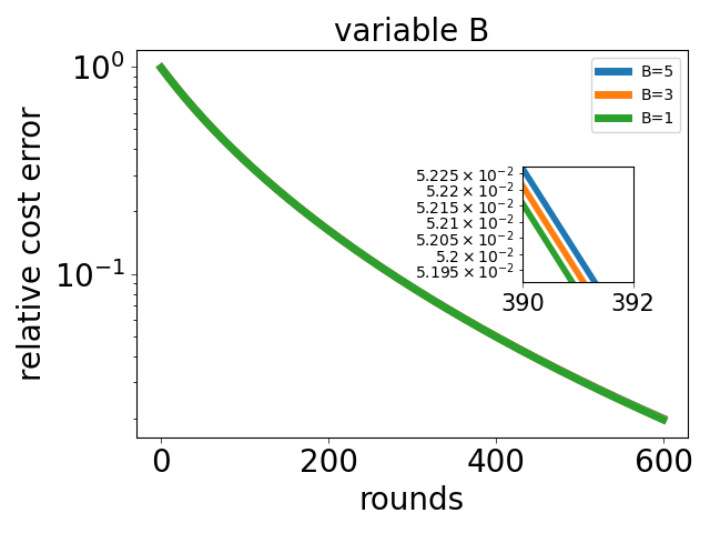
(b)

Figure 1: Computation cost to reach a target accuracy compared with [16] (a) and convergence paths for variable $B$ (b) (Full participation is considered in both cases).

(c)

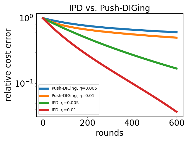
(d)

Figure 2: Comparison on different levels of participation for $B=5$ (a) and comparison (full participation) with Push-DIGing (b).

VII Conclusion

This paper proposed proposed IPD, a primal-dual method for distributed optimization over directed graphs. The two primal subproblems are solved inexactly: one step of gradient descent for the local optimization problem ($x-$variable) and distributed averaging based on weight balancing ($z-$variable). IPD was shown both theoretically and experimentally to have faster convergence than Push-DIGing (Sec. V) as well as substantial computation and communication savings over baseline methods. The established linear rate gives a decomposition in terms of the problem conditioning and the network connectivity (Thm. 1 and Cor. 1), similar with first order methods on undirected graphs. Furthermore, the lower bound for $B$ (number of communications per round) was shown to have a logarithmic dependency with conditioning and connectivity (Cor. 1). A distinctive attribute of IPD is the feasibility of partial agent participation, which is crucial in large-scale real systems (the rate was established in Thm. 2).

Appendix

Proof of Lemma 1: For each $k$, we consider the $l-$th entry of each $\xi_{i}^{k}\left(\cdot\right)$ and combine them to form an $n-$dimensional vector denoted by $\widetilde{\xi}^{k}\left(\cdot\right)$, and we let

$$\widetilde{\xi}^{k}_{\perp}\left(\cdot\right):=\left(I-\textbf{11}^{T}/n\right)\widetilde{\xi}^{k}\left(\cdot\right).$$

We define $W^{k}(b):=I-(D-A)\text{diag}\left(w^{k}(b)\right)$; this is column stochastic ($1^{T}W^{k}(b)=1^{T}$), which shows that $\xi^{k}(b+1)$ and $\xi^{k}(b)$ have the same sum (hence also average) since the update of the $l-$th entry can be written as:

$$\widetilde{\xi}^{k}\left(b+1\right)=W^{k}(b)\widetilde{\xi}^{k}\left(b\right).$$

The same reasoning also shows that $\bar{x}^{k}=\bar{z}^{k}$. Then, according to the first property of [16, Lemma 2], there exists $p^{k}(b)$, so that $W^{k}(b)p^{k}(b)=p^{k}(b)$ and $(p^{k}(b))^{T}\textbf{1}=1$. For any $b\in\{0,\ldots,B-1\}$, it follows from (6) that

$$\left(I-p^{k}(b)\textbf{1}^{T}\right)\left(\widetilde{\xi}^{k}(b+1)\right)$$

$$= \left(I-p^{k}(b)\textbf{1}^{T}\right)W^{k}(b)\widetilde{\xi}^{k}(b)$$

$$= \left(W^{k}(b)-p^{k}(b)\textbf{1}^{T}\right)\left(I-p^{k}(b)\textbf{1}^{T}\right)\widetilde{\xi}^{k}(b).$$

Additionally,

$$\left(I-p^{k}(b)\textbf{1}^{T}+\textbf{11}^{T}/n-\textbf{11}^{T}/n\right)\widetilde{\xi}^{k}(b+1)$$

$$= \left(W^{k}(b)-p^{k}(b)\textbf{1}^{T}\right)\left(I-p^{k}(b)\textbf{1}^{T}\right.$$

$$\left.+\textbf{11}^{T}/n-\textbf{11}^{T}/n\right)\widetilde{\xi}^{k}(b),$$

which implies

$$\widetilde{\xi}^{k}_{\perp}(b+1)+\left(\textbf{1}/n-p^{k}(b)\right)\textbf{1}^{T}\widetilde{\xi}^{k}(b+1)$$

$$= \left(W^{k}(b)-p^{k}(b)\textbf{1}^{T}\right)\left[\widetilde{\xi}^{k}_{\perp}(b)+(\textbf{1}/n-p^{k}(b))\textbf{1}^{T}\widetilde{\xi}^{k}(b)\right].$$

Then from the third property of [16, Lemma 2], for all $k\geq\bar{k}$

$$\norm{\widetilde{\xi}^{k}_{\perp}(b+1)+(\textbf{1}/n-p^{k}(b))\textbf{1}^{T}\widetilde{x}^{k}}\leq\delta\norm{\widetilde{\xi}^{k}_{\perp}(b)+(\textbf{1}/n-p^{k}(b))\textbf{1}^{T}\widetilde{x}^{k}}.$$

Iterating the inequality over $b=0$ to $b=B-1$, we obtain

$$\norm{\widetilde{z}^{k}_{\perp}+(\textbf{1}/n-p^{k}(B))\textbf{1}^{T}\widetilde{x}^{k}}\leq\delta^{B}\norm{\widetilde{x}^{k}_{\perp}+(\textbf{1}/n-p^{k}(0))\textbf{1}^{T}\widetilde{x}^{k}}.$$

Letting $\hat{p}^{k}=\arg\max_{p\in\{p^{k}(0),p^{k}(B)\}}\|1/n-p\|$, we get

$$\norm{\widetilde{z}^{k}_{\perp}} \leq\delta^{B}\norm{\widetilde{x}^{k}_{\perp}}+\left(1+\delta^{B}\right)\norm{(\textbf{1}/n-\hat{p}^{k})\textbf{1}^{T}\widetilde{x}^{k}}$$

$$\leq\delta^{B}\norm{\widetilde{x}^{k}_{\perp}}+2\norm{(\textbf{1}/n-\hat{p}^{k})\textbf{1}^{T}\widetilde{x}^{k}},$$

which implies (using $\delta\in(0,1),(a+b)^{2}\leq\frac{1}{\delta}a^{2}+\frac{1}{1-\delta}b^{2}$ for any $a,b\in\mathbb{R}$, along with Jensen’s inequality):

$$\norm{\widetilde{z}^{k}_{\perp}}^{2}\leq\delta^{2B-1}\norm{\widetilde{x}^{k}_{\perp}}^{2}+\frac{4}{1-\delta}\norm{(\textbf{1}/n-\hat{p}^{k})\textbf{1}^{T}\widetilde{x}^{k}}^{2}$$

$$= \delta^{2B-1}\norm{\widetilde{x}^{k}_{\perp}}^{2}$$

$$+\frac{4}{1-\delta}\norm{(\textbf{1}/n-\hat{p}^{k})\left(\textbf{1}^{T}\widetilde{x}^{k}-\textbf{1}^{T}\widetilde{x}^{\star}+\textbf{1}^{T}\widetilde{x}^{\star}\right)}^{2}$$

$$= \delta^{2B-1}\norm{\widetilde{x}^{k}_{\perp}}^{2}$$

$$+\frac{4}{1-\delta}\norm{\textbf{1}/n-\hat{p}^{k}}^{2}\left(\textbf{1}^{T}\widetilde{x}^{k}-\textbf{1}^{T}\widetilde{x}^{\star}+\textbf{1}^{T}\widetilde{x}^{\star}\right)^{2}$$

$$\leq \delta^{2B-1}\norm{\widetilde{x}^{k}_{\perp}}^{2}$$

$$+\frac{8}{1-\delta}\norm{\textbf{1}/n-\hat{p}^{k}}^{2}\left(\left(\textbf{1}^{T}\widetilde{x}^{k}-\textbf{1}^{T}\widetilde{x}^{\star}\right)^{2}+\left(\textbf{1}^{T}\widetilde{x}^{\star}\right)^{2}\right)$$

$$\leq \delta^{2B-1}\norm{\widetilde{x}^{k}_{\perp}}^{2}$$

$$+\frac{8}{1-\delta}\norm{\textbf{1}/n-\hat{p}^{k}}^{2}\left(n\norm{\widetilde{x}^{k}-\widetilde{x}^{\star}}^{2}+n\norm{\widetilde{x}^{\star}}^{2}\right)$$

Since $l$ is arbitrarily chosen from $\left\{1,\dots,d\right\}$, the inequality above holds for each entry position. Adding the $d$ inequalities together and defining $\Delta^{k}:=\frac{8n}{1-\delta}\norm{\textbf{1}/n-\hat{p}^{k}}^{2}$, which in view of the fact that both $\norm{\textbf{1}/n-p^{k}(0)}^{2}$ and $\norm{\textbf{1}/n-p^{k}(B)}^{2}$ tend to zero geometrically with the rate to be $\lambda_{2}(P)$ [20], completes the proof.$\hfill\blacksquare$

Proof of Theorem 1: For notational simplification, we denote $\nabla F\left(x^{k}\right)$ by $\nabla F^{k}$ and $\nabla F\left(x^{\star}\right)$ by $\nabla F^{\star}$. From (4) and (7c) we have

$$\nabla F^{k}-\nabla F^{\star}=-\frac{1}{\eta}(x^{k+1}-x^{k})-(y^{k}-y^{\star})-\rho(x^{k}-z^{k})$$

and

$$(x^{k}-x^{\star})^{T}(\nabla F^{k}-\nabla F^{\star})=$$

$$\underbrace{(x^{k+1}-x^{\star})^{T}(\nabla F^{k}-\nabla F^{\star})}_{(i)}+(x^{k}-x^{k+1})^{T}(\nabla F^{k}-\nabla F^{\star})$$

$(i)=\underbrace{-\frac{1}{\eta}(x^{k+1}-x^{\star})^{T}(x^{k+1}-x^{k})}_{(ii)}\\ \underbrace{-(x^{k+1}-x^{\star})^{T}(y^{k}-y^{\star})}_{(iii)}\underbrace{-\rho(x^{k+1}-x^{\star})^{T}(x^{k}-z^{k})}_{(iv)}$.
The following is to bound the three terms.

$$(ii)=\frac{1}{2\eta}\left(\norm{x^{k}-x^{\star}}^{2}-\norm{x^{k+1}-x^{\star}}^{2}-\norm{x^{k+1}-x^{k}}^{2}\right),$$

where we use parallelogram law

$$-2(a-b)^{T}(a-c)=\norm{b-c}^{2}-\norm{a-b}^{2}-\norm{a-c}^{2},$$

which is also used several times in the sequel.

$$(iii)=-(x^{k+1}-z^{k+1}+z^{k+1}-x^{\star})^{T}(y^{k}-y^{\star})$$

$$= -(x^{k+1}-z^{k+1})^{T}(y^{k}-y^{\star})-(z^{k+1}-x^{\star})^{T}(y^{k}-y^{\star})$$

$$\underset{(\ref{updatea})}{=} -\frac{1}{\rho}(y^{k+1}-y^{k})^{T}(y^{k}-y^{\star})-(z^{k+1}_{\perp})^{T}(y^{k}-y^{\star})$$

$$= -\frac{1}{2\rho}\left(\norm{y^{k+1}-y^{\star}}^{2}-\norm{y^{k}-y^{k+1}}^{2}-\norm{y^{k}-y^{\star}}^{2}\right)$$

$$-(z^{k+1}_{\perp})^{T}(y^{k}-y^{\star}),$$

where we use $z^{k+1}=\bar{x}^{k+1}+z^{k+1}_{\perp}$ and $\sum_{i=1}^{n}y_{i}^{k}=\sum_{i=1}^{n}y_{i}^{\star}=0$ from (7c).

$$(iv)=-\rho(x^{k+1}-x^{\star})^{T}(x^{k}-x^{k+1}+x^{k+1}-z^{k})$$

$$= -\rho(x^{k+1}-x^{\star})^{T}(x^{k+1}-z^{k})-\rho(x^{k+1}-x^{\star})^{T}(x^{k}-x^{k+1})$$

$$= \frac{\rho}{2}\left(\norm{x^{\star}-z^{k}}^{2}-\norm{x^{k+1}-x^{\star}}^{2}-\norm{x^{k+1}-z^{k}}^{2}\right)$$

$$-\frac{\rho}{2}\left(\norm{x^{\star}-x^{k}}^{2}-\norm{x^{k+1}-x^{\star}}^{2}-\norm{x^{k}-x^{k+1}}^{2}\right)$$

$$= \frac{\rho}{2}\left(\norm{x^{\star}-z^{k}}^{2}+\norm{x^{k}-x^{k+1}}^{2}-\norm{x^{\star}-x^{k}}^{2}\right.$$

$$\left.-\norm{x^{k+1}-z^{k}}^{2}\right).$$

Invoking Lemma 1 and using $\delta\in(0,1)$, we obtain:

$$\norm{x^{\star}-z^{k}}^{2}-\norm{x^{\star}-x^{k}}^{2}=\norm{z^{k}}^{2}-\norm{x^{k}}^{2}$$

$$= \norm{\bar{x}^{k}+z^{k}_{\perp}}^{2}-\norm{\bar{x}^{k}+x^{k}_{\perp}}^{2}$$

$$= \norm{\bar{x}^{k}}^{2}+\norm{z^{k}_{\perp}}^{2}+2\bar{x}^{kT}z^{k}_{\perp}-\norm{\bar{x}^{k}}^{2}-\norm{x^{k}_{\perp}}^{2}-2\bar{x}^{kT}x^{k}_{\perp}$$

$$= \norm{z^{k}_{\perp}}^{2}-\norm{x^{k}_{\perp}}^{2}+2\bar{x}^{kT}\left(z^{k}_{\perp}-x^{k}_{\perp}\right)$$

$$= \norm{z^{k}_{\perp}}^{2}-\norm{x^{k}_{\perp}}^{2}$$

$$\leq \left(\delta^{2B-1}-1\right)\norm{x^{k}_{\perp}}^{2}+\Delta^{k}\left(\norm{x^{k}-x^{\star}}^{2}+\norm{x^{\star}}^{2}\right)$$

$$\leq \Delta^{k}\left(\norm{x^{k}-x^{\star}}^{2}+\norm{x^{\star}}^{2}\right).$$

Adding the three terms together gives:

$$(i)\leq\frac{1}{2\eta}\left(\norm{x^{k}-x^{\star}}^{2}-\norm{x^{k+1}-x^{\star}}^{2}\right)$$

$$+\frac{1}{2\rho}\left(\norm{y^{k}-y^{\star}}^{2}-\norm{y^{k+1}-y^{\star}}^{2}\right)$$

$$+(\frac{\rho}{2}-\frac{1}{2\eta})\norm{x^{k+1}-x^{k}}^{2}+\frac{\rho}{2}\Delta^{k}\left(\norm{x^{k}-x^{\star}}^{2}+\norm{x^{\star}}^{2}\right)$$

$$\underbrace{+\frac{1}{2\rho}\norm{y^{k}-y^{k+1}}^{2}-\frac{\rho}{2}\norm{x^{k+1}-z^{k}}^{2}}_{(v)}\underbrace{\vphantom{\frac{1}{2\rho}}-(z^{k+1}_{\perp})^{T}(y^{k}-y^{\star})}_{(vi)}.$$

We proceed to bound $(v)$ and $(vi)$.
From (3c), $y^{k}-y^{k+1}=-\rho\left(x^{k+1}-z^{k+1}\right)$, so

$$(v)=\frac{\rho}{2}\left(\norm{x^{k+1}-z^{k+1}}^{2}-\norm{x^{k+1}-z^{k}}^{2}\right)$$

$$= \frac{\rho}{2}\left(\norm{x^{k+1}-\bar{x}^{k+1}-z^{k+1}_{\perp}}^{2}-\norm{x^{k+1}-\bar{x}^{k}-z^{k}_{\perp}}^{2}\right)$$

$$= \frac{\rho}{2}\left[\norm{x^{k+1}-\bar{x}^{k+1}}^{2}+\norm{z^{k+1}_{\perp}}^{2}-\norm{x^{k+1}-\bar{x}^{k}}^{2}-\norm{z^{k}_{\perp}}^{2}\right.$$

$$\left.-2(z^{k+1}_{\perp})^{T}(x^{k+1}-\bar{x}^{k+1})+2(z^{k}_{\perp})^{T}(x^{k+1}-\bar{x}^{k})\right]$$

$$\leq \frac{\rho}{2}\left[\norm{z^{k+1}_{\perp}}^{2}-2(z^{k+1}_{\perp})^{T}(x^{k+1}-\bar{x}^{k+1})\right.$$

$$\left.+2(z^{k}_{\perp})^{T}(x^{k+1}-\bar{x}^{k+1}+\bar{x}^{k+1}-\bar{x}^{k})\right]$$

$$\leq \frac{\rho}{2}\left[\norm{z^{k+1}_{\perp}}^{2}+\norm{z^{k+1}_{\perp}}^{2}+\norm{x^{k+1}_{\perp}}^{2}+2\norm{z^{k}_{\perp}}^{2}\right.$$

$$\left.+\norm{\bar{x}^{k+1}-\bar{x}^{k}}^{2}+\norm{x^{k+1}_{\perp}}^{2}\right]$$

$$\leq \frac{\rho}{2}\left\{(2\delta^{2B-1}+2)\norm{x^{k+1}_{\perp}}^{2}+2\delta^{2B-1}\norm{x^{k}_{\perp}}^{2}\right.$$

$$\left.+\norm{\bar{x}^{k+1}-\bar{x}^{k}}^{2}+2\Delta^{k}(\norm{x^{k}-x^{\star}}^{2}+\norm{x^{\star}}^{2})\right.$$

$$\left.+2\Delta^{k+1}(\norm{x^{k+1}-x^{\star}}^{2}+\norm{x^{\star}}^{2})\right\}.$$

From (4) and (7c),

$$y^{k}=-\frac{1}{\eta}(x^{k+1}-x^{k})-\nabla F^{k}-\rho(x^{k}-z^{k}),$$

$$(vi)=-(z^{k+1}_{\perp})^{T}\left[-\frac{1}{\eta}\left(x^{k+1}-x^{k}\right)-\left(\nabla F^{k}-\nabla F^{\star}\right)\right.$$

$$\left.\qquad\,\,\,\,-\rho\left(x^{k}-z^{k}\right)\right]$$

$$\leq \frac{\gamma}{4\eta}\left(\delta^{2B-1}\norm{x^{k+1}_{\perp}}^{2}+\Delta^{k+1}\left(\norm{x^{k+1}-x^{\star}}^{2}+\norm{x^{\star}}^{2}\right)\right)$$

$$+ \frac{1}{\gamma\eta}\norm{x^{k+1}-x^{k}}^{2}+\frac{1}{\zeta}\norm{\nabla F^{\star}-\nabla F^{k}}^{2}+\rho\norm{x^{k}-z^{k}}^{2}$$

$$+ \frac{\zeta}{4}\left(\delta^{2B-1}\norm{x^{k+1}_{\perp}}^{2}+\Delta^{k+1}\left(\norm{x^{k+1}-x^{\star}}^{2}+\norm{x^{\star}}^{2}\right)\right)$$

$$+ \frac{\rho}{4}\left(\delta^{2B-1}\norm{x^{k+1}_{\perp}}^{2}+\Delta^{k+1}\left(\norm{x^{k+1}-x^{\star}}^{2}+\norm{x^{\star}}^{2}\right)\right),$$

for arbitrary $\gamma,\zeta>0$. Note that $\norm{\bar{x}^{k+1}-\bar{x}^{k}}^{2}\leq\norm{x^{k+1}-x^{k}}^{2}$, and

$$\norm{x^{k}-z^{k}}^{2}=\norm{x^{k}_{\perp}-z^{k}_{\perp}}^{2}\leq 2\norm{x^{k}_{\perp}}^{2}+2\norm{z^{k}_{\perp}}^{2}$$

$$\leq (2+2\delta^{2B-1})\norm{x^{k}_{\perp}}^{2}+2\Delta^{k}\left(\norm{x^{k}-x^{\star}}^{2}+\norm{x^{\star}}^{2}\right).$$

For arbitrary $\tau>0$,

$$(\nabla F^{k}-\nabla F^{\star})^{T}(x^{k}-x^{k+1})\leq\tau\norm{x^{k}-x^{k+1}}^{2}+\frac{1}{4\tau}\norm{\nabla F^{k}-\nabla F^{\star}}^{2}.$$

Assumption 2 implies (cocoercivity of the gradient):

$$\left(x^{k}-x^{\star}\right)^{T}\left(\nabla F^{k}-\nabla F^{\star}\right)$$

$$\geq \frac{m_{f}M_{f}}{m_{f}+M_{f}}\norm{x^{k}-x^{\star}}^{2}+\frac{1}{m_{f}+M_{f}}\norm{\nabla F^{k}-\nabla F^{\star}}^{2}.$$

Putting everything together we obtain that for some $\widetilde{k}$ and all $k\geq\widetilde{k}$:

$$0\leq \left(\frac{1}{4\tau}+\frac{1}{\zeta}-\frac{1}{m_{f}+M_{f}}\right)\norm{\nabla F^{\star}-\nabla F^{k}}^{2}$$

$$+ \frac{1}{2\rho}\norm{y^{k}-y^{\star}}^{2}+\left(\tau+\rho+\frac{1}{\gamma\eta}-\frac{1}{2\eta}\right)\norm{x^{k}-x^{k+1}}^{2}$$

$$- \frac{1}{2\rho}\norm{y^{k+1}-y^{\star}}^{2}$$

$$+ \left\{\frac{1}{2\eta}+2\rho+3\rho\delta^{2B-1}-\frac{m_{f}M_{f}}{m_{f}+M_{f}}\right\}\norm{x^{k}-x^{\star}}^{2}$$

$$- \left\{\frac{1}{2\eta}-\delta^{2B-1}\left[\frac{5\rho}{4}+\frac{\gamma}{4\eta}+\frac{\zeta}{4}\right]-\rho\right\}\norm{x^{k+1}-x^{\star}}^{2}$$

$$+ \frac{7\rho}{2}\Delta^{k}\left(\norm{x^{k}-x^{\star}}^{2}+\norm{x^{\star}}^{2}\right)$$

$$+ \left(\frac{\gamma}{4\eta}+\frac{\zeta}{4}+\frac{5\rho}{4}\right)\Delta^{k+1}\left(\norm{x^{k+1}-x^{\star}}^{2}+\norm{x^{\star}}^{2}\right).$$

By applying Jensen’s inequality and (4) along with the previously obtained bound on $\|x^{k}-z^{k}\|$,

$$\frac{1}{3}\norm{y^{k}-y^{\star}}^{2}\leq \frac{1}{\eta^{2}}\norm{x^{k+1}-x^{k}}^{2}+\norm{\nabla F^{\star}-\nabla F^{k}}^{2}$$

$$+\rho^{2}(2+2\delta^{2B-1})\norm{x^{k}-x^{\star}}^{2}$$

$$+2\rho^{2}\Delta^{k}\left(\norm{x^{k}-x^{\star}}^{2}+\norm{x^{\star}}^{2}\right).$$

It thus all boils down to choosing suitable $B,\eta,\tau,\zeta$, such that the following inequalities hold:

$$\frac{1}{4\tau}+\frac{1}{\zeta}-\frac{1}{m_{f}+M_{f}}<0,$$ (12a)

$$\tau+\rho+\frac{1}{\gamma\eta}-\frac{1}{2\eta}<0,$$ (12b)

$$\frac{1}{2\eta}-\left[\delta^{2B-1}\left(\frac{5\rho}{4}+\frac{\gamma}{4\eta}+\frac{\zeta}{4}\right)+\rho\right]>0,$$ (12c)

$$\delta^{2B-1}\left(\frac{17\rho}{4}+\frac{\gamma}{4\eta}+\frac{\zeta}{4}\right)+3\rho-\frac{m_{f}M_{f}}{m_{f}+M_{f}}<0.$$ (12d)

By choosing $\gamma=4,\tau=\frac{3(M_{f}+m_{f})}{4},\eta\leq\frac{4}{15(M_{f}+m_{f})},\zeta=3(M_{f}+m_{f})$, there exist $\mu_{1},\mu_{2},\mu_{3},k_{1}$, such that $0<\mu_{1}<\mu_{2}$ and for all $k>k_{1}$, the following holds:

$$\mu_{1}\left(\norm{x^{k}-x^{\star}}^{2}+\norm{y^{k}-y^{\star}}^{2}\right)+\mu_{3}\left(\Delta^{k}+\Delta^{k+1}\right)\norm{x^{\star}}^{2}$$

$$\geq\norm{x^{k+1}-x^{\star}}^{2}+\norm{y^{k+1}-y^{\star}}^{2}$$

where $\mu_{1}=\max\left\{\frac{c_{1}+c_{2}}{2c_{2}},\left(\frac{1}{2\rho}-c_{3}\right)/\left(\frac{1}{2\rho}\right)\right\}$ and $c_{1},c_{2},c_{3}$ are specified in the statement of the theorem.
Denoting $\omega^{k}:=\mu_{3}\left(\Delta^{k}+\Delta^{k+1}\right)\norm{x^{\star}}^{2}$, we have established

$$\mu_{1}\left(\norm{x^{k}-x^{\star}}^{2}+\norm{y^{k}-y^{\star}}^{2}\right)+\omega^{k}$$

$$\geq \norm{x^{k+1}-x^{\star}}^{2}+\norm{y^{k+1}-y^{\star}}^{2},$$

and $\omega^{k}$ tends to zero geometrically with rate $\lambda_{2}(P)$. We consider two cases:
$\bullet$ if there exists a subsequence $k_{(l)}$ such that

$$\frac{1-\mu_{1}}{2}\left(\norm{x^{k_{(l)}+1}-x^{\star}}^{2}+\norm{y^{k_{(l)}+1}-y^{\star}}^{2}\right)<\omega^{k_{(l)}},$$ (13)

then the subsequence $\norm{x^{k_{(l)}+1}-x^{\star}}^{2}+\norm{y^{k_{(l)}+1}-y^{\star}}^{2}\rightarrow 0$ geometrically with rate $\lambda_{2}(P)$ and hence also $\lambda$. For $k$ that does not satisfy (13), we have

$$\mu_{1}\left(\norm{x^{k}-x^{\star}}^{2}+\norm{y^{k}-y^{\star}}^{2}\right)$$

$$\geq \frac{1+\mu_{1}}{2}\left(\norm{x^{k+1}-x^{\star}}^{2}+\norm{y^{k+1}-y^{\star}}^{2}\right),$$ (14)

so again this shows asymptotic rate $\lambda$.
$\bullet$ if there exists some $k_{2}$ so that for all $k\geq k_{2}$, the reverse of (13) holds, then for all $k$, (14) holds.
We conclude that in both cases, $\norm{x^{k}-x^{\star}}^{2}+\norm{y^{k}-y^{\star}}^{2}\rightarrow 0$ geometrically with rate $\lambda$.$\hfill\blacksquare$

Proof of Theorem 2: Let $\Omega^{k}\in\mathbb{R}^{n\times n}$ be a $0-1$ diagonal matrix where $1$ corresponds to the case agent $i$ is active and $0$ when it is inactive. Let $\mathbb{E}\left[\Omega^{k}\right]=\Omega:=\text{diag}(q_{1},\ldots,q_{n})$.
The update of $w$ can be written compactly as

$$w^{k}(b+1)=w^{k}(b)+\Omega^{k}\left(Pw^{k}(b)-w^{k}(b)\right).$$

Let $w^{\infty}=\underset{t\rightarrow\infty}{\text{lim}}P^{t}w^{0}(0)$, then we have

$$\norm{w^{k}(b+1)-w^{\infty}}^{2}_{\Omega^{-1}}$$

$$= \norm{w^{k}(b)+\Omega^{k}\left(Pw^{k}(b)-w^{k}(b)\right)-w^{\infty}}^{2}_{\Omega^{-1}}$$

$$= \norm{w^{k}(b)-w^{\infty}}^{2}_{\Omega^{-1}}$$

$$+\left(Pw^{k}(b)-w^{k}(b)\right)^{T}\Omega^{k}\Omega^{-1}\Omega^{k}\left(Pw^{k}(b)-w^{k}(b)\right)$$

$$+2\left(w^{k}(b)-w^{\infty}\right)^{T}\Omega^{-1}\left(\Omega^{k}\left(Pw^{k}(b)-w^{k}(b)\right)\right)$$

$$= \norm{w^{k}(b)-w^{\infty}}^{2}_{\Omega^{-1}}$$

$$+\left(Pw^{k}(b)-w^{k}(b)\right)^{T}\Omega^{-1}\Omega^{k}\left(Pw^{k}(b)-w^{k}(b)\right)$$

$$+2\left(w^{k}(b)-w^{\infty}\right)^{T}\Omega^{-1}\left(\Omega^{k}\left(Pw^{k}(b)-w^{k}(b)\right)\right),$$

where we have used idempotency of $\Omega^{k}$ (as 0-1 diagonal matrix) and the fact that diagonal matrices commute. By taking conditional expectation (denoted by $\mathbb{E}^{k}$, where conditioning is on past activations) on both sides, we have

$$\mathbb{E}^{k}\left[\norm{w^{k}(b+1)-w^{\infty}}^{2}_{\Omega^{-1}}\right]$$

$$= \norm{w^{k}(b)-w^{\infty}}^{2}_{\Omega^{-1}}+\norm{Pw^{k}(b)-w^{k}(b)}^{2}$$

$$+2\left(w^{k}(b)-w^{\infty}\right)^{T}\left(Pw^{k}(b)-w^{k}(b)\right).$$

From [20, Lemma 1], there exists some positive $\theta<1$ only depending on $P$, such that

$$\norm{Pw^{k}(b)-w^{k}(b)}^{2}+2\left(w^{k}(b)-w^{\infty}\right)^{T}\left(Pw^{k}(b)-w^{k}(b)\right)$$

$$\leq-\theta\norm{w^{k}(b)-w^{\infty}}^{2},$$

which implies

$$\mathbb{E}^{k}\left[\norm{w^{k}(b+1)-w^{\infty}}^{2}_{\Omega^{-1}}\right]\leq\left(1-q_{\text{min}}\theta\right)\norm{w^{k}(b)-w^{\infty}}^{2}_{\Omega^{-1}}.$$

By induction, we obtain

$$\mathbb{E}\left[\norm{w^{k}(b)-w^{\infty}}^{2}\right]\leq c_{1}\lambda^{kB+b}_{2}$$

for some constant $c_{1}$ and $\lambda_{2}:=1-q_{\text{min}}\theta$, whence invoking Markov’s inequality for arbitrary $\epsilon_{1}>0$ gives

$$\text{Pr}\left[\norm{w^{k}(b)-w^{\infty}}^{2}\geq\epsilon_{1}\right]\leq\frac{1}{\epsilon_{1}}c_{1}\lambda_{2}^{kB+b}.$$

This further implies

$$\underset{n\rightarrow\infty}{\text{lim}}\text{Pr}\left[\cup^{\infty}_{k=n}\cup^{B-1}_{b=0}\left\{\norm{w^{k}(b)-w^{\infty}}^{2}>\epsilon_{1}\right\}\right]=0,$$

i.e., $\forall\epsilon>0$, $\exists K_{1}(\epsilon)$, such that

$$\text{Pr}\left[\cup^{\infty}_{k=K_{1}}\cup^{B-1}_{b=0}\left\{\norm{w^{k}(b)-w^{\infty}}^{2}>\epsilon_{1}\right\}\right]\leq\frac{\epsilon}{2},$$

which implies

$$\text{Pr}\left[\cap^{\infty}_{k=K_{1}}\cap^{B-1}_{b=0}\left\{\norm{w^{k}(b)-w^{\infty}}^{2}<\epsilon_{1}\right\}\right]\geq 1-\frac{\epsilon}{2}.$$ (15)

We define $v^{k}:=\left[(x^{k})^{T},(y^{k})^{T}\right]^{T}$, and let $T_{a}$ to be the operator corresponding to Alg. 1 for full participation, i.e., $T_{a}:(x^{k},y^{k},z^{k})\mapsto(x^{k+1},y^{k+1},z^{k+1})$ and $T:=\begin{bmatrix}I_{d}\quad 0\quad 0\\ 0\,\quad I_{d}\quad 0\end{bmatrix}T_{a}$.
We define $\Phi^{k}:=\text{blkdiag}\left(\Omega^{k}\otimes I_{d},\Omega^{k}\otimes I_{d}\right)$ and $\Phi^{k}_{a}:=\text{blkdiag}\left(\Omega^{k}\otimes I_{d},\Omega^{k}\otimes I_{d},\Omega^{k}\otimes I_{d}\right)$, then
$\mathbb{E}\left[\Phi^{k}\right]=\Phi:=\text{blkdiag}\left(\Omega\otimes I_{d},\Omega\otimes I_{d}\right)$ and we have

$\Phi^{k}T=\Phi^{k}\begin{bmatrix}I_{d}\quad 0\quad 0\\ 0\,\quad I_{d}\quad 0\end{bmatrix}T_{a}=\begin{bmatrix}I_{d}\quad 0\quad 0\\ 0\,\quad I_{d}\quad 0\end{bmatrix}\Phi_{a}^{k}T_{a}$,

which allows the analysis to carry for $T$ only.
For partial participation, we have

$$v^{k+1}=v^{k}+\Phi^{k}\left(Tv^{k}-v^{k}\right),$$

i.e.,

$$\norm{v^{k+1}-v^{\star}}^{2}_{\Phi^{-1}}=\norm{v^{k}-v^{\star}+\Phi^{k}\left(Tv^{k}-v^{k}\right)}^{2}_{\Phi^{-1}}.$$

There are two possibilities (depending on whether (13) is satisfied) either

$$\norm{Tv^{k}-v^{\star}}^{2}\leq\frac{2\mu_{1}}{\mu_{1}+1}\norm{v^{k}-v^{\star}}^{2}$$

or

$$\norm{Tv^{k}-v^{\star}}^{2}\leq\frac{2}{1-\mu_{1}}\omega^{k},$$

where $\omega^{k}\rightarrow 0$. For the first case we have

$$\mathbb{E}^{k}\left[\norm{v^{k+1}-v^{\star}}^{2}_{\Phi^{-1}}\right]\leq\left(1-(1-\frac{2\mu_{1}}{\mu_{1}+1})q_{\min}\right)\norm{v^{k}-v^{\star}}^{2}_{\Phi^{-1}}.$$

For the second we have

$$\norm{v^{k+1}-v^{\star}}^{2}_{\Phi^{-1}}=\norm{v^{k}-v^{\star}+\Phi^{k}\left(Tv^{k}-v^{k}\right)}^{2}_{\Phi^{-1}}$$

$$= \norm{\Phi^{k}(Tv^{k}-v^{\star})+(I-\Phi^{k})(v^{k}-v^{\star})}^{2}_{\Phi^{-1}}$$

$$\leq \frac{1}{\beta}\norm{\Phi^{k}(Tv^{k}-v^{\star})}^{2}_{\Phi^{-1}}+\frac{1}{1-\beta}\norm{(I-\Phi^{k})(v^{k}-v^{\star})}^{2}_{\Phi^{-1}},$$

taking expectation and noting that

$$\mathbb{E}\left[\norm{(I-\Phi^{k})(v^{k}-v^{\star})}^{2}_{\Phi^{-1}}\right]\leq(1-q_{\min})^{2}\norm{v^{k}-v^{\star}}^{2}_{\Phi^{-1}},$$

implies that

$$\mathbb{E}^{k}\left[\norm{v^{k+1}-v^{\star}}^{2}_{\Phi^{-1}}\right]\leq\frac{1}{\beta}\omega^{k}+\frac{(1-q_{\min})^{2}}{1-\beta}\norm{v^{k}-v^{\star}}^{2}_{\Phi^{-1}},$$

for any $\beta>0$, whence choosing $\beta=q_{\min}$, we obtain

$$\mathbb{E}^{k}\left[\norm{v^{k+1}-v^{\star}}^{2}_{\Phi^{-1}}\right]\leq\frac{1}{q_{\min}}\omega^{k}+(1-q_{\min})\norm{v^{k}-v^{\star}}^{2}_{\Phi^{-1}}.$$

By induction, we conclude that for both cases

$$\mathbb{E}\left[\norm{v^{k+1}-v^{\star}}^{2}_{\Phi^{-1}}\right]\leq c_{2}\lambda_{1}^{k},$$

where $\lambda_{1}$ is as Thm. 2 states.
An analogous use of Markov’s inequality in the establishment of (15) concludes there exists some $K_{2}$, such that

$$\text{Pr}\left[\cap_{k=K_{2}}^{\infty}\norm{v^{k+1}-v^{\star}}^{2}_{\Phi^{-1}}\leq\lambda_{p}^{k}\right]\geq 1-\frac{\epsilon}{2},$$

where $\lambda_{p}$ can be arbitrarily chosen from $\left(\lambda_{1},1\right)$, and hence finishes the proof.$\hfill\blacksquare$

References

• [1] A. Nedić and J. Liu, “Distributed optimization for control,” Annual Review of Control, Robotics, and Autonomous Systems, vol. 1, pp. 77–103, 2018.
• [2] A. Dimakis, S. Kar, J. Moura, M. Rabbat, and A. Scaglione, “Gossip algorithms for distributed signal processing,” Proceedings of the IEEE, vol. 98, no. 11, pp. 1847–1864, 2010.
• [3] P. Sopasakis, N. M. Freris, and P. Patrinos, “Accelerated reconstruction of a compressively sampled data stream,” in IEEE European Signal Processing Conference (EUSIPCO), 2016, pp. 1078–1082.
• [4] J. Verbraeken, M. Wolting, J. Katzy, J. Kloppenburg, T. Verbelen, and J. S. Rellermeyer, “A survey on distributed machine learning,” ACM computing surveys (csur), vol. 53, no. 2, pp. 1–33, 2020.
• [5] M. Vlachos, N. M. Freris, and A. Kyrillidis, “Compressive mining: fast and optimal data mining in the compressed domain,” The VLDB Journal, vol. 24, no. 1, pp. 1–24, 2015.
• [6] N. M. Freris, H. Kowshik, and P. R. Kumar, “Fundamentals of large sensor networks: Connectivity, capacity, clocks, and computation,” Proceedings of the IEEE, pp. 1828–1846, 2010.
• [7] C. Intanagonwiwat, R. Govindan, D. Estrin, J. Heidemann, and F. Silva, “Directed diffusion for wireless sensor networking,” IEEE/ACM Transactions on Networking, vol. 11, no. 1, pp. 2–16, 2003.
• [8] A. Nedic and A. Ozdaglar, “Distributed subgradient methods for multi-agent optimization,” IEEE Transactions on Automatic Control, vol. 54, pp. 48–61, 2009.
• [9] A. Makhdoumi and A. Ozdaglar, “Convergence rate of distributed ADMM over networks,” IEEE Transactions on Automatic Control, vol. 62, no. 10, pp. 5082–5095, 2017.
• [10] T. H. Chang, M. Hong, and X. Wang, “Multi-agent distributed optimization via inexact consensus ADMM,” IEEE Transactions on Signal Processing, vol. 63, no. 2, pp. 482–497, 2014.
• [11] N. S. Aybat, Z. Wang, T. Lin, and S. Ma, “Distributed linearized alternating direction method of multipliers for composite convex consensus optimization,” IEEE Transactions on Automatic Control, vol. 63, no. 1, pp. 5–20, 2018.
• [12] S. Boyd, N. Parikh, E. Chu, B. Peleato, and J. Eckstein, “Distributed optimization and statistical learning via the alternating direction method of multipliers,” Foundations and Trends® in Machine Learning, vol. 3, no. 1, pp. 1–122, 2011.
• [13] A. Nedić and A. Olshevsky, “Distributed optimization over time-varying directed graphs,” IEEE Transactions on Automatic Control, vol. 60, no. 3, pp. 601–615, 2014.
• [14] A. Nedić and A. Olshevsky, “Stochastic gradient-push for strongly convex functions on time-varying directed graphs,” IEEE Transactions on Automatic Control, vol. 61, no. 12, pp. 3936–3947, 2016.
• [15] A. Nedić, A. Olshevsky, and W. Shi, “Achieving geometric convergence for distributed optimization over time-varying graphs,” SIAM Journal on Optimization, vol. 27, no. 4, pp. 2597–2633, 2017.
• [16] K. Rokade and R. K. Kalaimani, “Distributed ADMM over directed networks,” arXiv e-prints, arXiv:2010.10421, 2020.
• [17] W. Jiang, A. Grammenos, E. Kalyvianaki, and T. Charalambous, “An asynchronous approximate distributed alternating direction method of multipliers in digraphs,” in IEEE Conference on Decision and Control (CDC), 2021, pp. 3406–3413.
• [18] V. Khatana and M. V. Salapaka, “DC-DistADMM: ADMM algorithm for contsrained distributed optimization over directed graphs,” arXiv preprint, arXiv:2003.13742, 2020.
• [19] N. M. Freris, S. R. Graham, and P. R. Kumar, “Fundamental limits on synchronizing clocks over networks,” IEEE Transactions on Automatic Control, vol. 56, no. 6, pp. 1352–1364, 2010.
• [20] A. Makhdoumi and A. Ozdaglar, “Graph balancing for distributed subgradient methods over directed graphs,” in IEEE Conference on Decision and Control (CDC), 2015, pp. 1364–1371.