Deep Gaussian Process-based Multi-fidelity Bayesian Optimization for Simulated Chemical Reactors

Abstract

New manufacturing techniques such as 3D printing have recently enabled the creation of previously infeasible chemical reactor designs. Optimizing the geometry of the next generation of chemical reactors is important to understand the underlying physics and to ensure reactor feasibility in the real world. This optimization problem is computationally expensive, nonlinear, and derivative-free making it challenging to solve. In this work, we apply deep Gaussian processes (DGPs) to model multi-fidelity coiled-tube reactor simulations in a Bayesian optimization setting. By applying a multi-fidelity Bayesian optimization method, the search space of reactor geometries is explored through an amalgam of different fidelity simulations which are chosen based on prediction uncertainty and simulation cost, maximizing the use of computational budget. The use of DGPs provides an end-to-end model for five discrete mesh fidelities, enabling less computational effort to gain good solutions during optimization. The accuracy of simulations for these five fidelities is determined against experimental data obtained from a 3D printed reactor configuration, providing insights into appropriate hyper-parameters. We hope this work provides interesting insight into the practical use of DGP-based multi-fidelity Bayesian optimization for engineering discovery.

1 Introduction

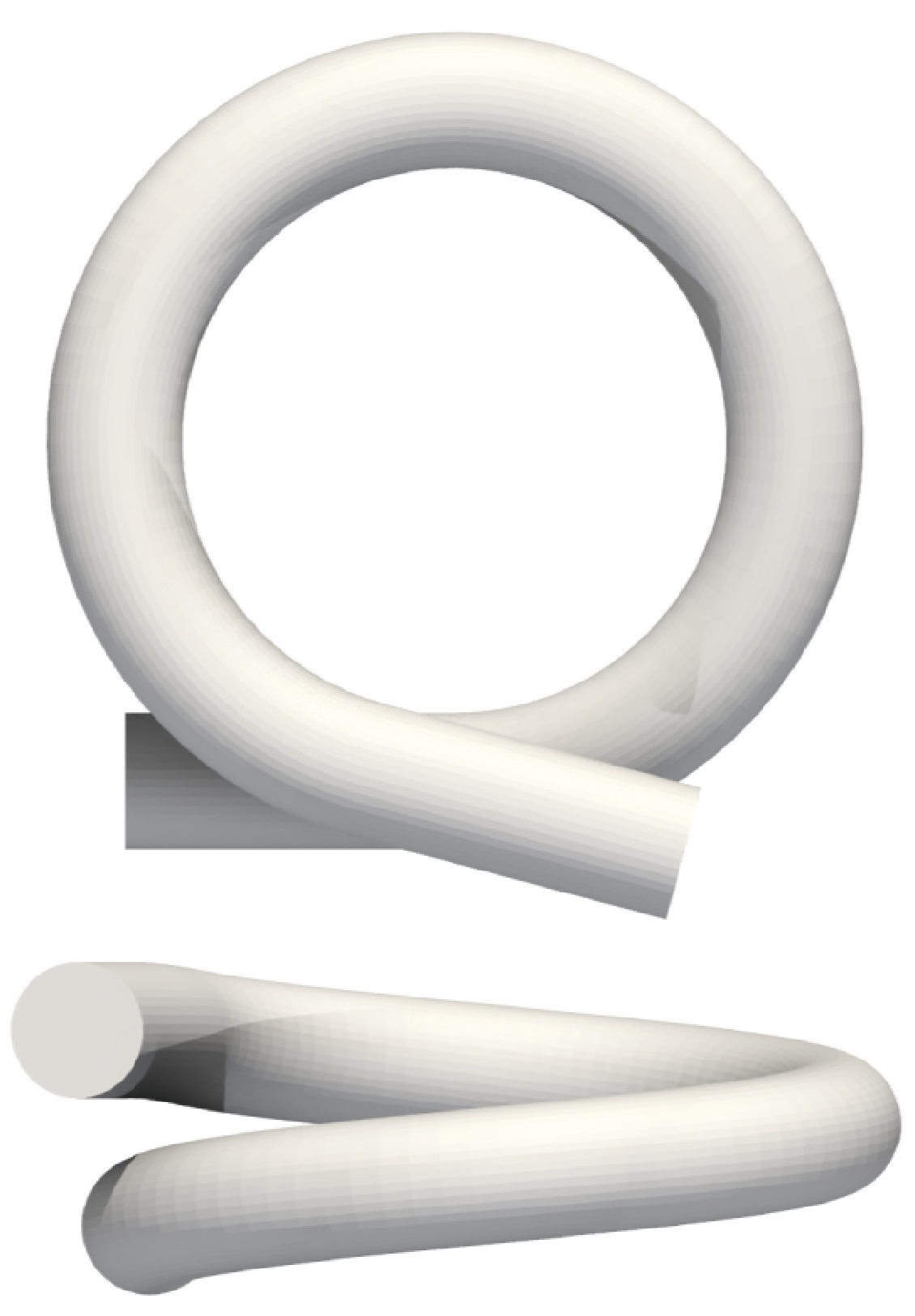
The fluid flow within a reactor greatly influences product quality and is highly dependent on the reactor geometry. Plug-flow conditions, corresponding to a product distributions with low variance, are desired. We study coiled tube reactors, which have been shown to demonstrate promising plug flow performance in previous computational and experimental studies [13, 12, 17, 16, 4].

Computational fluid dynamics (CFD) simulations of coiled-tube reactors are expensive due to complex flow characteristics, and gradient information is practically unavailable. The resulting expensive black-box optimization problem is analogous to hyper-parameter optimization [23, 10, 5, 1], with chemical discovery [7, 15], and engineering design [9, 18, 3] also examples of domains where expensive black-box optimization problems are formulated. The problem can be stated as

$$x^{*}=\mathop{\mathrm{argmax}}_{x\in\mathcal{X}\subset\mathbb{R}^{d}}f(x).$$ (1)

In certain situations, computational expense can be traded off with accuracy via one or multiple fidelity parameters. Examples include training epochs [22, 21] in the context of hyper-parameter optimization, mesh fidelities in the context of finite element analysis [6], or combining real-time measurements and predictions in industrial processes [20]. Including fidelity control within a Bayesian optimization framework enables optimization with fewer computational resources whilst gaining a ‘high fidelity’ solution [11, 14]. Equation 1 then becomes

$$x^{*}=\mathop{\mathrm{argmax}}_{x\in\mathcal{X}\subset\mathbb{R}^{d}}f(x,s)$$ (2)

where potentially M different fidelities, $s\in\mathbb{R}^{M}$ become controllable parameters.

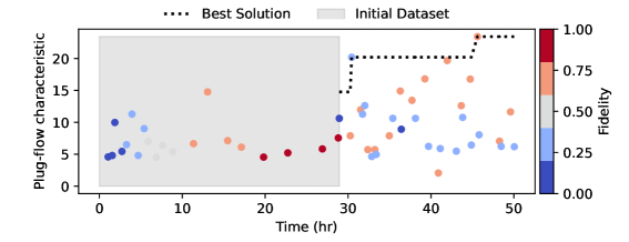
Contribution: In this work, we present the novel real-world problem of optimizing the geometry of a coiled tube reactor to maximize the plug-flow performance. We apply a state-of-the-art deep GP-based multi-fidelity Bayesian optimization algorithm to identify novel reactor configurations using an amalgam of different fidelity simulations, modeled using a DGP. Figure 1 demonstrates how our approach takes advantage of lower fidelity simulations. Our approach contains no additional hyper-parameters when compared to standard UCB Bayesian optimization. Having identified an optimal geometry we investigate the physical insights to inform future design of pulsed-flow coiled tube reactors.

Figure 1: Left: The progression of multi-fidelity Bayesian optimization using DGPs as a multi-fidelity model. Multiple different fidelity levels are selected for evaluation throughout optimization, reducing optimization time. Right: the best coil geometry which has a relatively large coil radius and low pitch.

2 Method

By applying DGPs within a Bayesian optimization framework, we enable an end-to-end model of all fidelities. A more accurate model of higher-fidelities should enable the optimization procedure to make more evaluations at lower, less expensive fidelities.

2.1 Model fidelities

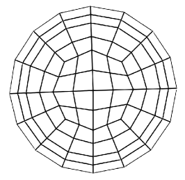
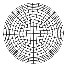
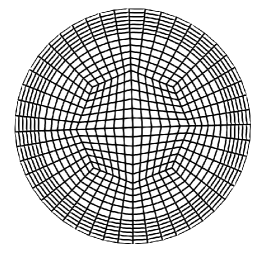
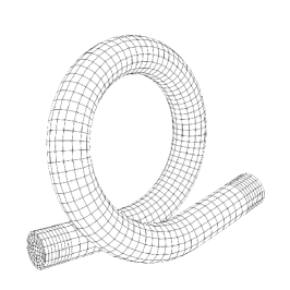
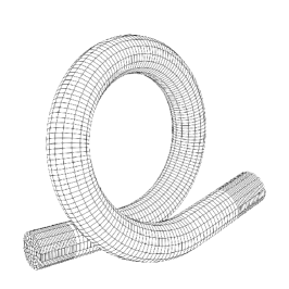
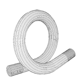
Two fidelity aspects, axial and radial, can be varied when meshing is performed given a tube geometry. Figure 2 demonstrates how axial and radial fidelity effects the final mesh. In this work, we combine both aspects into a single fidelity, and identify five discrete fidelity values. We leave the case in which axial and radial fidelities are allowed to vary independently for future work.

(a) Left: Radial cross section depicting radial fidelity at values of 0, 0.5 and 1.

(b) Right: View of complete reactor at axial fidelity values of 0, 0.5, and 1.

Figure 2: An instance of coiled tube reactor geometry as effected by axial and radial fidelity.

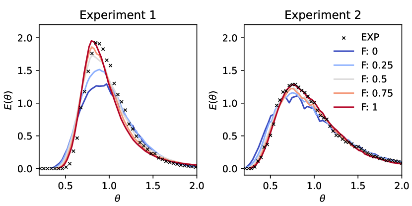
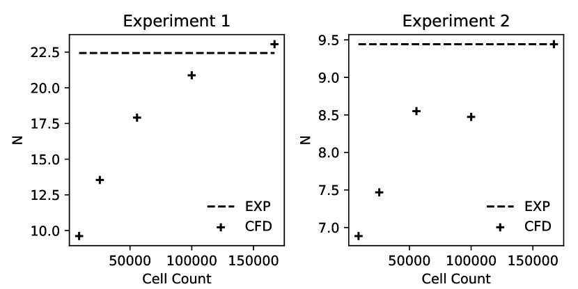
To investigate the effect of fidelity on function accuracy, the five discrete fidelities were simulated and compared with experimental data. Figure 3 validates the tracer concentration profile of simulations using the five fidelities against two sets of experimental data. The objective of the optimization is to maximize the plug-flow characteristic $N$ (high values of $N$ are an indicator for good radial mixing and poor axial mixing), which approximately corresponds to fitting the concentration profile with the tank-in-series model [16]. Figure 3 also demonstrates how increasing fidelity (and therefore cell count) results in a closer approximation to the experimental value of $N$, derived from each concentration profile.

(a) Left: The concentration profile of a tracer injection at five fidelity levels between 0 and 1 against experimentally obtained data. $E(\theta)$ represents dimensionless concentration as a function of dimensionless time $\theta$.

(b) Right: The value of N corresponding to the concentration profile from each fidelity, which has been converted to cell count. N represents plug-flow characteristic which is the quantity optimized for.

Figure 3: Validation of five discrete mesh fidelities corresponding to different cell counts, across two sets of experimental data under different conditions.

2.2 Model specification

To model each fidelity level we apply Deep Gaussian processes as demonstrated by Cutajar et al. [2]. DGPs provide a natural extension to sequentially trained multi-fidelity models, where a generating function $f$ at a given discrete fidelity $t$ is modeled as a linear or nonlinear function of lower-fidelities plus a mismatch term. For example in the nonlinear case $f_{t}(x)$ is given by

$$f_{t}(x)=\rho_{t-1}(f_{t-1}(x),x)+\phi_{t-1}(x).$$ (3)

Multi-fidelity DGPs combine $\rho_{t-1}$ and $\phi_{t-1}$ into a single term $g_{t-1}$ which is modeled using a GP, resulting in a composition of GPs. For example for $t$ different fidelity levels, and observations $x$ at each fidelity, the highest fidelity is modeled as

$$f_{t}(x_{t},\dots,x_{1})=g_{t}(...g_{t-1}(g_{1}(x_{1}),x_{t-1}),x_{t}).$$ (4)

In this work, we assume five discrete fidelity levels. Thus the resulting DGP has five layers ($t=5$), corresponding to simulations at fidelities equal to 0, 0.25, 0.5, 0.75, and 1. MF-DGPs are implemented in Python using emukit [19].

2.3 Multi-fidelity Bayesian Optimization

We present an approach for multi-fidelity Bayesian optimisation inspired by the MF-GP-UCB algorithm [8]. We find that the number of hyper-parameters in MF-GP-UCB is generally unsustainable for a problem with no prior knowledge, and a large number of fidelities. Algorithm 1 demonstrates the simplified approach we apply, inspired by MF-GP-UCB. The two main differences being the use of DGPs to model relationships between fidelities as opposed to separate models, and a simplified fidelity selection which is directly tied to the computational expense of an evaluation at a given fidelity. The approach differs from standard UCB-BO by including an additional discrete sub-problem to select the subsequent simulation fidelity, based on uncertainty and computational expense at each fidelity.

Algorithm 1 Deep GP-based Multi-fidelity Bayesian Optimization

0:  $f_{1}(x)\dots f_{T}(x)$, $\mathcal{X}$, $n$

  for $t$ in $1,\dots,T$ do

     Generate $n$ samples, $\mathbf{x}_{t}$, and evaluate $f_{t}(\mathbf{x})$ resulting in $\mathbf{y}_{t}$.

     $\tau_{t}\leftarrow$ average simulation time

  end for

  while Budget not exhausted do

     Train DGP using $\mathbf{x}_{1},\dots,\mathbf{x}_{T}$ and $\mathbf{y}_{1},\dots,\mathbf{y}_{T}$

     Solve UCB for highest-fidelity: $x^{*}\leftarrow\arg\max_{x}\{\mu_{T}(x)+\beta^{1/2}\sigma_{T}(x)|x\in\mathcal{X}\}$

     Choose fidelity based on variance of DGP and simulation cost: $t^{*}\leftarrow\text{argmax}_{t}\{\gamma_{t}\beta^{1/2}\sigma_{t}(x^{*})\}$ where $\gamma_{t}=\max(\tau)/\tau_{t}$

     Evaluate $f_{t^{*}}(x^{*})$, add $x^{*}$ to $\mathbf{x}_{t^{*}}$ and $f_{t^{*}}(x^{*})$ to $\mathbf{y}_{t^{*}}$

  end while

We note that in choosing $\gamma_{t}$ based on the points sampled to construct the initial DGP, the algorithm contains no additional hyper-parameters than standard UCB Bayesian optimization. Additionally $\gamma_{t}$ may be updated after a simulation has been performed, more accurately reflecting the simulation time at that fidelity.

3 Experimental results

Figure 1 demonstrates the MF-DGP based optimization, which shows the selection of multiple simulation fidelities throughout optimization.

We note that initializing the DGPs for multi-fidelity modeling requires simulations at each fidelity. As Bayesian optimization typically demonstrates fast early convergence, this provides a downside over the standard single fidelity approach, as more time is used to generate the initial data set.

3.1 Recommendations

Overall we find that it may not be beneficial in situations where a large number of discrete fidelities are available, to apply all fidelities within an optimization framework. A large number of fidelities results in a large number of hyper-parameters, more difficult to train multi-fidelity models such as DGPs with more layers resulting in longer inference times, and potentially slower exploration. We make the recommendation to apply 2 or 3 discrete fidelities in systems with no prior knowledge, despite more being available. Future work will compare the multi-fidelity approaches with varying number of fidelities with standard approaches and investigate the benefits, as well as apply similar methods on more, industrial case studies for engineering discovery.

4 Conclusions

The optimization of coiled tube reactor geometry is critical to maximize plug-flow behavior and investigate industrial viability. The optimization problem is formulated as an expensive black-box problem. In this paper, we propose multi-fidelity Bayesian optimization using Deep Gaussian processes to find good reactor configurations, taking advantage of less accurate but faster simulations. We demonstrate experimental validation of five discrete fidelities, and present a modified multi-fidelity Bayesian optimization algorithm which relies on fewer hyper-parameters than existing approaches. A multi-fidelity DGP provides correct quantification and propagation of uncertainty, which we use to select not only the next experimental design, but also the fidelity of the evaluation within the algorithm. Our approach can be extended to other problems involving parameterized CFD simulations. This work demonstrates an industrially relevant use case of multi-fidelity deep Gaussian processes for the optimization of expensive black-box functions. We hope it provides insight and inspiration for people in the machine learning community to develop methods for a variety of applied case-studies and problems.

Appendix A Simulation time at each fidelity

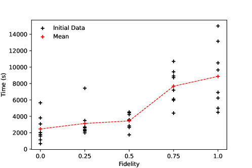
To dictate hyper-parameters $\gamma$ at each fidelity, weighting the variance of the optimally selected datapoint to select the next fidelity, the mean simulation time is used. This value can be updated throughout the optimization, as a more accurate reflection of the computational cost of a simulation is obtained. In certain simulations, such as the one we present here, adaptive time-steps are used. This results in different simulation times at each fidelity as different reactor geometries will require more or less refined time-steps to simulate. It may be possible to model the relationship between parameter space and computational expense in this case, however we leave this for future work. Figure 4 shows the individual and mean computational times at each fidelity for the initial datapoints.

Figure 4: Computational time of simulations at each fidelity across the initial sampled data for multi-fidelity Bayesian optimization.

Appendix B Meshing procedure

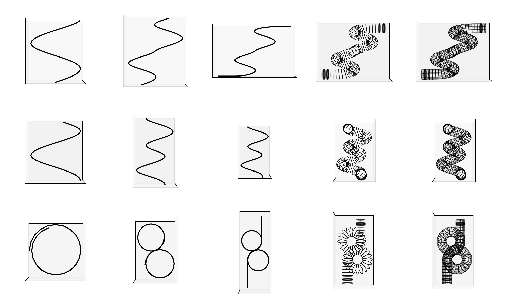
Given a set of geometric parameters, meshing was performed in Python using the classy_blocks library. Figure 5 provides some insight into how this is performed by plotting the generated mesh structure at each step of the procedure.

Figure 5: Plots in-line with the X,Y, and Z axis demonstrating the main steps within the plotting procedure for generating a coil given a set of parameters including coil radius, tube radius, pitch, inversion %, and total volume.

References

- Bergstra et al. [2011] James Bergstra, Rémi Bardenet, Yoshua Bengio, and Balázs Kégl. Algorithms for Hyper-Parameter Optimization. In J. Shawe-Taylor, R. Zemel, P. Bartlett, F. Pereira, and K.Q. Weinberger, editors, Advances in Neural Information Processing Systems, volume 24. Curran Associates, Inc., 2011. URL https://proceedings.neurips.cc/paper/2011/file/86e8f7ab32cfd12577bc2619bc635690-Paper.pdf.
- Cutajar et al. [2019] Kurt Cutajar, Mark Pullin, Andreas Damianou, Neil Lawrence, and Javier González. Deep Gaussian Processes for Multi-fidelity Modeling, 2019. URL https://arxiv.org/abs/1903.07320.
- Daniels et al. [2019] S. J. Daniels, A. A. M. Rahat, G. R. Tabor, J. E. Fieldsend, and R. M. Everson. Automated shape optimisation of a plane asymmetric diffuser using combined Computational Fluid Dynamic simulations and multi-objective Bayesian methodology. International Journal of Computational Fluid Dynamics, 33(6-7):256–271, August 2019. URL https://doi.org/10.1080/10618562.2019.1683165.
- de Brito Lira et al. [2022] Jéssica Oliveira de Brito Lira, Humberto Gracher Riella, Natan Padoin, and Cíntia Soares. Fluid dynamics and mass transfer in curved reactors: A CFD study on Dean flow effects. Journal of Environmental Chemical Engineering, 10(5):108304, October 2022. URL https://doi.org/10.1016/j.jece.2022.108304.
- Feurer and Hutter [2019] Matthias Feurer and Frank Hutter. Hyperparameter Optimization. In Automated Machine Learning, pages 3–33. Springer International Publishing, 2019. URL https://doi.org/10.1007/978-3-030-05318-5_1.
- Huang et al. [2006] D. Huang, T. T. Allen, W. I. Notz, and R. A. Miller. Sequential kriging optimization using multiple-fidelity evaluations. Structural and Multidisciplinary Optimization, 32(5):369–382, May 2006. URL https://doi.org/10.1007/s00158-005-0587-0.
- Jorayev et al. [2022] Perman Jorayev, Danilo Russo, Joshua D. Tibbetts, Artur M. Schweidtmann, Paul Deutsch, Steven D. Bull, and Alexei A. Lapkin. Multi-objective Bayesian optimisation of a two-step synthesis of p-cymene from crude sulphate turpentine. Chemical Engineering Science, 247:116938, January 2022. URL https://doi.org/10.1016/j.ces.2021.116938.
- Kandasamy et al. [2016] Kirthevasan Kandasamy, Gautam Dasarathy, Junier B. Oliva, Jeff Schneider, and Barnabas Poczos. Multi-fidelity gaussian process bandit optimisation, 2016. URL https://arxiv.org/abs/1603.06288.
- Lam et al. [2018] Rémi Lam, Matthias Poloczek, Peter Frazier, and Karen E. Willcox. Advances in Bayesian Optimization with Applications in Aerospace Engineering. In 2018 AIAA Non-Deterministic Approaches Conference. American Institute of Aeronautics and Astronautics, January 2018. URL https://doi.org/10.2514/6.2018-1656.
- Larson et al. [2019] Jeffrey Larson, Matt Menickelly, and Stefan M. Wild. Derivative-free optimization methods. Acta Numerica, 28:287–404, 2019. URL https://doi.org/10.1017/S0962492919000060.
- Lindauer et al. [2019] Marius Lindauer, Katharina Eggensperger, Matthias Feurer, André Biedenkapp, Joshua Marben, Philipp Müller, and Frank Hutter. BOAH: A Tool Suite for Multi-Fidelity Bayesian Optimization; Analysis of Hyperparameters, 2019. URL https://arxiv.org/abs/1908.06756.
- Mansour et al. [2017] M. Mansour, Z. Liu, G. Janiga, K.D.P. Nigam, K. Sundmacher, D. Thévenin, and K. Zähringer. Numerical study of liquid-liquid mixing in helical pipes. Chemical Engineering Science, 172:250–261, November 2017. URL https://doi.org/10.1016/j.ces.2017.06.015.
- Mansour et al. [2020] Michael Mansour, Prafull Khot, Dominique Thévenin, Krishna D.P. Nigam, and Katharina Zähringer. Optimal Reynolds number for liquid-liquid mixing in helical pipes. Chemical Engineering Science, 214:114522, March 2020. URL https://doi.org/10.1016/j.ces.2018.09.046.
- March et al. [2011] A. March, K. Willcox, and Q. Wang. Gradient-based multifidelity optimisation for aircraft design using Bayesian model calibration. The Aeronautical Journal (1968), 115(1174):729–738, 2011. URL https://doi.org/10.1017/S0001924000006473.
- Mateos et al. [2019] Carlos Mateos, María José Nieves-Remacha, and Juan A. Rincón. Automated platforms for reaction self-optimization in flow. Reaction Chemistry & Engineering, 4(9):1536–1544, 2019. URL https://doi.org/10.1039/c9re00116f.
- McDonough et al. [2019a] J.R. McDonough, S.M.R. Ahmed, A.N. Phan, and A.P. Harvey. The development of helical vortex pairs in oscillatory flows – A numerical and experimental study. Chemical Engineering and Processing - Process Intensification, 143:107588, September 2019a. URL https://doi.org/10.1016/j.cep.2019.107588.
- McDonough et al. [2019b] J.R. McDonough, S. Murta, R. Law, and A.P. Harvey. Oscillatory fluid motion unlocks plug flow operation in helical tube reactors at lower Reynolds numbers (Re 10). Chemical Engineering Journal, 358:643–657, February 2019b. URL https://doi.org/10.1016/j.cej.2018.10.054.
- Morita et al. [2022] Y. Morita, S. Rezaeiravesh, N. Tabatabaei, R. Vinuesa, K. Fukagata, and P. Schlatter. Applying Bayesian optimization with Gaussian process regression to computational fluid dynamics problems. Journal of Computational Physics, 449:110788, January 2022. URL https://doi.org/10.1016/j.jcp.2021.110788.
- Paleyes et al. [2019] Andrei Paleyes, Mark Pullin, Maren Mahsereci, Cliff McCollum, Neil Lawrence, and Javier González. Emulation of physical processes with emukit. In Second Workshop on Machine Learning and the Physical Sciences, NeurIPS, 2019.
- Petsagkourakis et al. [2021] Panagiotis Petsagkourakis, Benoit Chachuat, and Ehecatl Antonio del Rio-Chanona. Safe real-time optimization using multi-fidelity gaussian processes, 2021. URL https://arxiv.org/abs/2111.05589.
- Schmucker et al. [2020] Robin Schmucker, Michele Donini, Valerio Perrone, and Cedric Archambeau. Multi-objective multi-fidelity hyperparameter optimization with application to fairness. In NeurIPS 2020 Workshop on Meta-learning, 2020. URL https://www.amazon.science/publications/multi-objective-multi-fidelity-hyperparameter-optimization-with-application-to-fairness.
- Wu et al. [2019] Jian Wu, Saul Toscano-Palmerin, Peter I. Frazier, and Andrew Gordon Wilson. Practical multi-fidelity bayesian optimization for hyperparameter tuning, 2019. URL https://arxiv.org/abs/1903.04703.
- Yu and Zhu [2020] Tong Yu and Hong Zhu. Hyper-parameter optimization: A review of algorithms and applications, 2020. URL https://arxiv.org/abs/2003.05689.