Powerful Spatial Multiple Testing via Borrowing Neighboring Information

Abstract

Clustered effects are often encountered in multiple hypothesis testing of spatial signals. In this paper, we propose a new method, termed two-dimensional spatial multiple testing (2d-SMT) procedure, to control the false discovery rate (FDR) and improve the detection power by exploiting the spatial information encoded in neighboring observations. The proposed method provides a novel perspective of utilizing spatial information by gathering signal patterns and spatial dependence into an auxiliary statistic. 2d-SMT rejects the null when a primary statistic at the location of interest and the auxiliary statistic constructed based on nearby observations are greater than their corresponding thresholds. 2d-SMT can also be combined with different variants of the weighted BH procedures to improve the detection power further. A fast step-down algorithm is developed to accelerate the search for optimal thresholds in 2d-SMT. In theory, we establish the asymptotical FDR control of 2d-SMT under weak spatial dependence. Extensive numerical experiments demonstrate that the 2d-SMT method combined with various weighted BH procedures achieves the most competitive performance in FDR and power trade-off.

Keywords: Empirical Bayes; False discovery rate; Near epoch dependence; Side information.

1 Introduction

Large-scale multiple testing with spatial structure has become increasingly important in various areas, e.g., functional Magnetic Resonance Imaging (fMRI) research, genome-wide association study, environmental studies, and astronomical surveys. The essential task is identifying locations that exhibit significant deviations from the background to build scientific interpretations. Since thousands or even millions of spatially correlated hypotheses tests are often conducted simultaneously, incorporating informative spatial patterns to provide a powerful multiplicity adjustment for dependent multiple hypothesis testing is becoming a significant challenge.

There has been a growing literature on spatial signal detection with false discovery rate control (FDR, Benjamini and Hochberg, 1995). Heller et al. (2006) and Sun et al. (2015) proposed to perform multiple testing on cluster-wise hypotheses by aggregating location-wise hypotheses to increase the signal-to-noise ratio. Benjamini and Heller (2007), Sun et al. (2015) and Basu et al. (2018) defined new error rates to reflect the relative importance of hypotheses associated with different clusters. For instance, a hypothesis corresponding to a larger cluster is more important than the one associated with a smaller cluster. Scott et al. (2015) considered a two-group mixture model with the prior null probability dependent on the auxiliary spatial information. Yun et al. (2022) proposed a spatial-adaptive FDR-controlling procedure by exploiting the mirror conservativeness of the p-values under the null and the spatial smoothness under the alternative. Tansey et al. (2018) enforced spatial smoothness by imposing a penalty on the pairwise differences of log odds of hypotheses being signals between adjacent locations. Along a related line, Genovese et al. (2006) suggested to weight p-values or equivalently assign location-specific cutoffs by leveraging the tendency of hypotheses being null. This idea has been further developed in a few recent papers to incorporate different types of structural and covariate information. See, e.g., Ignatiadis et al. (2016), Li and Barber (2019), Cai et al. (2021), Zhang and Chen (2022) and Cao et al. (2022).

In many applications, signals tend to exhibit in clusters. As a result, hypotheses around a non-null location are more likely to be under the alternative than under the null. One way to account for spatially clustered signals is to screen out the locations where the average signal strength of the neighbors captured by an auxiliary statistic is weak (Shen et al., 2002). The locations passing the screening step are subjected to further analysis. This procedure suffers from the so-called selection bias as the downstream statistical inference needs to account for the selection effect from the screening step. A simple remedy is sample splitting (Wasserman and Roeder, 2009; Liu et al., 2022b), where a subsample is used to perform screening, and the remaining samples are utilized for the downstream inference. Sample splitting is intuitive and easy to implement, but it inevitably sacrifices the detection power because it does not excavate complete information. Furthermore, there are often no completely independent observations to conduct sample splitting in spatial settings.

We propose a new method named the two-dimensional spatial multiple testing (2d-SMT) procedure that fundamentally differs from the existing spatial multiple testing procedures. 2d-SMT consists of a two-dimensional rejection region built on two statistics, an auxiliary statistic $T_{1}(s)$ and a primary statistic $T_{2}(s)$, for each hypothesis. The first dimension utilizes the auxiliary information constructed from the neighbors of a location of interest to perform feature screening, which helps to increase the signal density and lessen the multiple testing burdens in the second dimension. The second dimension then uses a statistic computed from the data at the location of interest to pick out signals. 2d-SMT declares the hypothesis at location $s$ to be non-null if $T_{1}(s)\geq t_{1}$ and $T_{2}(s)\geq t_{2}$. The optimal cutoffs $t_{1}^{\star}$ and $t_{2}^{\star}$ are chosen to achieve the maximum number of discoveries while controlling the FDR at the desired level. The 2d-SMT procedure involves the following main ingredients, designed to improve its robustness and efficiency:

• Accounting for the dependence between the auxiliary statistic and the primary statistics, which alleviates the selection bias;

• Borrowing spatial signal information through an empirical Bayes approach;

• Speeding up the search for the bivariate cutoff through an efficient step-down algorithm.

2d-SMT explores spatial information from a completely different perspective than the existing weighted procedures. It thus can be combined with these methods to improve their power further. Examples of these weighted procedures include the group BH procedure (GBH, Hu et al., 2010), independent hypothesis weighting (IHW, Ignatiadis et al., 2016), structure adaptive BH algorithm (SABHA, Li and Barber, 2019), and locally adaptive weighting and screening approach (LAWS, Cai et al., 2021). The readers are referred to Section 2.7 for more details.

In a related study, Yi et al. (2021) proposed the 2dFDR approach to detect the association between omics features and covariates of interest in the presence of confounding factors. 2dFDR borrows information from confounder-unadjusted test statistics to boost the power in omics association testing with confounder-adjustment. In contrast, 2d-SMT is designed for the spatial multiple testing problem by borrowing information from neighboring observations. We develop a fast algorithm to overcome the computational bottleneck in finding the 2d cutoff values, which can be applied to both 2dFDR and 2d-SMT. Finally, it is worth mentioning that our asymptotic analysis allows weak spatial dependence, which goes beyond the independence assumption in Yi et al. (2021).

The rest of the paper is organized as follows. Section 2 develops the 2d-SMT procedure, including the oracle procedure, the feasible procedure with estimated covariance structure, and the extension by combining it with various weighted BH procedures. Section 3 discusses some implementation details and proposes an efficient algorithm to find the optimal thresholds. Section 4 establishes the asymptotic FDR control of the 2d-SMT procedure. In Section 5, extensive simulation studies demonstrate the effectiveness of the 2d-SMT procedure. Section 6 illustrates the method using an ozone dataset. Section 7 concludes and points out a few future research directions. Some additional details of the numerical experiments and technical proofs are presented in a separate online supplementary file.

2 Method

Consider a random field $\{X(s):s\in\mathcal{S}\}$ defined on a spatial domain $\mathcal{S}\subseteq\mathbb{R}^{K}$ with $K\geq 1$ that takes the form of

$$X(s)=\mu(s)+\epsilon(s),$$ (1)

where $\mu(s)$ is an unobserved process of interest and $\epsilon(s)$ is a mean-zero stationary Gaussian process. We are interested in examining whether $\mu(s)$ belongs to an indifference region $\mathcal{A}$. For example, $\mathcal{A}=\{\mu\in\mathbb{R}:\mu\leq\mu_{0}\}$ for a one-sided test and $\mathcal{A}=\{\mu\in\mathbb{R}:|\mu|\leq\mu_{0}\}$ for a two-sided test, where $\mu_{0}$ is some pre-specified value. The unobserved process $\mu(s)$, together with the indifference region $\mathcal{A}$, induces a background statement $\theta(s)=\bm{1}\{\mu(s)\not\in\mathcal{A}\}$ on the spatial domain $\mathcal{S}$. We define $\mathcal{S}_{0}=\{s\in\mathcal{S}:\theta(s)=0\}$ and $\mathcal{S}_{1}=\{s\in\mathcal{S}:\theta(s)=1\}$ as the sets of null and non-null locations respectively. We focus on the point-wise analysis, where we are interested in testing the hypothesis

$$\mathcal{H}_{0,s}:\mu(s)\in\mathcal{A}\quad\text{versus}\quad\mathcal{H}_{a,s}:\mu(s)\notin\mathcal{A}.$$

At each location $s\in\mathcal{S}$, we make a decision $\delta(s)$, where $\delta(s)=1$ if $\mathcal{H}_{0,s}$ is rejected and $\delta(s)=0$ otherwise. Let $\Delta_{1}=\{s\in\mathcal{S}:\delta(s)=1\}$ be the set of rejections associated with the decision rule $\delta$. The false discovery rate (FDR) is defined as

$$\text{FDR}=\mathbb{E}\left(\frac{|\Delta_{1}\cap\mathcal{S}_{0}|}{1\vee|\Delta_{1}|}\right),$$

where $|\cdot|$ denotes the cardinality of a generic set and $\Delta_{1}\cap\mathcal{S}_{0}$ is the set of false rejections.

We next present a novel spatial multiple testing procedure that borrows neighboring information to improve the power of signal detection without sacrificing the FDR control.

2.1 Motivation

For clarity, we focus our discussions on the one-sided test in the rest of this paper, i.e.,

$$\mathcal{H}_{0,s}:\mu(s)\leq 0\quad\text{versus}\quad\mathcal{H}_{a,s}:\mu(s)>0.$$

For each location $s\in\mathcal{S}$, we define a set of its neighborhood as $\mathcal{N}(s)\subseteq\mathcal{S}\backslash\{s\}$. Because of the spatial dependence and smoothness encountered in many real applications, the set of neighboring observations $\{X(v):v\in\mathcal{N}(s)\}$ is expected to provide useful side information on determining the state of $\theta(s)$. To formalize this idea, we consider two statistics, namely the auxiliary statistic

$$T_{1}(s)=\frac{1}{\tau(s)}\sum_{v\in\mathcal{N}(s)}X(v)$$ (2)

based on the averaged observed values in the neighborhood of $s$ and the primary statistic $T_{2}(s)=\sigma^{-1}(s)X(s)$ based on the observation from the location of interest, where $\sigma^{2}(s)=\mathrm{var}\{\epsilon(s)\}$ and $\tau^{2}(s)=\sum_{v,v^{\prime}\in\mathcal{N}(s)}\mathrm{cov}\left\{\epsilon(v),\epsilon(v^{\prime})\right\}$. Under the null $\mathcal{H}_{0}(s)$, we have

$$\left(\begin{array}[]{c}T_{1}(s)\\ T_{2}(s)\end{array}\right)=\left(\begin{array}[]{c}\xi(s)\\ \sigma^{-1}(s)\mu(s)\end{array}\right)+\left(\begin{array}[]{c}V_{1}(s)\\ V_{2}(s)\end{array}\right),$$

where $\xi(s)=\tau^{-1}(s)\sum_{v\in\mathcal{N}(s)}\mu(v)$ and

$$\left(\begin{array}[]{c}V_{1}(s)\\ V_{2}(s)\end{array}\right)\sim\mathcal{N}\left(\left(\begin{array}[]{c}0\\ 0\end{array}\right),\left(\begin{array}[]{cc}1&\rho(s)\\ \rho(s)&1\end{array}\right)\right)$$

with $\rho(s)=\{\sigma(s)\tau(s)\}^{-1}\sum_{v\in\mathcal{N}(s)}\mathrm{cov}\{\epsilon(s),\epsilon(v)\}$. Our method is motivated by the following two-stage procedure. Specifically, at stage 1, we use the auxiliary statistic $T_{1}(s)$ to screen out the nulls based on the belief that observations around a non-null location are likely to take larger values on average. At stage 2, we use $T_{2}(s)$ to pick out signals among those who survive from stage 1. Given the thresholds $(t_{1},t_{2})$ for the two stages, the procedure can be described as follows:

• Use the auxiliary statistic $T_{1}(s)$ to determine a preliminary set of signals $\mathcal{D}_{1}=\left\{s\in\mathcal{S}:T_{1}(s)\geq t_{1}\right\}$.

• Reject $\mathcal{H}_{0,s}$ for $T_{2}(s)\geq t_{2}$ and $s\in\mathcal{D}_{1}$. As a result, the final set of discoveries is given by $\mathcal{D}_{2}=\left\{s\in\mathcal{S}:T_{1}(s)\geq t_{1},T_{2}(s)\geq t_{2}\right\}$.

Due to the screening step that reduces the multiple testing burden for the second stage, we expect the above procedure to be more powerful than the traditional procedure based only on the primary statistic. Indeed, the traditional 1d rejection region is a special case of the 2d rejection region $\left\{s\in\mathcal{S}:T_{1}(s)\geq t_{1},T_{2}(s)\geq t_{2}\right\}$ by setting $t_{1}\leq\min_{s\in\mathcal{S}}T_{1}(s)$, i.e., the screening stage preserves all locations. If we select the two thresholds one by one, then the choice of $t_{2}$ needs to account for the selection effect from the first stage. Here we propose a new method to address this issue by simultaneously selecting the two thresholds, which we name it the 2-dimensional (2d) procedure.

2.2 Approximation of the false discovery proportion

Note that $\mathcal{H}_{0,s}$ is rejected when $T_{1}(s)\geq t_{1}$ and $T_{2}(s)\geq t_{2}$. Recalling that $\mathcal{S}_{0}$ is the set of true nulls, FDP is then given by

$$\operatorname{FDP}(t_{1},t_{2})=\frac{\sum_{s\in\mathcal{S}_{0}}\mathbf{1}\left\{T_{1}(s)\geq t_{1},T_{2}(s)\geq t_{2}\right\}}{1\vee R(t_{1},t_{2})},$$

where $R(t_{1},t_{2})=\sum_{s\in\mathcal{S}}\mathbf{1}\left\{T_{1}(s)\geq t_{1},T_{2}(s)\geq t_{2}\right\}$ corresponds to the total number of rejections. As $\mu(s)\leq 0$ for $s\in\mathcal{S}_{0}$, we have

$$\operatorname{FDP}(t_{1},t_{2})\leq \frac{\sum_{s\in\mathcal{S}_{0}}\mathbf{1}\left\{V_{1}(s)+\xi(s)\geq t_{1},V_{2}(s)\geq t_{2}\right\}}{1\vee R(t_{1},t_{2})}.$$

Replacing the number of false rejections in the numerator of the RHS above by its expected value, we obtain the approximated upper bound on the FDP as

$$\operatorname{FDP}(t_{1},t_{2})\lesssim\frac{\sum_{s\in\mathcal{S}_{0}}\mathbb{P}\left\{V_{1}(s)+\xi(s)\geq t_{1},V_{2}(s)\geq t_{2}\right\}}{1\vee R(t_{1},t_{2})}.$$ (3)

The major challenge here is the estimation of the expected number of false rejections given by $\sum_{s\in\mathcal{S}_{0}}\mathbb{P}\left\{V_{1}(s)+\xi(s)\geq t_{1},V_{2}(s)\geq t_{2}\right\}$, which involves a large number of nuisance parameters $\xi(s)$’s. To overcome the difficulty, we shall adopt a Bayesian viewpoint by assuming that $\{\xi(s):s\in\mathcal{S}\}$ follow a common prior distribution. The Bayesian viewpoint allows us to borrow spatial information across different locations to directly estimate the expected number of false rejections without estimating individual $\xi(s)$ at each location explicitly.

2.3 Nonparametric empirical Bayes

Suppose $\xi(s)$ are independently generated from a common prior distribution $G_{0}$. We aim to estimate $G_{0}$ based on the set of auxiliary statistics $\{T_{1}(s):s\in\mathcal{S}\}$ through the nonparametric empirical Bayes (NPEB) approach. It can be achieved by maximizing the marginal distribution of $T_{1}(s)=\xi(s)+V_{1}(s)$, which is given by $f_{G_{0}}(x)=\int\phi(x-u)dG_{0}(u)$ with $\phi$ denoting the density function of standard normal distribution.

Classical empirical Bayes methods often assume independence among the observations, which is violated in our case due to the spatial dependence. To reduce the dependence, we select a subset $\widetilde{\mathcal{S}}$ of $\mathcal{S}$ such that any two points in $\widetilde{\mathcal{S}}$ have a distance larger than some threshold $c_{0}$ (so that the dependence between $T_{1}(v)$ and $T_{1}(v^{\prime})$ for any $v,v^{\prime}\in\widetilde{\mathcal{S}}$ is sufficiently weak). Following Kiefer and Wolfowitz (1956) and Jiang and Zhang (2009), we consider the general maximum likelihood estimator (GMLE) defined as

$$\widetilde{G}_{\widetilde{\mathcal{S}}}=\mathop{\mbox{arg\,max}}_{G\in\mathcal{G}}\sum_{s\in\widetilde{\mathcal{S}}}\log f_{G}\{T_{1}(s)\},$$ (4)

where $\mathcal{G}$ represents the set of all probability distributions on $\mathbb{R}$ and $f_{G}(x)=\int\phi(x-u)dG(u)$ is the convolution between $G$ and $\phi$. The optimization in (4) can be cast as a convex optimization problem that can be efficiently solved by modern interior point methods. The readers are referred to Koenker and Mizera (2014) and Koenker and Gu (2017) for more detailed discussions.

2.4 2d spatial multiple testing procedure

We now describe a procedure to select two thresholds simultaneously. Define

$$L\left\{t_{1},t_{2},\xi(s),\rho(s)\right\}=\mathbb{P}\left\{V_{1}(s)+\xi(s)\geq t_{1},V_{2}(s)\geq t_{2}\mid\xi(s)\right\}.$$

Given the GMLE $\widetilde{G}_{\widetilde{\mathcal{S}}}$ in (4) as the prior distribution and in view of (3), we consider an approximated upper bound for $\mathrm{FDP}(t_{1},t_{2})$ as

$$\widetilde{\text{FDP}}(t_{1},t_{2}):=\frac{\sum_{s\in\mathcal{S}}\int L\left\{t_{1},t_{2},x,\rho(s)\right\}d\widetilde{G}_{\widetilde{\mathcal{S}}}(x)}{1\vee R(t_{1},t_{2})}.$$

For a desired FDR level $q\in(0,1)$, the proposed 2d-SMT procedure chooses the optimal threshold such that

$$(\widehat{t}^{\star}_{1},\widehat{t}^{\star}_{2})=\mathop{\mbox{arg\,max}}_{(t_{1},t_{2})\in\mathcal{F}_{q}}R(t_{1},t_{2}),$$ (5)

where $\mathcal{F}_{q}=\{(t_{1},t_{2})\in\mathbb{R}^{2}:\widetilde{\text{FDP}}(t_{1},t_{2})\leq q\}$.

We argue that 2d-SMT is, in general, more powerful than the classical BH procedure based on the primary statistics alone. The intuition is that for a small enough $t_{1}$, the first dimension does not screen out any null hypothesis and only the second dimension is effective in identifying signals. In this case, we note that

$$\int L\left\{t_{1},t_{2},x,\rho(s)\right\}d\widetilde{G}_{\widetilde{\mathcal{S}}}(x) \approx\mathbb{P}\{V_{2}(s)\geq t_{2}\}\quad\mbox{and}\quad R(t_{1},t_{2})=\sum_{s\in\mathcal{S}}\mathbf{1}\left\{T_{2}(s)\geq t_{2}\right\},$$

which implies that

$$\widetilde{\text{FDP}}(t_{1},t_{2})\approx\frac{\sum_{s\in\mathcal{S}}\mathbb{P}\{V_{2}(s)\geq t_{2}\}}{1\vee\sum_{s\in\mathcal{S}}\mathbf{1}\left\{T_{2}(s)\geq t_{2}\right\}}.$$ (6)

Finding the optimal cutoff $t_{2}^{\#}$ that maximizes the number of rejections while controls the RHS of (6) at level $q$ is equivalent to applying the BH procedure to the primary statistics. Since the 2d-SMT procedure has the flexibility to choose an additional cutoff $t_{1}$ to maximize the number of rejections, it guarantees to make more rejections. As we will show in Section 4, 2d-SMT procedure provides asymptotic FDR control, and thus the higher number of rejections typically translates into a higher power.

Remark 1.

Shen et al. (2002) and Huang et al. (2021) considered the case where $\mu$ has a sparse wavelet representation. The goal is to test the global null $\mu(s)=0$ for all $s$ and detect the significant wavelet coefficients while controlling the FDR. Observing that the wavelet coefficients within each scale and across different scales are related, they screened the wavelet coefficients based on the largest adjacent wavelet coefficients to gain more power. The generalized degrees of freedom determine the number of locations for the subsequent FDR-controlling procedure. Our approach can be potentially applied to their settings by exploring the signal structure encoded in the neighboring wavelet coefficients.

2.5 Estimating the null proportion

It is well known that when the number of signals is a substantial proportion of the total number of hypotheses, the BH procedure will be overly conservative. We develop a new estimator of the proportion of true null hypotheses in our setting, which is a modification of Storey’s approach (Storey, 2002; Storey et al., 2004). As a motivation, we assume that $T_{2}(s)$ approximately follows the mixture model

$$T_{2}(s)\sim\pi_{0}\mathcal{N}(\mu_{0}(s),1)+(1-\pi_{0})\mathcal{N}(\mu_{1}(s),1),$$

where $\mu_{0}(s)\leq 0$, $\mu_{1}(s)>0$, and $\pi_{0}$ denotes the prior probability that $s\in\mathcal{S}_{0}$. Let $\Phi$ be the cumulative distribution function (CDF) of the standard normal distribution. Fixing some $\lambda\in\mathbb{R}$, we have

$$\mathbb{P}\{T_{2}(s)<\lambda\} =\pi_{0}\mathbb{P}\{\mathcal{N}(\mu_{0}(s),1)<\lambda\}+(1-\pi_{0})\mathbb{P}\{\mathcal{N}(\mu_{1}(s),1)<\lambda\}$$

$$\geq\pi_{0}\mathbb{P}\{\mathcal{N}(\mu_{0}(s),1)<\lambda\}$$

$$\geq\pi_{0}\Phi(\lambda),$$

where the second line is tighter if $(1-\pi_{0})\mathbb{P}\{\mathcal{N}(\mu_{1}(s),1)<\lambda\}$ is closer to zero and the third line becomes equality when $\mu_{0}(s)=0$. The above derivation suggests a conservative estimator for $\pi_{0}$ given by

$$\widehat{\pi}_{0}:=\frac{\sum_{s\in\mathcal{S}}\bm{1}\{T_{2}(s)<\lambda\}}{\left|\mathcal{S}\right|\Phi(\lambda)}\approx\frac{\mathbb{P}\{T_{2}(s)<\lambda\}}{\Phi(\lambda)}\geq\pi_{0}.$$ (7)

2.6 A feasible procedure

So far we have assumed that the spatial covariance function $k(s,s^{\prime})=\text{cov}\{\epsilon(s),\epsilon(s^{\prime})\}$ of the error process is known. In practice, we need to estimate the spatial covariance function $\text{cov}\{\epsilon(s),\epsilon(s^{\prime})\}$, which has been widely investigated in the literature (Sang and Huang, 2012; Padoan and Bevilacqua, 2015; Sommerfeld et al., 2018; Katzfuss and Guinness, 2021); see Section LABEL:sec:cov_est of the Supplementary Materials for more details. Given the estimated covariance function, we let $\widehat{T}_{1}(s)$ and $\widehat{T}_{2}(s)$ respectively denote the feasible statistics of $T_{1}(s)$ and $T_{2}(s)$ by replacing $(\sigma(s),\tau(s),\rho(s))$ with their estimates $(\widehat{\sigma}(s),\widehat{\tau}(s),\widehat{\rho}(s))$. Define the nonparametric empirical Bayes estimate of $G_{0}$ based on $\{\widehat{T}_{1}(s):s\in\widetilde{\mathcal{S}}\}$ as $\widehat{G}_{\widetilde{\mathcal{S}}}(u)$. We propose the following FDP estimate which accounts for the null proportion using the idea in Section 2.5,

$$\widehat{\operatorname{FDP}}_{\lambda,\widetilde{\mathcal{S}}}(t_{1},t_{2}):=\frac{\sum_{s\in\mathcal{S}}\bm{1}\{\widehat{T}_{2}(s)<\lambda\}}{m\Phi(\lambda)}\frac{\sum_{s\in\mathcal{S}}\int L\left\{t_{1},t_{2},x,\widehat{\rho}(s)\right\}d\widehat{G}_{\widetilde{\mathcal{S}}}(x)}{1\vee\widehat{R}(t_{1},t_{2})},$$ (8)

where $\widehat{R}(t_{1},t_{2})=\sum_{s\in\mathcal{S}}\mathbf{1}\big{\{}\widehat{T}_{1}(s)\geq t_{1},\widehat{T}_{2}(s)\geq t_{2}\big{\}}$. Thus, given the desired FDR level $q\in(0,1)$, the optimal rejection thresholds are defined as

$$(\widetilde{t}_{1}^{\star},\widetilde{t}_{2}^{\star})=\mathop{\mbox{arg\,max}}_{(t_{1},t_{2})\in\mathcal{F}_{q}}\widehat{R}(t_{1},t_{2}),$$ (9)

where $\mathcal{F}_{q}=\{(t_{1},t_{2})\in\mathbb{R}^{2}:\widehat{\operatorname{FDP}}_{\lambda,\widetilde{\mathcal{S}}}(t_{1},t_{2})\leq q\}$. The left panel in Figure 1 exemplifies the thresholds for the BH and 2d-SMT procedures with the nominal FDR level at 10%. Compared to the BH procedure, the 2d-SMT procedure realizes a lower threshold for $T_{2}(s)$ (the red vertical line) because it excludes locations exhibiting weak neighboring signals with a threshold for $T_{1}(s)$ (the red horizontal line). The lower threshold for $T_{2}(s)$ in 2d-SMT leads to more true rejections in this example.

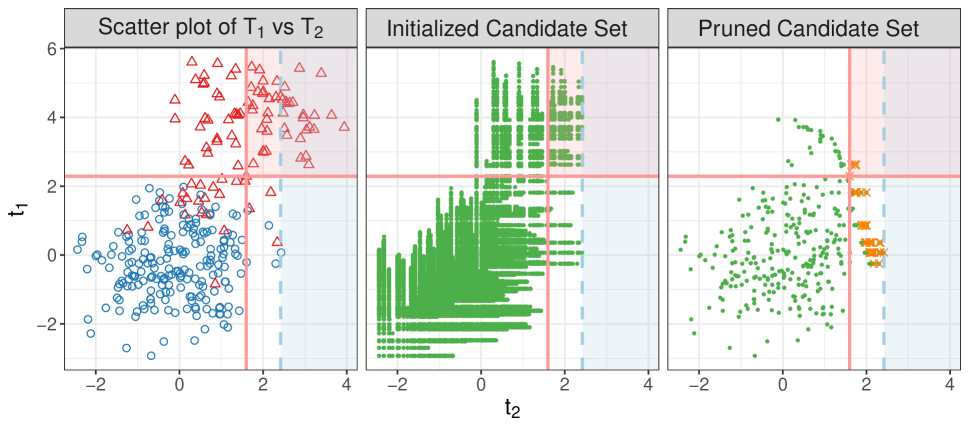
Figure 1: An illustration of the proposed 2d-SMT procedure and fast step-down algorithm. The spatial domain $\mathcal{S}$ includes 300 points. The red triangle ($\triangle$) and blue circle ($\circ$) in the left panel denote non-null and null locations, respectively. The solid and dashed lines are the thresholds for 2d-SMT procedure and BH procedure, respectively. The orange cross ($\times$) in the right panel corresponds to the cutoff whose corresponding FDP is less than 0.1. The set $\mathcal{T}^{\prime}$ in the middle panel contains 14,534 points, whereas the set after our proposed pruning steps in the right panel significantly reduces the number of candidates to 345.

2.7 Spatial varying null proportions and cutoffs

Our proposed 2d-SMT is a flexible framework that can accommodate weighted BH procedures (wBH), a broad class of multiple testing procedures. wBH leverages the hypothesis heterogeneity by assigning location-specific cutoffs. According to wBH, $\mathcal{H}_{0,s}$ will be rejected with the rule $p(s):=1-\Phi(\widehat{T}_{2}(s))\leq\min\{\tau,w(s)t\}$, $\tau\in(0,1]$, where $\tau$ is the censoring level for all p-values and $w(s)$ is a location-specific weight that encodes external information for location $s$. Apparently, the rejection rule is equivalent to assigning location-specific cutoffs to the primary statistics, i.e., $\widehat{T}_{2}(s)\geq\Phi^{-1}(1-\min\{\tau,w(s)t\})$. Inspired by the idea behind wBH, we extend 2d-SMT by allowing location-specific cutoffs to further incorporate external information on the prior null probability and signal distribution. Specifically, we reject $\mathcal{H}_{0,s}$ whenever $\widehat{T}_{1}(s)\geq c(t_{1},s)$ and $\widehat{T}_{2}(s)\geq c(t_{2},s)$, where $c(t,s)=\Phi^{-1}(1-\min\{\tau,w(s)t\})$. With some abuse of notation, we let

$$\widehat{\operatorname{FDP}}_{\lambda,\widetilde{\mathcal{S}}}(t_{1},t_{2}):=\frac{\sum_{s\in\mathcal{S}}\widehat{\pi}_{0}(s)\int L\left\{c(t_{1},s),c(t_{2},s),x,\widehat{\rho}(s)\right\}d\widehat{G}_{\widetilde{\mathcal{S}}}(x)}{1\vee\widehat{R}(t_{1},t_{2})},$$ (10)

where $\widehat{\pi}_{0}(s)$ is an estimate of the null proportion $\pi_{0}(s)=\mathbb{P}\{\theta(s)=0\}$ at location $s$. We reject $\mathcal{H}_{0,s}$ if $T_{1}(s)\geq c(\widetilde{t}_{1}^{\star},s)$ and $T_{2}(s)\geq c(\widetilde{t}_{2}^{\star},s)$, where $(\widetilde{t}_{1}^{\star},\widetilde{t}_{2}^{\star})$ is the solution to (9) with the FDP estimate given in (10).

There have been extensive recent studies on the choice of $w(s)$ in wBH. Examples include GBH (Hu et al., 2010), IHW (Ignatiadis et al., 2016; Ignatiadis and Huber, 2021), SABHA (Li and Barber, 2019) and LAWS (Cai et al., 2021). The weights in these examples are either proportional to $1/\pi_{0}(s)$ or $\{1-\pi_{0}(s)\}/\pi_{0}(s)$, where $\pi_{0}(s)$ can be estimated using various approaches. In the spatial setting, we often use the location associated with each hypothesis as the external covariate to estimate $\pi_{0}(s)$.

3 Implementation Details

In this section, we discuss a few crucial points for the implementation of our method. First of all, the auxiliary statistic $\widehat{T}_{1}(s)$ requires the specification of a pre-chosen neighborhood $\mathcal{N}(s)$ for each location. In our implementation, we let $\mathcal{N}(s)$ be the set of the $\kappa$-nearest neighbors around location $s$, and find that 2d-SMT is not quite sensitive to the choice of $\kappa$ and deliver satisfactory power improvement provided $2\leq\kappa\leq 7$; see Section LABEL:sec:rob_nei_num of the Supplementary Materials for more details. Generally, the neighborhood $\mathcal{N}(s)$ can be determined using external/side information that is independent of the data $\{X(s):s\in\mathcal{S}\}$.

Second, the auxiliary statistics used in NPEB estimation, $\{\widehat{T}_{1}(s):s\in\widetilde{\mathcal{S}}\}$, should be from far enough spatial locations to weaken their spatial dependency. In practice, we choose $\widetilde{\mathcal{S}}\subset\mathcal{S}$ whose neighbors have no overlaps.

Third, when the signal is sparse, the estimation of the number of false rejections in 2d-SMT procedure may be unstable. Inspired by the idea of Knockoff+, we add a small offset to improve the selection stability. More precisely, we replace $\sum_{s\in\mathcal{S}}\int L\left\{t_{1},t_{2},x,\widehat{\rho}(s)\right\}d\widehat{G}_{\widetilde{\mathcal{S}}}(x)$ in (8) by $\sum_{s\in\mathcal{S}}\int L\left\{t_{1},t_{2},x,\widehat{\rho}(s)\right\}d\widehat{G}_{\widetilde{\mathcal{S}}}(x)+q$, where $q$ is the target FDR level. This replacement improves the selection stability for sparse signals but does not influence the performance of power and FDR control for dense signals.

Finally, finding the optimal thresholds in 2d-SMT requires solving the discrete constrained optimization problem (9). Due to the discrete nature of (9), the solution can be obtained if we replace $\mathcal{F}_{q}$ by

$$\{(t_{1},t_{2})\in\mathcal{T}:\widehat{\operatorname{FDP}}_{\lambda,\widetilde{\mathcal{S}}}(t_{1},t_{2})\leq q\},$$

where $\mathcal{T}=\{(\widehat{T}_{1}(s),\widehat{T}_{2}(s^{\prime})):s,s^{\prime}\in\mathcal{S}\}$ is the set of all candidate cutoff values. A naive grid search algorithm would require evaluating $\widehat{\operatorname{FDP}}_{\lambda,\widetilde{\mathcal{S}}}$ at $|\mathcal{S}|^{2}$ different values, which is computationally prohibitive for a large number of spatial locations. To overcome the computational bottleneck, we propose a fast step-down algorithm to utilize the specific structure of (9) through the following three steps. We briefly introduce the basic idea below and defer the comprehensive discussion to Section LABEL:ref:searching_alg of the Supplementary Materials.

Step 1. We maintain the cutoffs that achieve the minimum FDP among all the cutoffs realizing the same rejection sets. The derivation in Section LABEL:ref:searching_alg of the Supplementary Materials suggests that we only need to consider the following set of candidate cutoff values:

$$\mathcal{T}^{\prime}=\left\{(\widehat{T}_{1}(s_{l}),\widehat{T}_{2}(s_{k})):\widehat{T}_{1}(s_{l})\leq\widehat{T}_{1}(s_{k})\mbox{ and }l\leq k,\,k=1,2,\ldots,m\right\}\cup\left\{(\infty,\infty)\right\}.$$

Step 2. Let $\widetilde{t}_{2}^{\#}$ be the minimum value satisfying $\widehat{\operatorname{FDP}}_{\lambda,\widetilde{\mathcal{S}}}(-\infty,t_{2})\leq q$. It is not hard to see that the optimal cutoff for the primary statistic in 2d-SMT is no more than $\widetilde{t}_{2}^{\#}$. Hence we can reduce the set of candidate cutoffs to $\mathcal{T}^{\prime\prime}=\left\{(t_{1},t_{2})\in\mathcal{T}^{\prime}:t_{2}\leq\widetilde{t}_{2}^{\#}\right\}$.
Step 3. Denote the elements in $\mathcal{T}^{\prime\prime}$ by $(t_{1,i,j},t_{2,i})$ for $i=1,2\dots,\breve{m}$ and $j=1,\dots,m_{i}$, where $\breve{m}$ is the number of $\widehat{T}_{2}(s)$’s that are smaller than or equal to $\widetilde{t}_{2}^{\#}$. Suppose the points are sorted in the following way: (1) $t_{2,1}>t_{2,2}>\cdots>t_{2,\breve{m}}$; (2) $t_{1,i,1}>t_{1,i,2}>\cdots>t_{1,i,m_{i}}$ for all $1\leq i\leq\breve{m}$. Our algorithm involves two loops. In the outer loop, we search the cutoff for the primary statistic, while in the inner loop, we search the cutoff for the auxiliary statistic. The key idea here is to skip those cutoffs in the inner loop that are impossible to procedure a value of $\widehat{\operatorname{FDP}}$ equal to or below the level $q$. For example, consider a cutoff $(t_{1,i,j},t_{2,i})$ which induces $R$ rejections with $\widehat{\operatorname{FDP}}_{\lambda,\widetilde{\mathcal{S}}}(t_{1,i,j},t_{2,i})=2q$. Then the next cutoff, denoted as $(t_{1,i,j^{\prime}},t_{2,i})$, needs to induce at least $2R$ rejections to ensure that $\widehat{\operatorname{FDP}}_{\lambda,\widetilde{\mathcal{S}}}(t_{1,i,j^{\prime}},t_{2,i})\leq q$. When there is no tie, increasing $j$ by $k$ brings exactly $k$ more rejections. Therefore, the next possible cutoff to be examined is $(t_{1,i,j+R},t_{2,i})$. The middle and left panels in Figure 1 illustrate how the set of candidate cutoff values can be reduced by Step 3.

Algorithm 1 Fast Step-down Algorithm.

Input: Test Statistics $\left\{\left(\widehat{T}_{1}(s),\widehat{T}_{2}(s)\right):s\in\mathcal{S}\right\}$; target FDR level $q$;

Initialization:

1:Initialize $(\widetilde{t}_{1}^{\star},\widetilde{t}_{2}^{\star},R_{\max},\operatorname{FDP}_{\min})=\left(-\infty,\widetilde{t}_{2}^{\#},\widehat{R}(-\infty,\widetilde{t}_{2}^{\#}),\widehat{\operatorname{FDP}}_{\lambda,\widetilde{\mathcal{S}}}(-\infty,\widetilde{t}_{2}^{\#})\right)$

Search Step:

1:for $i=1,2,\ldots,\breve{m}$ do

2:    Calculate $R=\widehat{R}(t_{1,i,1},t_{2,i})$;

3:    Set $j=1+\max(0,R_{\max}-R)$;

4:    while $j\leq m_{i}$ do

5:         Calculate $R=\widehat{R}(t_{1,i,j},t_{2,i})$ and $\widehat{\operatorname{FDP}}=\widehat{\operatorname{FDP}}_{\lambda,\widetilde{\mathcal{S}}}(t_{1,i,j},t_{2,i})$ according to (8);

6:         if $R=R_{\max}$ and $\widehat{\operatorname{FDP}}<\operatorname{FDP}_{\min}$ or $R>R_{\max}$ and $\widehat{\operatorname{FDP}}\leq q$ then

7:             $(\widetilde{t}_{1}^{\star},\widetilde{t}_{2}^{\star},R_{\max},\operatorname{FDP}_{\min})=(t_{1,i,j},t_{2,i},R,\widehat{\operatorname{FDP}})$;

8:             Update $j=j+1$;

9:         else

10:             Calculate $R_{\text{req}}=\lceil\widehat{\operatorname{FDP}}\times R/q\rceil$;

11:             Update $j=j+\max(1,R_{\text{req}}-R)$;

12:         end if

13:    end while

14:end for

Output: Rejection threshold $(\widetilde{t}_{1}^{\star},\widetilde{t}_{2}^{\star})$.

4 Asymptotic results

In this section, we investigate the asymptotic property of the proposed 2d-SMT procedure. We observe $\{X(s):s\in\mathcal{S}_{m}\}$, where $\mathcal{S}_{m}=\{s_{1},s_{2},\cdots,s_{m}\}\subseteq\mathcal{S}\subseteq\mathbb{R}^{K}$. We denote by $\mathcal{S}_{0,m}=\mathcal{S}_{m}\cap\mathcal{S}_{0}$ with $m_{0}=|\mathcal{S}_{0,m}|$ the set of null locations and let $\mathcal{S}_{1,m}=\mathcal{S}_{m}\cap\mathcal{S}_{1}$ with $m_{1}=|\mathcal{S}_{1,m}|$ be the set of non-null locations. We further let $\widetilde{\mathcal{S}}_{m}\subseteq\mathcal{S}_{m}$ with $|\widetilde{\mathcal{S}}_{m}|=\tilde{m}$ be the set of locations for implementing the NPEB. Our asymptotic analysis requires the following regularity conditions.

Assumption 1 (Spatial Domain).

The spatial domain $\mathcal{S}\subset\mathbb{R}^{K}$ is infinitely countable. Further, there exist $0<\Delta_{l}<\Delta_{u}<\infty$, such that for every element in $\mathcal{S}$, the distance to its nearest neighbor is bounded from below and above respectively by $\Delta_{l}$ and $\Delta_{u}$, i.e.,

$$\Delta_{l}\leq\inf_{\begin{subarray}{c}s^{\prime}\in\mathcal{S}\\ s^{\prime}\neq s\end{subarray}}\mathrm{dist}(s,s^{\prime})\leq\Delta_{u},~{}\forall s\in\mathcal{S},$$

where $\mathrm{dist}(\cdot,\cdot)$ denotes the Euclidean distance of two points.

Assumption 1 states that the distance between any location in $\mathcal{S}$ and its nearest neighbor is moderately uniform. One example satisfying Assumption 1 is the lattice $\mathcal{S}=\mathbb{Z}^{K}$ where $\Delta_{l}=\Delta_{u}=1$. Particularly, the lower bound ensures $\max_{s,s^{\prime}\in\mathcal{S}_{m}}\mathrm{dist}(s,s^{\prime})$ tends to infinity as $m$ increases.

Assumption 2 (Neighborhood).

For each location $s$ in $\mathcal{S}$, its neighborhood $\mathcal{N}(s)\subset\mathcal{S}\backslash\{s\}$ used in 2d-SMT is its nearest neighbors with size uniformly upper bounded by some positive integer $N_{nei}\in\mathbb{N}^{+}$, i.e., $0<|\mathcal{N}(s)|<N_{nei},~{}\forall s\in\mathcal{S}.$

Assumption 2 specifies the neighborhood set of each location and requires the number of locations in each neighborhood to be bounded.

Assumption 3 (Second-order Structure).

The variance and covariance of the error process $\epsilon(s)$ satisfy

(a)  There exist positive constants $B_{ud,\sigma}$, $B_{up,\sigma}$, $B_{ud,\tau}$, and $B_{up,\tau}$, such that $B_{ud,\sigma}\leq\inf_{s\in\mathcal{S}}\sigma(s)\leq\sup_{s\in\mathcal{S}}\sigma(s)<B_{up,\sigma}$ and $B_{ud,\tau}\leq\inf_{s\in\mathcal{S}}\tau(s)\leq\sup_{s\in\mathcal{S}}\tau(s)<B_{up,\tau}$ for all $s\in\mathcal{S}$;
(b)  The estimated covariance of $X$ are uniformly weakly consistent with a polynomial rate, i.e., $\sup_{s,s^{\prime}\in\mathcal{S}_{m}}|\widehat{\mathrm{cov}}\{\epsilon(s),\epsilon(s^{\prime})\}-\mathrm{cov}\{\epsilon(s),\epsilon(s^{\prime})\}|=o_{\mathbb{P}}(m^{-q})$ for some $q>0$.

Assumptions 3 requires the variance of the error process to be bounded away from zero and infinity. Assumption 3 imposes requirement on the convergence rate of the covariance function estimate, which is satisfied by many commonly-used estimators. For example, the maximum likelihood estimator achieves the desired rate of convergence with $q=1/2$ when the parametric covariance function is locally Lipschitz continuous (Mardia and Marshall, 1984).

To describe the spatial dependence structure, we adopt the near epoch dependency (NED) that was first introduced to the spatial analysis in Jenish and Prucha (2012) and has become popular since then. Denote by $\mathcal{V}$ a spatial domain such that $\mathcal{S}\subseteq\mathcal{V}\subset\mathbb{R}^{K}$ for $K\geq 1$. Let $\left\{Y(v),v\in\mathcal{V}\right\}$ be a random field and set $\mathfrak{F}(S)=\sigma\left\{Y(s),s\in S\right\}$ as the $\sigma$-field generated by $Y(s)$ for $s\in S\subset\mathcal{V}$.

Definition 1 (Near Epoch Dependency).

Let $X=\{X(s),s\in\mathcal{S}_{m}\}$ be a random field with $\|X(s)\|_{p}<\infty$ where $\|X(s)\|_{p}=(\mathbb{E}|X(s)|^{p})^{1/p}$, $p\geq 1$. Define $Y=\{Y(s),s\in\mathcal{V}_{m}\}$ as a random field where $\mathcal{S}_{m}\subseteq\mathcal{V}_{m}$ and let $\mathbf{d}=\{d_{m}(s),s\in\mathcal{S}_{m}\}$ be a set of finite positive constants. Then, the random field $X$ is said to be $L_{p}(\mathbf{d})$-near-epoch dependent on the random field $Y$ if

$$\left\|X(s)-\mathbb{E}\left\{X(s)\mid\mathfrak{F}(S)\right\}\right\|_{p}\leq d_{m}(s)\psi(r),$$

where $S\subset\mathcal{V}_{m}$, $r=\max\left\{t\geq 0:B(s;t)\subseteq S\right\}$ with $B(s;t)$ being a ball centered around $s$ with radius $t$, and $\psi(r)\geq 0$ is some non-increasing sequence with $\lim_{r\rightarrow\infty}\psi(r)=0$. Here $\psi(r)$ and $d_{m}(s)$ are called NED coefficients and NED scaling factors, respectively. We say $X$ is $L_{p}(\mathbf{d})$-NED of size $-\lambda$ if $\psi(r)=O(r^{-\mu})$ for some $\mu>\lambda>0$. Furthermore, if $\sup_{m}\sup_{s\in\mathcal{S}_{m}}d_{m}(s)<\infty$, then $X$ is said to be uniformly $L_{p}$-NED on $Y$.

Assumption 4 (Uniform Near Epoch Dependency).

$X=\{X(s),s\in\mathcal{S}_{m}\}$ is uniformly $L_{p}$-NED on $Y=\{Y(s):s\in\mathcal{V}_{m}\}$ of size $-\lambda$, for $\lambda>0$, $p\geq 2$, where $Y(s)$ are independently distributed.

In Definition 1, $B(s;t)$ is the maximum ball that is completely included in $S$. The quantity $\|X(s)-\mathbb{E}\{X(s)\mid\mathfrak{F}(S)\}\|_{p}$ satisfies a generalized non-decreasing property with respect to $S$. Specifically, if $\|X(s)-\mathbb{E}\{X(s)\mid\mathfrak{F}(S)\}\|_{p}\leq d_{m}(s)\psi(r)$, we then have $\|X(s)-\mathbb{E}\{X(s)\mid\mathfrak{F}(V)\}\|_{p}\leq d_{m}(s)\psi(r)$ for any $S\subseteq V\subseteq\mathcal{S}$. We can choose $d_{m}(s)=2\|X(s)\|_{p}$ as the scaling factor such that $0\leq\psi(r)\leq 1$. In addition, if $X$ is $L_{p}$-NED on $Y$, then $X$ is also $L_{q}$-NED on $Y$ with the same $\{d_{m}(s)\}$ and $\psi(r)$ for any $q\leq p$. The condition $p\geq 2$ in Assumption 4 guarantees that the variance of $\mathbb{E}\left\{X(s)\mid\mathfrak{F}(S)\right\}$ converges to that of $X(s)$ as $S$ expands.

Under the NED assumption, we can approximate $X(s)$ with $\mathbb{E}[X(s)\mid\mathfrak{F}\{B(s;r)\}]$ and in turn approximate $T_{1}(s)$ with

$$T_{1}^{*}(s;r)=\mathbb{E}\left[T_{1}(s)\mid\mathfrak{F}\left\{\cup_{v\in\mathcal{N}(s)}B(v;r)\right\}\right]/\zeta_{r}(s),$$ (11)

where $\zeta_{r}^{2}(s)=\mathrm{var}\left(\mathbb{E}\left[T_{1}(s)\mid\mathfrak{F}\left\{\cup_{v\in\mathcal{N}(s)}B(v;r)\right\}\right]\right)$. We further require the conditional statistics to be normally distributed as required by the theory for NPEB.

Assumption 5 (Normality).

For any $S\subset\mathcal{V}$, $\mathbb{E}\left\{X(s)\mid\mathfrak{F}(S)\right\}$ is normally distributed.

Spatial linear autoregression model with Gaussian white noise satisfies Assumptions 4 and 5 (Jenish, 2012). Under Assumptions 4 and 5, $\{T^{*}_{1}(s;r):s\in\widetilde{\mathcal{S}}_{m}\}$ defined in (11) are independent and normal distributed random variables with unit variance if $r>0$ satisfies

$$\cup_{v\in\mathcal{N}(s)}B(v;r)\cap\cup_{v\in\mathcal{N}(s^{\prime})}B(v;r)=\emptyset,\quad s,s^{\prime}\in\widetilde{\mathcal{S}}_{m}.$$ (12)

Under Assumptions 1 and 2, setting $r=\widetilde{\Delta}_{l,m}/2-N_{nei}\Delta_{u}$ indicates (12), where

$$\widetilde{\Delta}_{l,m}=\inf_{s,s^{\prime}\in\widetilde{\mathcal{S}}_{m}}\mathrm{dist}(s,s^{\prime}).$$ (13)

Assumption 6 (Subset for NPEB).

The subset for implementing NPEB, $\widetilde{\mathcal{S}}_{m}\subset\mathcal{S}_{m}$, satisfies $\tilde{m}^{1/(\lambda p)}\{\log(\tilde{m})\}^{-1/(2\lambda)}=o(\widetilde{\Delta}_{l,m})$ and $\tilde{m}\rightarrow\infty$ as $m\rightarrow\infty$, where $\widetilde{\Delta}_{l,m}$ is defined as in (13).

The condition about $\tilde{m}$ and $\widetilde{\Delta}_{l,m}$ in Assumption 6 trades off the number of $\widetilde{\mathcal{S}}_{m}$ and the distance between them, which becomes milder when increasing the strength of near epoch dependency, i.e., $\lambda$ or $p$. In fact, we can choose $\widetilde{\mathcal{S}}_{m}$ satisfying Assumption 6 under Assumptions 1 and 2; see Section LABEL:sec:relation_tm_r of the Supplementary Materials for more details.

Assumption 7 (Null Proportion).

$m_{0}/m\rightarrow\pi_{0}\in(0,1)$, as $m\rightarrow\infty$.

Assumption 8 (Prior Distribution).

(a)  There exists a positive constant $\nu_{0}$ such that $\left\{\xi(s)\right\}_{s\in\mathcal{S}_{m}}$ is a sequence of i.i.d. random variables with the distribution $G_{0}$ on $[-\nu_{0},\nu_{0}]$; (b)  Let $G_{\tilde{m}}(u)=\tilde{m}^{-1}\sum_{s\in\widetilde{\mathcal{S}}_{m}}\bm{1}\{\xi(s)\leq u\}$ be the empirical distribution of the unknown means. Suppose $d_{H}(f_{G_{\tilde{m}}},f_{G_{0}})=o_{\mathbb{P}}(1)$, for any $\tilde{m}\rightarrow\infty$, where $f_{G}(x)=\int\phi(x-u)dG(u)$ and $d^{2}_{H}(f,g)=2^{-1}\int\big{\{}\sqrt{f(x)}-\sqrt{g(x)}\big{\}}^{2}dx$ is the squared Hellinger distance between two densities $f$ and $g$.

Assumption 7 requires the asymptotic null proportion to be strictly between zero and one, which rules out the case of very sparse signals. We adopt a Bayesian viewpoint by assuming that $\xi(s)$ has a prior distribution $G_{0}$. Assumption 8 states that the empirical distribution of $\xi(s)$ for $s\in\widetilde{\mathcal{S}}_{m}$ is close to $G_{0}$ in the sense that $d_{H}(f_{G_{\tilde{m}}},f_{G_{0}})$ converges in probability to zero.

Assumption 9 (Asymptotic True/False Rejection Proportion).

As $m_{0}$ and $m_{1}$ tend to infinity, we have

$$\frac{\sum_{s\in\mathcal{S}_{0,m}}\mathbf{1}\left\{T_{1}(s)\geq t_{1},T_{2}(s)\geq t_{2}\right\}}{m_{0}}:=\frac{V_{m}(t_{1},t_{2})}{m_{0}}\stackrel{{\scriptstyle\text{ a.s. }}}{{\longrightarrow}}K_{0}\left(t_{1},t_{2}\right),$$

$$\frac{\sum_{s\in\mathcal{S}_{1,m}}\mathbf{1}\left\{T_{1}(s)\geq t_{1},T_{2}(s)\geq t_{2}\right\}}{m_{1}}:=\frac{S_{m}(t_{1},t_{2})}{m_{1}}\stackrel{{\scriptstyle a.s.}}{{\longrightarrow}}K_{1}\left(t_{1},t_{2}\right),$$

for every $\left(t_{1},t_{2}\right)\in\mathbb{R}\times\mathbb{R}$, where

$$K_{0}\left(t_{1},t_{2}\right)= \lim_{m_{0}\rightarrow\infty}\frac{\sum_{s\in\mathcal{S}_{0,m}}\int L\{t_{1},t_{2},x,\rho(s)\}\,dG_{0}(x)}{m_{0}}$$ (14)

$$= \lim_{m\rightarrow\infty}\frac{\sum_{s\in\mathcal{S}_{m}}\int L\{t_{1},t_{2},x,\rho(s)\}\,dG_{0}(x)}{m},$$

and both $K_{0}\left(t_{1},t_{2}\right)$ and $K_{1}\left(t_{1},t_{2}\right)$ are non-negative continuous functions of $\left(t_{1},t_{2}\right)$.

Let $K_{1}(-\infty,t_{2})$ be the limit of $\sum_{s\in\mathcal{S}_{1,m}}\mathbf{1}\left\{T_{2}(s)\geq t_{2}\right\}/m_{1}$ as $m_{1}$ goes to infinity. We define

$$\operatorname{FDP}_{\lambda}^{\infty}\left(t_{1},t_{2}\right):=\frac{F(\lambda)K_{0}(t_{1},t_{2})}{\Phi(\lambda)K(t_{1},t_{2})},$$ (15)

where $K(t_{1},t_{2})=\pi_{0}K_{0}(t_{1},t_{2})+(1-\pi_{0})K_{1}(t_{1},t_{2})$ and $F(\lambda)=\pi_{0}\Phi(\lambda)+(1-\pi_{0})\{1-K_{1}(-\infty,\lambda)\}$.

Assumption 10 (Existence of Cutoffs).

There exist $t_{1}^{\star}$ and $t_{2}^{\star}$ such that $\operatorname{FDP}_{\lambda}^{\infty}\left(t_{1}^{\star},0\right)<q$, $\operatorname{FDP}_{\lambda}^{\infty}\left(0,t_{2}^{\star}\right)<q$, and $K\left(t_{1}^{\star},t_{2}^{\star}\right)>0$.

Assumption 9 states the asymptotic convergence of the processes defined based on the numbers of true and false rejections. The second equation in (14) holds when the error process is stationary and the locations are generated from a homogeneous point process that is independent of $\theta(s)$’s. Assumption 10 reduces the searching region for the optimal threshold to a rectangle. The FDR of 2d-SMT procedure is given by

$$\widetilde{\operatorname{FDR}}_{m}=\mathbb{E}\left[\frac{\widehat{V}_{m}\left(\widetilde{t}_{1}^{\star},\widetilde{t}_{2}^{\star}\right)}{\widehat{V}_{m}\left(\widetilde{t}_{1}^{\star},\widetilde{t}_{2}^{\star}\right)+\widehat{S}_{m}\left(\widetilde{t}_{1}^{\star},\widetilde{t}_{2}^{\star}\right)}\right],$$

where $(\widetilde{t}_{1}^{\star},\widetilde{t}_{2}^{\star})$ is defined in (9), $\widehat{V}_{m}\left(t_{1},t_{2}\right)=\sum_{s\in\mathcal{S}_{0,m}}\mathbf{1}\{\widehat{T}_{1}(s)\geq t_{1},\widehat{T}_{2}(s)\geq t_{2}\}$ and $\widehat{S}_{m}\left(t_{1},t_{2}\right)=\sum_{s\in\mathcal{S}_{1,m}}\mathbf{1}\{\widehat{T}_{1}(s)\geq t_{1},\widehat{T}_{2}(s)\geq t_{2}\}$ represent the numbers of false and true rejections, respectively.

Theorem 1.

Under Assumptions 1–10, we have $\limsup_{m\rightarrow\infty}\widetilde{\operatorname{FDR}}_{m}\leq q$.

Theorem 1 states that 2d-SMT procedure asymptotically controls the FDR. The proof of Theorem 1, which is deferred to Section LABEL:app:proof of the Supplementary Materials, relies on two facts: (i) (8) is an asymptotically conservative estimator of the true FDR; (ii) (8) satisfies the uniform law of large numbers over the rectangle encompassed by $t_{1}\leq t_{1}^{\star}$ and $t_{2}\leq t_{2}^{\star}$. See the Supplementary Materials for the detailed arguments.

5 Simulation Studies

We conduct extensive simulation studies to evaluate the performance of the proposed 2d-SMT procedure. We consider various simulation settings, including (1) 1d and 2d spatial domains; (2) known and unknown covariance structures; (3) different signal shapes; and (4) simple and composite nulls. We investigate the specificity and sensitivity of different methods under different scenarios by varying the signal intensities, magnitudes, and degrees of dependency.

5.1 Competing Methods

We compare the 2d procedure with the following competing methods.

• ST: Storey’s procedure (Storey, 2002, qvalue package, v2.18.0);

• IHW: Independent hypothesis weighting (Ignatiadis et al., 2016; Ignatiadis and Huber, 2021, IHW package, v1.14.0);

• SABHA: Structure adaptive BH procedure with the stepwise constant weights (Li and Barber, 2019, %$\tau=0.5$,␣$\epsilon=0.1$https://rinafb.github.io/code/sabha.zip);

• LAWS: Locally adaptive weighting and screening (Cai et al., 2021, https://www.tandfonline.com/doi/suppl/10.1080/01621459.2020.1859379);

• AdaPT: Adaptive p-value thresholding procedure (Lei et al., 2018, adaptMT package, v1.0.0);

• dBH: Dependence-adjusted BH procedure (Fithian and Lei, 2020, dBH package, https://github.com/lihualei71/dbh).

As discussed in Section 2.7, our idea can combine with the ST, SABHA, and IHW methods to further enhance their power by borrowing neighboring information. We denote the corresponding procedures by 2D (ST), 2D (SA), and 2D (IHW), respectively, and include them in the numerical comparisons. Throughout, we focus on testing the one-sided hypotheses $\mathcal{H}_{0,s}:\mu(s)\leq 0$ versus $\mathcal{H}_{a,s}:\mu(s)>0$. We set the nominal FDR level at $q=10\%$ and report the FDP and power (the number of true discoveries divided by the total number of signals) by averaging over 50 simulation runs. For the set of neighbors $\mathcal{N}(s)$ of the location $s$, we can use the $\kappa$-nearest neighbors for each $s$. A sensitivity analysis of $\kappa$ is conducted in Section LABEL:sec:rob_nei_num of the Supplementary Materials and empirically suggests $\kappa$ to be an integer between $2$ and $7$. In our simulation studies, we use $\kappa=4$.

5.2 One-Dimensional Domain

In this section, we consider the process $X(s)=\mu(s)+\epsilon(s)$ defined on the one-dimensional domain $\mathcal{S}=[0,30]$. We observe the process $X(s)$ at 900 locations that are evenly distributed over the domain $\mathcal{S}$. We introduce three data generating mechanisms for the signal process $\mu(s)$ and consider three signal sparsity levels within each mechanism.

• Scenario I: $\mu(s)=\gamma\mu_{0}(s)$, where $\gamma$ determines the magnitude and $\mu_{0}(s)$ is generated from B-spline basis functions to control the signal densities and locations. Three different shapes of $\mu_{0}(s)$ are considered, which correspond to the sparse, medium, and dense signal cases, respectively.

• Scenario II: $\mu(s)=\gamma\delta(s)$ with $\delta(s)\sim\operatorname{Bernoulli}(\bar{\pi}_{0}(s))$. The non-null probability functions $\bar{\pi}_{0}(s)$ exhibit similar patterns as those of $\mu_{0}(s)$ described in Scenario I.

• Scenario III: $\mu(s)=\gamma G(s)$, where $G(s)$ follows a Gaussian process with a constant mean $\bar{\mu}$ and the covariance function $k_{\mu}(s,s^{\prime})=\sigma_{\mu}^{2}\exp\{-\left(\|s-s^{\prime}\|/\rho_{\mu}\right)^{k}\}$ with $k=1$, $\sigma^{2}_{\mu}=3$ and $\rho_{\mu}=0.3$. We set $\bar{\mu}=-2.5,-2,-1$ for the sparse, medium, and dense signal cases, respectively. Their corresponding non-null proportions are approximately $4\%$, $8\%$, and $25\%$.

The shapes of $\mu_{0}(s)$ in Scenario I, the generated signals $\delta(s)$ in Scenario II, and the simulated signals $G(s)$ in Scenario III are depicted in Figures LABEL:fig:1D_sig_spline–LABEL:fig:1D_sig_mvnorm of the Supplementary Materials, respectively. For the magnitude $\gamma$, we considered $\gamma\in\{2,3,4\}$ in Scenarios I and III, and $\gamma\in\{1,1.5,2\}$ in Scenario II. We generated the noise process $\epsilon(s)$ from a mean-zero Gaussian process with the covariance function $k_{\epsilon}(s,s^{\prime};r,k,\rho_{\epsilon})=(1-r)\bm{1}\{s=s^{\prime}\}+r\exp\{-\left(\left\|s-s^{\prime}\right\|/\rho_{\epsilon}\right)^{k}\}$. Here, $r$ determines the relative percentage of nugget effect, $\rho_{\epsilon}$ measures the strength of dependency, and $k$ controls the decay rate of dependence. We demonstrated three different degrees of spatial dependence through the following choices of $(r,k,\rho_{\epsilon})$: (1) $r=0.5$, $k=1$, $\rho_{\epsilon}=0.05$ (exponential kernel); (2) $r=0.8$, $k=1$, $\rho_{\epsilon}=0.1$ (exponential kernel); and (3) $r=0.6$, $k=2$, $\rho_{\epsilon}=0.2$ (Gaussian kernel). The above (1)–(3) combinations of $(r,k,\rho_{\epsilon})$ represent the weak, medium, and strong correlation among locations, respectively; see Figure LABEL:fig:1D_Cov of the Supplementary Materials. Here we assume only one observation is available at each location and the covariance structure is known. In the next subsection, we shall consider the situation where we have multiple observations at each location to estimate the unknown covariance structure.

We applied various methods discussed in Section 5.1 to the generated datasets, and the empirical FDP and power under Scenarios I–III are summarized in Figures 2–7 based on 50 replicates. We now comment on the simulation results. Under Scenario I, ST, IHW, SABHA, 2D (ST), and dBH controlled the FDR reasonably well across all cases. LAWS, AdaPT, 2D (IHW), and 2D (SA) were inflated for the medium and strong correlation cases, with LAWS being the worst. 2D (SA) and AdaPT were generally more powerful than the other methods, while dBH was quite conservative. As expected, the 2d procedures outperformed their 1d counterparts in terms of power. The results for Scenario II were generally similar to those in Scenario I. Under Scenario III, the empirical FDPs were close to zero, indicating all methods were conservative due to the composite null effect. The 2d procedures delivered the highest power compared to the other approaches. Overall, the 2d procedures achieved remarkable improvements in power for either the weak correlation, the sparse signal, or the feeble magnitude cases.

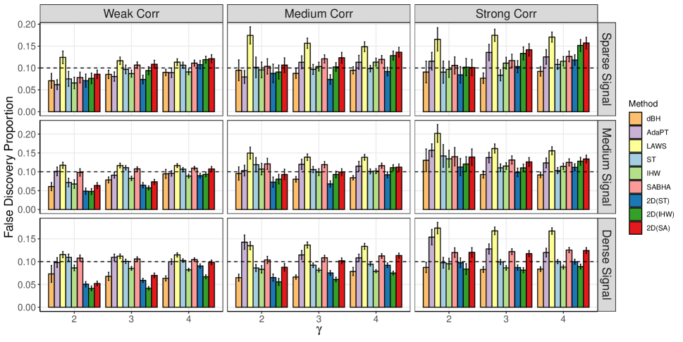
Figure 2: The mean and the standard error of FDP under Scenario I with $\gamma\in\{2,3,4\}$.

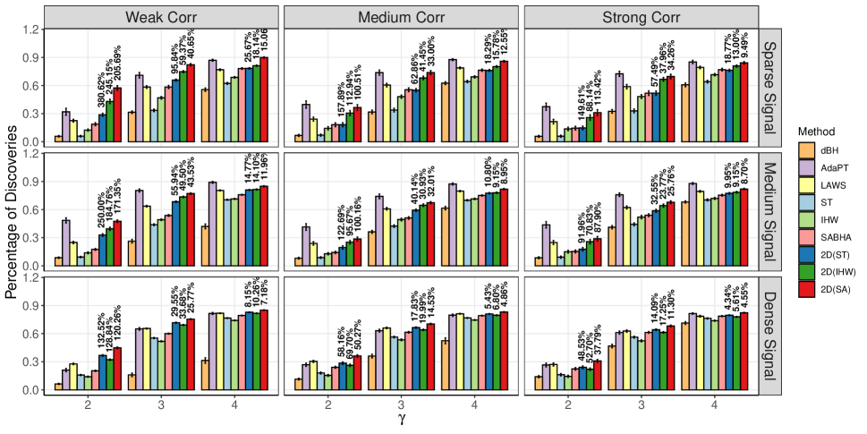
Figure 3: The mean and the standard error of power under Scenario I with $\gamma\in\{2,3,4\}$. The percentages on the top of bars represent the power improvement of 2d procedures compared to their 1d counterparts.

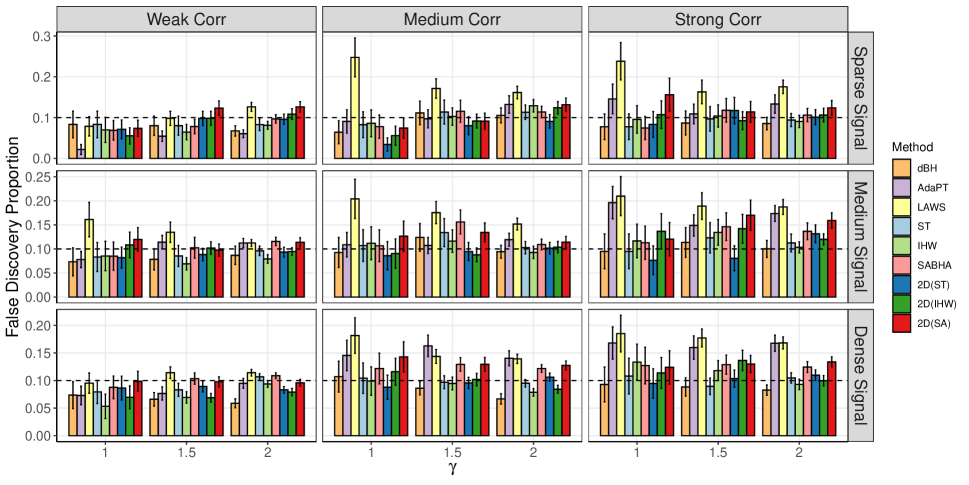
Figure 4: The mean and the standard error of FDP under Scenario II with $\gamma\in\{1,1.5,2\}$.

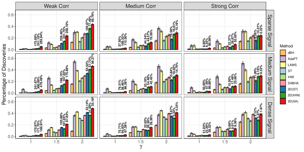
Figure 5: The mean and the standard error of power under Scenario II with $\gamma\in\{1,1.5,2\}$. The percentages on the top of bars represent the power improvement of 2d procedures compared to their 1d counterparts.

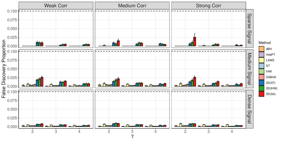
Figure 6: The mean and the standard error of FDP under Scenario III with $\gamma\in\{2,3,4\}$.

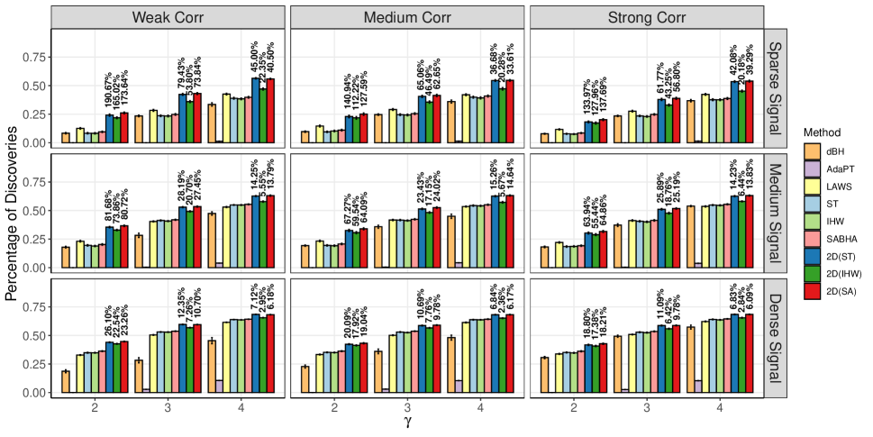
Figure 7: The mean and the standard error of power under Scenario III with $\gamma\in\{2,3,4\}$. The percentages on the top of bars represent the power improvement of 2d procedures compared to their 1d counterparts.

5.3 Two-Dimensional Domain and Unknown Covariance

In this section, we consider a spatial process $X(s)=\mu(s)+\epsilon(s)$ defined on the unit square $\mathcal{S}=[0,5]^{2}$. We observe the process on a $30\times 30$ lattice within the unit square. The noise $\epsilon(s)$ was generated from a mean-zero Gaussian process defined on $[0,5]^{2}$ with the same covariance function as described in Section 5.2 based on the distances between locations. Unlike Section 5.2, we now assume that the covariance structure is unknown, but three replications are available at each location. Given multiple realizations at each location, we could employ the maximum likelihood estimation with a pre-specified family of covariance functions to estimate the spatial covariance structure. The details are provided in Section LABEL:sec:cov_est of the Supplementary Materials. We consider two structures for the signal process $\mu(s)$.

• Scenario IV (smooth signal): $\mu_{\text{sm}}(s)=\gamma\mu_{0}(s),$ where $\mu_{0}(s)=f_{1}(s_{1})f_{2}(s_{2})$ with $s=(s_{1},s_{2})$ and $\{f_{i}\}_{i=1,2}$ being generated using B-spline functions as in Scenario I.

• Scenario V (clustered signal): $\mu_{\text{cl}}(s)=\gamma\mu_{0}(s)$, where $\mu_{0}(s)\sim\operatorname{Bernoulli}(\bar{\pi}_{0}(s))$ with

  $$\bar{\pi}_{0}(s)=\begin{cases}0.9,&\text{ if }(s_{1}-1/2)^{2}+(s_{2}-1/2)^{2}\leq(1/4)^{2},\\ 0.01,&\text{ otherwise. }\end{cases}$$

Three signal sparsity levels based on Scenarios IV and V were investigated: (1) sparse signal: $\mu_{0}(s)=\mu_{\text{cl}}(s)$; (2) medium signal: $\mu_{0}(s)=\mu_{\text{sm}}(s)$; and (3) dense signal: $\mu_{0}(s)=\mu_{\text{sm}}(s)+\mu_{\text{cl}}(s)$. The realized signal processes associated with these three sparsity levels are shown in Figure LABEL:fig:2D_Sig of the Supplementary Materials, and their corresponding percentages of the realized non-null locations are 5%, 17%, and 23%, respectively. For the magnitude $\gamma$, we set $\gamma\in\{0.5,1,1.5\}$ in both scenarios.

We report the numerical results of FDP and power of competing methods based on 50 simulation runs in Figures 8–9, respectively. Generally speaking, the 2d procedures had the best FDR and power trade-off. LAWS delivered higher power at the expense of FDR inflation. AdaPT provided reliable FDR control in all cases but their power were dominated by 2D (ST), 2D (IHW), and 2D (SA) for the sparse signal and weak correlation structures. The power improvements from the 2d procedures were most significant when the correlation was weak. It is also worth mentioning that in the case of strong correlation, the underlying covariance function was based on the Gaussian kernel while we estimated the covariance structure using the exponential kernel. The 2d procedures appeared robust to the misspecification subject to the parametric family of covariance functions.

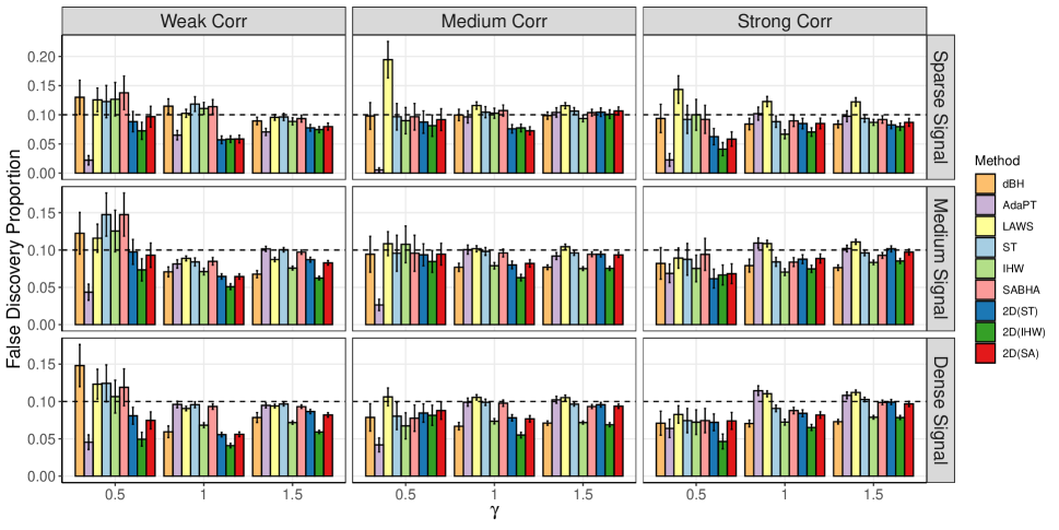
Figure 8: The mean and the standard error of FDP on the two-dimensional domain with $\gamma\in\{0.5,1,1.5\}$.

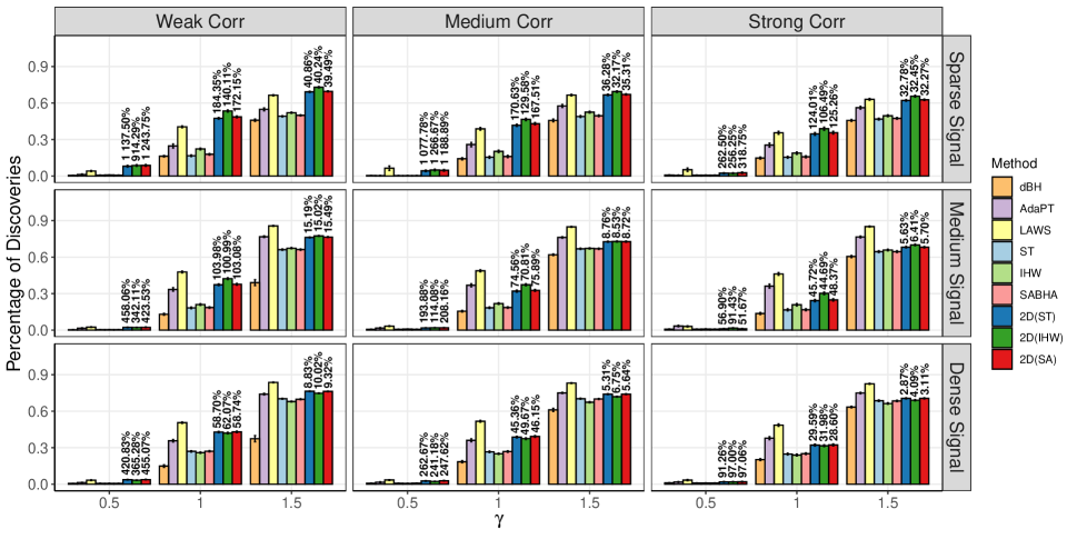
Figure 9: The mean and the standard error of power on the two-dimensional domain with $\gamma\in\{0.5,1,1.5\}$. The percentages on the top of bars represent the power improvement of 2d procedures compared to their 1d counterparts.

6 Ozone data analysis

Ozone has double-edged effects on human health: on the one hand, ozone in the upper atmosphere (stratospheric ozone) shields humans from harmful ultraviolet (UV) radiation; on the other hand, ozone at ground level (tropospheric ozone) can trigger a variety of adverse health effects on human, sensitive vegetation and ecosystems (Weinhold, 2008; Liu et al., 2022a). The US Environmental Protection Agency (EPA) formulates regulations to help states reduce tropospheric ozone levels in outdoor air. The majority of tropospheric ozone occurs through the reaction of nitrogen oxides ($\rm NO_{x}$), carbon monoxide (CO), and volatile organic compounds (VOCs) in the atmosphere when exposed to sunlight, particularly under the UV spectrum (Warneck, 2000).

We applied our proposed 2d procedures and their 1d alternatives to identify the locations where the decreasing trend is below a pre-specified level for the Contiguous United States from 2010 to 2021. The data were the annual averages of the fourth-highest daily maximum 8-hour ozone concentrations, available at the EPA’s air quality system. To facilitate the analysis, we retained 697 stations (i) having a single site, (ii) having full records across the years, and (iii) being recorded by the World Geodetic System (WGS84). We followed the procedures in Sun et al. (2015) to pre-process the data. For each location, we first fitted the linear model

$$\mathbf{X}(s)=\mu_{0}(s)+\beta(s)\mathbf{t}+\sigma_{\epsilon}(s)\bm{\epsilon}(s),$$ (16)

where $\mathbf{X}(s)=(X_{2010}(s),\cdots,X_{2021}(s))^{\top}$ was the observed ozone level measured in parts per billion (ppb), $\mathbf{t}=(2010,2011,\cdots,2021)^{\top}$ was the predictor capturing the time trend, $\beta(s)$ was the slope at site $s$, $\bm{\epsilon}(s)=(\epsilon_{2010}(s),\cdots,\epsilon_{2021}(s))^{\top}$ was assumed to follow a mean-zero Gaussian process with the exponential kernel function $k_{\epsilon}(\cdot,\cdot;r,1,\rho_{\epsilon})$, and $\sigma_{\epsilon}(s)$ was the standard deviation of noise at site $s$. We were interested in testing whether the ozone level declined more than $\beta_{0}$ ppb per year at each site, i.e., $\mathcal{H}_{0,s}:\beta(s)\geq-\beta_{0}$ versus $\mathcal{H}_{1,s}:\beta(s)<-\beta_{0}$, where $\beta_{0}\in\{0.1,0.2,0.3,0.4,0.5\}$. We first conducted simple linear regression and obtained the OLS estimates of $(\mu_{0}(s),\beta(s),\sigma_{\epsilon}(s))$, denoted as $(\widehat{\mu}_{0}(s),\widehat{\beta}(s),\widehat{\sigma}_{\epsilon}(s))$. Then, we obtained $(\widehat{r},\widehat{\rho}_{\epsilon})$ by fitting the kernel function to the residuals $\widehat{\bm{\epsilon}}(s):=\{\mathbf{X}(s)-\widehat{\beta}(s)\mathbf{t}-\widehat{\mu}_{0}(s)\}/\widehat{\sigma}_{\epsilon}(s)$. Finally, the primary test statistic was calculated as $\widehat{T}_{2}(s)=\{\widehat{\beta}(s)+\beta_{0}\}/\widehat{\sigma}_{\widehat{\beta}}(s)$, and the auxiliary test statistic was given by $\widehat{T}_{1}(s)=\sum_{v\in\mathcal{N}(s)}\{\widehat{\beta}(v)+\beta_{0}\}/\widehat{\tau}(s)$, where $\mathcal{N}(s)$ was the set containing the two-nearest neighbors of $s$ and $\widehat{\tau}(s)=\sum_{v,v^{\prime}\in\mathcal{N}(s)}\widehat{\mathrm{cov}}\{\widehat{\beta}(v),\widehat{\beta}(v^{\prime})\}$.

Locations with significant ozone level decline. We applied 2D (ST), 2D (IHW), 2D (SA), and their 1d alternatives to identify the non-null locations. We trisected the ranges of the latitude and longitude, which divided the whole area into nine different regions and allocated each site a categorical variable; see Figure LABEL:fig:ozone_reg of the Supplementary Materials for the division. Our analysis employed the categorical variable as the covariate in IHW and as the group indicator in SABHA. As shown in Figure 10, 2d procedures generally discovered more locations with significant decreasing ozone levels than their 1d counterparts did.

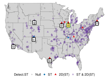
(a) $\beta_{0}=0.2$, ST versus 2D (ST)

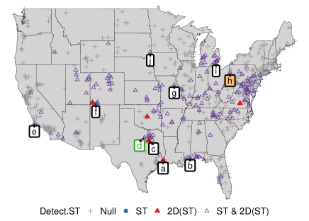
(b) $\beta_{0}=0.3$, ST versus 2D (ST)

(c) $\beta_{0}=0.3$, SABHA versus 2D (SA)

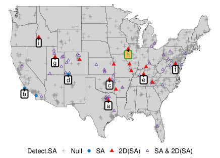
(d) $\beta_{0}=0.5$, SABHA versus 2D (SA)

Figure 10: Results for ozone data analysis. The red triangles ($\triangle$), blue circles ($\bullet$), purple triangles ($\blacktriangle$), and grey plus ($+$) signs represent the locations detected by the 2d procedure only, the 1d procedure only, both procedures, and neither one of the procedures, respectively. The labelled locations: (i) are detected by either 1d procedures or 2d procedures but not both; and (ii) possess either CO or $\rm NO_{2}$ records across 2010 to 2021. Within each sub-figure, the location with the orange background has the most significant CO decline among the labelled locations; meanwhile, the location with the green typeface has the most significant $\rm NO_{2}$ decline among the labelled locations.

Ozone precursor. The EPA has been making efforts to reduce tropospheric ozone by executing air pollution control strategies, including formulating vehicle and transportation standards, regional haze and visibility rules, and regularly reviewing the National Ambient Air Quality Standards (NAAQS). The universal ozone precursors ($\rm NO_{x}$, CO, and VOCs) first respond to these strategies and then influence the ozone levels. Indeed, some studies found the emissions of nitrogen dioxide ($\rm NO_{2}$) and CO account for the increase in background ozone levels (Chin et al., 1994; Vingarzan, 2004; Han et al., 2011). Motivated by these findings, we collected the contemporaneous CO and $\rm NO_{2}$ data from EPA and focused on the locations detected by either the 1d procedures or the 2d procedures but not both. Our goal was to scrutinize the trends of CO and $\rm NO_{2}$ at these locations and explain our findings.

To this end, we regressed the CO and $\rm NO_{2}$ levels on $\mathbf{t}$ separately and recorded the slopes to understand the increasing/decreasing trends of the CO and $\rm NO_{2}$ levels. We summarized the major findings in Figure 10 and Tables LABEL:tab:prec_descent and LABEL:tab:avr_prec (of the Supplementary Materials). First, the locations detected only by the 2d procedures always included the ones with the most significant decline in the CO or $\rm NO_{2}$ levels (i.e., the locations with the orange background or green typeface labels in Figure 10). See more details in Table LABEL:tab:prec_descent. Second, the average decline (measured by the average of the standardized slopes) of the locations detected only by the 2d procedures was larger than that of the locations detected only by the 1d procedures. Take Figure 10(d) as an example, where we had $\rm NO_{2}$ records at locations a, b, c, d, f, g, h and i, and CO records at locations b, c, e, f, and h. SABHA detected the locations b and d, while 2D (SA) identified the locations a, c, e, f, g, h and i. The average decline in the $\rm NO_{2}$ levels was -3.63 for the locations detected by SABHA as compared to -4.68 for the locations detected by 2D (SA). As for CO, the average standardized slope was -0.96 for locations detected by SABHA in comparison to -1.40 for the locations identified by 2D (SA). In general, the CO and $\rm NO_{2}$ levels tended to decrease more rapidly for those locations detected by 2D (SA) except for the case with $\beta_{0}=0.3$. See Table LABEL:tab:avr_prec for more details.

Ozone data simulation. To further validate our findings and to demonstrate the effectiveness of the 2D procedures, we conducted a simulation study where we generated data mimicking the structure of the original ozone data. In particular, we generated the ozone level data from 2010 to 2021 through (16) by setting $\beta(s)=\widehat{\beta}(s)$, $\mu(s)=\widehat{\mu}(s)$, $\sigma_{\epsilon}(s)=\widehat{\sigma}_{\epsilon}(s)$, $r=\widehat{r}$, and $\rho_{\epsilon}=\widehat{\rho}_{\epsilon}$. We processed the data and conducted multiple testing in the same way as discussed before. Table 1 shows that the 2d procedures achieved equal or slightly higher power compared to the 1d alternatives.

Table 1: Mean and standard deviation of the percentage of true discoveries in the simulated data sets mimicking the ozone data. The results are based on 50 simulation runs.

Percentage of True Discoveries
$\beta_{0}$	Methodology
	ST	IHW	SABHA	2D(ST)	2D(IHW)	2D(SA)
0.5	0.107(0.000)	0.100(0.000)	0.175(0.000)	0.107(0.000)	0.100(0.000)	0.221(0.004)
0.4	0.311(0.036)	0.302(0.040)	0.305(0.036)	0.319(0.037)	0.303(0.042)	0.322(0.038)
0.3	0.547(0.034)	0.494(0.037)	0.483(0.037)	0.556(0.033)	0.494(0.036)	0.495(0.037)
0.2	0.755(0.019)	0.660(0.021)	0.665(0.022)	0.761(0.020)	0.659(0.021)	0.674(0.022)
0.1	0.841(0.008)	0.754(0.016)	0.765(0.015)	0.845(0.009)	0.754(0.016)	0.769(0.014)

7 Discussion

This paper proposes a new FDR-controlling procedure, 2d-SMT, to improve the signal detection power by incorporating the spatial information encoded in neighboring observations. It provides a unique perspective on utilizing spatial information, which is fundamentally different from the existing covariate and structural adaptive multiple testing procedures. The spatial information is gathered through an auxiliary statistic, which is used to screen out the noise. A primary statistic from the location of interest is then used to determine the existence of the signal. 2d-SMT is particularly effective when the signals exhibit in clusters. We establish the asymptotic FDR control for 2d-SMT under weak spatial dependence and demonstrate its usefulness through simulation studies and the analysis of an ozone data set.

To conclude, we point out a few future research directions. First, as discussed in Section 2.7, the proposed 2d-SMT is flexible to combine with various weighted BH procedures. One challenge is, however, to establish a rigorous theoretical FDR control guarantee for the resulting weighted 2d-SMT procedures. Second, when implementing our methodology, we use the $\kappa$-nearest neighbors to construct the auxiliary statistic. A more delicate strategy is to apply a weighting scheme to pool sufficient information from nearby locations. Third, extending the idea in 2d-SMT to other statistical problems, such as mediation analysis in causal inference, is of interest.

References

- Basu et al. (2018) Basu, P., Cai, T. T., Das, K., and Sun, W. (2018), “Weighted false discovery rate control in large-scale multiple testing,” Journal of the American Statistical Association, 113, 1172–1183.
- Benjamini and Heller (2007) Benjamini, Y. and Heller, R. (2007), “False discovery rates for spatial signals,” Journal of the American Statistical Association, 102, 1272–1281.
- Benjamini and Hochberg (1995) Benjamini, Y. and Hochberg, Y. (1995), “Controlling the false discovery rate: A practical and powerful approach to multiple testing,” Journal of the Royal Statistical Society: Series B (Methodological), 57, 289–300.
- Cai et al. (2021) Cai, T. T., Sun, W., and Xia, Y. (2021), “LAWS: A locally adaptive weighting and screening approach to spatial multiple testing,” Journal of the American Statistical Association, 0, 1–14.
- Cao et al. (2022) Cao, H., Chen, J., and Zhang, X. (2022), “Optimal false discovery rate control for large scale multiple testing with auxiliary information,” The Annals of Statistics, 50, 807–857.
- Chin et al. (1994) Chin, M., Jacob, D. J., Munger, J. W., Parrish, D. D., and Doddridge, B. G. (1994), “Relationship of ozone and carbon monoxide over North America,” Journal of Geophysical Research: Atmospheres, 99, 14565–14573.
- Fithian and Lei (2020) Fithian, W. and Lei, L. (2020), “Conditional calibration for false discovery rate control under dependence,” arXiv preprint, abs/2201.1004.
- Genovese et al. (2006) Genovese, C. R., Roeder, K., and Wasserman, L. (2006), “False discovery control with p-value weighting,” Biometrika, 93, 509–524.
- Han et al. (2011) Han, S., Bian, H., Feng, Y., Liu, A., Li, X., Zeng, F., Zhang, X., et al. (2011), “Analysis of the relationship between O3, NO and NO2 in Tianjin, China,” Aerosol and Air Quality Research, 11, 128–139.
- Heller et al. (2006) Heller, R., Stanley, D., Yekutieli, D., Rubin, N., and Benjamini, Y. J. N. (2006), “Cluster-based analysis of FMRI data,” Neuroimage, 33, 599–608.
- Hu et al. (2010) Hu, J., Zhao, H., and Zhou, H. (2010), “False discovery rate control with groups,” Journal of the American Statistical Association, 105, 1215–1227.
- Huang et al. (2021) Huang, H.-C., Cressie, N., Zammit-Mangion, A., and Huang, G. (2021), “False discovery rates to detect signals from incomplete spatially aggregated data,” Journal of Computational and Graphical Statistics, 30, 1081–1094.
- Ignatiadis and Huber (2021) Ignatiadis, N. and Huber, W. (2021), “Covariate powered cross-weighted multiple testing,” Journal of the Royal Statistical Society: Series B (Statistical Methodology), 83, 720–751.
- Ignatiadis et al. (2016) Ignatiadis, N., Klaus, B., Zaugg, J. B., and Huber, W. (2016), “Data-driven hypothesis weighting increases detection power in genome-scale multiple testing,” Nature Methods, 13, 577–580.
- Jenish (2012) Jenish, N. (2012), “Nonparametric spatial regression under near-epoch dependence,” Journal of Econometrics, 167, 224–239.
- Jenish and Prucha (2012) Jenish, N. and Prucha, I. R. (2012), “On spatial processes and asymptotic inference under near-epoch dependence,” Journal of Econometrics, 170, 178–190.
- Jiang and Zhang (2009) Jiang, W. and Zhang, C.-H. (2009), “General maximum likelihood empirical Bayes estimation of normal means,” The Annals of Statistics, 37, 1647–1684.
- Katzfuss and Guinness (2021) Katzfuss, M. and Guinness, J. (2021), “A general framework for Vecchia approximations of Gaussian processes,” Statistical Science, 36, 124–141.
- Kiefer and Wolfowitz (1956) Kiefer, J. and Wolfowitz, J. (1956), “Consistency of the maximum likelihood estimator in the presence of infinitely many incidental parameters,” The Annals of Mathematical Statistics, 27, 887–906.
- Koenker and Gu (2017) Koenker, R. and Gu, J. (2017), “REBayes: An R package for empirical Bayes mixture methods,” Journal of Statistical Software, 82, 1–26.
- Koenker and Mizera (2014) Koenker, R. and Mizera, I. (2014), “Convex optimization, shape constraints, compound decisions, and empirical Bayes rules,” Journal of the American Statistical Association, 109, 674–685.
- Lei et al. (2018) Lei, J., G’Sell, M., Rinaldo, A., Tibshirani, R. J., and Wasserman, L. (2018), “Distribution-free predictive inference for regression,” Journal of the American Statistical Association, 113, 1094–1111.
- Li and Barber (2019) Li, A. and Barber, R. F. (2019), “Multiple testing with the structure-adaptive Benjamini-Hochberg algorithm,” Journal of the Royal Statistical Society: Series B (Statistical Methodology), 81, 45–74.
- Liu et al. (2022a) Liu, W., Hegglin, M. I., Checa-Garcia, R., Li, S., Gillett, N. P., Lyu, K., Zhang, X., and Swart, N. C. (2022a), “Stratospheric ozone depletion and tropospheric ozone increases drive Southern Ocean interior warming,” Nature Climate Change, 12, 365–372.
- Liu et al. (2022b) Liu, W., Ke, Y., Liu, J., and Li, R. (2022b), “Model-Free Feature Screening and FDR Control With Knockoff Features,” Journal of the American Statistical Association, 117, 428–443.
- Mardia and Marshall (1984) Mardia, K. V. and Marshall, R. J. (1984), “Maximum likelihood estimation of models for residual covariance in spatial regression,” Biometrika, 71, 135–146.
- Padoan and Bevilacqua (2015) Padoan, S. A. and Bevilacqua, M. (2015), “Analysis of random fields using CompRandFld,” Journal of Statistical Software, 63, 1–27.
- Sang and Huang (2012) Sang, H. and Huang, J. Z. (2012), “A full scale approximation of covariance functions for large spatial data sets,” Journal of the Royal Statistical Society: Series B (Statistical Methodology), 74, 111–132.
- Scott et al. (2015) Scott, J. G., Kelly, R. C., Smith, M. A., Zhou, P., and Kass, R. E. (2015), “False discovery rate regression: An application to neural synchrony detection in primary visual cortex,” Journal of the American Statistical Association, 110, 459–471.
- Shen et al. (2002) Shen, X., Huang, H.-C., and Cressie, N. (2002), “Nonparametric hypothesis testing for a spatial signal,” Journal of the American Statistical Association, 97, 1122–1140.
- Sommerfeld et al. (2018) Sommerfeld, M., Sain, S., and Schwartzman, A. (2018), “Confidence regions for spatial excursion sets from repeated random field observations, with an application to climate,” Journal of the American Statistical Association, 113, 1327–1340.
- Storey (2002) Storey, J. D. (2002), “A direct approach to false discovery rates,” Journal of the Royal Statistical Society: Series B (Methodological), 64, 479–498.
- Storey et al. (2004) Storey, J. D., Taylor, J. E., and Siegmund, D. (2004), “Strong control, conservative point estimation and simultaneous conservative consistency of false discovery rates: a unified approach,” Journal of the Royal Statistical Society: Series B (Statistical Methodology), 66, 187–205.
- Sun et al. (2015) Sun, W., Reich, B. J., Cai, T. T., Guindani, M., and Schwartzman, A. (2015), “False discovery control in large-scale spatial multiple testing,” Journal of the Royal Statistical Society: Series B (Statistical Methodology), 77, 59–83.
- Tansey et al. (2018) Tansey, W., Koyejo, O., Poldrack, R. A., and Scott, J. G. (2018), “False discovery rate smoothing,” Journal of the American Statistical Association, 113, 1156–1171.
- Vingarzan (2004) Vingarzan, R. (2004), “A review of surface ozone background levels and trends,” Atmospheric Environment, 38, 3431–3442.
- Warneck (2000) Warneck, P. (2000), “Chapter 5 Ozone in the troposphere,” in Chemistry of the Natural Atmosphere, ed. Warneck, P., Academic Press, vol. 71 of International Geophysics, pp. 211–263.
- Wasserman and Roeder (2009) Wasserman, L. and Roeder, K. (2009), “High dimensional variable selection,” Annals of statistics, 37, 2178–2201.
- Weinhold (2008) Weinhold, B. (2008), “Ozone nation: EPA standard panned by the people,” Environmental Health Perspectives, 116, A302–A305.
- Yi et al. (2021) Yi, S., Zhang, X., Yang, L., Huang, J., Liu, Y., Wang, C., Schaid, D. J., and Chen, J. (2021), “2dFDR: A new approach to confounder adjustment substantially increases detection power in omics association studies,” Genome Biology, 22, 208.
- Yun et al. (2022) Yun, S., Zhang, X., and Li, B. (2022), “Detection of local differences in spatial characteristics between two spatiotemporal random fields,” Journal of the American Statistical Association, 117, 291–306.
- Zhang and Chen (2022) Zhang, X. and Chen, J. (2022), “Covariate adaptive false discovery rate control with applications to omics-wide multiple testing,” Journal of the American Statistical Association, 117, 411–427.